Trends in distributional characteristics: Existence of ...jgonzalo/TrendDistributional... · Trends in distributional characteristics: Existence of global warming Mar a Dolores Gadea

Trends in distributional characteristics:

Existence of global warming ∗

Marıa Dolores Gadea Rivas †

University of Zaragoza

Jesus Gonzalo ‡

U. Carlos III de Madrid

March 2018

Abstract

What type of global warming exists? This study introduces a novel methodol-ogy to answer this question, which is the starting point for all issues related toclimate change analyses. Global warming is defined as an increasing trend incertain distributional characteristics (moments, quantiles, etc.) of global tem-peratures, in addition to simply examining the average values. Temperaturesare viewed as a functional stochastic process from which we obtain distribu-tional characteristics as time series objects. Here, we present a simple robusttrend test and prove that it is able to detect the existence of an unknown trendcomponent (deterministic or stochastic) in these characteristics. Applying thistrend test to daily temperatures in Central England (for the period 1772–2017)and to global cross-sectional temperatures (1880–2015), we obtain the samestrong conclusions: (i) there is an increasing trend in all distributional charac-teristics (time series and cross-sectional), and this trend is larger in the lowerquantiles than it is in the mean, median, and upper quantiles; (ii) there is anegative trend in the characteristics that measure dispersion (i.e., lower tem-peratures approach the median faster than higher temperatures do). This typeof global warming has more serious consequences than those found by analyzingonly the average.

JEL classification: C31, C32, Q54Keywords: Climate change; Global–Local warming; Functional stochastic pro-cess; Distributional characteristic; Trend; Quantile; Temperature distribution

∗We are grateful to an editor, three anonymous referees and conference and seminar participants at

Econometric Models of Climate Change (Aarhus), 11th World Congress of the Econometric Society (Mon-

treal), IAAE (London), Time Series Econometrics Workshop (Zaragoza), CFE-ERCIM (Oviedo), EUI

(Firenze), ESSEC (Paris), U. of Loughborough, U. of Notthingham, Nuffield College and INET (Oxford),

Erasmus School of Economics (Rotterdam), U. of Manchester, U. of Lancaster, Durham University and

SUFE (Shanghai) for insightful comments and suggestions. Special thanks to David Lister (U. East Anglia

and CRU) for his assistance with the HadCRUT4 global temperature database. Financial support from

the Spanish MINECO (grants ECO2016-78652, ECO2017-83255-C3-1-P and ECO2017-83255-C3-3-P and

Maria de Maeztu grant MDM 2014-0431), Bank of Spain (ER grant program), and MadEco-CM (grant

S2015/HUM-3444) is also gratefully acknowledged.† Department of Applied Economics, University of Zaragoza. Gran Vıa, 4, 50005 Zaragoza (Spain). Tel:

+34 9767 61842, fax: +34 976 761840 and e-mail: [email protected]‡ Department of Economics, University Carlos III, Madrid 126 28903 Getafe (Spain). Tel: +34 91

6249853, fax: +34 91 6249329 and e-mail: [email protected]

1

Trends in distributional characteristics. 2

1 Introduction

According to the Intergovernmental Panel on Climate Change (IPCC), the study of

climate change, and particularly global warming (GW), involves a careful analysis

of the following four issues or questions, which form a chain (see IPCC, 2014): (i)

What type of GW exists?; (ii) causes of GW (is GW caused by human activities?);

(iii) economic effects of GW; and (iv) economic policies to mitigate these effects.

Obviously, to determine the type of GW is crucial for the next issues in the chain.

The purpose of this paper is to offer a complete answer to the first question by

analyzing the characteristics of the existent GW. We investigate these characteristics

by introducing a novel methodology to analyze trends. This methodology is also

valid for quantitative analyses of many other important economic issues that require

a thorough study of trend behaviors (e.g., trends in GDP, debt, inequality, etc.).

We start by defining GW as an increasing trend in global temperatures. In

this study, a trend is understood in a broader sense than is currently accepted in

the literature (see White and Granger, 2011). As such, we look for trends in the

characteristics (moments, quantiles, etc.) of the temperature distribution, and do

not simply focus on average values. For instance, a random walk has a trend in the

variance, but not in the mean. Furthermore, the average temperature might not

show any growth pattern, but the lower tail might show a clear increase. According

to the standard definition in the literature, this would not be interpreted as GW,

but using the proposed methodology, it clearly would. Even when the average

shows some growth, having a wider view of the “trending” behavior of the whole

distribution will help in the analysis of the remaining three questions in the chain.

There is an extensive body of literature that analyzes the trend behavior (de-

terministic and stochastic) of the mean of the temperature distribution (see Harvey

and Mills, 2003; Hendry and Pretis, 2013; Gay-Garcıa et al., 2009; Mills, 2010;

Kauffmann et al., 2006, 2010, 2013; Estrada et al., 2013; Chang et al., 2015, etc.)

This approach corresponds to the standard popular definition of climate: climate is

the average of weather. In contrast, our proposed method for analyzing trends in

the distributional characteristics agrees more with the definition adopted by clima-

tologists: climate is the statistics of weather. This definition (see the IPCC 2014

glossary of definitions) includes not just the average, but also statistics on variability,

tail behavior, and so on.

For the purpose of this research, global temperatures are treated as a functional


stochastic process, X = (Xt(ω), t ∈ T ), where T is an interval in R, defined on a

probability space (Ω,=, P ), such that t→ Xt(ω) belongs to some function space G,

for all ω ∈ Ω. Here, X defines a G-valued stochastic process. Note that G can be a

Hilbert space, as in Bosq (2000) (AR-H model for sequences of random Hilbert func-

tions X1(ω), X2(ω), ..., XT (ω)), Park and Qian (2012), and Chang et al. (2015, 2016)

(regression models for sequences of random state densities f1(ω), f2(ω), ..., fT (ω)).

Alternatively, it can be a Banach space for sequences of random state distributions

(F1(ω), F2(ω), ..., FT (ω)). Instead of modeling the whole sequence of G functions,

as previous authors do, we present an alternative approach where we model certain

characteristics, Ct, of these functions: the state mean, the state variance, the state

quantiles, and so on. The main advantage of this approach, apart from its simplic-

ity, is that these characteristics become time series objects. Therefore, we can apply

existing tools used in the time series literature for modeling, inference, forecasting,

and so on. This alternative proposal resembles the quantile curve estimation ap-

proach of Draghicescu et al. (2009), as well as the realized volatility modeling of

high-frequency data in financial econometrics (see Andersen et al., 2003, 2006).

We assume that at each period t, we have N observations from higher-frequency

time series or from cross-sectional units. From these observations, we obtain relevant

characteristics, which we convert into time series objects. In order to detect trend

behavior in these characteristics, we test β = 0 in the following simple least squares

(LS) regression: Ct = α+βt+ut. This regression needs to be understood as the best

linear LS approximation to an unknown trend function (see White, 1980). We prove

that the t-test (β = 0) is able to detect the standard deterministic trends used in the

literature (see Davis, 1941), as well as stochastic trends generated by long-memory,

near-unit-root, and local-level models (see Mueller and Watson, 2008).

In order to show the generality of our results, we implement two applications: one

with N time series observations for each year t, and another with N cross-sectional

observations, also for each year t. The first application studies the trend behavior of

the distributional characteristics of temperature in Central England from January 1,

1772, to October 31, 2017. To ensure the robustness of our findings, we also present

results for temperatures in other locations (Stockholm, Cadiz, and Milan). In the

second application, we analyze global temperatures across different stations in the

Northern and Southern Hemispheres for the period 1880–2015. The two applications

lead to similar trend results, which can be summarized as follows. First, there exists

a trend in most of the characteristics considered. The trend in the lower quantiles is


stronger than those in the mean and upper quantiles of the temperature distribution

(the IPCC 2014 reports a decrease in cold temperature extremes and an increase in

warm temperature extremes). Second, dispersion measures such as the interquartile

range (iqr), standard deviation (std), and range (max − min) show a negative

trend (a possible cause for this fact is suggested in Arrhenius, 1896). Therefore,

we conclude that GW is not only a phenomenon of an increase in the average

temperature, but also of a larger increase in lower temperatures, leading to decreased

dispersion. Ignoring these facts could have serious consequences for climate analyses

(e.g., an acceleration in global ice melting) and, therefore, they should be considered

in all future international climate agreements. Present agreements focus only on the

mean characteristic.

The rest of the paper is organized as follows. In Section 2, we define GW and the

trends we use to investigate GW. In Section 3, we present our basic framework for the

time series analysis. In Section 4, we introduce and analyze our proposed trend test

(TT ) to detect a general unknown trend behavior in any distributional characteristic.

Section 5 provides two empirical applications: using a purely temporal dimension

(local daily temperature on an annual basis), and using a cross-sectional dimension

(global temperatures measured annually, by station). Finally, Section 6 concludes

the paper. The Appendix contains detailed proofs of the main results, as well as

the finite-sample performance of our proposed test and additional empirical results.

2 Global Warming and Trends

In this section, we introduce our definition of GW, as well as the definition of trend

that we use to characterize the type of existent GW.

Definition 1. (Global warming): Global warming is defined as the existence of anincreasing trend in some of the characteristics measuring the central tendency orposition (quantiles) of the global temperature distribution.

Under this definition, the existence of a trend in other types of characteris-

tics like, for instance, those measuring dispersion or symmetry will not constitute

warming but clearly can help to describe it. As mentioned in the Introduction,

this definition agrees with the climatologist definition of climate: the statistics of

weather. As such, it includes not just the average temperature, but also its distribu-

tional behavior. The key issue is to find a useful definition and characterization of a

trend. Surprisingly, not many statistical or econometric books dedicate a chapter to


this topic. As noted by Phillips (2005), this may be because “[n]o one understands

trends, but everyone sees them in the data.” Exceptions to this include books by

Davis (1941), Anderson (1971), and Kendall and Stuart (1983). However, even these

do not provide a definition or characterization of a trend that would be useful for our

GW analysis. Instead, a useful definition is provided in White and Granger (2011)

(WG): (i) a trend should have a direction; (ii) a trend should be basically smooth;

(iii) a trend does not have to be monotonic throughout; and (iv) a trend can be

a local behavior (observed trends can be related to a particular section of data).

These characterizations are formalized by WG in the following two definitions, one

for deterministic trends and the other for stochastic trends.

Definition 2. (Deterministic trend (WG, 2011)): Let Ct = Ct : t = 0, 1, ... bea sequence of real numbers. If Ct < Ct+1 for all t, then Ct is a strictly increasingtrend. If Ct ≤ Ct+1 for all t and there exists a countable subsequence Ctj suchthat Ctj is a strictly increasing trend, then Ct is an increasing trend. If −Ctis a strictly increasing (an increasing) trend, then Ct is a strictly decreasing (adecreasing) trend.

If definition 2 is only satisfied for all t1 ≤ t < t2 then Ct is a strictly increasing

(or an increasing) local trend in [t1, t2].

Example of a deterministic trend: A polynomial trend for certain values of the

β parameters Ct = β0 + β1t+ β2t2 + ...+ βkt

k.

Additional examples can be found in Chapters 1 and 6 of Davis (1941) and in

WG.

Definition 3. Stochastic trend (WG, 2011)): Let Xt be a stochastic process.

• Consider Ct = E(Xt). If Ct is a strictly increasing (an increasing) trend, thenXt has a strictly increasing (an increasing) trend in the mean.

• Let Ct = E(|Xt − E(Xt)|k), for finite positive real k. If Ct is a strictly increas-ing (an increasing) trend, then Xt has a strictly increasing (an increasing)trend in the kth absolute central moment.

• Let Ct(p) = infxεR : Ft(x) ≥ p be the quantile p ∈ (0, 1) of the distributionfunction Ft(x) = P (Xt ≤ x). If Ct(p) is strictly increasing (an increasing)trend, then Xt has a strictly increasing (an increasing) trend in quantile p.

Examples of stochastic trends:

- A random walk Xt = Xt−1 + ut has a trend in the variance, but not in themean.


- A random walk with drift Xt = α+Xt−1 + ut has a trend in the mean and inthe variance.

More examples can be found in Mueller and Watson (2008).

Note that, from Definition 3, the concept of a stochastic trend considered in

the econometrics literature now becomes a pure deterministic trend in the second

moment of the distribution. This implies that by developing a method able to

detect deterministic trends, and applying this method to different distributional

characteristics, we can detect any type of trend. This method is introduced in

Section 4. First, in the next section, we present the basic framework for our proposed

time series analysis, which we use to obtain the distributional characteristics as time

series objects.

3 Basic Framework for a Time Series Analysis

In this study, temperature is viewed as a functional stochastic process, X = (Xt(ω), t ∈T ), where T is an interval in R, defined on a probability space (Ω,=, P ), such that

t → Xt(ω) belongs to some function space G, for all ω ∈ Ω. Here, X defines a

G-valued stochastic process.

This function space G is equipped with a scalar product < ., . > and/or a norm

‖ . ‖, and a Borel σ-algebra, BG. It is separable and complete. Thus, G can be a

Hilbert space, as in Bosq (2000) (AR-H model for sequences of random Hilbert func-

tions X1(ω), X2(ω), ..., XT (ω)), Park and Qian (2012), and Chang et al. (2015, 2016)

(regression models for sequences of random state densities f1(ω), f2(ω), ..., fT (ω)), a

Banach space for a sequence of random state distributions (F1(ω), F2(ω), ..., FT (ω)),

etc.

A convenient example of an infinite-dimensional discrete-time process is that of

associating a sequence of random variables with values in an appropriated function

space, where ξ = (ξn, n ∈ R+). This may be obtained by setting

Xt(n) = ξtN+n, 0 ≤ n ≤ N, t = 0, 1, 2, ..., T. (1)

Thus, X = (Xt, t = 0, 1, 2, ..., T ). If the sample paths of ξ are continuous, then we

have a sequence X0, X1, .... of random variables in the space C[0, N ]. The choice

of the period or segment t is compelling in many specific situations. In our case, t

denotes the year, and N can represent temporal or cross-sectional observations.


We may wish to model the whole sequence of G functions, for instance, the

sequence of state densities (f1(ω), f2(ω), ..., fT (ω)), as in Chang et al. (2015, 2016).

Alternatively, we may wish to model only certain characteristics (Ct(w)) of these

G functions, for instance, the state mean, state variance, state quantile, and so on.

These characteristics can be considered as time series objects, which means we can

apply existing econometrics tools to Ct(w). For this reason, we follow the second

option, which resembles the quantile curve estimation analyzed in Draghicescu et al.

(2009) and in Zhou and Wu (2009). In terms of the variance characteristic, it also

resembles the literature on realized volatility (Andersen et al., 2003, 2006). Using

this characteristic approach, we move from Ω to RT , as in a standard stochastic

process, passing through a G functional space:

Ω(w)

X−→ GXt(w)

C−→ RCt(w)

.

Returning to the convenient example and abusing the notation, the stochastic

structure can be summarized in the following array:

X10(w) = ξ0(w) X11(w) = ξ1(w) . . . X1N (w) = ξN (w) C1(w)

X20(w) = ξN+1(w) X21(w) = ξN+2(w) . . . X2N (w) = ξ2N (w) C2(w)

.

.

.

.

.

.

. . .

. . .

. . .

.

.

.

.

.

.

XT0(w) = ξ(T−1)N+1(w) XT1(w) = ξ(T−1)N+2(w) . . . XTN (w) = ξTN (w) CT (w).

(2)

Throughout this paper, similarly to the assumptions made in Park and Qian

(2012) and Chang et al. (2016), we assume that in each period, t, there are sufficient

temporal or cross-sectional observations (N → ∞) for these characteristics to be

estimated consistently.

Assumption 3.1. In each period, t, the stochastic functional processX = (Xt(ω), t ∈T ) satisfies certain regularity conditions, such that the state densities, distributionand, therefore, quantiles are estimated consistently.

In the temporal framework, local stationarity (Dahlhaus, 2009) plus some strong

mixing conditions (Hansen, 2008) are sufficient to obtain uniform ““strong”” consis-

tency for suitable regular kernel estimators of the state densities. Local stationarity

plus some ϕ-mixing conditions (see Degenhardt et al. 1996) are sufficient for the

central limit theorem to hold for smoothed empirical distribution functions and for


smoothed sample quantiles for each period or segment, t. For the cross-sectional situ-

ation, similar results hold (e.g., Silverman, 1978) if the state distributions are defined

as cross-sectional distributions, and if independent and identically distributed ob-

servations are available to estimate them for each period (for dependency among N

observations, see Bosq (1998, Thm 2.2) and for clustered data, see Breunig (2001)).

4 Testing for a Trend

The objective of this section is to provide a simple test to detect the existence of a

general unknown trend component in a given characteristic Ct of Xt. To do this,

we need to convert Definition 3 into a more practical definition.

Definition 4. (Practical definition 1): Let h(t) be an increasing function of t. Acharacteristic Ct of a functional stochastic process Xt contains a trend if β 6= 0 inthe regression

Ct = α+ βh(t) + ut, t = 1, ..., T. (3)

This definition has its natural local trend version. From this definition, two

questions arise that need to be answered. First, we need to specify which func-

tion h(t) to use in regression (3), and second, we have to design a proper test for

the null hypothesis of interest, β = 0. Before resolving these two questions, the

practical Definition 4 requires some preliminary concepts and results, in particular,

the concept of summability (see Berenguer-Rico and Gonzalo 2014, for a stochastic

version).

Definition 5. (Order of Summability): A trend h(t) is said to be summable oforder “δ” (S(δ)) if there exists a slowly varying function L(T ),1 such that

ST =1

T 1+δL(T )

T∑t=1

h(t) (5)

is O(1), but not o(1).

The following examples illustrate the order of summability:

1A positive Lebesgue measurable function, L, on (0,∞) is slowly varying (in Karamata’s sense)at ∞ if

L(λn)

L(n)→ 1 (n→∞) ∀λ > 0. (4)

(See Embrechts et al., 1999, p. 564).


Example 4.1. Let h(t) = c( 6= 0). Then, 1T

∑Tt=1 c = c. Therefore, δ = 0.

Example 4.2. Let h(t) = tk. Then, 1T 1+k

∑Tt=1 t

k = O(1). Therefore, δ = k.

Example 4.3. Let h(t) = e λt. Then, 1eλT

∑Tt=1 e

λt = O(1). Therefore, δT =λT

Log(T ) − 1→∞, as T →∞.

Example 4.4. Let h(t) = K1+Be−λt

. Then, 1T

∑Tt=1

K1+Be−λt

= O(1). Therefore,δ = 0.

Example 4.5. Let h(t) = Log(t). Then, 1TLog(T )

∑Tt=1 Log(t) = O(1). Therefore,

δ = 0.

Example 4.6. Let h(t) = 1t . Then, 1

Log(T )

∑Tt=1

1t = O(1). Therefore, δ = −1.

The properties of the OLS estimator β in regression (3) depend on the balance

between the trend components of the dependent variable Ct and the regressor h(t).

To characterize this balance, we need the following definition.

Definition 6. (Trend strength): A trend function h(t) is said to be stronger thananother trend function g(t) if δh > δg.

Now, using Definitions 5 and 6, we have all the necessary elements to present

our trend test to detect a general trend component in a given characteristic Ct =

h(t) + I(0),2 with h(t) unknown. First, we recall a well-known related result (see

Hamilton, 1994, Chapter 16):

Proposition 1. Let Ct = I(0). In the LS regression

Ct = α+ βt+ ut, (6)

the OLS estimator satisfiesT 3/2β = Op(1) (7)

and asymptotically (T →∞)tβ=0 is N(0, 1).

Proposition 2. Let Ct = h(t) + I(0), such that h(t) is an increasing S(δ) functionwith δ ≥ 0, and the function g(t) = h(t)t is S(δ + 1). In the LS regression

Ct = α+ βt+ ut, (8)

2Our definition of an I(0) process follows Johansen (1995). A stochastic process Yt that satisfies

Yt−E(Yt) =∞∑i=1

Ψiεt−i is called I(0) if∞∑i=1

Ψ izi converges for |z| < 1 + δ, for some δ > 0 and

∞∑i=1

Ψ

i 6= 0, where the condition εt ∼ iid(0,σ2) with σ2 > 0 is understood.


the OLS β estimator satisfies

T (1−δ)β = Op(1). (9)

In order to analyze the behavior of the t-statistic tβ = 0, we assume that thefunction h(t)2 is S(1 + 2δ− γ), with 0 ≤ γ ≤ 1 + δ. Then, the t-statistic diverges atthe following rates

tβ=0 =

Op(T

γ/2) for 0 ≤ γ ≤ 1

Op(T1/2) for 1 ≤ γ ≤ 1 + δ.

(10)

Proof in Appendix A.

The following examples illustrate how to use Proposition 2:

Example 4.7. Let Ct = h(t) + I(0), with h(t) = t2. The summability parametersare δ = 2 and γ = 1. Then, in regression (8), β and tβ=0 diverges as T→∞.

Example 4.8. Let Ct = h(t) + I(0), with h(t) = t. The summability parametersare δ = 1 and γ = 1. Then, in regression (8), β = Op(1); but, tβ=0 diverges asT→∞.

Example 4.9. Let Ct = h(t) + I(0), with h(t) = t1/2. The summability parameters

are δ = 1/2 and γ = 1. Then, in regression (8), βp→ 0; but, tβ=0 diverges as T→∞.

Example 4.10. Let Ct = h(t) + I(0), with h(t) = log(t). The summability param-

eters are δ = 0 and γ = 1. Then, in regression (8), βp→ 0; but, tβ=0 diverges as

T→∞.

Example 4.11. Let Ct = h(t)+I(0), with h(t) = e λt . The summability parametersare δT = λT

Log(T ) −1 and γ = 0. Then, in regression (8), β diverges and tβ=0 = Op(1)

as T→∞. It can be proved that, asymptotically, tβ=0 > z0.95 for λ ∈ (0, 2.095).

Example 4.12. Let Ct = h(t) + I(0), with h(t) = K1+Be−λt

. The summability

parameters are δ = 0 and γ = 1. Then, in regression (8), βp→ 0; but, tβ=0 diverges

as T→∞.

A question of great empirical importance is how does our trend test of Propo-

sition 2 behave when Ct = I(1). Following Durlauf and Phillips (1988), T 1/2β =

Op(1); however, tβ=0 diverges as T→∞. Therefore, our trend test can detect the

stochastic trend generated by an I(1) process. In fact, our test will detect trends

generated by any of the three standard persistent processes considered in the lit-

erature (see Muller and Watson, 2008): (i) fractional or long-memory models; (ii)

near-unit-root AR models; and (iii) local-level models. Let


Ct = µ+ zt, t = 1, ..., T. (11)

In the first model, zt is a fractional process with 1/2 < d < 3/2. In the second

model, zt follows an AR, with its largest root close to unity, ρT = 1 − c/T . In the

third model, zt is decomposed into an I(1) and an I(0) component. Its simplest

format is zt = υt + εt with υt = υt−1 +ηt, where εt is ID(0, q ∗ σ2), ηt is ID(0, σ2),

σ2 > 0 and both disturbances are serially and mutually independent. Note that the

pure unit-root process is nested in all three models: d = 1, c = 0, and q = 0.

The long-run properties implied by each of these models can be characterized

using the stochastic properties of the partial sum process for zt. The standard

assumptions considered in the macroeconomics or finance literature assume the ex-

istence of a “δ,” such that T−1/2+δ∑T

t=1 zt −→ σ H(.), where “δ” is a model-specific

constant and H is a model-specific zero-mean Gaussian process with a given covari-

ance kernel k(r, s). Then, it is clear that the process Ct = µ + zt is summable (see

Berenguer-Rico and Gonzalo, 2014). This is the main reason why Proposition 3

holds for these three persistent processes.

Proposition 3. Let Ct = µ + zt, t = 1, ..., T , with zt any of the following threeprocesses: (i) a fractional or long-memory model, with 1/2 < d < 3/2; (ii) a near-unit-root AR model; or (iii) a local-level model. Furthermore, T−1/2+δ

∑Tt=1 zt −→ σ

H(.), where “δ” is a model-specific constant and H is a model-specific zero-meanGaussian process with a given covariance kernel k(r, s). Then, in the LS regression

Ct = α+ βt+ ut,

the t-statistic diverges,tβ=0 = Op(T

1/2).

Proof in Appendix A.

In summary, Propositions 2 and 3 imply that Definition 4 can be simplified to

the following practical definition.

Definition 7. (Practical definition 2): A characteristic Ct of a functional stochasticprocess Xt contains a trend if in the LS regression,

Ct = α+ βt+ ut, t = 1, ..., T, (12)

β = 0 is rejected.

Several remarks are relevant with respect to this definition: (i) regression (12)

has to be understood as the linear LS approximation of an unknown trend function


h(t) (see White, 1980); (ii) the parameter β is the plim of βols; (iii) if the regression

(12) is the true data-generating process, with ut ∼ I(0), then the OLS β estimator

is asymptotically equivalent to the GLS estimator (see Grenander and Rosenblatt,

1957); and (iv) in practice, in order to test β = 0, it is recommended to use a robust

HAC version of tβ=0 (see Busetti and Harvey, 2008).

For all these reasons, in the empirical applications we implement Definition 7

by estimating regression (12) using OLS and constructing a HAC version of tβ=0

(Newey and West, 1987). Appendix B includes a detailed analysis of the finite-

sample performance of this test for several types of the most common deterministic

and stochastic trends. Alternative estimation and testing procedures for certain

types of polynomial deterministic trends can be found in Canjels and Watson (1997)

and in Vogelsang (1998).

5 Local and Global Warming: Time Series and Cross-sectional Data

We begin this section by recalling the type of data structure we analyze in or-

der to answer the first question of any climate change study: which type of GW

exists? Following the convenient example (see (2) in Section 3), X is a local or

global temperature, T (number of periods) is measured in years, N has a temporal

structure (days) or a cross-sectional dimension (stations in both hemispheres), and

Ct = (C1t, C2t, ..., Cpt) is a vector of p distributional characteristics (mean (mean),

maximum (max), minimum (min), standard deviation (std), interquartile range

(iqr), total range (range), kurtosis (kur), skewness (skw), and the following quan-

tiles: q5, q10, q20, q30, q40, q50, q60, q70, q80, q90, and q95 estimated from N

observations.

In this section, we implement our trend test (Propositions 2 and 3) on two

types of data: (i) time series data (local Central England temperatures, for N days

and T denoting the period 1772–2017); and (ii) cross-sectional data (global Earth

temperature, for N stations and T denoting the period 1880–2015).

In the rest of the section, we describe our data and a unit-root analysis, and

apply our trend test (TT) to detect the existence of local and/or global warming.


5.1 Time series data: Local warming

The longest temperature record series (thermometer measured) runs from 1659 to

the present. These data are measured monthly and annually for England. There are

also daily temperature data that have been measured since 1772. However, there

are no instrumental data prior to 1659 because the thermometer was only invented

a few decades earlier. These data were originally published by Gordon Manley

in 1953 in a database called The Central England Temperature (CET), which have

provided monthly mean surface air temperatures for the Midlands region of England,

measured in degrees Celsius, since 1659 (Manley, 1953, 1974). Parker et al. (1992)

built a daily version of the database from 1772 to the present day, which is updated

continuously. They evaluate recent urban warming influences and correct the series

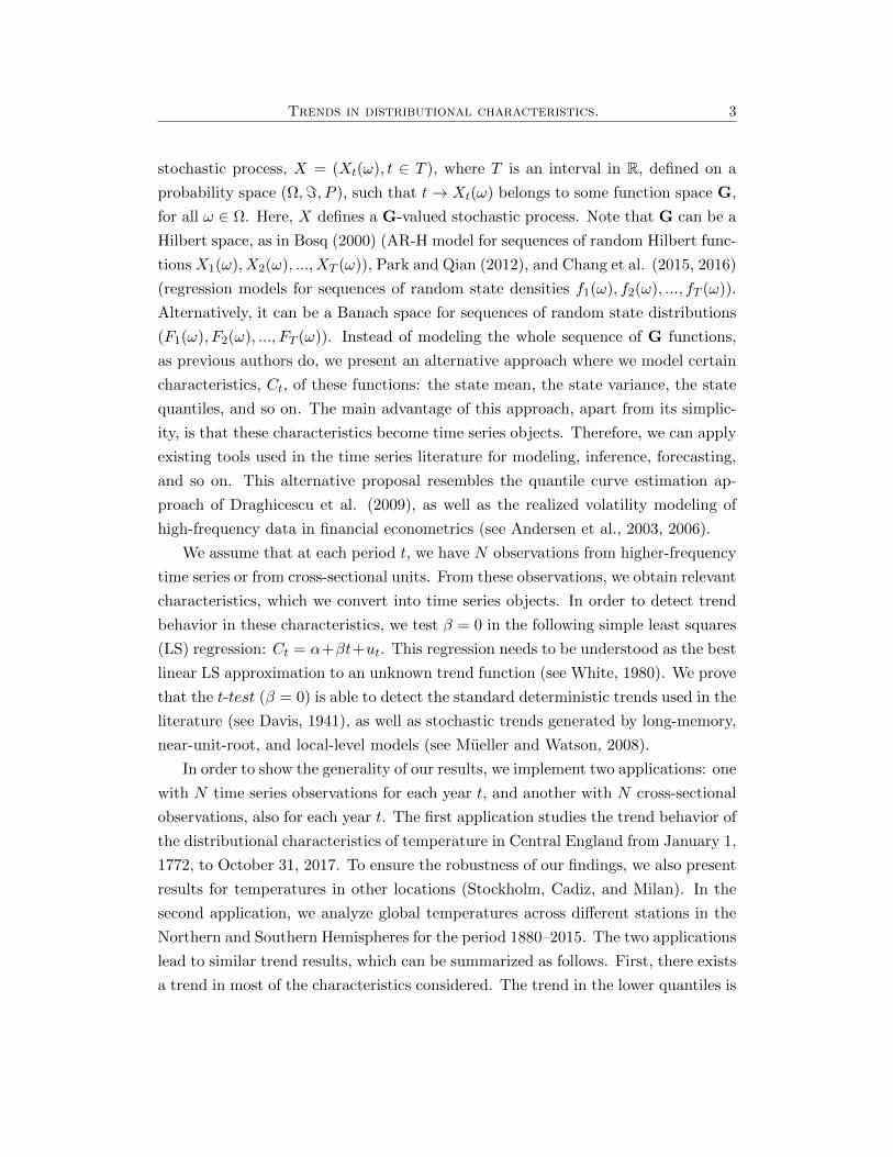
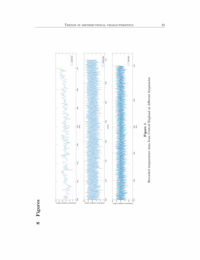
after 1974.3 Figure 1 shows the annual, monthly, and daily versions of the data.4

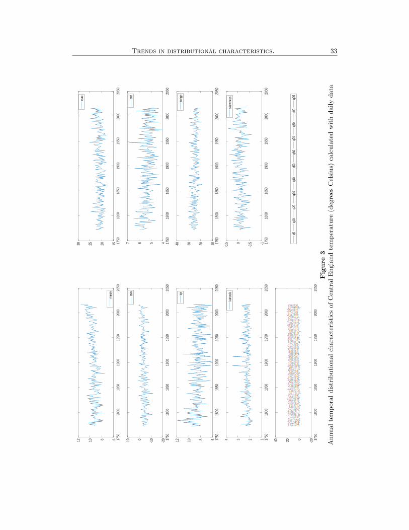
The advantages of the CET climate database are its length and its high fre-

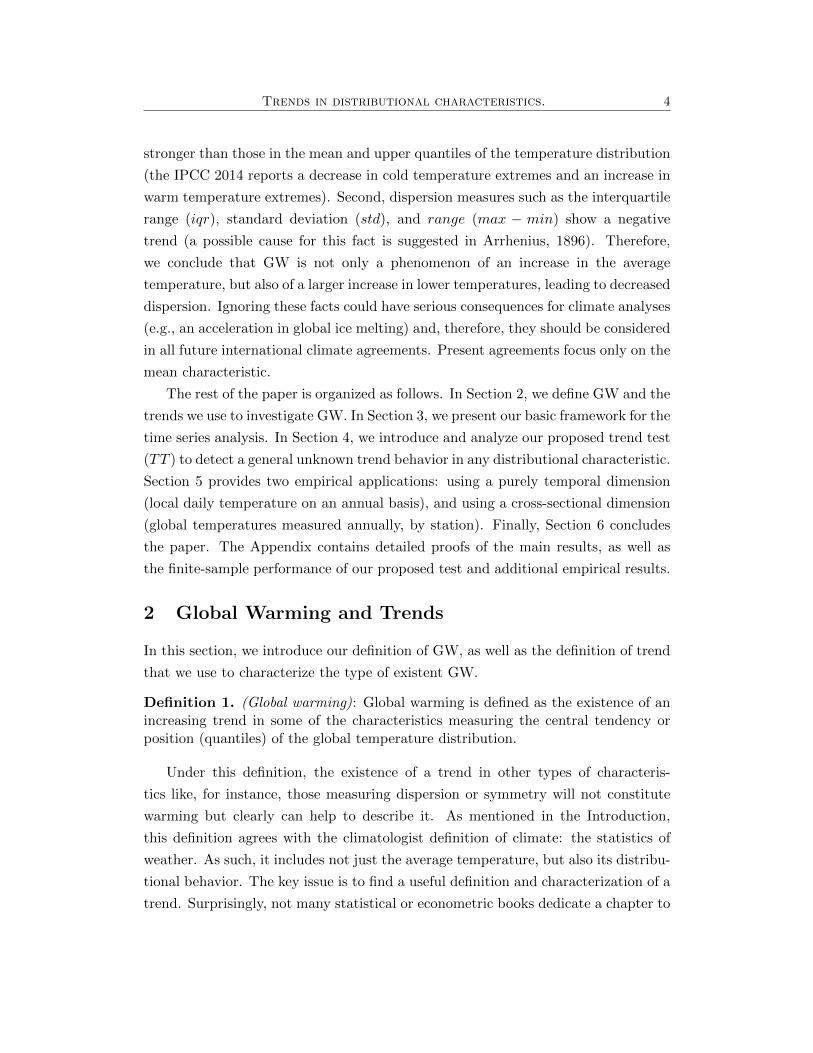
quency. In particular, having daily observations for each year (1772–2017) allows us

to compute the distributional characteristics of interest and convert them into time

series objects. Figure 2 presents the annual densities from 1772 to 2017, and Figure

3 shows the path of these characteristics.

More recently, a European Union research project (IMPROVE) studied past

climatic variability using early daily European instrumental sources. This project

collected records of temperatures in different European areas, from the Baltic to

the Mediterranean and from the Atlantic to Eastern Europe. IMPROVE’s general

objectives were to assess correction and homogenization protocols for early daily

instrumental records of air temperature and air pressure, but the quality and conti-

nuity of the series are highly heterogeneous, and only the Swedish series (Stockholm)

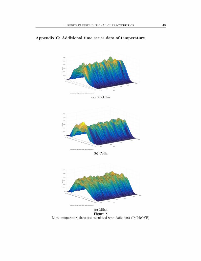
continued to be updated by Anders Moberg.5 In addition to Stockholm, we analyze

data from Cadiz and Milan to test the robustness of our CET results. The density of

the data (Figure 8) and the econometric results for these additional data are shown

in Appendix C.

3See Parker et al. (1992), Manley (1953, 1974), and Parker and Horton (2005) for further infor-mation on these series. The data are available from http://www.metoffice.gov.uk/hadobs/hadcet/.

4An analysis of the statistical properties of the annual and monthly averages of these data canbe found in Harvey and Mills (2003) and in Proietti and Hillebrand (2016).

5They can be obtained from the Bolin Center for Climate Research:http://bolin.su.se/data/stockholm/.


5.1.1 Results

Before testing for the presence of trends in the distributional characteristics of the

CET data, we test for the existence of unit roots. To do so, we use the well-known

Augmented Dickey-Fuller test (ADF; Dickey and Fuller, 1979), where the number

of lags is selected in accordance with the SBIC criterion. The results in Table 1

show that the null hypothesis of a unit root is rejected for all the characteristics

considered.

We test for the presence of a trend in temperature characteristics by applying

the proposed TT in regression (12). Table 2 reports the OLS trend slopes and a

HAC tβ=0 (p-values from a N(0, 1)). The latter indicates a significant trend in all

of the characteristics. The trends are all positive, except those corresponding to the

dispersion measures (std, iqr, range), which are negative. The mean has a trend

coefficient of 0.0038, which implies an increase of 0.4 degrees Celsius in 100 years.

The highest positive trends occur in the lower quantiles. The trend coefficient of the

quantiles ranges from 0.0072 in the 5% quantile (q5) to 0.0013 in the 80% quantile

(q80). Note that this test only confirms the existence of a trend, but says nothing

about its nature. This would require an additional empirical study that determines

the most suitable type of trend. However, this is beyond the scope of this study,

and forms part of on-going research.

These results illustrate the usefulness of our proposed methodology in terms of

analyzing a wide set of distributional characteristics of the temperature instead of

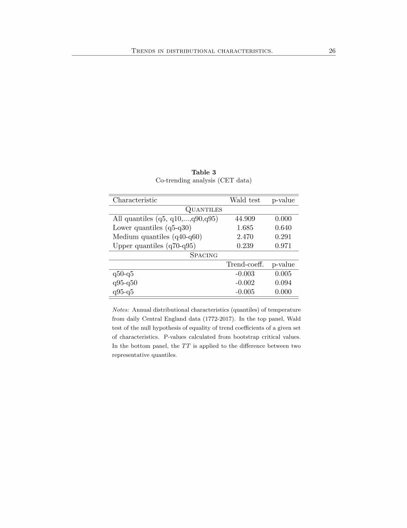
the mean only. To strengthen this idea, we test for co-trending in different sets

of characteristics. The results of a Wald test for different co-trending possibilities

appear in Table 3. The null hypothesis of co-trending in all quantiles is rejected.

Nevertheless, this is not the case if we test the null of equal trends in groups of

quantiles, namely, the lower, medium, and upper quantiles. Finally, to complete

this study, we test for the existence of a trend in important spacing characteris-

tics, and find that the difference between the lowest quantile (q5) and the median

shows a decreasing and significant trend. However, the difference between the high-

est quantile (q95) and the median does not show a statistically significant trend.

The minimum temperatures approach the median more rapidly than the maximum

temperatures do. This is corroborated by a negative trend in q95− q5, and is in line

with the IPCC 2014 summary that reports that winters have warmed more than

summers have.


To close this section, we conduct a parallel study using temperature data for

the other cities mentioned previously: Stockholm, Cadiz, and Milan (see Figure 8).

The results in Table 11 for the unit roots and the trend analysis in Tables 12, 13,

and 14 lead to the same conclusions. Summarizing our findings, we have identified

patterns in the distributional characteristics of temperatures that are common for

different cities with different geographic positions. This infers that this may be a

global phenomenon. The next section investigates this conjecture in further detail.

5.2 Cross-sectional data: GW

The Climate Research Unit (CRU) offers monthly and yearly data of land and sea

temperatures in both hemispheres from 1850 to the present, collected from different

stations around the world.6 Each station temperature is converted to an anomaly,

taking 1961–1990 as the base period,7 and each grid-box value, on a five-degree grid,

is the mean of all the station anomalies within that grid box.8 This database (in

particular, the annual temperature of the Northern Hemisphere) has become one of

the most widely used to illustrate GW from records of thermometer readings. These

records form the blade of the well-known “hockey stick” graph, frequently used by

academics and other institutions, such as, the IPCC. In this paper, we prefer to

base our analysis on raw station data (see density in Figure 4). These data show

high variability at the beginning of the period, probably due to the few number of

stations in this early stage of the project, as noted by Jones et al. (2012). Following

6HadCRUT4 is a global temperature data set, providing gridded temperature anomalies acrossthe world, as well as averages for the hemispheres and for the globe as a whole. CRUTEM4 andHadSST3 are the land and ocean components of this overall data set, respectively. These data setswere developed by the Climatic Research Unit (University of East Anglia) in conjunction with theHadley Centre (UK Met Office), with the exception of the sea surface temperature (SST) data set,which was developed solely by the Hadley Centre. We use CRUTEM version 4.5.0.0, which canbe downloaded from (https://crudata.uea.ac.uk/cru/data/temperature/). A recent revision of themethodology can be found in Jones et al. (2012).

7To avoid biases from the different elevations of stations, monthly average temperatures arereduced to anomalies from the period with best coverage (1961–1990). Because many stations donot have complete records for the period 1961–1990, they are estimated using neighboring recordsor using other sources of data.

8Today, many other institutions collect climate and temperature data. These include the Na-tional Oceanic and Atmospheric Administration (NOAA), which presents daily and monthly rawtemperature data, classified by country and station, from 1961 to the present, and the NationalAeronautics and Space Administration (NASA) offers raw monthly data for stations, anomaliesfor countries, and a method of homogenization of station data since 1880. Furthermore, BerkeleyUniversity offers raw monthly data for stations and anomalies for countries for land temperaturessince 1750, for land and ocean temperatures since 1850, and experimental daily land data since1880.


these authors, our study period begins in 1880 and ends in 2015 (2016 and 2017

data are still under revision).9

The construction of the characteristics deserves a little attention. Although

there are over 10,000 stations on record, the effective number fluctuates each year.

It reached a minimum in 1850 and a maximum during the period 1951–2010. Fur-

thermore, the geographic distribution of stations is not homogeneous. Coverage

is denser over the more populated parts of the world, particularly in the United

States, Southern Canada, Europe, and Japan. In contrast, coverage is sparser over

the interior of the South American and African continents and over Antarctica. This

provokes a disequilibrium between the Northern Hemisphere (NH) and the Southern

Hemisphere (SH). To guarantee the stability of the characteristics over the whole

sample, we select only those stations with data for all years in the sample period,

which forces us to reduce the sample size. Applying this procedure to the sample

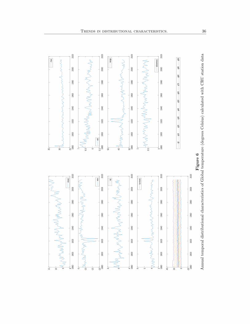
period 1880–2015, we have N=290 stations. Figure 5 shows where they are situated

on a world map, and Figure 6 shows the distributional characteristics as time series

objects. These characteristics are constructed from stations’ annual averages, cal-

culated using monthly temperature records. Note that a benefit of using stable raw

station data is that we always have perfect knowledge of every observation, and can

easily detect the origin of any extreme observations or outliers.10

This method of building characteristics has consequences that should be men-

tioned. The mean calculated from the filtered raw data does not match that reported

by the CRU, which is calculated as the weighted average of all non-missing, grid-

box anomalies in each hemisphere. The weights used are the cosines of the central

latitudes of each grid box, and the global average is a weighted average of those of

the NH and the SH. These weights are “two” for the NH and “one” for the SH.

Therefore, we carry out an additional study using data grids to show that the key

results do not change (results available upon request).

In summary, we analyze raw global data (stations instead of grids) for the period

9Raw station data can present other homogenization problems. Therefore, in addition to carryingout data cleansing, we investigate in detail the controls imposed by the CRU in order to identifyand correct significant inhomogeneities (Jones et al., 2012).

10Figure 6 shows four outliers, which are the result of the way in which annual means are con-structed. Two Russian stations around latitude 51 (codes 308790 and 313690) have few observationsin the central months of the year in 1919 and 1924. For most of the stations considered, there areobservations every, or almost every month. Therefore, the annual average is representative. Wehave verified the robustness of our results in two ways: eliminating the stations causing the outliers,and interpolating the missing values. The results do not change. Therefore, we use the original rawstation data.


1880 to 2015. However, for reasons of homogeneity and stability, we use only data

from stations that are represented in the whole sample period.

5.2.1 Results

The ADF test rejects the null hypothesis of a unit root for all of the characteristics

(see Table 4), with the exception of q80. The unit-root analysis has been completed

in two ways. First, we applied the ADF test station by station, and counted the

number of rejections. Second, we carried out a battery of panel unit-root tests. The

results shown in Table 5 reinforce the conclusion of no unit roots in our temperature

data. Similar unit-root test results are obtained from stable grid data.11

The results change if we include all existing grids in each year (whether they have

observations or not during the whole sample). In this case, we cannot reject the null

of a unit root in many of the annual characteristics, including the mean.12 This is

consistent with the widespread belief that the global temperature has a unit root, a

result that comes from an analysis of the annual mean temperature in the Northern

Hemisphere (see Kaufmann et al., 2006, 2010, 2013). Nevertheless, this result is not

maintained either at monthly frequency (Global, NH and SH), or individually grid

by grid, (84% of the times the unit root is rejected)(results available upon request).

Therefore, it seems that the unit root found in some part of the literature can be a

consequence of temporal or spatial aggregation that produces artificial persistence

(see Taylor, 2001). Other researchers (see Gay-Garcıa et al., 2009; Estrada et al.,

2013) attribute the non-stationarity to the presence of structural breaks in the de-

terministic trend.13 In both cases, TT is able to detect the existence of a trend (see

Propositions 2 and 3.)

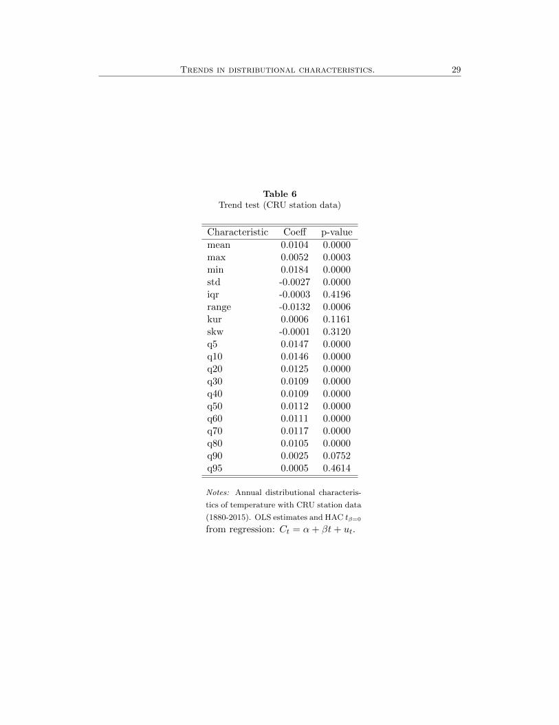
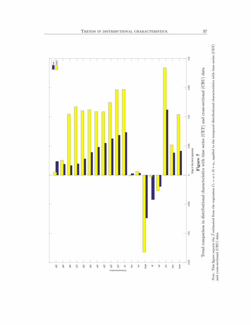
Finally, we apply TT to the characteristics calculated using the cross-sectional

data. The results, displayed in Table 6, lead to the same conclusions obtained from

the distributional characteristics of the time series data.14 This similarity is evident

in Figure 7, which compares the trend slope coefficients estimated from the time-

11Following the same logic as for our station data, we consider only those grids that are repre-sented in the whole sample period. This yields a total of 160 grids.

12Using the same data and following a pure functional approach, Chang et al. (2015) find someevidence of unit-root behavior in some moments. Nevertheless, a panel unit-root test based on allthe grids rejects the unit-root hypothesis (results available upon request).

13In this study, we have not considered structural breaks because they are model dependent andour approach is not. We focus only on detecting the existence of a trend, not on the nature of thetrend.

14This similarity can be extended to the analysis of co-trending, (Table 7), although we rejectthat upper quantiles have the same trend coefficients.


series and the cross-sectional analyses. This finding endorses the behavior patterns

of temperature distribution as a global phenomenon. In summary, we find trends in

most of the Cit (i = 1, ..., p) considered, and they are stronger for the lower quantiles

than they are for the mean and upper quantiles. Dispersion measures such as iqr,

std, and range show a negative trend. Therefore, we conclude that GW is not only

a phenomenon described by an increase in the average temperature, but also one of

a larger increase in the lower quantiles, producing a decreasing dispersion.

6 Conclusion

This study proposes a novel approach to modeling the evolution of certain distribu-

tional characteristics of a functional stochastic process (moments, quantiles, etc.).

This is possible because these distributional characteristics can be obtained as time

series objects and, therefore, we can apply existing tools (modeling, inference, fore-

casting, etc.) available in the time series literature. We present a simple robust trend

test that is able to detect unknown trend components in any of these characteristics.

By defining GW as the existence of an increasing trend in the characteristics

measuring the central tendency or position (quantiles) of the temperature distribu-

tion, testing for a trend is equivalent to testing for the existence of GW, and even

more important, for the type of GW we have.

We apply our methodology to two types of data: (i) time series distributional

characteristics, measured in Central England; and (ii) the global Earth tempera-

ture, with cross-sectional distributional characteristics. In both cases, we obtain the

same conclusions: (i) there is a trend component in all the distributional character-

istics of interest, and this trend is stronger in the lower quantiles than it is in the

mean, median, and upper quantiles; and (ii) the distributional characteristics that

capture the dispersion of the temperature have a negative trend (lower quantiles

evolve toward the median faster than the upper quantiles do). Therefore, there is

clear evidence of local (CET) and global (Earth surface) warming. This warming is

stronger in the lower temperatures than in the rest of the distribution. This result

can have very serious consequences, such as an acceleration of the ice melting pro-

cess. Future international climate agreements should consider this, and not focus

only on the mean temperature.

Note that the proposed trend test is able to detect the existence of an unknown

trend, but not the nature of the trend component. This provides two directions for


future research: (i) modeling the correct trend, and developing methods to forecast

this trend component; and (ii) finding the causes of these distributional trends (see

Arrhenius, 1896).

References

[1] Andersen, T.G., Bollerslev, T., Diebold, F.X., Labys, P., 2003. Modeling and

forecasting realized volatility. Econometrica 71, 529-626.

[2] Andersen, T.G., Bollerslev, T., Christoffersen, P., Diebold, F.X., 2006. Volatil-

ity and correlation forecasting. In: Elliott, G., Granger, C.W.J., Timmermann,

A., eds. Handbook of Economic Forecasting. Amsterdam: North-Holland, 778-

878.

[3] Anderson, T.W., 1971. The Statistical Analysis of Time Series. John Wiley &

Sons, Inc.

[4] Arrhenius, S., 1896. On the influence of carbonic acid in the air upon the

temperature of the ground. Philosophical Magazine and Journal of Science, S5,

Vol 41, No. 251.

[5] Berenguer-Rico, V., Gonzalo, J., 2014. Summability of stochastic processes- A

generalization of integration and co-integration valid for non-linear processes.

Journal of Econometrics 178, 331-341.

[6] Bosq, D., 1998. Nonparametric Statistics for Stochastic Processes. New York:

Springer.

[7] Bosq, D., 2000. Linear Processes in Function Spaces. Lecture Notes in Statistics

149. New York: Springer.

[8] Breitung, J., 2000. The local power of some unit root tests for panel data, in B.

Baltagi (ed.), Advances in Econometrics, Vol. 15: Nonstationary Panels, Panel

Cointegration, and Dynamic Panels, Amsterdam: JAI Press, 161-178.

[9] Breunig, R. V., 2001. Density Estimation for clustered data. Econometrics Re-

views 20(3), 353-367.


[10] Canjels, E., Watson, M.W., 1997. Estimating deterministic trends in the pres-

ence of serially correlated errors. The Review of Economics and Statistics 79,

184-200.

[11] Chang, Y., Kim, Ch.S., Miller, J.I., Park, J.Y., Park, S., 2015. Time series

analysis of global temperature distributions: identifying and estimating per-

sistent features in temperature anomalies. Working Paper 15-13, University of

Missouri.

[12] Chang, Y., Kim, Ch.S, Park, J.Y., 2016. Nonstationarity in time series of state

densities. Journal of Econometrics 192, 152-167.

[13] Choi, I., 2001. Unit root tests for panel data. Journal of International Money

and Finance 20, 249-272.

[14] Dahlhaus, R., 2009. Local inference for locally stationary time series based on

the empirical spectral measure. Journal of Econometrics 151, 101-112.

[15] Davis, H., 1941. The Analysis of Economic Time Series, The Principia Press.

[16] Degenhardt, H.J.A., Puri, M.L., Sun, S., Van Zuijlen, M.C.A., 1996. Charac-

terization of weak convergence for smoothed empirical and quantile processes

under ϕ-mixing. Journal of Statistical Planning and Inference 53, 285-295.

[17] Dickey, D.A., Fuller, W.A., 1979. Distribution of the estimators for autoregres-

sive time series with a unit root. Journal of the American Statistical Association

74, 427-431.

[18] Draghicescu, D., Guillas, S., Wu, W.B., 2009. Quantile curve estimation and vi-

sualization for nonstationary time series. Journal of Computational and Graph-

ical Statistics 18, 1-20.

[19] Durlauf, S.N., Phillips, P.C.B., 1988. Trends versus random walks in time series

analysis. Econometrica 56, 1333-1354.

[20] Embrechts, P., Kluppelberg, C., Mikosh, T., 1999. Modelling Extremal Events

for Insurance and Finance. Springer-Verlag, Berlin.

[21] Estrada, F., Perron, P, Gay-Garcıa C., Martınez-Lopez, B., 2013. A time-series

analysis of the 20th century climate simulations produced for the IPCCs Fourth

Assessment Report. PLoS ONE 8, e60017.


[22] Gay-Garcıa C, Estrada F, Sanchez A., 2009. Global and hemispheric tempera-

tures revisited. Climate Change 94, 333-349.

[23] Grenander, U., Rosenblatt, M., 1957. Statistical Analysis of Stationary Time

Series. New York: Wiley.

[24] Hamilton, J., 1994. Time Series Analysis. Princeton University Press.

[25] Hansen, B.E., 2008. Uniform convergence rates for kernel estimation with de-

pendent data. Econometric Theory 24, 726-748.

[26] Harvey, D.I., Mills, T.C., 2003. Modelling trends in Central England tempera-

tures. Journal of Forecasting 22, 35-47.

[27] Hendry, D.F., Pretis, F., 2013. Some fallacies in econometric modelling of cli-

mate change. Department of Economics. Oxford University. Discussion Papers

643.

[28] Im, K.S., Pesaran, M.H., Shin, Y., 2003. Testing for unit roots in heterogeneous

Panels. Journal of Econometrics, 115, 53-74.

[29] IPCC, 2014. Climate Change 2014: Synthesis report. contribution of working

groups I, II and III to the Fifth Assessment Report of the Intergovernmental

Panel on Climate Change. [Core Writing Team, R.K. Pachauri and L.A. Meyer

(eds.)]. IPCC, Geneva, Switzerland.

[30] Johansen, S., 1995. Likelihood-based Inference in Cointegrated Vector Autore-

gressive Models. Oxford: Oxford University Press.

[31] Jones, P.D., Lister, D.H., Osborn, T.J., Harpham, C., Salmon, M., Morice,

C.P., 2012. Hemispheric and large-scale land surface air temperature variations:

an extensive revision and an update to 2010. Journal of Geophysical Research

117, 1-29.

[32] Kaufmann, R.K., Kauppi, H., Stock, J., 2006. Emissions, concentrations &

temperature: a time series analysis. Climatic Change 77, 249-278.

[33] Kaufmann, R.K., Kauppi, H., Stock, J., 2010, Does temperature contain a

stochastic trend? Evaluating conflicting statistical results. Climatic Change

101, 395-405.


[34] Kaufmann, R.K., Kauppi, H., Mann, M.L., Stock, J., 2013. Does temperature

contain a stochastic trend: linking statistical results to physical mechanisms,

Climatic Change 118, 729-743.

[35] Kendall, M.G., Stuart, A., 1983. Advanced Theory of Statistics, Hafner Press,

New York.

[36] Levin, A., Lin, C.F., Chu, C., 2002. Unit root tests in panel data: asymptotic

and finite-sample properties. Journal of Econometrics 108, 1-24.

[37] Maddala, G.S., Shaowen, W., 1999. A comparative study of unit root tests with

panel data and a new simple test. Oxford Bulletin of Economics and Statistics

61, 631-652.

[38] Maddison, A., 2013. The Maddison-Project, http://www.ggdc.net/maddison/

maddison-project/home.htm, 2013 version.

[39] Manley, G. 1953. The mean temperature of Central England, 1698 to 1952.

Quarterly Journal of the Royal Meteorological Society 79, 242-261.

[40] Manley, G., 1974. Central England temperatures: monthly means 1659 to 1973.

Quarterly Journal of the Royal Meteorological Society 100, 389-405.

[41] Marmol, F., Velasco, C., 2002. Trend stationarity versus long-range dependence

in time series analysis. Journal of Econometrics 108, 25-42.

[42] Mills, T.C., 2010. Skinning a cat: alternative models of representing tempera-

ture trends. An editorial comment. Climate Change 101, 415-426.

[43] Mueller, U.K., Watson, M., 2008. Testing models of low-frequency variability.

Econometrica 76, 979-1016.

[44] Newey, W.K., West, K.D., 1987. A Simple positive semi-definite, hetereko-

dasticity and autocorrelation consistent covariance matrix. Econometrica 55,

703-708.

[45] Park, J.Y., Qian, J., 2012. Functional regression of continuous state distribu-

tions. Journal of Econometrics 167, 397-412.

[46] Parker, D.E., Legg, T.P., Folland, C.K., 1992. A new daily Central England

temperature series, 1772-1991. International Journal of Climatology 12, 317-

342.


[47] Parker, D.E., Horton, E.B., 2005. Uncertainties in the Central England tem-

perature series since 1878 and some changes to the maximum and minimum

series. International Journal of Climatology 25, 1173-1188.

[48] Phillips, P., 2005. Challenges of trending time series econometrics. Mathematics

and Computers in Simulation 68, 401-416.

[49] Proietti, T., Hillebrand, H., 2016. Seasonal changes in Central England tem-

peratures. Journal of the Royal Statistics Society. Statistics in Society. Series

A. (forthcoming).

[50] Silverman, B.W., 1978. Weak and strong uniform consistency of the kernel

estimate of a density and its derivatives. The Annals of Statistics 6, 177-184.

[51] Taylor, A., 2001. Potential pitfalls for the purchasing-power-parity puzzle?

Sampling and specification biases in mean-reversion tests of the law of one

price. Econometrica 69, 473-498.

[52] Vogelsang, T.J., 1998. Trend function hypothesis testing in the presence of

serial correlation. Econometrica 66, 123-148.

[53] White, H., Granger, C.W.J., 2011. Consideration of trends in time series. Jour-

nal of Time Series Econometrics 3, 1-4.

[54] Zhou, Z., Wu, W.B., 2009. Local linear quantiles estimation for nonstarionary

time series. The Annals of Statistics 37, 2696-2729.


7 Tables

Table 1ADF unit root test (CET data)

Characteristic ADF-SBIC p-value lags

mean -8.09 0.000 1max -14.55 0.000 0min -15.13 0.000 0std -16.18 0.000 0iqr -16.44 0.000 0range -16.40 0.000 0kur -16.53 0.000 0skw -13.42 0.000 0q5 -14.28 0.000 0q10 -14.28 0.000 0q20 -14.27 0.000 0q30 -8.89 0.000 1q40 -8.70 0.000 1q50 -8.42 0.000 1q60 -4.94 0.000 3q70 -5.35 0.000 3q80 -14.72 0.000 0q90 -14.47 0.000 0q95 -15.01 0.000 0

Notes: Annual distributional characteristics of temperature

from daily Central England data (1772-2017). Lag-selection ac-

cording to SBIC criterion.


Table 2Trend test (CET data)

Characteristic Coeff p-value

mean 0.0041 0.0000max 0.0038 0.0027min 0.0112 0.0000std -0.0020 0.0000iqr -0.0042 0.0000range -0.0074 0.0000kur 0.0003 0.0552skw 0.0003 0.0682q5 0.0073 0.0000q10 0.0068 0.0000q20 0.0063 0.0000q30 0.0055 0.0000q40 0.0048 0.0000q50 0.0039 0.0000q60 0.0028 0.0009q70 0.0019 0.0127q80 0.0016 0.0240q90 0.0019 0.0346q95 0.0024 0.0145

Notes: Annual distributional character-

istics of temperature from daily Central

England data (1772-2017). OLS estimates

and HAC tβ=0 from regression: Ct =α+ βt+ ut.


Table 3Co-trending analysis (CET data)

Characteristic Wald test p-value

Quantiles

All quantiles (q5, q10,...,q90,q95) 44.909 0.000Lower quantiles (q5-q30) 1.685 0.640Medium quantiles (q40-q60) 2.470 0.291Upper quantiles (q70-q95) 0.239 0.971

Spacing

Trend-coeff. p-value

q50-q5 -0.003 0.005q95-q50 -0.002 0.094q95-q5 -0.005 0.000

Notes: Annual distributional characteristics (quantiles) of temperature

from daily Central England data (1772-2017). In the top panel, Wald

test of the null hypothesis of equality of trend coefficients of a given set

of characteristics. P-values calculated from bootstrap critical values.

In the bottom panel, the TT is applied to the difference between two

representative quantiles.


Table 4ADF unit root test (CRU station data)

Characteristic ADF-SBIC p-value lags

mean -8.04 0.000 0max -5.84 0.000 3min -8.84 0.000 0std -5.46 0.000 1iqr -6.39 0.000 1range -3.53 0.041 3kur -4.24 0.005 3skw -10.20 0.000 0q5 -8.80 0.000 0q10 -8.01 0.000 0q20 -8.75 0.000 0q30 -9.14 0.000 0q40 -9.09 0.000 0q50 -9.15 0.000 0q60 -8.99 0.000 0q70 -8.80 0.000 0q80 -2.66 0.267 3q90 -3.37 0.060 3q95 -3.77 0.021 3

Notes: Annual distributional characteristics calculated from

CRU station data (1880-2015). Lag-selection according to SBIC

criterion.


Table 5Additional unit root analysis (CRU station data)

ADF unit root test by stations

% rejections with all stations 88.99% rejections with NH stations 89.93

Panel unit roots tests

Levin, Lin and Chu -16.50 0.000

Breitung -8.00 0.000

Im, Pesaran and Shin -16.13 0.000

Fisher (ADF) 415.70 0.000

Fisher (PP) 708.46 0.000

Notes: In the top panel, percentage of rejections of the ADF test station

by station, considering all stations from 1880 that have at least 30

observations. In the bottom panel, panel unit root tests of the 19

distributional characteristics. We use the test of Breitung (2000) and

Levin et al. (2002) that assumes common persistence parameters across

cross-sections. Fisher-type tests proposed by Maddala and Wu (1999)

and Choi (2001) and those suggested by Im et al. (2003) allow different

persistence parameters across cross-sections.


Table 6Trend test (CRU station data)


mean 0.0104 0.0000max 0.0052 0.0003min 0.0184 0.0000std -0.0027 0.0000iqr -0.0003 0.4196range -0.0132 0.0006kur 0.0006 0.1161skw -0.0001 0.3120q5 0.0147 0.0000q10 0.0146 0.0000q20 0.0125 0.0000q30 0.0109 0.0000q40 0.0109 0.0000q50 0.0112 0.0000q60 0.0111 0.0000q70 0.0117 0.0000q80 0.0105 0.0000q90 0.0025 0.0752q95 0.0005 0.4614

Notes: Annual distributional characteris-

tics of temperature with CRU station data

(1880-2015). OLS estimates and HAC tβ=0

from regression: Ct = α+ βt+ ut.


Table 7Co-trending analysis

Characteristic Wald test p-value

Quantiles

All quantiles (q5, q10,...,q90,q95) 33.888 0.000Lower quantiles (q5-q30) 4.718 0.194Medium quantiles (q40-q60) 0.020 0.990Upper quantiles (q70-q95) 19.478 0.000

Spacing

Trend-coeff. p-value

q50-q5 -0.004 0.007q95-q50 -0.011 0.035q95-q5 -0.014 0.011

Notes: Annual distributional characteristics (quantiles) of temperature

of CRU station data (1880-2015). In the top panel, Wald test of the null

hypothesis of equality of trend coefficients of a given set of characteris-

tics. P-values calculated from bootstrap critical values. In the bottom

panel, the TT is applied to the difference between two representative

quantiles.


8Figures 16

5917

0817

5818

0818

5919

0819

5820

17

year

s

6789101112 temperature in degrees Celsius

year

ly d

ata

1659

1708

1758

1808

1859

1908

1958

2017

mon

ths

-505101520 temperature in degrees Celsius

Mon

thly

dat

a

1772

1808

1859

1908

1958

2017

days

-20

-100102030

temperature in degrees Celsius

Dai

ly d

ata

Fig

ure

1R

ecor

ded

tem

per

atu

red

ata

from

Cen

tral

En

gla

nd

at

diff

eren

tfr

equ

enci

es


0

0.02

23.1

120

.09

0.04

2017

17.0

8

density0.06

14.0

619

71

tem

pera

ture

in d

egre

es C

elsi

us (d

aily

obs

erva

tions

)

11.0

5

0.08

1921

8.04

year

s

0.1

5.02

1871

2.01

1821

-1.0

0-4

.02

1772

Fig

ure

2C

entr

al

Engla

nd

tem

per

atu

red

ensi

ties

calc

ula

ted

wit

hd

ail

yd

ata


1750

1800

1850

1900

1950

2000

2050

681012

mea

n

1750

1800

1850

1900

1950

2000

2050

15202530m

ax

1750

1800

1850

1900

1950

2000

2050

-20

-10010

min

1750

1800

1850

1900

1950

2000

2050

4567st

d

1750

1800

1850

1900

1950

2000

2050

681012iq

r

1750

1800

1850

1900

1950

2000

2050

10203040ra

nge

1750

1800

1850

1900

1950

2000

2050

1234ku

rtosis

1750

1800

1850

1900

1950

2000

2050

-1

-0.50

0.5

skew

ness

1750

1800

1850

1900

1950

2000

2050

-2002040

q5q1

0q2

0q3

0q4

0q5

0q6

0q7

0q8

0q9

0q9

5

Fig

ure

3A

nnu

alte

mp

oral

dis

trib

uti

onal

char

act

eris

tics

of

Cen

tral

En

gla

nd

tem

per

atu

re(d

egre

esC

elsi

us)

calc

ula

ted

wit

hd

ail

yd

ata


Fig

ure

4G

lob

al

tem

per

atu

red

ensi

ties

calc

ula

ted

wit

hC

RU

stati

on

data


Fig

ure

5G

eogra

ph

ical

dis

trib

uti

on

of

sele

cted

stati

on

s


1880

1900

1920

1940

1960

1980

2000

2020

891011

mea

n

1880

1900

1920

1940

1960

1980

2000

2020

253035m

ax

1880

1900

1920

1940

1960

1980

2000

2020

-20

-15

-10-5

min

1880

1900

1920

1940

1960

1980

2000

2020

5.56

6.57

std

1880

1900

1920

1940

1960

1980

2000

2020

468iq

r

1880

1900

1920

1940

1960

1980

2000

2020

304050ra

nge

1880

1900

1920

1940

1960

1980

2000

2020

3456ku

rtosis

1880

1900

1920

1940

1960

1980

2000

2020

0

0.51

skew

ness

1880

1900

1920

1940

1960

1980

2000

2020

-2002040

q5q1

0q2

0q3

0q4

0q5

0q6

0q7

0q8

0q9

0q9

5

Fig

ure

6A

nnu

alte

mp

oral

dis

trib

uti

onal

chara

cter

isti

csof

Glo

bal

tem

per

atu

re(d

egre

esC

elsi

us)

calc

ula

ted

wit

hC

RU

stati

ond

ata


-0.0

15-0

.01

-0.0

050

0.00

50.

010.

015

0.02

Slop

e in

the

trend

regr

essio

n

mea

n

max

min

std

iqr

rang

e

kur

skw

q5

q10

q20

q30

q40

q50

q60

q70

q80

q90

q95

Characteristics

time

cros

s

Fig

ure

7T

ren

dco

mp

aris

onin

dis

trib

uti

on

al

chara

cter

isti

csw

ith

tim

ese

ries

(CE

T)

an

dcr

oss

-sec

tion

al

(CR

U)

data

Note.

Th

isfi

gu

rere

port

sth

eβ

esti

mate

dfr

om

the

regre

ssio

nCt

=α

+βt+ut,

ap

plied

toth

ete

mp

ora

ld

istr

ibu

tion

al

chara

cter

isti

csw

ith

tim

ese

ries

(CE

T)

an

dcr

oss

-sec

tion

al

(CR

U)

data

.


Appendix

Appendix A: Proofs

Proof of Proposition 1

See Sections 16.1 and 16.2 in Hamilton (1994).


Part 1: Asymptotic behavior of OLS β:

β =

T∑t=1

(Ct − C)(t− t)

T∑t=1

(t− t)2

=

T∑t=1

Ctt− CT∑t=1

t− tT∑t=1

Ct + Ct

T∑t=1

(t− t)2

(13)

Taking into account that

T∑t=1

Ctt = Op(T2+δ),

CT∑t=1

t = Op(T2+δ),

tT∑t=1

Ct = Op(T2+δ),

Ct = Op(T1+δ)

andT∑t=1

(t− t)2 = O(T 3),

we obtain that β = Op(Tδ−1).

Part 2: Asymptotic behaviour of tβ=0:

tβ=0 =β − 0√

σ2u/

T∑t=1

(t− t)2

=

T∑t=1

(Ct − C)(t− t)√σ2u

T∑t=1

(t− t)2

(14)


From Part 1 the numerator is Op(T2+δ). It is easy to obtain that

σ2u =

T∑t=1

(Ct − α− βt)2

T=

Op(T

(1+2δ−γ) for 0 ≤ γ ≤ 1

Op(T2δ) for 1 ≤ γ ≤ 1 + δ

(15)

Taking into account thatT∑t=1

(t− t)2) = O(T 3), the result follows.


For the fractional case, 1/2 < d < 3/2, see Marmol and Velasco (2002).

For the near unit root as well as for the local level model, the proof follows straight-

forward from the proof in Durlauf and Phillips (1988) for the pure I(1) case.

Appendix B: Finite-sample performance

In this appendix, the finite-sample performance of our proposed trend test (TT )

is analyzed via a Monte Carlo experiment. Sample sizes are T = 200, 500, and

1000. Number of replications is equal to 10,000. In all cases, the significance level

is 5% (critical values for a N(0,1)) and a HAC tβ=0 is used. In general, the pa-

rameters of a given model have been estimated or selected by fitting that model to

the average annual Central England temperature (1772-2015). However, in some

cases (super-exponential trends, Gompertz curves and logistic trends), when the

fitting is very unstable we use other typical economic series such as the UK nominal

GDP per-capita (1800-2010) (from Madisson, 2013) and others (Population, IPI and

Wholesale Prices) from Davis (1941).

SIZE

The empirical size is investigated by generating several non-trending models.

• Case 1: A white noise model (WN) from a Normal (0, 1).

• Case 2: sin(u ∗ t), t = 1, ..., T , u∼ U(0, 1), where u is used to reduce the

frequency of the sin function.

• Case 3: An AR(2) process whose parameter values are obtained from fitting

an AR(2) to the average annual Central England temperature.


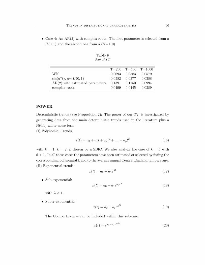
• Case 4: An AR(2) with complex roots. The first parameter is selected from a

U(0, 1) and the second one from a U(−1, 0)

Table 8Size of TT

T=200 T=500 T=1000

WN 0.0693 0.0583 0.0579sin(u*t), u∼ U(0, 1) 0.0582 0.0377 0.0388AR(2) with estimated parameters 0.1391 0.1150 0.0994complex roots 0.0499 0.0445 0.0389

POWER

Deterministic trends (See Proposition 2): The power of our TT is investigated by

generating data from the main deterministic trends used in the literature plus a

N(0,1) white noise term:

(I) Polynomial Trends

x(t) = a0 + a1t+ a2t2 + ....+ apt

k (16)

with k = 1, k = 2, k chosen by a SBIC. We also analyze the case of k = θ with

θ < 1. In all these cases the parameters have been estimated or selected by fitting the

corresponding polynomial trend to the average annual Central England temperature.

(II) Exponential trends

x(t) = a0 + a1eλt (17)

• Sub-exponential:

x(t) = a0 + a1ea2tλ (18)

with λ < 1.

• Super-exponential:

x(t) = a0 + a1eeλt (19)

The Gompertz curve can be included within this sub-case:

x(t) = ea0−a1e−λt

(20)


(III) Logistic Trends

x(t) =a1

1 + a2e−λt(21)

(IV) Segmented Trends

x(t) = a0 + b0d1t + a1t+ b2d1tt (22)

with d1t being a dummy variable that takes the value 1 in regime A and 0 in regime B.

(V) Logistic Smooth Transition Trends

x(t) = a0 + a1t+ (b0 + b2t)St(θ, τ) (23)

with St(θ, τ) = (1 + exp(−θ(t− τT )))−1.

Table 9Power (deterministic trends) of TT

T=200 T=500 T=1000

Polynomial trend k=1 0.9998 1.0000 1.0000Polynomial trend k=2 0.9119 1.0000 1.0000Polynomial trend k=sbic 0.9083 1.0000 1.0000Polynomial trend k = θ < 1 0.9937 1.0000 1.0000Exponential 0.8782 1.0000 1.0000Exponential (sub) 0.8718 1.0000 1.0000Exponential (super, UK GDP) 1.0000 - (*) - (*)Exponential (Gompertz curve, UK GDP) 1.0000 - (*) - (*)Logistic (Population) 1.0000 1.0000 1.0000Logistic (Industrial Production Index) 1.0000 1.0000 1.0000Logistic (Wholesale Prices) 1.0000 1.0000 1.0000Segmented trends 1.0000 1.0000 1.0000Logistic smooth transition (UK GDP) 1.0000 1.0000 1.0000

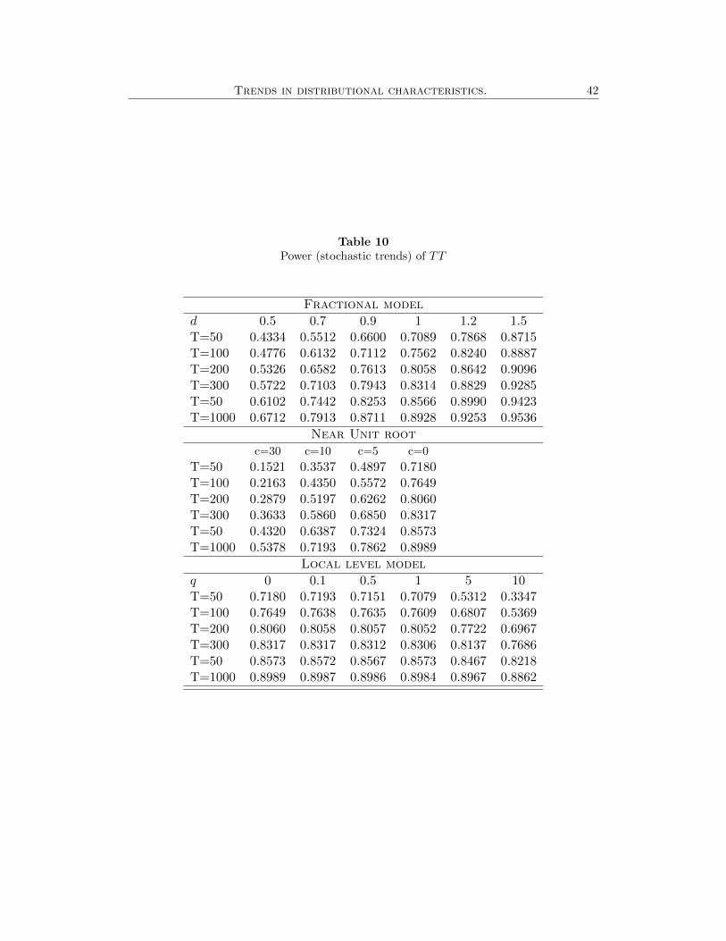
Stochastic trends (see Proposition 3) Following Mueller and Watson (2008) we

consider the three most common long-run models generating stochastic trends: frac-

tional models (1/2 < d < 3/2), near unit root models and local level models.


Table 10Power (stochastic trends) of TT

Fractional model

d 0.5 0.7 0.9 1 1.2 1.5T=50 0.4334 0.5512 0.6600 0.7089 0.7868 0.8715T=100 0.4776 0.6132 0.7112 0.7562 0.8240 0.8887T=200 0.5326 0.6582 0.7613 0.8058 0.8642 0.9096T=300 0.5722 0.7103 0.7943 0.8314 0.8829 0.9285T=50 0.6102 0.7442 0.8253 0.8566 0.8990 0.9423T=1000 0.6712 0.7913 0.8711 0.8928 0.9253 0.9536

Near Unit root

c=30 c=10 c=5 c=0

T=50 0.1521 0.3537 0.4897 0.7180T=100 0.2163 0.4350 0.5572 0.7649T=200 0.2879 0.5197 0.6262 0.8060T=300 0.3633 0.5860 0.6850 0.8317T=50 0.4320 0.6387 0.7324 0.8573T=1000 0.5378 0.7193 0.7862 0.8989

Local level model

q 0 0.1 0.5 1 5 10T=50 0.7180 0.7193 0.7151 0.7079 0.5312 0.3347T=100 0.7649 0.7638 0.7635 0.7609 0.6807 0.5369T=200 0.8060 0.8058 0.8057 0.8052 0.7722 0.6967T=300 0.8317 0.8317 0.8312 0.8306 0.8137 0.7686T=50 0.8573 0.8572 0.8567 0.8573 0.8467 0.8218T=1000 0.8989 0.8987 0.8986 0.8984 0.8967 0.8862


Appendix C: Additional time series data of temperature

0

0.01

24.67

0.02

20.7416.81

0.03

dens

ity

201512.88

0.04

temperature in degrees Celsius (daily observations)

8.95 1955

0.05

5.02

years

1905

0.06

1.081855-2.85

1805-6.78-10.71 1756

(a) Stockolm

0

0.02

31.19

0.04

28.2225.25

0.06

2000

dens

ity

22.27

0.08

1966


19.30

0.1

16.33

years

1916

0.12

13.3510.38 1866

7.404.43 1817

(b) Cadiz

0

0.01

33.33

0.02

28.6323.93 1998

0.03

dens

ity

19.23 1962

0.04


14.53

0.05

19129.84

years

0.06

5.14 18620.44

1812-4.26-8.95 1763

(c) Milan

Figure 8Local temperature densities calculated with daily data (IMPROVE)


Table 11Unit root tests (IMPROVE data)

Characteristic Stockholm Cadiz Milan

mean -13.34 -5.94 -12.77(0.000) (0.000) (0.000)

max -16.96 -8.45 -13.20(0.000) (0.000) (0.000)

min -14.86 -8.97 -13.88(0.000) (0.000) (0.000)

std -13.99 -8.46 -13.94(0.000) (0.000) (0.000)

iqr -14.14 -9.65 -15.07(0.000) (0.000) (0.000)

range -15.88 -11.77 -13.50(0.000) (0.000) (0.000)

kur -17.07 -14.37 -13.81(0.000) (0.000) (0.000)

skw -14.18 -12.57 -13.62(0.000) (0.000) (0.000)

q5 -13.51 -6.28 -14.35(0.000) (0.000) (0.000)

q10 -13.58 -8.38 -14.31(0.000) (0.000) (0.000)

q20 -13.93 -8.13 -13.71(0.000) (0.000) (0.000)

q30 -13.82 -7.79 -14.55(0.000) (0.000) (0.000)

q40 -13.57 -6.76 -13.85(0.000) (0.000) (0.000)

q50 -13.37 -6.91 -13.69(0.000) (0.000) (0.000)

q60 -3.26 -10.61 -8.87(0.076) (0.000) (0.000)

q70 -13.41 -5.82 -13.03(0.000) (0.000) (0.000)

q80 -13.66 -3.41 -5.77(0.000) (0.053) (0.000)

q90 -14.91 -4.11 -6.18(0.000) (0.008) (0.000)

q95 -15.85 -12.06 -13.33(0.000) (0.000) (0.000)

Notes: Annual distributional characteristics of temper-

ature from IMPROVE daily data. Data from Stock-

holm (1756-2012), Cadiz (1817-2000) and Milan (1763-

1998) from Camuffo and Jones (2002). Stockholm tem-

peratures have been updated to 2015 by Bolin Center

Database. P-values in brackets. Lag-selection according

to SBIC criterion.


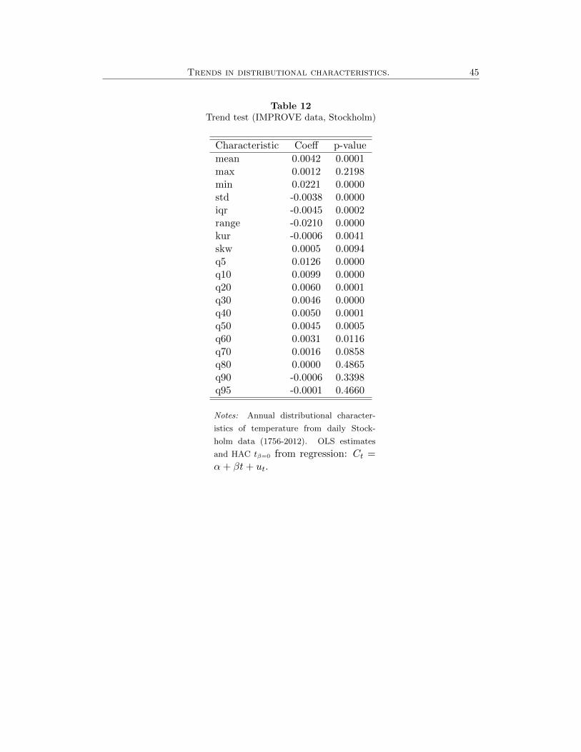
Table 12Trend test (IMPROVE data, Stockholm)


mean 0.0042 0.0001max 0.0012 0.2198min 0.0221 0.0000std -0.0038 0.0000iqr -0.0045 0.0002range -0.0210 0.0000kur -0.0006 0.0041skw 0.0005 0.0094q5 0.0126 0.0000q10 0.0099 0.0000q20 0.0060 0.0001q30 0.0046 0.0000q40 0.0050 0.0001q50 0.0045 0.0005q60 0.0031 0.0116q70 0.0016 0.0858q80 0.0000 0.4865q90 -0.0006 0.3398q95 -0.0001 0.4660

Notes: Annual distributional character-

istics of temperature from daily Stock-

holm data (1756-2012). OLS estimates

and HAC tβ=0 from regression: Ct =α+ βt+ ut.


Table 13Trend test (IMPROVE data, Cadiz)


mean 0.0047 0.0000max 0.0070 0.0042min 0.0070 0.0489std -0.0006 0.2648iqr -0.0000 0.4999range -0.0037 0.0119kur 0.0009 0.0011skw 0.0002 0.2565q5 0.0050 0.0132q10 0.0057 0.0009q20 0.0059 0.0001q30 0.0060 0.0001q40 0.0053 0.0009q50 0.0042 0.0020q60 0.0044 0.0007q70 0.0040 0.0027q80 0.0018 0.0798q90 0.0036 0.0065q95 0.0059 0.0002


tics of temperature from daily Cadiz data




Table 14Trend test (IMPROVE data, Milan)


mean 0.0027 0.0002max 0.0023 0.0679min 0.0120 0.0000std -0.0025 0.0000iqr -0.0058 0.0000range -0.0097 0.0001kur 0.0002 0.0492skw 0.0004 0.0015q5 0.0067 0.0000q10 0.0068 0.0000q20 0.0061 0.0000q30 0.0047 0.0000q40 0.0033 0.0034q50 0.0006 0.3130q60 -0.0008 0.2091q70 -0.0005 0.3253q80 -0.0001 0.4591q90 0.0007 0.2802q95 0.0021 0.0437


tics of temperature from daily Milan data



Documents

Trends in distributional characteristics: Existence of ...jgonzalo/TrendDistributional... · Trends in distributional characteristics: Existence of global warming Mar a Dolores Gadea