TRENDS AND VARIATIONS OF MONTHLY MEAN MINIMUM …eajournals.org/wp-content/uploads/Trends-And-Variations-Of-Monthly... · TRENDS AND VARIATIONS OF MONTHLY MEAN MINIMUM AND MAXIMUM

International Journal of Pure and Applied Physics

Vol.2,No.4, pp.1-27, December 2014

Published by European Centre for Research Training and Development UK (www.eajournals.org)

1

TRENDS AND VARIATIONS OF MONTHLY MEAN MINIMUM AND MAXIMUM

TEMPERATURE DATA OVER NIGERIA FOR THE PERIOD 1950-2012.

S.O. AMADI1*, S.O. UDO2 , AND I.O. EWONA3

1. Dept. of Physics, Geology and Geophysics, Federal University Ndufu-Alike Ikwo,

Ebonyi State.

2. Dept. of Physics, University Of Calabar, Calabar, Nigeria

3. Dept. of Physics, Cross River University of Technology, Calabar, Nigeria.

ABSTRACT: The monthly mean maximum and minimum temperature data were analysed

with the aim of revealing spatial and temporal pattern of long-term trends in the variables. The

study is based on the data collected from Nigeria Meteorological Agency’s network of

meteorological stations spread across Nigeria spanning from 1950-2012. A total of 20

meteorological stations spread across Nigeria were used for the analysis. Statistical techniques

such as time-series plots, correlation analysis, descriptive statistics and Mann-Kendall’s test

were used for the analysis. These analyses were executed using the R programming language,

MATLAB and SPSS computer software packages. The results show latitudinal dependence of

basic temperature characteristics with the northern part of the country exhibiting higher

temperature variability than the south. The Mann-Kendall tests indicate that 17 stations

(representing 85%) show significant increasing trends in the minimum temperature at the 0.01

level of significance while 16 stations (representing 80%) show significant increasing trends

in the maximum temperature at the 0.01 and 0.05 significance levels. Port Harcourt and Ikeja

have greatest trend coefficients among the 20 stations. The minimum temperatures have higher

trend coefficients than the maximum temperatures for almost all the stations. The interstation

spatial coherence revealed by correlation coefficients indicates that almost all the station’s

minimum and maximum temperatures are positively correlated with others at the 0.01 level of

significance. The Mann-Kendall’s test results show a general warming trend across the

stations.

KEYWORDS: Trends, maximum temperature, minimum temperature, Mann-Kendall,

variability, Nigeria.

INTRODUCTION

The global atmosphere is undergoing a period of rapid human – driven change, with no

historical precedent in either its rate of change or its potential absolute magnitude (IPCC, 2002),

in Malhi and Wright (2004). Human activities are continuing to affect the earth’s energy budget

by changing the emissions and resulting atmospheric concentrations of radiatively important

gases and aerosols, and by changing land surface properties. One of the most common

indicators of climate change is the surface air temperature. There are a vast amount of research

papers that examined changes in global and regional mean temperatures over time (Karabulut

et al., 2008, Turkes et al., 2002; Olofintoye and Sule, 2010; Jain and Kumar, 2012; Gil-Alana,

2008; Jones et al., 2013; Ewona and Udo, 2008). Global climate has changed significantly in

the last century. Global mean surface temperature has increased by 0.74oC during the last

century (IPCC, 2007).

http://www.eajournals.org/




2

Trend detection in temperature and precipitation time series is one of the interesting research

areas in climatology. Precipitation and temperature changes are not uniform. Regional

variations can be much larger, and considerable spatial and temporal variations may exist

between climatically different regions (Yue and Hashino, 2003). A number of studies have

evaluated the trends in temperature on different spatial and temporal scales (Ogolo and

Adeyemi, 2009; Odjugo, 2011; Malhi and Wright, 2004; Kiladis and Diaz, 1989; Klein-Tank

and Konnen, 2003).

Climate change over a region would have a significant impact on agricultural production and

related sectors, water resources management and overall economy of the country. Food and

energy security are crucially dependent on the timely availability of adequate amount of water

and a conducive climate. Temperature and its changes impact a number of hydrological

processes including rainfall, and these processes in turn impact temperature e.g cooling due to

rain or snow (Jain and Kumar, 2012; Ewona and Udo, 2011). Today, climate change has direct

effects on increasing global temperature, alter precipitation patterns, alter pattern of agriculture,

increase size and number of forest fires etc (Karaburun et al., (2012). Climate change also has

indirect effects on human health, caused by infectious disasters such as water – borne and

vector – borne disasters, and socio-economic effects caused by environmental change and

ecological disruption (WHO, 2003) in Karaburun et al., (2012). Although regional effects of

climate change vary based on location of regions, there is a growing consensus that

temperatures are on the rise. Analysis of worldwide air temperature changes have shown that

temperature has increased in both northern and southern hemispheres over the last century with

warming more dominant in the northern hemisphere since the 1950s (Rebetez and Reinhard,

2008) in Karaburun et al., (2011).

Many regional studies have also found a positive trend in temperature, although the changes

vary slightly from one region to another (Abatzoglou et al, 2009; Karaburun et al, 2011;

Ustaoglu, 2012; Liu et al., 2006; Abudaya, 2013; Karaburun et al., 2012). Urbanization makes

significant changes in the surface parameters which have the potential to change the local

climate in cities (Ezber et al, 2007) in Ustaoglu (2012). Ustaoglu (2012) further posited that

population growth and urbanization have warming effect on climates. A number of different

methods have been used to evaluate the changes in mean, maximum and minimum

temperatures with changing pattern from region to region (Duffy et al., 2001; Peterson and

Vose 1997; Jones and Moberg, 2003; Karaburun et al, 2012; Sonali and Kumar (2013). Several

parametric and non-parametric statistical tools are used to analyze trends in climate change

studies. Mann-Kendall trend test, Sen’s slope estimator and spearman’s rank order correlation

tests are used to analyze the direction, magnitudes and significance of possible trends in

observed data.

The current goal of applied climate science is to improve knowledge at regional and local

levels. The smaller the scale at which information can be provided, the greater the relevance to

users for most applications. Therefore, the basic objectives of the study are:

I To infer the nature of spatial and temporal variations of minimum and maximum

temperature over Nigeria from 1950 – 2012 period using 20 synoptic stations.

II To examine the trends of monthly mean minimum and maximum temperatures from

1950 – 2012 for the 20 synoptic stations spread across Nigeria.





3

Trends have become the most commonly used technique to detect climatic variability in

regional and local basis. In this study, Mann-Kendall’s rank correlation test and other statistical

tools were used. Some trend studies in instrumental records of temperature have been

conducted in Nigeria, the most comprehensive being Abiodun et al, (2011) which covered a

period of 30 years (1971 – 2000) in 40 weather stations across Nigeria. This study extended

the evaluation of temperature trends to cover a period of 63 years (1950 – 2012) for 90% of the

stations selected for the study.

STUDY AREA

Nigeria lies between latitude 40N and 14oN, and between longitude 20E and 15oE. It coordinates

on 10.00oN and 8.00oE. It has a total area of 923.77km2 and land mass coverage of 910.77km2.

Nigeria is composed of various ecotypes and climatic zones, defining different temperature

regimes. The Nigerian climate is dominated by the influence of the Tropical Maritime (TM)

air mass and the Tropical Continental (CT) air mass. The TM air mass originates from the

southern high-pressure belt located off the Namibian Coast, which then picks up moisture from

over the Atlantic Ocean, thus becoming a moisture – laden air mass (Abiodun et al, 2011). The

CT air mass originates from the high pressure belt, north of the Tropic of Cancer and is always

dry. It travels towards Nigeria over the Sahara desert. The TM and CT air masses converge at

a place called the Inter Tropical Convergence Zone (ITCZ) also called the Inter Tropical

Discontinuity (ITD). The seasonal northward and southward migration of the ITD dictates the

weather pattern of Nigeria. Figure 1 is Map of Nigeria showing the locations of the stations

used in the study.

Fig 1: Map of Nigeria showing meteorological locations for the study

N





4

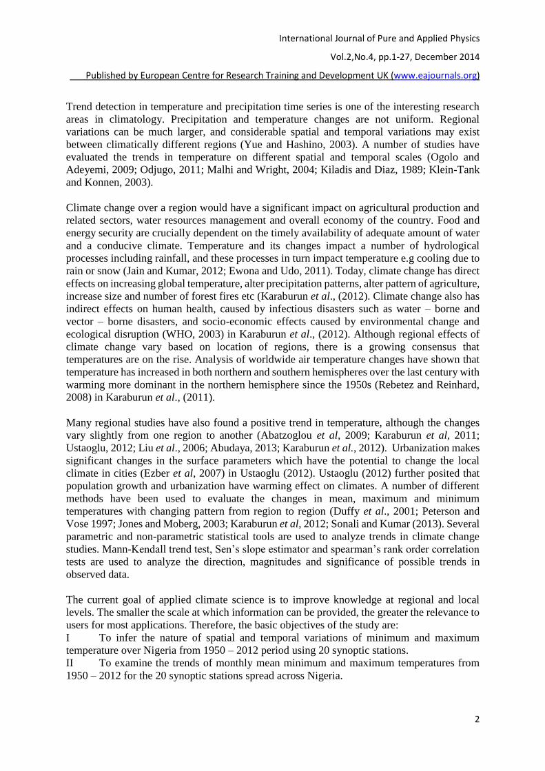
THE DATA

Monthly mean values of daily minimum and maximum temperatures for the period 1950 –

2012 at 20 synoptic stations spread across Nigeria were obtained from the archives of the

Nigerian Meteorological Agency, (NIMET) Oshodi, Lagos, Nigeria. Table 1 below gives the

details of the station locations and the data length.

Table 1: Description of weather stations and data used

Station

No

Station Name Latitude

(oN)

Longitude

(oE)

Elevation

(m)

Period Sequence length

(month)

Max T Min T

1. Yelwa 10.53 4.45 244 1950 - 2012 756 756

2 Sokoto 12.55 5.12 351 1950 - 2012 756 756

3 Kaduna 10.42 7.19 645 1950 - 2012 756 756

4 Kano 12.03 8.32 476 1950 - 2012 756 756

5 Bauchi 10.17 9.49 591 1950 - 2012 756 756

6 Maiduguri 11.51 13.05 354 1950 - 2012 756 756

7 Ilorin 8.26 4.3 308 1950 - 2012 756 756

8 Yola 9.16 12.26 191 1950 - 2012 756 756

9 Ikeja 6.35 3.2 40 1950 - 2012 756 756

10 Ibadan 7.22 3.59 234 1950 - 2012 756 756

11 Oshogbo 7.47 4.29 305 1950 - 2012 756 756

12 Benin 6.19 5.36 77.8 1950 - 2012 756 756

13 Warri 5.31 5.44 6 1950 - 2012 756 756

14 Lokoja 7.48 6.44 113 1950 - 2012 756 756

15 Port Harcourt 5.01 6.57 18 1950 - 2012 756 756

16 Owerri 5.25 7.13 91 1974 – 2012 444 468

17 Enugu 6.28 7.34 142 1950 - 2012 756 756

18 Calabar 4.58 8.21 62 1950 - 2012 756 756

19 Makurdi 7.42 3.37 113 1950 - 2012 756 756

20 Ogoja 6.4 8.48 117 1976 – 2012 444 444

METHODOLOGY

Data Check and Smoothening

Quality check was carried out on the data. Only the Owerri data have missing values of 24

months in maximum temperature which represents 5% of the data length. Missing entries were

not replaced as there were no nearby enough stations to help in estimating them. Shongwe et

al, (2006) suggested the use of data from stations with missing values not exceeding 5%.

Ngongondo et al (2011) recommended the use of data with up to 10% missing entries for cases

of data scarce region. The stations’ meta data were not available. Inhomogeneities observed

were very likely related to the long term fluctuations and trends, which are accepted within

other non-randomness characteristics of the series of climatological observations (Syners,

1990; Turkes, 1999). The data were smoothened by the moving average technique to get rid of

fluctuations.





5

DATA PROCESSING

SPSS computer software package was used to evaluate the descriptive statistics of the

temperature distributions to reveal the minimum and maximum temperature characteristics of

the stations. The Bar charts were produced to give the seasonal variation of temperature of the

stations over the entire period using the R programming language. The Pearson’s Product

moment correlation coefficients were carried out using the SPSS computer package to give the

spatial correlations of the minimum and maximum temperatures of the stations. The Time

series plots with trend lines were done using MATLAB software. The non-parametric Mann-

Kendall’s test was applied to detect trend direction and trend significance. The non-parametric

Mann-Kendall’s test is superior to the parametric tests (Karaburun et al, 2011; Ustaoglu, 2012;

Karabulut, 2008) because Mann-Kendall test allows for missing values in time series data; it

does not require to conform to any particular distribution; and it is robust to the effect of outliers

(single data errors) (Turkes, 1999).

The Mann-Kendall’s Rank Correlation Test

For n size data set such that n ≥ 10, and assuming that the time series is independent, the Mann-

Kendall’s test statistic S is calculated according to the following formula.

)1(sgn1

1

1

kx

jxS

n

kj

n

k

where xj and xk are the sequential data for the ith and jth terms, where j>k.

01

)2(00

01

sgn

kj

kj

kj

kj

xxif

xxif

xxif

xx

A high positive value of S is an indicator of increasing trend while a large negative value of S

is an indicator of decreasing tend. The variance of S, VAR(S), where there are no ties (ie j=k

does not exist) is computed as

VAR=

In the presence of ties, VAR(S) is expressed thus:





6

VAR (S) )4()52)(1()52)(1(

18

1

1

q

p

ppp tttnnn

q is the number of tied groups (where j = k) and tp is the number of data values in the pth group.

The values of S and VAR(S) are used to compute the test statistic Z as:

0

)5(00

0

)(

1

)(

1

Sif

Sif

Sif

Z

SVAR

S

SVAR

S

Z follows a normal distribution.

The null hypothesis Ho for a two-tailed test is that there is no trend, and that the data are

randomly ordered. The alternative hypothesis H1 is that there is a trend. The null hypothesis is

rejected when the Z value determined by eqn (5) is greater in absolute value than the critical

(table) value Zα/2 at the α level of significance, ie /Z/ > Zα/2. Otherwise the null hypothesis is

not rejected. The Z value is tested at 5% and 1% levels of significance. The trend is positive

(increasing) if Z is positive and negative (decreasing) if Z is negative.

In statistics, the Kendall rank correlation coefficient, commonly referred to as Kendall’s tau

coefficient, is a statistic used to measure the association between two quantities. A tau test is a

non-parametric hypothesis test for statistical dependence based on the tau coefficient. Values

of tau b statistic range from -1 (100% negative association, or perfect inversion) to +1 (100%.

positive association, or a perfect agreement). A value of zero indicates the absence of

association.

The P – Value

The p – value gives the area in the tails of the probability density beyond the observed value of

the test static. If a particularly large value for the test statistic is observed, then the p – value

will be very small. The null hypothesis is rejected if the p-value is less than the chosen level of

significance, α (ie p-value <α) on the ground that the data are inconsistent with the null

hypothesis at the chosen level of significance α. Otherwise, the null hypothesis is not rejected

since the data are consistent with it.

RESULTS AND DISCUSSION

Table 2a shows the descriptive statistics for minimum temperature. The coefficient of variation

(C.V) and the mean show latitude dependence, the C.V being higher at higher latitudes (in the

north) and vice verse for the mean. The north shows higher variability in minimum temperature





7

than the south. Maiduguri, followed by Kano have highest values of the coefficient of variation

while Calabar has the least. Table 2b shows the descriptive statistics for maximum temperature.

The C.V and the mean are also latitude dependent decreasing from higher latitudes (in the

north) to lower latitudes (in the south). A cursory

Table 2a – Descriptive Statistics for Minimum Temperature Station N Minimum Maximum Mean Std. Deviation Range CV(%)

Yelwa 756 11.10 28.10 21.2851 3.61501 17.00 17.00

Sokoto 756 12.80 29.00 21.8480 3.55526 16.20 16.29

Kaduna 756 11.20 28.90 19.7415 3.11623 17.70 15.81

Kano 756 10.40 26.50 19.7167 3.86243 16.10 19.57

Bauchi 756 9.20 25.90 19.0515 3.44857 16.70 18.11

Maidugiri 756 9.20 34.00 19.9503 4.58402 24.80 22.96

Ilorin 756 11.30 26.20 21.2438 1.67346 14.90 7.86

Yola 756 11.50 29.00 21.8795 3.18133 17.50 14.53

Ikeja 756 16.00 27.80 23.0131 1.27311 11.80 5.52

Ibadan 756 16.40 30.90 22.0951 1.25940 14.50 5.70

Oshogbo 756 13.50 25.70 21.3563 1.62221 12.20 7.59

Benin 756 18.40 32.50 22.7183 1.43535 14.10 6.34

Warri 756 19.30 32.70 23.1000 1.02641 13.40 4.46

Lokoja 756 14.10 33.60 22.8163 2.02941 19.50 8.90

P/ Harcourt 756 14.90 29.50 22.4712 1.12377 14.60 4.98

Owerri 468 17.80 28.10 23.2021 1.10283 10.30 4.74

Enugu 756 16.10 26.50 22.2706 1.38727 10.40 6.24

Calabar 756 20.10 29.70 22.9217 .85390 9.60 3.71

Makurdi 756 13.30 31.70 22.1820 2.39077 18.40 10.78

Ogoja 444 15.90 29.30 22.3829 1.61484 13.40 7.19

Table 2b – Descriptive Statistics for Maximum Temperature Station N Minimum Maximum Mean Std. Deviation Range CV (%)

Yelwa 756 28.4 41.1 34.526 2.9531 12.7 8.45

Sokoto 756 21.7 42.2 35.094 3.2697 20.5 9.32

Kaduna 756 21.7 38.0 31.572 2.6273 16.3 8.33

Kano 756 21.0 41.0 33.284 3.3283 20.0 10.00

Bauchi 756 24.9 40.0 32.732 2.7482 15.1 8.40

Maidugiri 756 26.1 42.6 35.183 3.3131 16.5 9.41

Ilorin 756 22.5 37.9 32.173 2.6058 15.4 8.11

Yola 756 28.9 42.3 34.696 3.1039 13.4 8.93

Ikeja 756 25.5 39.0 30.826 1.9662 13.5 6.39

Ibadan 756 23.7 38.0 31.291 2.4202 14.3 7.73

Oshogbo 756 24.5 37.2 31.185 2.4303 12.7 7.79

Benin 756 22.5 37.0 31.269 2.0815 14.5 6.65

Warri 756 17.5 34.8 31.313 1.8848 17.3 6.00

Lokoja 756 24.9 39.4 32.917 2.3640 14.5 7.17

P/ Harcourt 756 24.6 36.3 30.972 1.7952 11.7 5.81

Owerri 444 27.0 36.9 32.033 2.0327 9.9 6.34

Enugu 756 27.3 38.3 31.958 2.0601 11.0 6.45

Calabar 756 26.2 35.2 30.455 1.8069 9.0 5.94

Makurdi 756 27.8 39.5 33.098 2.5582 11.7 7.73

Ogoja 444 27.6 38.5 32.717 2.2725 10.9 6.94

look at the two tables reveals that the minimum temperature suffers higher variability than the

maximum temperature across the country.

The Mann-Kendall’s test results (table 3) indicate that 17 stations (representing 85%) have

significant trends at the 0.01 level of significance for the minimum temperature. Apart from

Oshogbo and Ogoja, all the stations show increasing trends in minimum temperature with 16





8

stations showing significant upward trends. Port Harcourt and Ikeja have the highest trend

coefficients in minimum temperature. The table also indicates that 15 stations (representing

75%) show significant upwards trends in maximum temperature at the 0.01 and 0.05

significance levels. Port Harcourt records the highest trend coefficient in maximum

temperature. Only Oshogbo and Ilorin show negative trends in maximum temperature that are

not statistically significant. Table 3 further reveals that minimum temperature has higher trend

coefficients than maximum temperature. The high outstanding trend coefficients observed in

Ikeja and Port Harcourt could be attributed to increasing concentration of greenhouse gases

and large aerosols in these cities, resulting from industrial activities.

Tables 4 and 5 show the correlation coefficients for minimum and maximum temperatures

respectively. Table 4 indicates that most of the stations minimum temperature are positively

correlated with others at the 0.01 level of significance. Correlation coefficients of minimum

temperature between four pairs are positively correlation at the 0.05 significance level. These

pairs are station 12 (Benin) and station 20 (Ogoja); station 9 (Ikeja) and station 20 (Ogoja);

station 6 (Maiduguri) and station 12 (Benin); and station 4 (Kano) and station 18 (Calabar).

Only two pairs of stations have positive correlation that is not statistically significant.

Table 3: Mann – Kendall’s test results for minimum & maximum temperature Station No State Name Minimum Temperature Maximum Temperature

Kendall’s tau b

p-value

Mann – Kendall’s

tau b

p-value

1 Yelwa 0.036 0.136 0.049* 0.046

2 Sokoto 0.163** 0.000 0.086** 0.000

3 Kaduna 0.032 0.193 0.070** 0.004

4 Kano 0.106** 0.000 0.024 0.334

5 Bauchi 0.135** 0.000 0.049* 0.045

6 Maiduguri 0.089** 0.000 0.053* 0.029

7 Ilorin 0.149** 0.000 -0.001 0.971

8 Yola 0.141** 0.000 0.027 0.273

9 Ikeja 0.467** 0.000 0.091** 0.000

10 Ibadan 0.235** 0.000 0.105** 0.000

11 Oshogbo -0.003 0.917 -0.005 0.828

12 Benin 0.297** 0.000 0.080** 0.001

13 Warri 0.241** 0.000 0.072** 0.003

14 Lokoja 0.079** 0.001 0.044+ 0.069

15 Port Harcourt 0.339** 0.000 0.135** 0.000

16 Owerri 0.123** 0.000 0.072* 0.025

17 Enugu 0.117** 0.000 0.070** 0.004

18 Calabar 0.260** 0.000 0.110** 0.000

19 Makurdi 0.129** 0.000 0.060* 0.014

20 Ogoja -0.085** 0.008 0.094** 0.003

** Kendall’s tau b is significant at the 0.01 level (two – tailed)

* Kendall’s tau b is significant at the 0.05 level (two – tailed)

+ Kendall’s tau b is significant at the 0.1 level (two – tailed)





9

Table 4 – Correlation coefficients for Minimum Temperature across the stations Stations

Station

s 1 2 3 4 5 6 7 8 9 10 11 12 13 14 15 16 17 18 19

2

0

1 1

2

.862*

*

1

3

.799*

*

.762*

*

1

4

.891*

*

.930*

*

.810*

*

1

5

.873*

*

.892*

*

.783*

*

.930*

*

1

6

.849*

*

.884*

*

.795*

*

.954*

*

.900*

*

1

7

.689*

*

.681*

*

.616*

*

.659*

*

.687*

*

.584*

*

1

8

.857*

*

.854*

*

.747*

*

.863*

*

.879*

*

.814*

*

.724*

*

1

9

.147*

*

.236*

*

.081* .120*

*

.198*

*

.022 .448*

*

.276*

*

1

10

.252*

*

.297*

*

.242*

*

.230*

*

.243*

*

.136*

*

.598*

*

.327*

*

.609*

*

1

11

.551*

*

.567*

*

.475*

*

.547*

*

.569*

*

.482*

*

.740*

*

.569*

*

.331*

*

.437*

*

1





10

12

.164*

*

.192*

*

.167*

*

.150*

*

.203*

*

.087* .443*

*

.205*

*

.594*

*

.549*

*

.289*

*

1

13

.282*

*

.346*

*

.276*

*

.272*

*

.289*

*

.205*

*

.529*

*

.356*

*

.556*

*

.692*

*

.395*

*

.549*

*

1

14

.719*

*

.673*

*

.631*

*

.679*

*

.730*

*

.613*

*

.818*

*

.779*

*

.400*

*

.512*

*

.734*

*

.358*

*

.481*

*

1

15

.485*

*

.560*

*

.492*

*

.527*

*

.581*

*

.469*

*

.629*

*

.532*

*

.490*

*

.492*

*

.544*

*

.439*

*

.537*

*

.609*

*

1

16

.296*

*

.311*

*

.218*

*

.243*

*

.291*

*

.168*

*

.596*

*

.378*

*

.498*

*

.474*

*

.556*

*

.371*

*

.469*

*

.556*

*

.478*

*

1

17

.603*

*

.610*

*

.527*

*

.572*

*

.601*

*

.505*

*

.775*

*

.671*

*

.456*

*

.567*

*

.667*

*

.397*

*

.574*

*

.773*

*

.660*

*

.584*

*

1

18

.160*

*

.168*

*

.190*

*

.093* .164*

*

.041 .435*

*

.196*

*

.561*

*

.529*

*

.355*

*

.449*

*

.477*

*

.373*

*

.484*

*

.592*

*

.447*

*

1

19

.785*

*

.762*

*

.692*

*

.763*

*

.790*

*

.702*

*

.816*

*

.829*

*

.337*

*

.421*

*

.675*

*

.299*

*

.432*

*

.854*

*

.614*

*

.519*

*

.777*

*

.311*

*

1

20

.504*

*

.528*

*

.511*

*

.533*

*

.566*

*

.483*

*

.551*

*

.545*

*

.105* .212*

*

.642*

*

.100* .263*

*

.602*

*

.449*

*

.331*

*

.552*

*

.304*

*

.637*

*

1

** Correlation significant at the 0.01 level of significance ()two – tailed. * Correlation significant at the o.05 level of significance (two - tailed)





11

Table 5– Correlation coefficients for Maximum Temperature across the stations

Stations

Stations 1 2 3 4 5 6 7 8 9 10 11 12 13 14 15 16 17 18 19 20

1 1

2 .694** 1

3 .860** .744** 1

4 .511** .814** .602** 1

5 .792** .871** .832** .778** 1

6 .569** .882** .650** .890** .838** 1

7 .829** .480** .773** .253** .622** .337** 1

8 .872** .730** .857** .571** .822** .631** .780** 1

9 .775** .439** .704** .211** .581** .299** .833** .716** 1

10 .817** .472** .755** .259** .604** .325** .865** .754** .852** 1

11 .812** .441** .739** .219** .589** .286** .903** .752** .862** .893** 1

12 .823** .502** .753** .265** .626** .354** .868** .769** .876** .896** .905** 1

13 .822** .531** .761** .300** .624** .370** .843** .765** .819** .864** .855** .877** 1

14 .833** .524** .787** .330** .667** .396** .856** .811** .821** .857** .868** .862** .807** 1

15 .749** .426** .681** .185** .537** .268** .790** .689** .814** .844** .827** .852** .820** .800** 1





12

16 .758** .392** .673** .119* .500** .213** .875** .682** .837** .865** .916** .879** .848** .840** .876** 1

17 .804** .444** .749** .217** .578** .290** .873** .767** .842** .891** .895** .886** .848** .888** .852** .879** 1

18 .808** .482** .734** .255** .597** .334** .856** .745** .851** .897** .886** .914** .873** .856** .873** .904** .899** 1

19 .835** .476** .782** .249** .632** .311** .884** .801** .861** .890** .899** .890** .831** .914** .830** .878** .914** .890** 1

20 .792** .437** .731** .168** .549** .248** .868** .718** .814** .865** .912** .885** .835** .860** .873** .909** .900** .910** .899** 1

** Correlation significant at the 0.01 level of significance ()two – tailed. * Correlation significant at the o.05 level of significance (two - tailed)





13

These are station 6 (Maiduguri) and station 9 (Ikeja) and station 6 (Maiduguri) and station 18

(Calabar). Table 5 indicates that all the stations maximum temperature are positively correlated

with others at the 0.01 level of significance. Thus the station to station correlation coefficients

have revealed the interstation spatial coherence of temperature over Nigeria.

Figs 2a – t show the bar charts describing the seasonal variation of minimum temperature. The

charts reveal that minimum temperatures reach their lowest in December and January. This

observation could be a consequence of the harmattan period around December and January,

during which it gets cold and dry. Minimum temperature record their highest values around

April and May across the country. This observation is more evident in the north than in the

south where the distribution is more or less flat.

Figs 3a – t give the seasonal variation of maximum temperature depicted in bar charts. The

charts show that maximum temperatures increase from January to reach their maxima around

March and April, decreasing gradually to their minima in August. The temperature thereafter

increases to another high values in November/December. In Yelwa, Sokoto, Kaduna and Kano,

the maximum temperatures increased from August to October after which they gradually drop.

The result of this research is in complete agreement with the result of Abiodun et al, (2011)

which found a trend in rising temperature in Nigeria which are statistically significant at the

0.05 level of significance from 1971 to 2000 historical record. The result presented in this work

agrees in parts with Olofintoye and Sule (2010) that found significant increasing trend in

minimum and maximum temperature in Owerri between 1983 and 2008, and found a

statistically non significant upward trend in the two variables in Port Harcourt and Calabar.

The result of this study differs with the results of Ogolo and Adeyemi (2009) that found non –

significant increasing trend in the series of annual mean temperature in Ibadan, and a non-

significance decreasing trend in the monthly mean series in Ibadan for the period 1988 – 1997.

These disagreements could stem from differences in data length as well as sources of data used

in the analysis.

Figs 4a-t and 5a-t are the time series plots for minimum and maximum temperatures

respectively. The trend lines indicate upward trends in both variables across the stations, except

for Oshogbo and Ogoja. These are more evident in Yelwa, Sokoto, Kaduna, Kano, Benin,

Warri, Port-Harcourt, Calabar etc.





14

a b

c d

e

f

g





15

h

i

j

k

l

m





16

Fig. 2: Seasonal variation for Minimum Temperature

n

o

p

q r

s t





17

a b

c d

e f

g h





18

Fig. 3: Seasonal variation for Maximum Temperature

i

j

k

l

m

n

r

s

q

t

s

t

O

P

q

Fig 3: Seasonal variation of maximum temperature.

o

t

s

r

q

p





19

a b

c d

e f

h g





20

i

j

k

l

m

n





21

o

p

q

Fig. 4: Time Series plots for Minimum Temperature

r

s

t

o

p

q





22

a b

c d

e f

g h





23

i

j

k

i

j

l

k

m

n





24

Fig. 5: Time Series plots for Maximum Temperature

o

p

q

o

p

q

r

s

t





25

CONCLUSIONS

The trends and variability of monthly mean minimum and maximum temperatures over Nigeria

have been evaluated for the period 1950 – 2012. The mean and the CV show latitudinal

dependence for both minimum and maximum temperatures. Minimum temperature shows

greater variability than the maximum temperature along the north-south divide. The north

shows higher spatial variability than the south for both variables. The Mann-Kendall’s test

show that majority of stations have upward trends that are statistically significant at the 1% and

5% levels, with minimum temperature showing greater trend coefficients than the maximum

temperature. Port-Harcourt, Ikeja, Calabar and Ibadan show spectacular trend magnitudes as

revealed by the trend coefficients. The interstation spatial coherence of the two variables as

revealed by the correlation coefficients indicates that almost all the stations temperature time

series show significantly positive correlation at the 1% level of significance. The seasonal

distribution charts show that both variables are more uniformly distributed across the seasons

in the south than in the north. The trends and variations of the temperature data across the

stations in Nigeria follow physical boundaries, notably those dictated by coastal and

topographic features, as well as latitudinal bands.

This study reveals that Nigeria is experiencing a rise in air surface temperature the implication

of this is that Nigeria is susceptible to the attendant consequences of global warming. In this

regard the human population in Nigeria dependent on economic activities that are temperature-

sensitive such as agriculture are vulnerable to risks.

This paper recommends the provision of accurate and timely weather and climate information

for planning in the sectors of the economy that are temperature sensitive such as agriculture,

health, water resources management. This would prevent temperature extremes from becoming

disasters and threats to livelihoods across Nigeria.

REFERENCES

Abatzoglou, J.T., Redmond, K.T. and Edwards, L.M. (2009). Classification of regional climate

variability in the state of California. J.Appl.Meteor. Climatol, 48(8), 1527 – 1541.

Abiodun, B.J., Salami, A.T and Tadross, M. (2011). Climate Change Scenarios for Nigeria:

Understanding the biophysical impacts. A Report by the Climate Systems Analysis

Group, Cape Town, for Building Nigeria’s Response to Climate Change Project.

Abudaya, M. (2013). Seasonal and Spatial Variation in Sea surface temperature in the South-

East Mediterranean Sea. Journal of Environment and Earth Science, 3(2), 42 – 52.

Duffy, P.B., Santer, B.D., Doutriaux, C. and Fodor, I.K. (2001). Effects of missing data on

estimates of near-surface temperature change since 1900. J.Climate, 14(13), 2809 –

2814.

Ewona, I. O and Udo, S. O (2008). Trend studies of some meteorological parameters in

Calabar. Nigerian Journal of Physics, 20(2), 283-289

Ewona. I. O and Udo, S. O (2011). Climatic conditions of Calabar as typified by some

meteorological parameters. Global Journal of Pure and Applied Sciences, 17(1), 81-86

Ezber, Y., Sen, O.M., Kindap, T., and Karaca, M. (2007). Climatic effects of Urbanization in

Istanbul: a statiscal and modeling analysis. Int. J. Climatol, 27:667 – 679.





26

Gil-Alana, L.A. (2008). Warming break trends and fractional integration in the northern,

southern, and global temperature anomaly series. J. Atmos. Oceanic Technol, 25 (4), 570

– 578.

IPCC, (2002). Climate Change 2001: The Scientific basis. Cambridge University Press.

IPCC, (2007) Climate Change 2007: The Physical Science basis. Contribution of WGI to the

AR4 of the IPCC. 996 Pages.

Jain, S.K and Kumar, V. (2012). Trend analysis of rainfall and temperature data for India.

Current Science, 102(1), 37 – 49.

Jones, P.D and Moberg, A. (2003). Hemispheric and large – scale surface air temperature

variations: an extensive revision and an update to 2001. Journal of Climate, 16, 206 –

223.

Jones, P.D., Parker, D.E., Osborn, T.J., and Briffa, K.R. (2013). Global and hemispheric

temperature anomalies – land and marine instrumental records. In Trends: A

compendium of Data on Global Change, Doi: 10.3334/CDIA/cli.002.

Karabulut, M., Gurbuz, M. and Korkmaz, H. (2008). Precipitation and temperature trend

analyses in Samsun. J.Int. Environmental Application and Science, 3(5), 399 – 408.

Karaburun, A., Demirci, A. and Kora, F. (2011). Analysis of spatially distributed annual,

seasonal and monthly temperatures in Istanbul from 1975 to 2006. World Applied

Sciences Journal, 12(10), 1662 – 1675.

Karaburun, A., Demirci, A. and Kora, F. (2012). Analysis of spatially distributed annual,

seasonal and monthly temperatures in Marmara Region from 1975 – 2006. Ozean

Journal of Applied Sciences, 5(2), 131 – 149.

Kiladis, G.N. and Diaz, H.F. (1989). Global climatic anomalies associated with extremes in the

Southern Oscillation. Journal of Climate, 2, 1069 – 1090.

Klein – Tank, A.M. G. and Konnen, G.P. (2003). Trends in indices of daily temperature and

precipitation extremes in Europe, 1946 – 1999. Journal of Climate, 16, 3665 – 3680.

Liu X., Yin, Z., Shao, X. and Qin, N. (2006). Temporal trends and variability of daily maximum

and minimum, extreme temperature events, and growing season length over the eastern

and central Tibetan Plateau, during 1961-2003. Journal of Geophysical Research, 111,

D 19109.

Malhi, Y. and Wright, J. (2004). Spatial patterns and recent trends in the climate of tropical

rainforest regions. Phil.Trans. R.Soc. Lond. B, 359, 311-329, DOI:

10.1098/rstb.2003.1433.

Ngongondo, C, Xu, C and Gottschalk, L. (2011). Evaluation of Spatial and temporal

characteristics of rainfall in Malawi: a case of data scarce region. Theor Appl Climatol.,

106, 79-93, DOI: 10.1007/S00704-011-0413-0.

Odjugo, P.A.O. (2011). Climate Change and Global Warming: The Nigerian Perspective.

Journal of Sustainable and Environmental Protection, 1(1), 6-17.

Ogolo, E.O and Adeyemi, B. (2009). Variations and trends of some meteorological parameters

at Ibadan, Nigeria. The Pacific Journal of Science and Tech, 10(2), 981 – 987.

Olofintoye, O.O. and Sule, B.F (2010). Impact of global warming on the rainfall and

temperature in the Niger Delta of Nigeria. USEP Journal of Research Information and

Civil Engineering, 7(2), 33 – 48.

Peterson, T.C and Vose, R.S. (1997). An overview of the global historical climatology network

temperature database. Bull. American Met.Soc., 78(12), 2837 – 2849.

Rebetez, M. and Reinhard, M. (2008). Monthly air temperature trends in Switzerland 1901 –

2000 and 1975 – 2004. Theoretical and Applied Climatol, 91:27 – 34.





27

Shongwe, M.E., Landman, W.A. and Mason, S.J. (2006). Performance of recalibration systems

for GCM forecasts for Southern Africa. Int.J. Climatol., 17, 1567 – 1585.

Sonali, P. and Kumar, N.D. (2013). Review of trend detection methods and their application to

detect temperature changes in India. Journal of Hydrology, 476(7), 212 – 227.

Syners, R (1990). On the statistical analysis of series of observations. WMO Technical Note

43, World Meteorological Organization, Geneva.

Turkes, M. (1999). Vulnerability of Turkey to desertification with respect to precipitation

aridity conditions. Tr. J. Engineering and Environmental Sciences, 23:363 – 380.

Turkes, M., Sumer, U.M. and Demir, I. (2002). Re-evaluation of trends and changes in Mean,

Maximum and Minimum temperatures of Turkey for the period 1929 – 1999. Int. J.

Climatol, 22, 947 – 977, DOI: 10.1002/joc.777.

Ustaoglu, B. (2012). Trend analysis of annual mean temperature data using Mann-Kedall rank

correlation test in Catalca – Kocaeli Peninsula, North West of Turkey for the period of

1970 – 2011. IBAC, 2, 276 – 287.

WHO (2003). Climate Change and human health – risks and responses. Summary 2003, 37

pages.

Yue, S. and Hashino, M. (2003). Long term trends of annual and monthly precipitation in

Japan. J. American Water Resources Association, 39(3): 587 – 596.


Documents

TRENDS AND VARIATIONS OF MONTHLY MEAN MINIMUM …eajournals.org/wp-content/uploads/Trends-And-Variations-Of-Monthly... · TRENDS AND VARIATIONS OF MONTHLY MEAN MINIMUM AND MAXIMUM