Trends and regional distributions of land and ocean carbon ... · PDF file2352 J. L. Sarmiento et al.: Trends and regional distributions of land and ocean carbon sinks beginning to

Biogeosciences, 7, 2351–2367, 2010www.biogeosciences.net/7/2351/2010/doi:10.5194/bg-7-2351-2010© Author(s) 2010. CC Attribution 3.0 License.

Biogeosciences

Trends and regional distributions of land and ocean carbon sinks

J. L. Sarmiento1, M. Gloor2, N. Gruber3, C. Beaulieu1, A. R. Jacobson4, S. E. Mikaloff Fletcher1,*, S. Pacala5, andK. Rodgers1

1Atmospheric and Oceanic Sciences Program, Princeton University, Princeton, New Jersey, USA2Earth and Biosphere Institute and School of Geography, Leeds University, Leeds, UK3Environmental Physics, Institute of Biogeochemistry and Pollutant Dynamics, ETH Zurich, Zurich, Switzerland4NOAA Earth System Research Lab, Global Monitoring Division, Boulder, Colorado, USA5Department of Ecology and Evolutionary Sciences, Princeton University, Princeton, New Jersey, USA* now at: the National Institute of Water and Atmospheric Research, Wellington, New Zealand

Received: 30 October 2009 – Published in Biogeosciences Discuss.: 12 November 2009Revised: 5 July 2010 – Accepted: 12 July 2010 – Published: 6 August 2010

Abstract. We show here an updated estimate of the net landcarbon sink (NLS) as a function of time from 1960 to 2007calculated from the difference between fossil fuel emissions,the observed atmospheric growth rate, and the ocean uptakeobtained by recent ocean model simulations forced with re-analysis wind stress and heat and water fluxes. Except for in-terannual variability, the net land carbon sink appears to havebeen relatively constant at a mean value of−0.27 Pg C yr−1

between 1960 and 1988, at which time it increased abruptlyby −0.88 (−0.77 to −1.04) Pg C yr−1 to a new relativelyconstant mean of−1.15 Pg C yr−1 between 1989 and 2003/7(the sign convention is negative out of the atmosphere). Thisresult is detectable at the 99% level using a t-test. The landuse source (LU) is relatively constant over this entire timeinterval. While the LU estimate is highly uncertain, this doesimply that most of the change in the net land carbon sinkmust be due to an abrupt increase in the land sink, LS = NLS– LU, in response to some as yet unknown combination ofbiogeochemical and climate forcing. A regional synthesisand assessment of the land carbon sources and sinks overthe post 1988/1989 period reveals broad agreement that theNorthern Hemisphere land is a major sink of atmosphericCO2, but there remain major discrepancies with regard to thesign and magnitude of the net flux to and from tropical land.

Correspondence to:J. L. Sarmiento([email protected])

1 Introduction

Between 1960 and 2007, the increase in atmospheric CO2concentration is equivalent to 56% of the cumulative fossilfuel and cement emissions of 257 Pg C (Boden et al., 2009),and oceanic uptake of CO2 as estimated by models forcedwith the observed atmospheric CO2 is equivalent to∼33%.The remaining∼11% of the fossil fuel and cement emissionsare generally assumed to have been taken up by the terrestrialbiosphere (the net land carbon sink or NLS), with varioussink mechanisms (the land carbon sink or LS) presumed toexceed the sources due to land use changes such as tropicaldeforestation. Estimates of these numbers and their trendsin time have remained remarkably consistent over time (e.g.,Broecker et al., 1979) although our confidence in them, par-ticularly in estimates of the oceanic uptake (cf. Gruber et al.,2009) has greatly improved. By contrast, pinning down thenet terrestrial biosphere contribution to the carbon budget,NLS = LS+LU (where LU is land use sources), and deter-mining the causes of LS and developing the ability to predicthow LS (and the ocean carbon sink) will behave in the future,are among the enduring problems in carbon cycle research.

This study is motivated by two results from the literaturethat raise important questions regarding the atmospheric CO2growth rate and the land carbon sink. The first is the evi-dence from land carbon models that LS may already be de-creasing in response to climate change (see the recent reviewby Le Quere et al., 2009). Although the decrease is small,and there is great disagreement between models, Le Quereet al. (2009), suggest that the increase in the observed air-borne fraction (the ratio of the annual atmospheric growthrate to the annual fossil fuel plus land use emissions) over thepast decades may in fact be a signal that climate is already

Published by Copernicus Publications on behalf of the European Geosciences Union.

http://creativecommons.org/licenses/by/3.0/

2352 J. L. Sarmiento et al.: Trends and regional distributions of land and ocean carbon sinks

beginning to negatively impact the land (and ocean) car-bon sinks (cf. Canadell et al., 2007). We show in Gloor etal. (2010) that although the changes in the airborne fractionthat would be expected from the model based estimates ofthe impact of climate on LS are detectable at the 90% level,it is not possible to determine with any confidence whetherthe observed changes in this quantity are due to a change inthe efficiency of the carbon sinks (which Gloor et al. defineas the fraction of the excess CO2 in the atmosphere that isremoved per unit time) or if it rather reflects changes in thesources over time. In this paper, we provide an alternativeview of the temporal behavior of the land carbon sink basedon an analysis of NLS as estimated from the difference be-tween estimated fossil fuel emissions minus observations ofthe atmospheric CO2 growth rate and model/data based esti-mates of oceanic uptake, and then of LS = NLS - LU.

The second result that motivated this study was the find-ing by Phillips et al. (1998), Chave et al. (2008), Phillips etal. (2009), and Lewis et al. (2009), based on regular forestcensuses, that there appears to be a very large contempo-rary terrestrial carbon sink in mature tropical forests, largeenough indeed to approximately balance the estimated tropi-cal deforestation source. While the net zero flux in the tropi-cal land regions implied by these results is within the range ofuncertainty of many atmospheric inversion studies (cf. Den-man et al., 2007; and further discussion below), such inversestudies also obtain estimates of the air-sea flux that are in-consistent with our best knowledge of the ocean carbon cy-cle (cf. Gruber et al., 2009). Jacobson et al. (2007a,b) wereable to reconcile the atmospheric constraints with the oceanicobservations in a joint atmosphere-ocean inverse. However,when they did this, they found a large net carbon loss to theatmosphere in tropical land regions that was approximatelyequal to the deforestation source. This implied that there wasno significant CO2 tropical carbon sink outside the areas im-pacted by deforestation, contrary to the results from in situmeasurements. In this study, we revisit the regional carbonflux estimates, examining “bottom-up” estimates of land car-bon fluxes, that is those based on ecosystem measurementsand process-based models; and “top-down” estimates, that isthose based on atmospheric and joint atmosphere-ocean in-verse studies; and the consistency of these with the resultsobtained from our analysis of the global carbon budget.

We begin in the next section by summarizing the globalcarbon budget for the period between 1960 and 2007, con-sidering first the best-known components of the carbon cy-cle, which are the atmospheric CO2 growth rate and fossilfuel emissions. We then show five model-based estimatesof the next best-known component of the carbon budget,oceanic uptake, and finally estimate the net land carbon sinkby subtracting the atmospheric CO2 growth rate and esti-mated oceanic uptake from the fossil fuel emissions.

2 Global carbon budget, 1960 to 2007

See Appendix A for a description of the data sources andanalysis methods used in preparing the figures and tablespresented in this section. By convention, a sink of CO2 isreported as negative (removing CO2 from the atmosphere)and a source as positive (adding CO2 to the atmosphere)

2.1 Fossil fuel emissions

Figure 1a shows the fossil fuel and cement production emis-sions estimates that we use for our carbon budget (Boden etal., 2009; updated through 2008 by Marland, personal com-munication, 2009). Fossil fuel burning increased at a rate of4.0% per year for two decades between 1960 and 1979, be-fore dropping to 1.0% per year for the next two decades. Thegrowth rate surged to 3.8% per year over the past six yearsfrom 2002 to the end of the data set in 2008 (cf. Raupach etal., 2007), but is expected to level off or decrease in 2009 be-cause of the economic recession (Le Quere et al., 2009). Theuncertainty of the fossil fuel emissions is considered to beabout±6% (Marland, 2008). Of particular concern for ourtrend analysis are systematic errors, such as the recent re-duction in the liquid fuel emission estimates starting in 1977(Boden et al., 2009). However, this particular revision turnedout to be too small to impact our results in a significant man-ner.

2.2 Atmospheric CO2 increase

Model simulations and comparisons between observationsat various locations around the world show that the annualgrowth rate of atmospheric CO2 measured at Mauna Loa isrepresentative of the global growth rate with an estimatedstandard deviation of±0.26 ppm yr−1 (±0.55 Pg C yr−1;Dr. Pieter Tans, NOAA/ESRL,www.esrl.noaa.gov/gmd/ccgg/trends/). The longest nearly continuous record of thisconcentration is that of Keeling et al. (2001). Figure 1ashows the deseasonalized monthly rate of increase of atmo-spheric CO2 from that data set through 2008. Given themajor influence of fossil fuel emissions on the atmosphere,one would expect the atmospheric CO2 growth rate to in-crease in conjunction with the increase in fossil fuel emis-sions, as it does. However, the growth rate of atmosphericCO2 has been exceedingly variable (Fig. 1a). This variabilityis highly correlated with the El Nino/Southern Oscillation,which is the globally dominant mode of climate variability.Analysis of atmospheric transport models and observationssuggests that the variability results primarily from terrestrialprocesses (Peylin et al., 2005; Baker et al., 2006), with thegreater part attributed to the tropics, split evenly betweenAsia and the combined Africa/South America land region(Baker et al., 2006). In general, the land biosphere loses car-bon to the atmosphere during warm climate El Nino eventsand increases carbon uptake during cold climate La Nina and

Biogeosciences, 7, 2351–2367, 2010 www.biogeosciences.net/7/2351/2010/

www.esrl.noaa.gov/gmd/ccgg/trends/

www.esrl.noaa.gov/gmd/ccgg/trends/

J. L. Sarmiento et al.: Trends and regional distributions of land and ocean carbon sinks 2353

PinatuboEl Chichon volcanic eruptionsAgung1963 1982 1991

ENSO events

0

2

4

6

8

10

1960 1970 1980 1990 2000 2010

Atm

. gro

wth

rate

, Flu

xes

(Pg

C y

r-1)

Fossil Fuel Emissions

observed atm.CO2 growth rate

97-98

82-83

87-88

65-66

72-73

73-74

75-7688-89

99-00

0

-1

-2

-31960 1970 1980 1990 2000 2010

Net

Oce

an F

lux

(Pg

C y

r-1) Le Quéré et al. (2007)

Lovenduski et al. (2008)Wetzel et al. (2005)

Rodgers et al. (2008)

Mikaloff-Fletcher et al. (2006)

using Le Quéré et al. using Wetzel et al.

using Mikaloff-Fletcher et al.

-4

-3

-2

-1

0

1

2

3

4

1960 1970 1980 1990 2000 2010Year

Net

Lan

d Fl

ux (P

g C

yr-1

)

SO

UR

CE

SIN

KS

INK

a

b

c

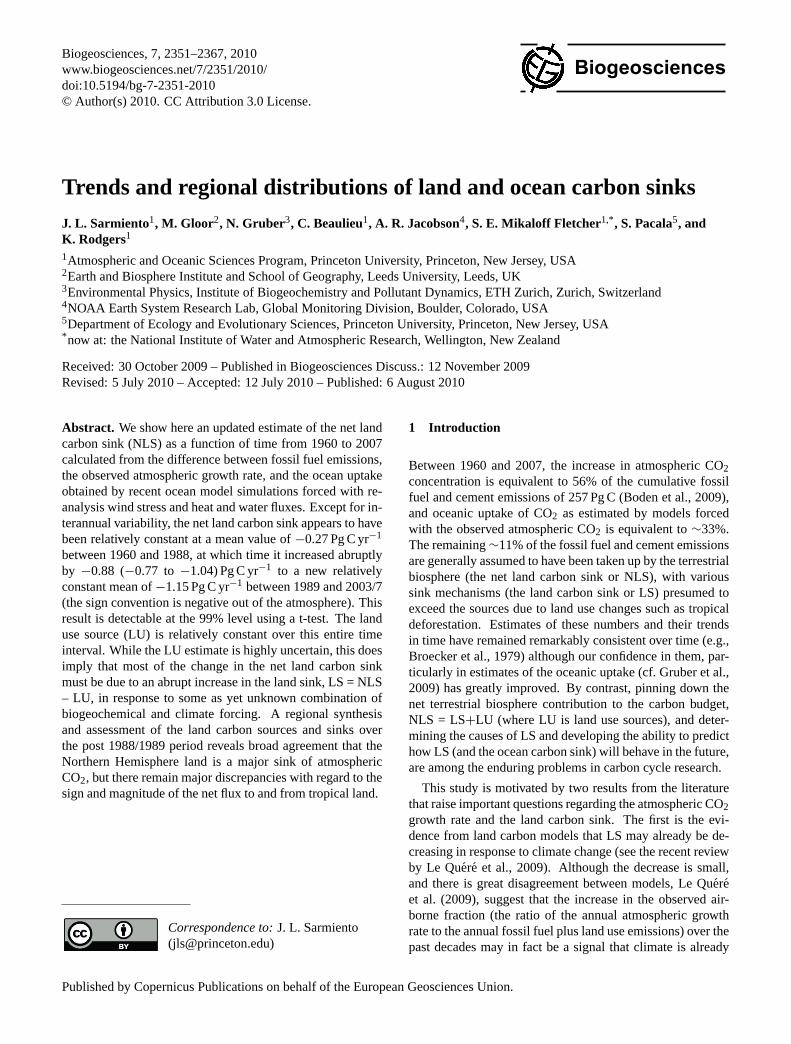
Fig. 1. Monthly deseasonalized carbon fluxes in Pg C yr−1. (a) Fossil fuel emissions and annual atmospheric growth rate calculated withMauna Loa data (see Appendix A for data sources and methods). Major volcanic eruptions and ENSO events are identified by their dates.(b) Net atmosphere-ocean fluxes of CO2 as simulated by ocean models. The solid black line labeled Mikaloff Fletcher et al. (2006) representsthe expected temporal evolution of the ocean uptake if there is no change in ocean circulation and transport. By construction, this goes throughour best data and model based estimates of ocean CO2 uptake of∼2.2±0.2 Pg C yr−1 for the 1990s and early 2000s (cf. Gruber et al., 2009).The Le Quere et al. (2007), Lovenduski et al. (2008), Rodgers et al. (2008) and Wetzel et al. (2005) results are from ocean “hindcast”simulations, where an ocean carbon cycle model is forced with re-analyzed variations of wind, and freshwater and heat fluxes over the lastfew decades. The Le Quere et al., Rodgers et al., and the Lovenduski et al. simulations all overlap the Mikaloff Fletcher et al. result duringthe 1990s. The Wetzel et al. ocean carbon sink estimate is somewhat on the low side, though its behavior in time, which is the aspect of thesemodels that we emphasize in the discussion, is similar to that of the others.(c) Net atmosphere-land fluxes of CO2 estimated by subtractingthree model estimates of the ocean sink from panel (b) and the atmospheric CO2 growth rate from panel (a) from the fossil fuel emissionsshown in panel (a). The smooth lines are from a Butterworth filter with a five year smoothing time scale.

www.biogeosciences.net/7/2351/2010/ Biogeosciences, 7, 2351–2367, 2010


volcanic eruption events, particularly during and after the Mt.Pinatubo eruption of June 1991 (Jones and Cox, 2001; Rod-erick et al., 2001; Gu et al., 2003; Peylin et al., 2005;). Theocean usually has an opposite impact on the observed atmo-spheric CO2 growth rate due to the suppression of Equato-rial CO2 outgassing during El Nino resulting from reducedupwelling of carbon, with the opposite occurring during LaNina events (Feely et al., 2006). However, this effect is muchsmaller than the land effect.

2.3 Oceanic CO2 uptake

A recent set of ocean carbon cycle models has been devel-oped with the goal of simulating the time-varying nature ofocean circulation over the last few decades by forcing withwind and heat and water fluxes from reanalysis of observedmeteorological fields (Wetzel et al., 2005; Le Quere et al.,2007, 2009; Lovenduski et al., 2008; Rodgers et al., 2008).The subset of these simulations shown in Fig. 1b suggest thatstarting in the mid to late-1980’s there was a leveling off ofoceanic CO2 uptake (Fig. 1b). This came as something ofa surprise, since previous simulations with both steady-stateocean models and coupled climate models forced with theobserved CO2 had predicted that ocean uptake should haveincreased over this time period. As an example of such mod-els, we show in Fig. 1b the results of a ten-model ocean in-version designed to estimate surface carbon fluxes consistentwith ocean interior data from the global ocean carbon surveyof the 1990s (Mikaloff Fletcher et al., 2006). As the modelsunderlying this inversion were forced with a climatic aver-age of seasonally varying winds and heat and water fluxes,the estimated surface carbon fluxes reflect a climatological-mean uptake and vary only in response to the increase in at-mospheric CO2.

As regards the location and mechanisms of the reducedoceanic CO2 uptake simulated by the models, a large portionof it occurs in the Southern Ocean, where an intensificationof winds over time leads to increased upwelling of watersrich in pre-anthropogenic dissolved inorganic carbon (DIC)that is then released to the atmosphere as CO2 (Wetzel etal., 2005; Le Quere et al., 2007; Lovenduski et al., 2007,2008). The enhanced upwelling also accelerates the uptakeof anthropogenic CO2, but this effect is smaller (Lovenduskiet al., 2008). Taken together, these changes in wind forcingreduce the Southern Ocean net sink for atmospheric CO2.Climate model simulations are able to reproduce a similarintensification of the winds resulting from a combination ofincreased greenhouse gases and stratospheric ozone deple-tion (cf. Thompson and Solomon, 2002; Chen and Held,2007; Lenton et al., 2009). Ongoing studies are analyzing thetrends in ocean model regions outside the Southern Ocean aswell as the sensitivity of ocean models to forcing with otherreanalysis products.

Time series observations of air-sea CO2 fluxes are ex-tremely limited, but there is evidence from 23 years of ob-

servations in the Equatorial Pacific of an increase in the out-gassing flux of 0.09±0.16 Pg C yr−1 after the Pacific DecadalOscillation regime shift of 1997–1998 (Feely et al., 2006).There is also evidence of a decline of 0.24±0.1 Pg C yr−1

in CO2 uptake in the North Atlantic between 20◦ N and65◦ N sometime during the period between 1994/1995 and2002–2005 (Schuster and Watson, 2007). By contrast, in theNorth Pacific, the observed rate of increase of surface oceanpCO2 over a 35 year period lags the atmospheric growth rateslightly (though the difference in growth rates is not statis-tically significant), and in the Bering Sea and periphery ofthe Sea of Okhotsk, the surface oceanpCO2 has actually de-creased over time (Takahashi et al., 2006), suggesting that inthis region the uptake may have increased over time. Fur-thermore, observations from the Hawaii Ocean Time series(HOT) and Bermuda-Atlantic Time series (BATS) stationsshow little evidence of a long-term trend in the air-sea gra-dient of CO2 (e.g. Gruber et al., 2002; Keeling et al., 2004;Bates, 2007; Dore et al., 2009). The observational analy-ses and model results thus suggest that the decline in oceanicuptake, if it stands up to continued investigation, is likely acomplex global scale phenomenon that alters the current dis-tribution of oceanic sources and sinks, and that it involveschanges in both the “natural” carbon cycle that existed be-fore the Anthropocene as well as to the rate of uptake of theanthropogenic perturbation per se.

2.4 Net land sink

Figure 1c shows our global carbon budget estimate of the an-nual net fluxes of CO2 between the atmosphere and the landbiosphere calculated by taking the difference between fossilfuel emissions and the annual atmospheric growth rate andoceanic uptake. Since these land fluxes are computed by dif-ference, it is important to have in mind that they also reflecterrors in the component sources and sinks that go into the cal-culation. Three estimates are shown based on the ocean mod-els from Fig. 1b. The estimate using the Mikaloff Fletcher etal. (2006) results are representative of the expected behav-ior of the net land flux if the ocean circulation had remainedconstant over time, while the other two estimates represent anupper (Le Quere et al., 2007) and lower (Wetzel et al., 2005)limit of the inferred increase in net land fluxes if the ocean-atmosphere CO2 fluxes change in response to time-varyingocean circulation and biogeochemistry.

The predominant signal in the inferred net land flux ofFig. 1c is the very large interannual variability. A compar-ison of Fig. 1a, b, and c shows that most of this interannualvariability carries over from the atmospheric growth rate,i.e. much of it is associated with ENSO variability. In ad-dition, it has been shown that cooler than normal episodesassociated with explosive volcanic eruptions, such as thePinatubo eruption in 1991 tend to lead to a negative net landflux, i.e., enhance the net uptake by the land (Jones and Cox,2001).



Table 1. The mean of net land uptakes for the periods 1960–1988 and 1989–2003/7 and the difference1=1989–2003/7 minus 1960–1988 using each of the ocean models shown in Fig. 1b. The net land uptake numbers are calculated from the annual means to remove theautocorrelation.

1960–1988 1989–2003/7 1 pb

Reference ocean modela−0.32 −0.96 −0.64±0.30 0.02∗

Le Quere et al. (2007) 0.04 −1.01 −1.04±0.31 0.00∗∗

Lovenduski et al. (2008) −0.45 −1.34 −0.89±0.32 0.00∗∗

Rodgers et al. (2008) −0.13 −0.90 −0.77±0.32 0.01∗∗

Wetzel et al. (2005) −0.54 −1.36 −0.83±0.34 0.01∗∗

MEAN −0.27 −1.15 −0.88

a Reference ocean model is the ocean uptake and net land uptake calculated using the constant climate ocean inverse model result of Mikaloff Fletcher et al. (2006).b p is thep-value. The null hypothesis that the 1960–1988 mean is equal to the 1989–2003/7 mean is tested against the alternative that the 1960–1988 mean is smaller than the

1989–2003/7 mean using a t-test. Thep-value is the probability, under the null hypothesis, of observing a value at least as extreme as the observed test statistic. The smaller the

p-value, the more significant the test is.∗ Significant at 5% critical level (or 95% confidence level).∗∗ Significant at 1% critical level (or 99% confidence level).

Despite the magnitude of the variability, it is possible tonote a tendency for the net land fluxes to be more negativeafter 1988/1989 than before, reflecting a stronger sink. Weshow in Fig. 2 the cumulative net land uptake estimated from1960 onwards. Cumulative distribution plots such as this area useful way of low-pass filtering observations, provided onehas in mind that the smoothing is progressively greater as onegoes from the early part of the record when the cumulativeflux is small to the latter part of the record where it becomesmuch larger. In a diagram such as this, a line with a constantslope implies a constant land flux. If the land carbon sinkwere increasing with time, as might be expected if the landuptake were due to CO2 fertilization, the cumulative land in-ventory would be concave downwards, unless the fertiliza-tion effect became saturated. This view of the data suggeststhat the net land flux varied about a relatively constant meanbefore 1988/1989, and that it varied about a higher mean af-ter 1988/1989. The climate impact of the Pinatubo eruptionled to a large increase in the net land carbon inventory be-tween 1991 and 1993, after which the cumulative land car-bon inventory settled back again, but continued to increase ata faster pace (steeper slope) than before 1988/1989. In otherwords, not only does the CO2 uptake of the Pinatubo era ap-pear to have been retained by the land, but it also appearsthat the land shifted to a higher overall uptake rate than be-fore, possibly beginning in 1988/1989, before the Pinatuboeruption.

The net land sink estimated using the four time-varyingocean models of Fig. 1b increases by an average of−0.88(−0.77 to−1.04) Pg C yr−1 (p-value = 0.00 to 0.01) from−0.27 (0.04 to−0.54) Pg C yr−1 before the 1988/1989 bendin the cumulative uptake to−1.15 (−0.90 to−1.36) there-after (see Table 1). Without the years of maximum Pinatubo

10

0

-10

-20

-30

-401960 1970 1980 1990 2000 2010

Cum

ulat

ive

Net

Lan

d Si

nk (P

g C

)

Year

using Le Quéré et al. (2007)

using Lovenduski et al. (2008)using Wetzel et al. (2005)

using Rodgers et al. (2008)

Fig. 2. Cumulative net land uptake starting from 1960 calculatedfrom the results in Fig. 1c.

impact in 1991–1993, the increase is still quite large,−0.72(−0.56 to−0.92) Pg C yr−1 (p-value = 0.00 to 0.05). Anincrease in the net land carbon sink such as we observehad been noted previously for the 1990s relative to the1980s (Schimel et al., 2001). However, our analysis sug-gests that there may have been a much greater persistencein time of this signal, including that the major Pinatuboanomaly of 1991 to 1993 can account for only−0.17 (−0.12to −0.21) Pg C yr−1 of the −0.88 Pg C yr−1 increase in ourlong-term averages.



Table 2. Mean of ocean uptakes in the ocean models in Fig. 1b for the periods 1960–1988 and 1989–2003/7 and the difference1=1989–2003/7 minus 1960–1988. Only the reference model and Le Quere et al. (2007) models were run out to 2007, The Wetzel et al. (2005) modelwas run out to 2003, and the Rodgers et al. (2008) and Lovenduski et al. (2008) models were run out to 2004 (see Appendix A). Also shown is1Model X−Reference=1989–2003/7 average minus 1960–1988 average of the year-by-year difference between each model (Model X) minusthe reference constant climate model of Mikaloff Fletcher et al. (2006). The mean ocean uptakes are calculated using the annual mean oceanuptake to remove the autocorrelation.

1960–1988 1989–2003/7 1 pb 1cModel X−Reference pb

Reference ocean modela−1.41 −2.36 −0.95±0.08 0.00∗

Le Quere et al. (2007) −1.77 −2.20 −0.44±0.07 0.00∗ 0.49±0.07 0.00∗

Lovenduski et al. (2008) −1.28 −1.80 −0.51±0.10 0.00∗ 0.34±0.09 0.00∗

Rodgers et al. (2008) −1.60 −2.16 −0.57±0.07 0.00∗ 0.26±0.05 0.00∗

Wetzel et al. (2005) −1.19 −1.70 −0.51±0.08 0.00∗ 0.32±0.08 0.00∗

MEAN −1.46 −1.97 −0.51 – 0.35 –

a Reference ocean model is the ocean uptake and net land uptake calculated using the constant climate ocean inverse model result of Mikaloff Fletcher et al. (2006).b p is thep-value. The null hypothesis that the 1960–1988 mean is equal to the 1989–2003/7 mean is tested against the alternative that the 1960–1988 mean is smaller than the

1989–2003/7 mean using a t-test. Thep-value is the probability, under the null hypothesis, of observing a value at least as extreme as the observed test statistic. The smaller the

p-value, the more significant the test is.c 1Model X−Referencediffers slightly from 1Model X−1Reference for the Lovenduski et al. (2008), Rodgers et al. (2008) and Wetzel et al. (2005) simulations because

1Model X−Referenceis calculated only over the period covered by the Model X simulations (2003 for Wetzel et al. and Rodgers et al.; 2004 for Lovenduski et al.).∗ Significant at 1% critical level (or 99% confidence level).

2.5 Uncertainties and implications of global carbonbudget analysis

We emphasize that our estimate of the net land uptake iscalculated as the difference between fossil fuel emissions,the atmospheric growth rate, and the oceanic uptake. Therequirement for an increase in the net land carbon sink of−0.88 (−0.77 to−1.04) Pg C yr−1 after∼1988/1989 arisesfrom the fact that the atmosphere and ocean in combinationare taking up a smaller portion of the fossil fuel emissionsthan they were prior to 1988/1989, which means that the landmust account for more. The range in these estimates comesjust from the range in ocean model simulations, not includ-ing uncertainties in fossil fuel emissions and the atmosphericgrowth rate. We noted earlier that the uncertainty in fossilfuel emissions is estimated as±6%, which puts it in the sameballpark as the uncertainty in the atmospheric growth rate of±0.55 Pg C yr−1. We present here the average of the fossilfuel emissions and atmospheric growth rate estimates over aperiod of 14 to 28 years. Treating each year of data as in-dependent gives an uncertainty of the mean fossil fuel emis-sions and atmospheric growth rate that is a factor of

√14 to√

28 ≈ 4 to 5 smaller than the error of the individual mea-surements, i.e.,±0.1 Pg C yr−1, which is comparable to therange obtained by the ocean models.

What can we say about the uncertainty in the ocean carbonsink and its change over time? We can estimate the reductionin the oceanic carbon sink after 1988/1989 as follows: the1989–2003/7 mean sink estimated by the constant climateocean inversion shown in Fig. 1b and Table 2 is higher by

−0.95 than the mean sink between 1960 and 1988. As Fig. 3and Table 2 show, the average increase in the oceanic sinkfor the 1989–2003/7 period versus the 1960–1988 period bythe models that are subject to time-varying forcing is only−0.51. The difference between these ocean model resultsshow that, on average, the time-varying ocean models takeup 0.35 (0.26 to 0.49) Pg C yr−1 less CO2 between 1989 and2003/7 than they would have if ocean circulation and bio-geochemistry had remained constant. The changes that weshow in Table 2 are detectable at the 99% confidence levelfor each model simulation. However, this statistical analy-sis takes into consideration only the strength of the signaland the variability as predicted by each model individuallyas compared to the Mikaloff Fletcher et al. (2006) ocean in-version. Other potential sources of error include:

1. The use of different ocean circulation and biogeochemi-cal models. The range in our four model results, 0.26 to0.49 Pg C yr−1, gives some idea of how large this sourceof uncertainty is likely to be.

2. The baseline constant climate scenario. A more appro-priate way to simulate the baseline constant climate sce-nario would be to do this separately for each model.This has now been done for a set of 4 models as summa-rized by Le Quere et al. (2009) and the post-1988/1989minus pre-1988/1989 difference that we calculate fromthe average of their 4 models is 0.26±0.05 Pg C yr−1 de-tectable at the 99% confidence level. This is within therange of our estimates.



6.93±0.19

-3.60±0.28

(-1.7 to -2.2)

(-0.9 to -1.4)

1989

-200

3/7

1989

-200

3/7

4.37±0.20

-2.64±0.22(-1.2 to -1.8)

(-0.0 to -0.5)

Fossil Fuel Emissions

Atmospheric Increase Ocean Uptake Net land flux19

60-1

988

1960

-198

8

1.3±0.8

-0.5±0.3 -0.5±0.3

Tropicaldeforestation

-1.4±0.8

Tropicaluptake

N. Americatemperate

uptake

Eurasiantemperate

uptake

GLOBAL FLUXES BREAKDOWN OF LAND FLUXESFOR POST 1988/89

-5

-3

-1

1

3

5

7

-4

-2

0

2

4

6

Car

bon

Flu

xes

(Pg

C y

r-1)

-2.0

-1.2-1.5

-0.3

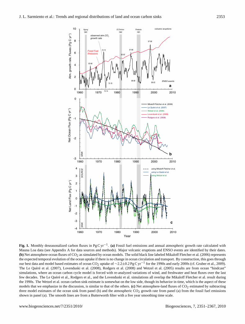
Fig. 3. Global flux estimates for 1960 to 1988 and 1989 to 2003/7 obtained by averaging the fluxes shown in Fig. 1 and Table 2. The shadedregion on the right summarizes the post-1988/1989 bottom-up land source and sink components discussed in the text.

3. Sensitivity to the reanalysis product used to force theocean models and whether the atmospheric forcingfields represent skillfully decadal variations in the stateof the atmosphere. The Le Quere et al. (2009) supple-mentary material shows a series of ocean model sim-ulations with different reanalysis products that appearto indicate only minor differences, but this issue needsfurther examination.

4. Whether the models are simulating oceanic variabilitycorrectly. While observational constraints on this arelimited, there are some observations discussed above;and model studies such as those referenced earlier(cf. also Doney et al., 2009) tend to show that modelsoverall do a reasonable job of simulating observed vari-ability.

5. Whether the models have all the correct physical pro-cesses. In particular additional model studies are neededto examine the extent to which eddy transfer in theocean may in fact cancel some of the effects of in-creased wind-driven Ekman divergence in the SouthernOcean (cf. Hallberg and Gnanadesikan, 2006; Boninget al., 2008). It is currently an area of active research todetermine whether the mesoscale parameterization usedin the global models represented in Fig. 1b is adequateto represent the effect of eddy transfer found in higherresolution models.

Our analysis suggests that the oceanic carbon uptake laggedthe growth that would have been expected if ocean circula-tion and biogeochemistry had remained constant by about0.35 (0.26 to 0.49) Pg C yr−1 after 1988/1989. Summing ourestimated reduction in oceanic uptake to the increase in netland uptake of−0.88 (−0.77 to−1.04) Pg C yr−1 gives an

estimated reduction in the atmospheric growth rate of−0.53(−0.51 to−0.55) Pg C yr−1. The uncertainty in these esti-mates is large, particularly when one considers the additionaluncertainty of order±0.1 Pg C yr−1 contributed by the fossilfuel emissions and atmospheric growth rate. However, if theyhold up to further scrutiny, the implications for the land car-bon sink are dramatic given that they represent more than aquadrupling of the net land carbon sink and a 50% increase inthe absolute magnitude of the total annual land carbon sinksince 1960 (see discussion in Sect. 4). The implied reduc-tion in atmospheric growth rate would be a challenge to de-tect, because it is relatively small compared to the observedgrowth rate and its interannual variability.

How consistent is this ocean model-based partitioning be-tween the land and ocean with other, independent constraints,such as those based on measurements of carbon-13 in theocean and atmosphere or of the atmospheric O2/N2 ratio(e.g. Battle et al., 2000; Bender et al., 2005; Manning andKeeling, 2006)? Given the uncertainties in our knowledge ofcarbon isotope fractionations and the small magnitude of thechange in the net land carbon sink relative to the interannualvariability, it is unlikely that the signal resulting from such achange in the land carbon sink could be detected in carbonisotope measurements. The O2/N2 tracer is more promising,but measurements were not initiated until after the changein the net land carbon sink occurred and the uncertaintiesin the land uptake estimates based on this tracer are verylarge. Our post-1988/1989 net land uptake estimate of−1.15(−0.90 to−1.36) Pg C yr−1 is consistent within uncertainty,though at the upper limit of the atmospheric oxygen basedestimate of−0.51±0.74 Pg C yr−1 obtained for the period of1993 to 2003 by Manning and Keeling (2006). A possibleimplication of our result is that Manning and Keeling mayhave overestimated the magnitude of the correction for the



outgassing of oxygen due to warming of the ocean. Withoutthis degassing, their estimate of the land carbon sink wouldbe−0.99 Pg C yr−1.

3 Regional land carbon flux distribution after1988/1989

We turn now to a discussion of the regional distribution ofthe land carbon source and sink components to examine theirconsistency with our global carbon budget estimates of thenet carbon flux and see what clues such estimates may offeras to the cause of the acceleration in the net terrestrial uptakeand its spatial distribution (see gray area in Fig. 3). We beginwith bottom-up estimates based on in situ measurements andmodels, then proceed to a discussion of top-down estimatesbased on inverse models.

3.1 Bottom-up estimates

The main terrestrial source of CO2 to the atmosphere is trop-ical land use change (mainly deforestation), which has var-iously been estimated as either∼1.1±0.3 Pg C yr−1 basedon analyses of satellite observations (Achard et al., 2002,2004; DeFries et al., 2002) for the 1980s and 1990s, or∼2.2±0.6 Pg C yr−1 from “bookkeeping” methods based onFAO expert opinion and official governmental estimates fromthe 1990s (Houghton, 2003; cf., Food and Agriculture Or-ganization, 2001; Fearnside, 2000). (Bookkeeping methodstrack the amount of carbon released to the atmosphere fromclearing and decay of plant material, plus the amount of car-bon accumulated as vegetation grows back.) However, morerecently, Houghton (2007) revised his bookkeeping estimatesdown to ∼1.5±0.8 Pg C yr−1 for the period between 1960and 2006. This includes an estimate of non-tropical landuse change, but the non-tropical component is<4% after1988/1989. The reduction in uptake is due primarily to re-vised FAO tropical land use change estimates (R. Houghton,personal communication, 2009; note, however, that the re-liability of FAO inventories is unclear; Grainger, 2008). Inaddition, there are some new estimates by Shevliakova etal. (2009) that combine the bookkeeping and satellite meth-ods, giving estimates that are as low as 1.1 Pg C yr−1 overthis time interval. In what follows, we will use for our es-timate of the tropical land use change source the medianof these new estimates, 1.3 Pg C yr−1 with a nominal uncer-tainty of±0.8 Pg C yr−1.

Bottom-up estimates of land carbon sinks are only avail-able for the post-1988/1989 period. The most complete in-ventory of land carbon sinks is for North America for circa2003 (Pacala et al., 2007). This shows a net carbon sinkof −0.5±0.3 Pg C yr−1 with ∼60% from the forest sectordue to increases in the mean age of forest stands becauseof relaxed rates of harvest, agricultural abandonment, andfire suppression. The remaining sink is due to other hu-

man activities such as construction of dams, the practicesof the forest products and waste disposal industries, and ac-cumulation of carbon in wood products and landfills, reser-voirs, pasture lands and wetlands. Research is mixed onthe role that fertilization by nitrogen or CO2 plays in theNorth American carbon sink (Pacala et al., 2007). Inven-tories from Eurasia are less complete, but by augmenting theestimates for the temperate and boreal Eurasian forest sector(−0.3±0.1; Goodale et al., 2002) with the non-forest sec-tor implied by the North American inventory, we arrive atan estimate of−1.0±0.5 Pg C yr−1 for the combined northtemperate and boreal zones. Both this estimate and its uncer-tainty must be viewed as tentative. Although estimates fromeddy-covariance studies have provided useful local confirma-tion of the inventory methods (Barford et al., 2001; Pacalaet al., 2007), they cannot be used yet to determine averagefluxes over large regions (though see Jung et al., 2009). Thisis because the network of such sites is too small to averageaccurately over heterogeneity in the physical environmentand terrestrial land use, and there continue to be concernsof bias due to the inability to retrieve fluxes during periodsof stratification, which occur primarily at night when ecosys-tems are a net source of CO2.

Carbon inventory measurements in mature tropical forestsare far less extensive than temperate inventory estimates.Measurements of a 60 000-tree network across Amazonia in-dicates that primary forest gained carbon during the 1990’sat an average rate of−0.8±0.3 Pg C yr−1 (Phillips et al.,2009). Using similar data from fewer but much larger plotsfrom Southeast Asia (6 plots) and Africa (2 plots) (Chaveet al., 2008) and the same reasoning as in the Amazonianstudy by Phillips et al. (1998) to extrapolate these studiesspatially, we obtain a total tropical mature forest sink esti-mate of−1.4±0.8 Pg C yr−1. This number is consistent withthe just published study of Lewis et al. (2009) which reportsresults from 79 plots of∼1 ha area in Africa, which werecombined with growth trends estimated from South Amer-ican and Asian tropical plots, to obtain a pantropical sinkestimate in old-growth forests of−1.3 Pg C yr−1 (confidenceinterval =−0.8 to−1.6) over the last decades. Whether ornot these measurements are sufficiently broad in scope to berepresentative is being hotly debated in the literature, as is themechanism (e.g., Malhi et al., 2008). Some have suggestedthat the pantropical sink is due to growth stimulation in re-sponse to a changing environment including elevated CO2,changes in temperature and precipitation, modified insola-tion or diffuse radiation; while others have argued that it israther a response to a changing disturbance regime or pos-sibly recovery from a large scale mega-disturbance event oreven simply a measurement artifact.

Summing up our bottom-up estimates of the north tem-perate and boreal terrestrial carbon sinks together with ourestimate of the tropical sink, we arrive at a global terres-trial carbon sink estimate of−2.4±0.9 Pg C yr−1 for thepost-1988/1989 period. Given our tropical land use source



TROPICAL AND SOUTHERN HEMISPHERE LAND

−3

−2

−1

0

1

2

NORTHERN HEMISPHEREEXTRATROPICAL LAND

SOUTHERN OCEAN TROPICAL OCEAN NORTHERN HEMISPHEREEXTRATROPICAL OCEAN

Ocean (pCO2 -based)

Atmosphere InverseAtmosphere Inverse Stephens SubsetJoint Inverse Joint Inverse Stephens Subset

Land (Inventory & deforestation-based)

−1

0

1

2

SOUTHERN HEMISPHERETEMPERATE OCEAN

BOTTOM-UP ESTIMATES

TOP DOWN ESTIMATES

CO

2 Flu

xes

(Pg

C y

r-1)

CO

2 Flu

xes

(Pg

C y

r-1)

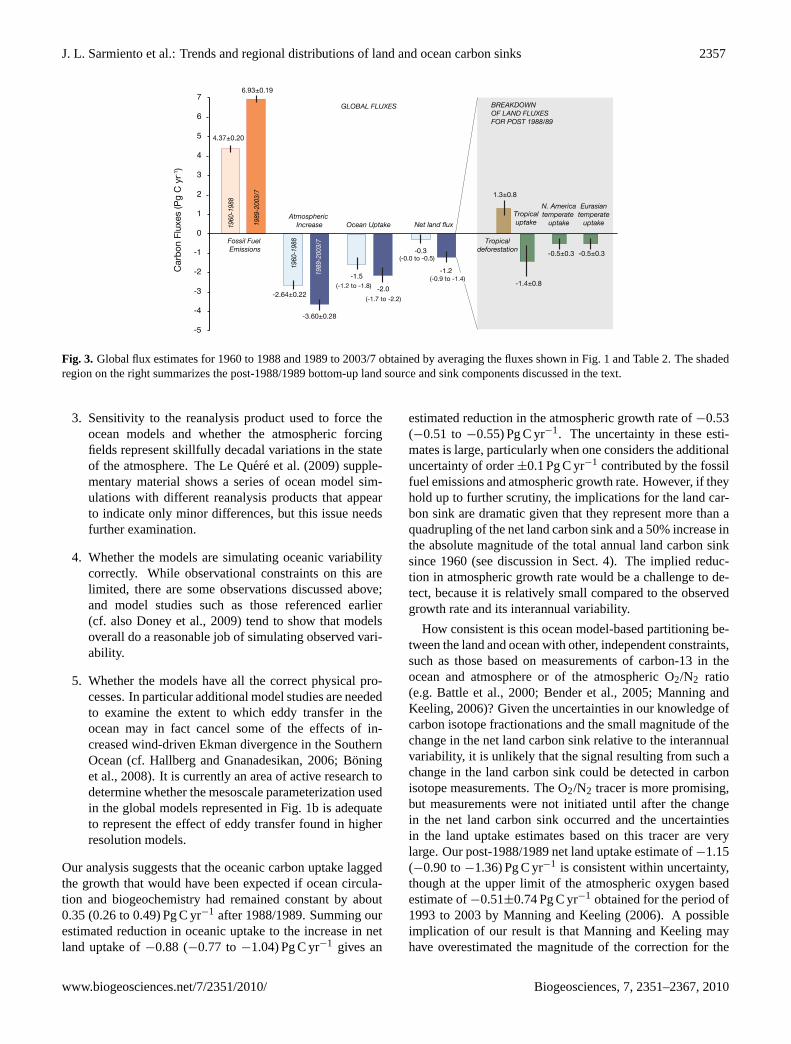
Fig. 4. Regional flux estimates for the land and ocean. The bottom-up land inventory estimates are as described in the text and shown inFig. 3. The oceanpCO2 based estimates are from Takahashi et al. (2009), the atmosphere inverse results are from the Transcom-3 studyof Gurney et al. (2004), the “Atmosphere Inverse Stephens Subset” is from a new atmospheric inverse calculation we did as part of thisstudy using a subset of three of the Transcom-3 atmospheric transport models that provide a better fit to certain criteria based on observedvertical profiles of CO2 in the atmosphere (Stephens et al., 2007), the joint inverse is from Jacobson et al. (2007a), and the “Joint InverseStephens Subset” is from a new calculation we did using the Stephens subset of Transcom-3 models. Note that the oceanic data constrain theair-sea flux so strongly that the results of ocean-only inverse studies (e.g., Gruber et al., 2009), i.e., those that do not include the atmosphericconstraint used in the joint inverse, give virtually the same answer as the joint inverse. The latitude boundaries used to calculate the oceanuptake are 44◦ S, 18◦ S and 18◦ N.

estimate of 1.3±0.8 Pg C yr−1, we obtain a total bottom-upnet land sink estimate of approximately−1.1±1.2 Pg C yr−1.This is in very good agreement with our global carbon bud-get post-1988/1989 net land sink estimate of−1.15 (−0.90to −1.36) Pg C yr−1 (Table 1 and Fig. 3). These bottom-upestimates of the land carbon sinks and land-use changesources also provide a picture of the regional distributionof carbon sources and sinks, with an estimated net sink of−1.0±0.5 Pg C yr−1 in the temperate and boreal NorthernHemisphere and a tiny net sink of−0.1±1.1 Pg C yr−1 in thetropics (uptake of−1.4±0.8 Pg C yr−1 minus land use sourceof 1.3±0.8 Pg C yr−1).

We note that while the global carbon budget estimate ofFig. 1c shows that interannual variability of the net land car-bon sink is very large (±3 Pg C yr−1), the measurements un-derlying the bottom-up estimates mostly span a long periodof time so that the appropriate global carbon budget estimateto compare them with is the long-term average, as we havedone (see Fig. 4).

3.2 Top-down estimates

Another method to estimate the regional distribution of car-bon sources and sinks is the top-down atmospheric inversionmethod, where a set of regionally resolved ocean-atmosphereand land-atmosphere carbon fluxes are adjusted to be opti-mally consistent with the observed atmospheric CO2 distri-bution. One of the most prominent of such studies is theTranscom-3 inversion intercomparison, which used average

data for the period between 1992 and 1996 (Gurney et al.,2004; cf. Denman et al., 2007). While this period includesthe tail end of the Pinatubo anomaly, the average net landcarbon sink over the period is similar to that over the entireperiod from 1988/1989 to 2007 (cf. Fig. 1c). The Transcom-3 inversions obtained a net source of carbon in the tropicaland Southern Hemisphere land and a large net sink for car-bon in the Northern Hemisphere land (orange bars in Fig. 4).

The uncertainties in the Transcom-3 atmospheric in-verse land uptake estimates and the bottom-up land up-take estimates overlap, but there is a rather large offsetof ∼1 Pg C yr−1 between them, with the atmospheric in-verse showing a large tropical source where the bottom-upestimates show a near zero flux and the atmospheric in-verse showing a much larger sink in the extratropics thanthe bottom-up estimates. Furthermore, there is a large dis-crepancy between the air-sea flux estimates obtained by theTranscom-3 atmospheric inversions and independent air-seaflux estimates obtained both by air-seapCO2 difference mea-surements combined with a gas exchange model (blue barsin Fig. 4; Takahashi et al., 2009), and by ocean inverse es-timates (light green bars; Gruber et al., 2009). The dis-agreement is particularly striking in the tropical ocean, wherethe Transcom-3 atmospheric inverse models tend to underes-timate the degassing flux relative to the ocean observationbased estimates; in the Southern Hemisphere temperate lat-itudes, where atmospheric inverse models tend to underesti-mate the uptake relative to the observation based estimates;



and in the Southern Ocean, where the atmospheric inversemodels tend to overestimate the oceanic sink relative to theobservation based estimates (cf. Gruber et al., 2009).

The use of ocean interior constraints on air-sea fluxes ina joint atmosphere-ocean inversion ensures that the solutionobtained is consistent with the air-sea flux estimates of Ja-cobson et al. (2007b). However, the land carbon flux solu-tion obtained in this way (light green bar in the upper part ofFig. 4) differs from the terrestrial bottom-up estimates by al-most 2 Pg C yr−1, with the joint inverse giving a much largersource in the tropics and Southern Hemisphere, and a muchlarger sink in the northern extra tropics than the bottom-upestimates. These are large differences, but unfortunately theuncertainties on the terrestrial flux estimates are so large thatthe differences are statistically significant at the one standarddeviation level only for the Northern Hemisphere extratrop-ics.

An important source of error in atmospheric inversions isthe uncertainty in atmospheric transport, which needs to bespecified from an atmospheric transport model in order todetermine how atmospheric CO2 changes at a particular lo-cation in response to fluxes at the surface. The uncertainty inthis transport is difficult to quantify and is usually assessedby model intercomparison, as in the Transcom-3 study. Ina recent study that made use of new vertical CO2 profilesin the atmosphere (Stephens et al., 2007), only three of theTranscom-3 atmospheric transport models were found to beconsistent with the annual mean observed vertical gradientsof CO2 in the annual mean (though this was due to a cancel-lation of errors in the seasonal profiles). However, while thissubset of models did change the land fluxes somewhat, in factbringing them into better agreement with the bottom-up landflux estimates, they compare poorly with the ocean-basedflux estimates (Fig. 4). Using these three atmospheric trans-port models in the joint inverse gives results shown in thedark green bars in Fig. 4 that are similar to the full Transcom-3 model suite for air-sea fluxes, with slight changes on landtending to give fluxes that are in slightly better agreementwith the bottom-up estimates.

Solving the inconsistencies between the bottom-up andtop-down estimates of the regional distribution of landsources and sinks for atmospheric CO2 has to comprise allfour of the following: (1) improved bottom-up land carbonflux estimates including particularly carbon inventory mea-surements with improved measurements of soil carbon in-ventory; (2) incorporating the new oceanic constraints intoatmospheric analyses and exploring the extent to which it ispossible to fit both these and the bottom-up land flux esti-mates simultaneously; (3) improved atmospheric transportmodels; and (4) improved atmospheric observational con-straints, of which vertical profiles and the possibility of ob-taining atmospheric CO2 data from satellite observations aresignificant developments.

4 Discussion and conclusions

We have examined the atmospheric growth rate (AGR),oceanic uptake (OS), and net land carbon sink (NLS), thesum of which is required to equal the fossil fuel emissions(i.e., FF = AGR + OS + NLS). Observational and modelbased estimates enable us to determine three of these fourvariables with reasonable confidence, namely AGR, OS, andFF, from which we are able to estimate the fourth, NLS. Asregards the ocean carbon sink, our comparison of the oceanuptake in four models with reanalysis climate forcing versusmodels with constant climate forcing led to the conclusionthat oceanic uptake may have slowed relative to expectation,in agreement with previous studies (Canadell et al., 2007; LeQuere et al., 2007; Lovenduski et al., 2007; cf. Le Quere etal., 2009).

As regards the net land carbon sink NLS, our analysisshows that it appears to have been small between 1960 un-til ∼1988/1989 (Figs. 1c and 3), with the longer-term recordshown in Fig. 5 suggesting that it may have been at or nearzero (the cumulative flux was nearly constant) from as earlyas ∼1930. The net land carbon sink appears to have in-creased after 1988/1989. The nature of the increase is ex-tremely difficult to detect given the short time scale of therecord, the huge variability of the net land uptake estimate,and the differences between the land uptake estimates ob-tained with the different ocean models. Thus it is difficult forus to say whether the increase represents an abrupt shift to ahigher uptake or a more gradual increase, though the cumu-lative NLS in Fig. 2 and LS in Fig. 6b suggest an abrupt shiftis more likely.

What might have caused the net land carbon sink to in-crease after 1988/1989? The net land carbon sink NLS, isequal to the difference between the land sink LS and the landuse source LU, i.e., with the sign convention being negativefor removal from the atmosphere, NLS = LS + LU. Thus,an increase in the absolute magnitude of NLS could havebeen caused either by an increase in the absolute magnitudeof the land sink LS or a decrease in the magnitude of theland use LU or some combination of these. Up to now wehave avoided separating the time history of the net land car-bon sink into its components because of the low confidencelevel in the land use estimates. However, as Fig. 6a shows,the land use source LU as presented in Houghton (2007) andCanadell et al. (2007) has, if anything, increased slightly intime, which implies that the increase in the absolute magni-tude of the net land carbon sink NLS must be due primarilyto an increase in the absolute magnitude of the land carbonsink LS (Figs. 5c and 6a and b). The only estimates of LUdiscussed in the review by Le Quere et al. (2009) that extendbeyond our change point of 1988/1989 are the Shevliakovaet al. (2009) and Houghton estimates, and neither of theseshows a significant drop in the sources at anywhere near1989, in agreement with Houghton (2007). The McGuireet al. (2001) and Van Minnen et al. (2009) results show a



1960 1970 1980 1990 2000 2010310

330

350

370

390

Atm

osph

eric

Car

bon

Dio

xide

(pp

mv)

260

280

300

320

340

360

380

400

1000 1200 1400 1600 1800 2000

Atm

osph

eric

Car

bon

Dio

xide

(pp

mv)

a

MAUNA LOA OBSERVATORY

Ice core&firn measurements

Atm

osph

eric

m

easu

rem

ents

-400

-300

-200

-100

0

100

200

300

400

1750 1800 1850 1900 1950 2000

Cum

ulat

ive

Flux

es (P

g C

)

Net land flux

Atmosphere

Ocean sink

Fossil fuelemissions

SOURCES

b

SINKS

200

-150

-100

-50

0

50

100

150

1750 1800 1850 1900 1950 2000

Net land flux

Land-use change source

Residual land flux

Scenario B:

Scenario B:

Cum

ulat

ive

Land

Flu

xes

(Pg

C)

SOURCES

SINKS

c

Figure 1

Scenario A:

Scenario A:

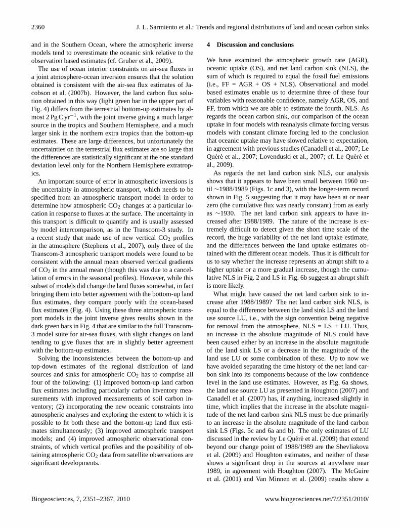
Fig. 5. Atmospheric CO2 and the cumulative carbon budget starting from 1750. Sources for data are as described in Appendix A withadditional sources given in the caption.(a) Atmospheric CO2 variations over the last 1000 years. The data until 1958 stem from a seriesof Antarctic ice cores (Barnola, 1999), while the data from 1958 onward are from the Mauna Loa Observatory in Hawaii. The inset showsthe monthly Mauna Loa measurements, whereas the main plot depicts the annual means.(b) Cumulative carbon fluxes from 1750 onwardsof the main sources and sinks of the global carbon cycle including fossil fuel emissions, the atmospheric CO2 increase, ocean uptake, andnet land flux. The atmospheric increase is calculated from a spline fit to the ice core and Mauna Loa CO2 data from (a), the ocean uptakeis based on the ocean inversion of Mikaloff Fletcher et al. (2006) scaled to the respective year assuming a linear relationship between oceanuptake and atmospheric CO2 (see Appendix A) and the net land flux is computed by the difference Net land flux = fossil fuel emissions –atmospheric CO2 increase – ocean uptake. The symbols are estimates from Sabine et al. (2004) for the period from 1800 to 1994 summedto the 1790 to 1810 average of our estimates.(c) The cumulative net land flux from panel (b) (solid blue line) plus two additional scenariosfor the net land flux based on the oceanic uptake estimates of Le Quere et al. (2007; Scenario A) and Wetzel et al. (2005; Scenario B) whichrepresent upper and lower limits of the ocean uptake estimates from Fig. 1b, respectively. Also shown in the figure is the cumulative landuse source of Houghton (2007) for the period 1850 to 2005, which is summed in this figure to the 1850 net land flux. The total area underthis curve including the vertically hatched green area and the solid light green area is our best estimate of the total land use change sourcesof CO2 to the atmosphere. The solid green area is that portion of the source that can be accounted for by the carbon budget in panel (b). Thevertically hatched area thus must be balanced by the additional sinks shown in the lower part of this diagram.



0

-20

-40

-60

-80

-1001960 1970 1980 1990 2000 2010

Cum

ulat

ive

Land

Sin

k (P

g C

)

Year

using Le Quéré et al. (2007)

using Lovenduski et al. (2008)using Wetzel et al. (2005)

using Rodgers et al. (2008)

b

using Le Quéré et al. using Wetzel et al.

using Mikaloff-Fletcher et al.

Land Use Change Source

Land Carbon Sink

a

-4

-3

-2

-1

0

1

2

1960 1970 1980 1990 2000 2010Year

Lan

d Fl

ux (P

g C

yr-1

)

SO

UR

CE

SIN

K-5

-6

Fig. 6. (a)The annual land use change source of Houghton (2007)and the annual land carbon sink calculated as in Fig. 5 and shownfrom 1960 onwards.(b) The cumulative land carbon sink. Theannual land carbon sink also shows smoothed lines filtered with a5 year Butterworth filter. The straight lines in (b) are drawn in byhand to provide a guide to the eye showing that the slope increasesafter 1988/1989.

decrease in the land carbon sink starting ten years earlieraround 1980, but the estimates end in∼1992, too early tobe of use for this analysis.

What can observations and/or models tell us about the na-ture of the terrestrial carbon sink LS and the causes of itschanges? The bottom-up carbon sink estimates of the land-atmosphere carbon fluxes for the post-1988/1989 period sup-port the results obtained by our global carbon budget esti-mate. A next step would be to determine if such changescan be simulated in land models that are forced with landuse changes as well as reanalysis climate; and to determineif there are bottom-up observations that can tell us what wasdifferent prior to 1988/1989 and where and how the transitionto a higher land uptake occurred. There are in fact severalland model simulations that have been forced with reanaly-sis climate, though not including land use change (cf. Sitchet al., 2008). The average of five such simulations summa-rized by Le Quere et al. (2009) has a similar cumulative landcarbon sink as our data based estimates. However, this is

presumably because the models have been tuned to fit suchestimates. The land models also show a big jump in the landcarbon sink, but the timing of the jump is inconsistent withours, occurring more than a decade earlier in the mid-1970s.Moreover, the jump is attributed by Le Quere et al. (2009)to a model error due to the overestimation of the land carbonsink response to the cool/wet La Nina-like climate conditionsin the mid 1970s.

Candidates for what could be responsible for an increasein the net land carbon sink that we find include:

1. An error in the calculation of net land use due to anunderestimate of pre-1988/1989 fossil fuel emissionsor an overestimate of post 1988/1989 fossil fuel emis-sions or an error in the ocean carbon sink. The re-cent revisions to the fossil fuel estimates that we usein our calculations (cf. Boden et al., 2009) lowered thefossil fuel emissions by∼0.2 Pg C yr−1 after 2004 and∼0.1 Pg C yr−1 after 1993, which reduced our estimateof the increase in the land flux. Furthermore, the lev-eling off of the oceanic carbon sink that we showed inFig. 1b is estimated directly from ocean model simu-lations forced with reanalyzed meteorological observa-tions, and supported by a modest number of observa-tions, all of which have uncertainties as discussed inSect. 2.3. If, for example, the post-1988/1989 levelingof ocean uptake were shown to be wrong, this would re-duce our estimate of the change in the land carbon sinkfrom −0.88 to−0.64 Pg C yr−1 with p=0.02.

2. A decrease in land use emissions, which is not sup-ported by existing publications, as we have shown inFig. 6.

3. A change in the land carbon sink LS due to (a) afertilization effect such as the cumulative impact ofCO2 fertilization (cf. Schimel et al., 2004); (b) growthstimulation by climate variability such as the AtlanticMultidecadal Oscillation shift in 1996 and/or the Pa-cific Decadal Oscillation shift in 1998, both of whichcome at an opportune time following the June 1991Pinatubo eruption; (c) climate change such as the im-pact of the increased incidence of droughts after themid-1980s (Trenberth et al., 2007; Buermann et al.,2007); (d) changes in solar irradiance reaching theEarth’s surface, which began to increase about 20 yearsago after undergoing a long period of dimming due tothe impact of aerosols (Romanou et al., 2007; Weilickiet al., 2002; Trenberth et al., 2002); or (e) an increase inthe growing season length due to global warming (e.g.,Keeling et al., 1996).

We note that the net land carbon uptake NLS shown in Fig. 1cand the land carbon sink LS shown in Fig. 6a are highly vari-able in time. With such a short record, it is difficult to knowif the increase in the land uptake is due to a change in the



baseline behavior, or if it may in fact be related to changesin the variability resulting from known nonlinearities in theresponse of the hydrological cycle to ENSO variability inconjunction with nonlinearities in the terrestrial carbon re-sponse to variations in hydrological or other climate forcing.

We conclude that the net land carbon sink NLS appears tohave increased abruptly around 1988/1989 due primarily toan increase in the land carbon sink LS. We also confirm asmall reduction in the oceanic sink in models forced with re-analysis climate versus those forced with a constant climate.The difference between the increased land carbon sink andreduced ocean sink is small and uncertain, but the increasein the land uptake is larger than the reduction in the oceanuptake, implying that the atmospheric growth rate decreasedover time with respect to what would have happened if theland carbon sink had continued at its pre-1988/1989 magni-tude and the ocean had not changed in response to climate.Our analysis suggests that fundamental changes in the car-bon cycle may be underway in both the oceans and terrestrialbiosphere that pose important challenges to our mechanis-tic understanding of controls on carbon flux variability andtrends.

Appendix A

Data sources and methods

A1 Fossil fuel emissions

Annual fossil fuel emissions from 1750 through 2006 arefrom Boden et al., 2009 supplemented by Marland (personalcommunication, 2009), who provided slightly updated 2006emissions and estimates of the 2007 and 2008 emissions.These annual data were used directly in the analysis shownin Tables 1 and 2 as well as Figs. 2 and 5. The monthly datashown in Fig. 1a and used in producing Figs. 3 and 6 wereinterpolated from the annual data using the mass conservingmethod of Rasmussen (1991). We calculate the long-termaverage annual growth rate of emissions over a time inter-val from t=0 to t=T following the annual mortality conceptused in the ecological literature (Sheil et al., 1995). The al-gebraic formulation for the long-term average annual growthrate approach is

FF(T ) =FF(0) · (1 + growth rate)T

where FF is fossil fuel emissions for a given yeart . Invertingthe above equation gives the growth rate as

growth rate=

(FF(T )

FF(0)

) 1T

− 1

A2 Atmospheric growth rate

The monthly atmospheric CO2 data are obtained from thefilled data set given in column 9 ofhttp://scrippsco2.ucsd.

edu/data/insitu co2/monthlymlo.csv(Keeling et al., 2001).The annual growth rate of CO2 in Pg C shown in Fig. 1a iscalculated month by month for timet in months using theequation

dCO2

dt= γ ·[pCO2(t + 6) − pCO2(t − 6)]

γ = 2.1276Pg C

ppm

wherepCO2 is the atmospheric partial pressure of CO2 inppm. The growth rate is then smoothed with a 3-monthsboxcar filter to remove short time scale variability. The con-version factorγ is calculated as follows: atmospheric carbondioxide is reported as the dry air molar mixing ratio in ppmunits per year. This is converted to Pg C of CO2 in the atmo-sphere using the relationships:

Nair =matm

µair

µair=0.0289644+0.012011·(χCO2−0.0004

)NCO2 = χCO2 · Nair

mCO2 = µC · NCO2

whereNair is the number of moles in the atmosphere,matmis the total dry mass of the atmosphere for which we usethe estimate of 5.1352±0.0003×1018 kg from Trenberth andSmith (2005), µair is the molar mass of air in kg mol−1 forwhich we use the relationship given by Khelifa et al. (2007),χCO2 is the dry air molar mixing ratio of carbon dioxideobtained by measurements, and µC=12 g mol−1 is the mo-lar mass of carbon. The conversion factor we obtain is2.12760 Pg C per ppm of dry air in January 1960, decreasingto 2.12754 by December of 2008. We thus use a conversionfactorγ of 2.1276 Pg C per ppm of dry air.

The annual atmospheric CO2 growth rate used in Tables 1and 2 and Figs. 2 and 5 is calculated by taking the differencebetween the December and January mean at the end of theyear minus the December and January mean at the start ofthe year multiplied by the conversion factorγ .

A3 Ocean uptake

The Le Quere et al. (2007), Lovenduski et al. (2008),Rodgers et al. (2008) and Wetzel et al. (2005) monthly up-take results are from “hindcast” simulations using the dailymean (except Lovenduski et al., who use 6-h mean) NCEP-1 Kalnay et al. (1996) reanalysis winds, and freshwater andheat fluxes as described in each of the papers. All models in-clude seasonality. Annual means used in the Tables 1 and 2and Fig. 3 calculations are obtained by taking the average ofthe monthly results. The monthly ocean uptake results shownin Fig. 1b and used for the net land uptakes in Fig. 1c havebeen deseasonalized and smoothed with a 3 month boxcar fil-ter using the same approach as with the atmospheric growthrate.


http://scrippsco2.ucsd.edu/data/in_situ_co2/monthly_mlo.csv

http://scrippsco2.ucsd.edu/data/in_situ_co2/monthly_mlo.csv


The Mikaloff Fletcher et al. (2006) ocean uptake is esti-mated using their equation

OS= −2.15 ·pCO2 − 277.9514 ppm

359.6619 ppm− 277.9514 ppmPg C yr−1

wherepCO2 is the atmospheric CO2 in ppm of dry air. Theannual oceanic uptake is calculated using the annual averageatmospheric Mauna LoapCO2, and the monthly uptake isestimated using the deseasonalized and smoothed monthlyMauna Loa atmosphericpCO2 data.

Only the Le Quere et al. (2007) model has been run out tothe full length of time of our analysis in 2007. The Wetzelet al. (2005) and Rodgers et al. (2008) simulations were runout to 2003, and the Lovenduski et al. (2008) simulation wasrun out to 2004. Because the oceanic uptake is relatively flatafter 1990, the post-1988/1989 ocean uptake averages givenin Table 2 are relatively insensitive to the averaging intervalused. We present the average of all models until the mostrecent full year of each simulation, which varies from 2003to 2007.

None of the ocean or net land uptake calculations shown inthis paper include the weathering and river flux contributionof ∼0.45 Pg C yr−1, which should be subtracted from the netland uptake (thereby increasing the land uptake) and addedto the ocean uptake (thereby decreasing the ocean uptake) forcomparison with observations (cf. Jacobson et al., 2007a)

Acknowledgements.We thank G. Marland for providing his mostrecent estimates of fossil fuel emission and J. Simeon for help ondata analysis. We greatly appreciate helpful comments receivedon very early versions of this manuscript from Oliver Phillips aswell as M. Bender, R. Keeling, C. Le Quere, B. Mignone, M.Oppenheimer, D. Sigman, and R. Wanninkhof. The work of JLS onthe global carbon cycle has been supported by the Department ofEnergy under a NICCR proposal, by the NOAA Geophysical FluidDynamics Laboratory and Earth System Research Laboratory,which also supported SMF, and the Carbon Mitigation Initiativewith support from the Ford Motor Company and by BP, whichalso supported SP and KR. MG was supported by the EBI andEEE institutes at the University of Leeds, and NG by ETH Zurich.CB was supported by the Fonds Quebecois de la recherche surla nature et les technologies and by the Carbon Mitigation Initiative.

Edited by: J. Middelburg

References

Achard, F., Eva, H. D., Stibig, H.-J., Mayaux, P., Gallego, J.,Richards, T., and Malingreau, J.-P.: Determination of deforesta-tion rates of the World’s humid tropical forests, Science, 297,999–1002, 2002.

Achard, F., Eva, H. D., Mayaux, P., Stibig, H.-J., and Belward,A.: Improved estimates of net carbon emissions from land coverchange in the tropics for the 1990s, Global Biogeochem. Cy., 18,GB2008, doi:10.1029/2003GB002142, 2004.

Baker, D. F., Law, R. M., Gurney, K. R., Rayner, P., Peylin,P., Denning, A. S., Bousquet, P., Bruhwiler, L., Chen, Y.

H., Ciais, P., Fung, I. Y., Heimann, M., John, J., Maki, T.,Maksyutov, S., Masarie, K., Prather, M., Pak, B., Taguchi, S.,and Zhu, Z.: TransCom 3 inversion intercomparison: Impactof transport model errors on the interannual variability of re-gional CO2 fluxes, 1988–2003, Global Biogeochem. Cy., 20,doi:10.1029/2004GB002439, GB1002, 2006.

Barford, C. C., Wofsy, S. C., Goulden, M. L., Munger, J. W., Pyle,E. H., Urbanski, S. P., Hutyra, L., Saleska, S. R., Fitzjarrald, D.,and Moore, K.: Factors controlling long- and short-term seques-tration of atmospheric CO2 in a mid-latitude forest, Science, 294,1688–1691, 2001.

Barnola, J. M.: Status of the atmospheric CO2 reconstruction fromice core analyses, Tellus B, 51, 151–155, 1999.

Bates, N. R.: Interannual variability of the oceanic CO2sink in the subtropical gyre of the North Atlantic Oceanover the last 2 decades, J. Geophys. Res., 112, C09013,doi:10.1029/2006JC003759, 2007.

Battle, M., Bender, M. L., Tans, P. P., White, J. W. C., Ellis, J.T., Conway, T., and Francey, R. J.: Global carbon sinks and theirvariability inferred from atmospheric O2 andδ13C, Science, 287,2467–2470, 2000.

Bender, M. L., Ho, D. T., Hendricks, M. B., Mika, R., Battle, M.O., Tans, P. P., Conway, T. J., Sturtevant, B., and Cassar, N.: At-mospheric O2/N2 changes, 1993–2002: Implications for the par-titioning of fossil fuel CO2 sequestration, Global Biogeochem.Cy., 19, GB4017, doi:10.1029/2004GB002410, 2005.

Boden, T. A., Marland, G., and Andres, R. J.: Global, regional, andnational CO2 emissions, in: http://cdiac.ornl.gov/trends/emis/tre glob.htmllast access: July 2009, Carbon Dioxide InformationAnalysis Center, Oak Ridge National Laboratory, Oak Ridge,2009.

Boning, C. W., Dispert, A., Visbeck, M., Rintoul, S. R., andSchwarzkopf, F. U.: The response of the Antarctic Circumpo-lar Current to recent climate change, Nat. Geosci., 1, 864–869,doi:10.1038/ngeo362, 2008.

Broecker, W. S., Takashashi, T., Simpson, H. J., and Peng, T. H.:Fate of fossil fuel carbon dioxide and the global carbon budget,Science, 206, 409–418, 1979.

Buermann, W., Lintner, B. R., Koven, C. D., Angert, A., Pinzon,J. E., Tucker, C. J., and Fung, I. Y.: The changing carbon cycleat Mauna Loa Observatory, P. Natl. Acad. Sci. USA, 104, 4249–4254, 2007.

Canadell, J. G., Le Quere, C., Raupach, M. R., Field, C. B., Buiten-huis, E. T., Ciais, P., Conway, T. J., Gillett, N. P., Houghton, R.A., and Marland, G.: Contributions to accelerating atmosphericCO2 growth from economic activity, carbon intensity, and effi-ciency of natural sinks, P. Natl. Acad. Sci. USA, 104, 18866–18870, 2007.

Chave, J., Condit, R., Muller-Landau, H. C., Thomas, S. C., Ashton,P. S., Bunyavejchewin, S., Co, L. L., Dattaraja, H. S., Davies, S.J., Esufali, S., Ewango, C. E. N., Feeley, K. J., Foster, R. B.,Gunatilleke, N., Gunatilleke, S., Hall, P., Hart, T. B., Hernandez,C., Hubbell, S. P., Itoh, A., Kiratiprayoon, S., LaFrankie, J. V.,Lao, S. L. D., Makana, J.-R., Noor, M. N. S., Kassim, A. R.,Samper, C., Sukumar, R., Suresh, H. S., Tan, S., Thompson, J.,Tongco, M. D. C., Valencia, R., Vallejo, M., Villa, G., Yamakura,T., Zimmerman, J. K., and Losos, E. C.: Assessing evidence forpervasive alteration in tropical tree communities, PLOS Biol., 6,e45, doi:10.1371/journal.pbio.0060045, 2008.


http://cdiac.ornl.gov/trends/emis/tre_glob.html

http://cdiac.ornl.gov/trends/emis/tre_glob.html


Chen, G. and Held, I. M.: Phase speed spectra and the recent pole-ward shift of southerrn hemisphere surface westerlies, Geophys.Res. Lett., 34, L21805, doi:10.1029/2007GL031200, 2007.

DeFries, R. S., Houghton, R. A., Hansen, M. C., Field, C. B.,Skole, D., and Townshend, J.: Carbon emissions from tropicaldeforestation and regrowth based on satellite observations for the1980s and 1990s, P. Natl. Acad. Sci. USA, 99, 14256–14261,2002.

Denman, K., Brasseur, G., Chidthaison, A., Ciais, P., Cox, P. M.,Dickinson, R. E., Hauglustaine, D., Heinze, C., Holland, E., Ja-cob, D., Lohmann, U., Ramachandran, S., da Silva Dias, P. L.,Wofsy, S. C., and Zhang, X.: Couplings between changes in theclimate system and biogeochemistry, in: Climate Change 2007:The Physical Science Basis. Contribution of Working Group I tothe Fourth Asessment Report of the Intergovernmental Panel onClimate Change, edited by: Solomon, S., Qin, D., Manning, M.,Chen, Z., Marquis, M., Avery, K. B., Tignor, M., and Miller, H.L., Cambridge University Press, New York, 2007.

Doney, S. C., Lima, I., Feely, R. A., Glover, D. M., Lindsay, K.,Mahowald, N., Moore, J. K., and Wanninkhof, R.: Mechanismsgoverning interannual variability in upper-ocean inorganic car-bon system and air-sea CO2 fluxes: Physical climate and atmo-spheric dust: Deep-Sea Res. Pt. I, 56, 640–655, 2009.

Dore, J. E., Lukas, R., Sadler, D. W., Church, M. J., and Karl, D. M.:Physical and Biogeochem. modulation of ocean acidification inthe central North Pacific, P. Natl. Acad. Sci. USA, 106, 12235–12240, 2009.

Fearnside, P.: Global warming and tropical land-use change: green-house gas emissions from biomass burning, decomposition andsoils in forest conversion, shifting cultivation and secondary veg-etation, Climatic Change, 46, 115–158, 2000.

Feely, R. A., Takahashi, T., Wanninkhof, R., McPhaden, M. J.,Cosca, C. E., Sutherland, S. C., and Carr, M.-E.: Decadal vari-ability of the air-sea CO2 fluxes in the equatorial Pacific Ocean, J.Geophys. Res., 111, C08S90, doi:10.1029/2005JC003129, 2006.

Food and Agriculture Organization: Global Forest Resources As-sessment 2000 main report, FAO For. Pap. 140, Rome, 479, 2001.

Gloor, M., Sarmiento, J. L., and Gruber, N.: What can be learnedabout carbon cycle climate feedbacks from CO2 airborne frac-tion?, Atmos. Chem. Phys., in press, 2010.

Goodale, C. L., Apps, M. J., Birdsey, R. A., Field, C. B., Heath,L. S., Houghton, R. A., Jenkins, J. C., Kohlmaier, G. H., Kurz,W., Liu, S. R., Nabuurs, G. J., Nilsson, S., and Shvidenko, A. Z.:Forest carbon sinks in the Northern Hemisphere, Ecol. Appl., 12,891–899, 2002.

Grainger, A.: Difficulties in tracking the long-term global trend intropical forest area, P. Natl Acad. Sci. USA, 105, 818–823, 2008.

Gruber, N., Keeling, C. D., and Bates, N. R.: Interannual variabilityin the North Atlantic ocean carbon sink, Science, 298, 2374–2378, 2002.

Gruber, N., Gloor, M., Fletcher, S. E. M., Doney, S. C., Dutkiewicz,S., Follows, M. J., Gerber, M., Jacobson, A. R., Joos, F., Lind-say, K., Menemenlis, D., Mouchet, A., Muller, S. A., Sarmiento,J. L., and Takahashi, T.: Oceanic sources, sinks, and transportof atmospheric CO2, Global Biogeochem. Cy., 23, GB1005,doi:1010.1029/2008GB003349, 2009.

Gu, L., Baldocchi, D. D., Wofsy, S. C., Munger, J. W., Michalsky,J. J., Urbanski, S. P., and Boden, T. A.: Response of a deciduousforest to the Mount Pinatubo eruption: enhanced photosynthesis,

Science, 299, 2035–2038, 2003.Gurney, K. R., Law, R. M., Denning, A. S., Rayner, P. J., Pak, B.

C., Baker, D., Bousquet, P., Bruhwiler, L., Chen, Y.-H., Ciais,P., Fung, I. Y., Heimrann, M., John, J., Maki, T., Maksyutov,S., Peylin, P., Prather, M., and Taguchi, S.: Transcom 3 inver-sion intercomparison: Model mean results for the estimation ofseasonal carbon sources and sinks, Global Biogeochem. Cy., 18,GB1010, doi:10.1029/2003GB002111, 2004.

Hallberg, R. W. and Gnanadesikan, A.: The role of eddies in de-termining the structure and response of the wind-driven south-ern hemisphere overturning: Results from the Modeling Eddiesin the Southern Ocean (MESO) Project, J. Phys. Oceanogr., 36,2232–2252, 2006.

Houghton, R. A.: Why are estimates of the terrestrial carbon bal-ance so different?, Global Change Biol., 9, 500–509, 2003.

Houghton, R. A.: Balancing the global carbon budget, Annu. Rev.Earth Pl. Sc., 35, 313–347, 2007.

Jacobson, A. R., Fletcher, S. E. M., Gruber, N., Sarmiento, J. L., andGloor, M.: A joint atmosphere-ocean inversion for surface fluxesof carbon dioxide: 2. Regional results, Global Biogeochem. Cy.,21, GB1020, doi:10.1029/2006GB002703, 2007a.

Jacobson, A. R., Mikaloff Fletcher, S. E., Gruber, N., Sarmiento,J. L., and Gloor, M.: A joint atmosphere-ocean inver-sion for surface fluxes of carbon dioxide: 1. Methods andglobal-scale fluxes, Global Biogeochem. Cy., 21, GB1019,doi:10.1029/2005GB002556, 2007b.

Jones, C. D. and Cox, P. M.: Modeling the volcanic signal in theatmospheric CO2 record, Global Biogeochem. Cy., 15, 453–465,2001.

Jung, M., Reichstein, M., and Bondeau, A.: Towards global em-pirical upscaling of FLUXNET eddy covariance observations:validation of a model tree ensemble approach using a biospheremodel, Biogeosciences, 6, 2001–2013, doi:10.5194/bg-6-2001-2009, 2009.

Kalnay, E., Kanamitsu, M., Kistler, R., Collins, W., Deaven, D.,Gandin, L., Iredell, M., Saha, S., White, G., Woollen, J., Zhu, Y.,Chelliah, M., Ebisuzaki, W., Higgins, W., Janowiak, J., Mo, K.C., Ropelewski, C., Wang, J., Leetmaa, A., Reynolds, R., Jenne,R., and Joseph, D.: The NCEP/NCAR 40-year reanalysis project,B. Am. Meteorol. Soc., 77, 437–471, 1996.

Keeling, C. D., Chin, J. F. S., and Whorf, T. P.: Increased activityof northern vegetation inferred from atmospheric CO2 measure-ments, Nature, 382, 146–149, 1996.

Keeling, C. D., Piper, S. C., Bacastow, R. B., Wahlen, M., Whorf,T. P., Heimann, M., and Meijer, H. A.: Exchanges of amosphericCO2 and13CO2 with the terrestrial biosphere and oceans from1978 to 2000, I. Global aspects, Scripps Institution of Oceanog-raphy, San Diego SIO Reference Series, No. 01–06, 88, 2001.

Keeling, C. D., Brix, H., and Gruber, N.: Seasonal and long-term dynamics of the upper ocean carbon cycle at StationALOHA near Hawaii, Global Biogeochem. Cy., 18, GB4006,doi:10.1029/2004GB002227, 2004.

Khelifa, N., Lecollinet, M., and Himbert, M.: Molar mass of dry airin mass metrology, Measurement, 40, 779–784, 2007.

Lenton, A., Codron, F., Bopp, L. N., Metzl, P. C., Tagliabue, A.,and Le Sommer, J.: Stratospheric ozone depletion reduces oceancarbon uptake and enhances ocean acidification, Geophys. Res.Lett., 36, L12606, doi:10.1029/20009GL038227, 2009.

Le Quere, C., Raupach, M. R., Canadell, J. G., Marland, G., Bopp,



L., Ciais, P., Conway, T. J., Doney, S. C., Feely, R. A., Foster,P., Friedlingstein, P., Gurney, K., Houghton, R. A., House, J. I.,Huntingford, C., Levy, P. E., Lomas, M. R., Majkut, J., Metzl,N., Ometto, J. P., Peters, G. P., Prentice, I. C., Randerson, J. T.,Running, S. W., Sarmiento, J. L., Schuster, U., Sitch, S., Taka-hashi, T., Viovy, N., von der Werf, G. R., and Woodward, F. I.:Trends in the sources and sinks of carbon dioxide, Nat. Geosci.,2, 831–836, doi:10.1038/ngeo689, 2009.

Le Quere, C., Rodenbeck, C., Buitenhuis, E. T., Conway, T. J.,Langenfelds, R., Gomez, A., Labuschagne, C., Ramonet, M.,Nakazawa, T., Metzl, N., Gillett, N., and Heimann, M.: Sat-uration of the Southern Ocean CO2 sink due to recent climatechange, Science, 316, 1735–1738, 2007.

Lewis, S. L., Lopez-Gonzalez, G., Sonke, B., Affum-Baffoe, K.,Baker, T. R., Ojo, L. O., Phillips, O. L., Reitsma, J. M., White,L., James, A., Comiskey, K. M.-N. D., Ewango, C. E. N., Feld-pausch, T. R., Hamilton, A. C., Gloor, M., Hart, T., Hladik, A.,Lloyd, J., Lovett, J. C., Makana, J.-R., Malhi, Y., Mbago, F. M.,Ndangalasi, H. J., Peacock, J., Peh, K. S.-H., Sheil, D., Sunder-land, T., Swaine, M. D., Taplin, J., Taylor, D., Thomas, S. C.,and Woll, R. V. H.: Increasing carbon storage in intact Africantropical forests, Nature, 457, 1003–1006, 2009.

Lovenduski, N. S., Gruber, N., Doney, S. C., and Lima, I. D.: En-hanced CO2 outgassing in the Southern Ocean from a positivephase of the Southern Annular Mode, Global Biogeochem. Cy.,21, GB2026, doi:10.1029/2006GB002900, 2007

Lovenduski, N. S., Gruber, N., and Doney, S. C.: Towards amechanistic understanding of the decadal trends in the South-ern Ocean carbon sink, Global Biogeochem. Cy., 22, GB3016,doi:3010.1029/2007GB003139, 2008.

Malhi, Y., Roberts, J. T., Betts, R. A., Killeen, T. J., Li, W., andNobre, C. A.: Climate change, deforestation, and the fate of theAmazon, Science, 319, 169–172, 2008.

Manning, A. C. and Keeling, R. F.: Global oceanic and land bioticcarbon sinks from the Scripps atmospheric oxygen flask sam-pling network, TellusB , 58, 95–116, 2006.

Marland, G.: Uncertainties in accounting for CO2 from fossil fuels,J. Ind. Ecol., 12, 136–139, 2008.

McGuire, A. D., Sitch, S., Clein, J. S., Dargaville, R., Esser, G., Fo-ley, J., Heimann, M., Joos, F., Kaplan, J., Kicklighter, D. W.,Meier, R. A., Melillo, J. M., Moore, B., Prentice, I. C., Ra-mankutty, N., Reichenau, T., Schloss, A., Tian, H., Williams,L. J., and Wittenberg, U.: Carbon balance of the terrestrialbiosphere in the twentieth century: Analyses of CO2, climateand land use effects with four process-based ecosystem models:Global Biogeochemical Cy., 15, 183–206, 2001.

Mikaloff Fletcher, S. E., Gruber, N., Jacobson, A. R., Doney, S.C., Dutkiewicz, S., Follows, M., Lindsay, K., Menemenlis, D.,Mouchet, A., and Sarmiento, J. L.: Inverse estimates of anthro-pogenic CO2 uptake, transport, and storage by the ocean, GlobalBiogeochem. Cy., 20, GB2002, doi:10.1029/2005GB002530,2006.

Pacala, S., Birdsey, R., Bridgham, S., Conant, R. T., Davis, K.,Hales, B., Houghton, R., Jenkins, J. C., Johnston, M., Marland,G. H., and Paustian, K.: The North American carbon budgetpast and present, in: The First State of the Carbon Cycle Report(SOCCR): North American Carbon Budget and Implications forthe Global Carbon Cycle, A report by the US Climate ChangeScience Program and the Subcommittee on Global Change Re-

search, edited by: King, A. W. L. D. G. P. Z., Fairman, D. M.,Houghton, R. A., Marland, G. H., Rose, A. Z., and Wilbanks,T. J., National Ocean and Atmospheric Administration, ClimateProgram Office, Silver Spring, MD, USA, 2007.

Peylin, P., Bousquet, P., Le Quere, C., Sitch, S., Friedling-stein, P., McKinley, G. A., Gruber, N., Rayner, P., andCiais, P.: Multiple constraints on regional CO2 flux variationsover land and oceans, Global Biogeochem. Cy., 19, GB1011,doi:10.1029/2003GB002214, 2005.

Phillips, O. L., Malhi, Y., Higuchi, N., Laurance, W. F., Nunez,P. V., Vasquez, R. M., Laurance, S. G., Ferreira, L. V., Stern,M., Brown, S., and Grace, J.: Changes in the carbon balance oftropical forests: Evidence from long-term plots, Science, 282,439–442, 1998.

Phillips, O. L., Aragao, L. E. O. C., Lewis, S. L., Fisher, J. B.,Lloyd, J., Lopez-Gonzalez, G., Malhi, Y., Monteagudo, A., Pea-cock, J., Quesada, C. A., von der Heijden, G., Almeida, S., Ama-ral, I., Arroyo, L., Aymard, G., Baker, T. R., Banki, O., Blanc, L.,Bonal, D., Brando, P., Chave, J., de Oliveira,A. C. A., Cardozo,N. D., Czimczik, C. I., Feldpausch, T. R., Freitas, M. A., Gloor,E., Higuchi, N., Jimenez, E., Lloyd, G., Meir, P., Mendoza, C.,Morel, A., Neill, D. A., Nepstad, D., Patino, S., Penuela, M.C., Prieto, A., Ramırez, F., Schwarz, M., Silva, J., Silveira, M.,Thomas, A. S., Steege, H. T., Stropp, J., Vasquez, R., Zela-zowski, P., Davila, E. A., Andelman, S., Andrade, A., Chao,K.-J., Erwin, T., Fiore, A. D. C. , Keeling, E. H., Killeen, H.,William, T. J., Laurance, F., Cruz, A. P., Pitman, N. C. A., Var-gas, P. N., Ramırez-Angulo, H., Rudas, A., Salamao, R., Silva,N., Terborgh, J., and Torres-Lezama, A.: Drought sensitivity ofthe Amazon rainforest, Science, 323, 1344–1347, 2009.

Rasmussen, L. A.: Piecewise integral splines of low degree, Com-put. Geosci., 17, 1255–1263, 1991.

Raupach, M. R., Marland, G., Ciais, P., Le Quere, C., Canadell, J.G., Klepper, G., and Field, C. B.: Global and regional driversof accelerating CO2 emissions, P. Natl. Acad. Sci. USA, 104,10288–10293, 2007.

Roderick, M. L., Farquhar, G. D., Berry, S. L., and Noble, I. R.:On the direct effect of clouds and atmospheric particles on theproductivity and structure of vegetation, Oecologia, 129, 21–30,2001.

Rodgers, K. B., Sarmiento, J. L., Aumont, O., Crevoisier, C.,Montegut, C. d. B., and Metzl, N.: A wintertime uptakewindow for anthropogenic CO2 in the North Pacific, GlobalBiogeochem. Cy., 22, GB2020, doi:10.1029/2006GB002920,doi:10.1029/2006GB002910, 2008.

Romanou, A., Liepert, B., Schmidt, G. A., Rossow, W. B., Ruedy,R. A., and Zhang, Y.: 20th century changes in surface solar irra-diance in simulations and observations, Geophys. Res. Lett., 34,L05713, doi:10.1029/20036GL028356, 2007.

Sabine, C. L., Feely, R. A., Gruber, N., Key, R. M., Lee, K.,Bullister, J. L., Wannikhof, R., Wong, C. S., Wallace, D. W. R.,Tilbrook, B., Millero, F. J., Peng, T.-H., Kozyr, A., Ono, T., andRios, A. F.: The oceanic sink for anthropogenic CO2, Science,305, 367–371, 2004.

Schimel, D., Melillo, J., Tian, H., Rosenbloom, N., Running, S.,Thornton, P., Ojima, D., Parton, W., Kelly, R., Sykes, M., Neil-son, R., and Rizzo, B.: Contribution of increasing CO2 and cli-mate to carbon storage by ecosystems in the United States, Sci-ence, 287, 2004–2006, 2004.



Schimel, D. S., House, J. I., Hibbard, K. A., Bousquet, P., Ciais, P.,Peylin, P., Braswell, B. H., Apps, M. J., Baker, D., Bondeau, A.,Canadell, J., Churkina, G., Cramer, W., Denning, A. S., Field,C. B., Friedlingstein, P., Goodale, C., Heimann, M., Houghton,R. A., Melillo, J. M., Moore III, B., Murdiyarso, D., Noble, I.,Pacala, S. W., Prentice, I. C., Raupach, M. R., Rayner, P., Sc-holes, R. J., Steffen, W. L., and Wirth, C.: Recent patterns andmechanisms of carbon exchange by terrestrial ecosystems, Na-ture, 414, 169–172, 2001.

Schuster, U. and Watson, A. J.: A variable and decreasing sink foratmospheric CO2 in the North Atlantic, J. Geophys. Res., 112,C11006, doi:10.1029/2006JC003941, 2007.

Sheil, D., Burslem, D. F. R. P., and Alder, D.: The interrpetationand misinterprtation of mortality rate measurements, J. Ecol., 83,331–333, 1995.

Shevliakova, E., Pacala, S. W., Malyshev, S., Hurtt, G. C., Milly,P. C. D., Caspersen, J. P., Sentman, L. T., Fisk, J. P., Wirth,C., and Crevoisier, C.: Carbon cycling under 300 years of landuse change: Importance of the secondary vegetation sink, GlobalBiogeochem. Cy., 23, GB2022, doi:2010.1029/2007/GB003176,2009.

Sitch, S., Huntingford, C., Gedney, N., Levy, P. E., Lomas, M.,Piao, S. L., Betts, R., Ciais, P., Cox, P., Friedlingstein, P., Jones,C. D., Prentice, I. C., and Woodward, F. I.: Evaluation of the ter-restrial carbon cycle, future plant geography and climate-carboncycle feedbacks using five Dynamic Global Vegetation Models(DGVMs): Global Change Biol., 14, 2015–2039, 2008.

Stephens, B. B., Gurney, K. R., Tans, P. P., Sweeney, C., Peters, W.,Bruhwiler, L., Ciais, P., Ramonet, M., Bousquet, P., Nakazawa,T., Aoki, S., Machida, T., Inoue, G., Vinnichenko, N., Lloyd,J., Jordan, A., Heimann, M., Shivistova, O., Langenfelds, R. L.,Steele, L. P., Francey, R. J., and Denning, A. S.: Weak northernand strong tropical land carbon uptake from vertical profiles ofatmospheric CO2, Science, 316, 1732–1735, 2007.

Takahashi, T., Sutherland, S. C., Feely, R. A., and Wanninkhof, R.:Decadal change of the surface waterpCO2 in the North Pacific:A synthesis of 35 years of observations, J. Geophys. Res., 111,C07S05, doi:10.1029/2005JC003074, 2006.

Takahashi, T., Sutherland, S. C., Wanninkhof, R., Sweeney, C.,Feely, R. A., Chipman, D. W., Hales, B., Friederich, G., Chavez,F., Sabine, C., Watson, A., Bakker, D. C. E., Schuster, U., Metzl,N., Yoshikawa-Inoue, H., Ishii, M., Midorikawa, T., Nojiri, Y.,Kortzinger, A., Steinhoff, T., Hoppema, M., Olafsson, J., Arnar-son, T. S., Tilbrook, B., Johannessen, T., Olsen, A., Bellerby, R.,Wong, C. S., Delille, B., Bates, N. R., and de Baar, H. J. W.: Cli-matological mean and decadal change in surface oceanpCO2,and net sea-air CO2 flux over the global oceans, Deep-Sea Res.Pt. II, 49, 1601–1622, 2009.

Thompson, D. W. J. and Solomon, S.: Interpretation of recent south-ern hemisphere climate change, Science, 296, 895–899, 2002.

Trenberth, K. E., Jones, P. D., Ambenje, P., Bojariu, R., Easterling,D., Tank, A. K., Parker, D., Rahimzadeh, F., Renwick, J. A.,Rusticucci, M., Soden, B., and Zhai, P.: Observations: Surfaceand atmospheric climate change, in: Contribution of WorkingGroup I to the Fourth Assessment Report of the Intergovernmen-tal Panel on Climate Change, edited by: Solomon, S., Qin, D.,Manning, M., Chen, Z., Marquis, M., Averyt, K. B., Tignor, M.,and Miller, H. L., Cambridge University Press, Cambridge, 2007.

Trenberth, K. E. and Smith, L.: The mass of the atmosphere: Aconstraint on global analyses, J. Climate, 18, 864–875, 2005.

Trenberth, K., Wielicki, B., Del Genio, A., Wong, T., Chen, J., Carl-son, B., Allan, R., Robertson, F., Jacobowitz, H., and Slingo, A.:Changes in tropical clouds and radiation, Science, 296, 2095,2002.

Van Minnen, J. G., Goldewijk, K. K., Stehfest, E., Eickhout, B., vanDrecht, G., and Leemans, R.: The importance of three centuriesof land-use change for the global and terrestrial carbon cycle,Climate Change, 97, 123–144, doi:10.1007/s10584-009-95960-0, 2009.

Wetzel, P., Winguth, A., and Maier-Reimer, E.: Sea-to-air CO2 fluxfrom 1948 to 2003: A model study, Global Biogeochem. Cy., 19,GB2005, doi:10.10.29/2004GB002339, 2005.

Wielicki, B. A., Wong, T. M., Allan, R. P., Slingo, A., Kiehl, J. T.,Soden, B. J., Gordon, C. T., Miller, A. J., Yang, S. K., Randall,D. A., Robertson, F., Susskind, J., and Jacobowitz, H.: Evidencefor large decadal variability in the tropical mean radiative energybudget, Science, 295, 841–844, 2002.


Documents

Trends and regional distributions of land and ocean carbon ... · PDF file2352 J. L. Sarmiento et al.: Trends and regional distributions of land and ocean carbon sinks beginning to