Introduction

Trending Models in the Data

Helle Bunzel

ISU

April 13, 2009

Helle Bunzel ISU

Trending Models in the Data

Introduction

Spurious regression I

Before we proceed to test for unit root and trend-stationary models,we will examine the phenomena of spurious regression.

The material in this lecture can be found in Enders Chapter 4.

This demonstrates the importance of knowing whether the series inyour dataset are stationary or not.

Consider the following two independent AR(1) processes:

yt = ρyt�1 + εyt , ρ � 1

zt = θzt�1 + εzt , θ � 1

Now consider the following regression:

yt = a0 + a1zt + ut

Helle Bunzel ISU

Trending Models in the Data

Introduction

Spurious regression II

Since yt and zt are independent, we�d like (expect?) to not rejectH0 : a1 = 0.

Granger and Newbold (1974) estimated this regression for ρ = 1 andθ = 1 and found the following:

1 They could not reject a1 = 0 75% of the time, not the desired 95%.2 The R2 values were very high.3 The residuals had a large amount of serial correlation.

To start explaining this, consider the properties of the error process ofthe regression:

ut = yt � a0 � a1zt

Helle Bunzel ISU

Trending Models in the Data

Introduction

Spurious regression III

Note that we can re-write:

yt = ρyt�1 + εyt =t�1∑i=0

ρi εy (t�i ) + ρty0

zt = θzt�1 + εzt =t�1∑i=0

θi εz (t�i ) + θtz0

For simplicity assume that y0 = z0 = 0.

Then

ut =t�1∑i=0

ρi εy (t�i ) � a0 � a1t�1∑i=0

θi εz (t�i )

Helle Bunzel ISU

Trending Models in the Data

Introduction

Spurious regression IVThen

E (ut ) = �a0

and

V (ut ) = σ2y

t�1∑i=0

ρ2i + σ2z

t�1∑i=0

θ2i

We now see that if jρj < 1 and jθj < 1 futg is a heteroscedasticprocess, at least initially, but eventually it is a nicely behavedstationary process and we can use all our standard tools.

If, however, either ρ or θ or both are equal to 1, then

V (ut )! ∞

Helle Bunzel ISU

Trending Models in the Data

Introduction

Spurious regression V

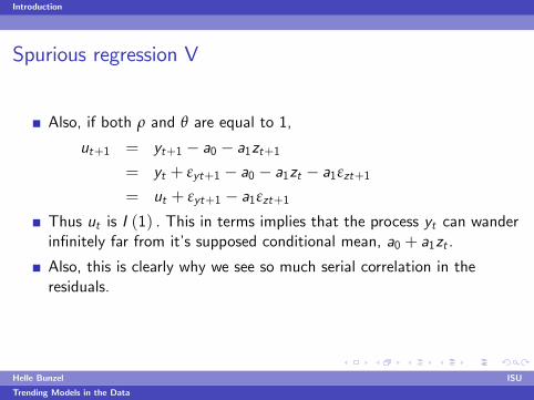
Also, if both ρ and θ are equal to 1,

ut+1 = yt+1 � a0 � a1zt+1= yt + εyt+1 � a0 � a1zt � a1εzt+1= ut + εyt+1 � a1εzt+1

Thus ut is I (1) . This in terms implies that the process yt can wanderin�nitely far from it�s supposed conditional mean, a0 + a1zt .

Also, this is clearly why we see so much serial correlation in theresiduals.

Helle Bunzel ISU

Trending Models in the Data

Introduction

Spurious regression VIFinally there is another possibility, if ρ = θ = 1 and εyt and εzt arenot independent. Then we can write:

ut+1 = ut + εyt+1 � a1εzt+1= ut�1 + εyt + εyt+1 � a1εzt � a1εzt+1

=t+1

∑i=1

εyi � a1t+1

∑i=1

εzi

If, for example, εyt and εzt are perfectly correlated and a1 = 1, thenut+1 = 0, which is certainly stationary. Thus, yt and zt are bothI (1) , but yt � zt is stationary.This is called cointegration.To sum up: We consider the regression:

yt = a0 + a1zt + ut

Helle Bunzel ISU

Trending Models in the Data

Introduction

Spurious regression VIIIf both yt and zt are stationary, so is ut and all our usual regressiontheory holds.

If yt and zt are integrated of di¤erent orders, ut is nessesarilynon-stationary, the regression is meaningless and none of our usualtheory holds.

If both yt and zt are integrated of order 1, there are two possibilities:

They are unrelated series, but you do no nessesarily reject a1 = 0 andR2 is high. In this case ut is again non-stationary.The series are cointegrated and thus ut is stationary. How to treatthese models is a whole separate topic.

Bottomline: It is VERY important to know whether your variables areintegrated or not when you apply regression analysis.

Spurious regression, visuals:

Helle Bunzel ISU

Trending Models in the Data

Introduction

Spurious regression VIII

Helle Bunzel ISU

Trending Models in the Data

Introduction

Spurious regression IX

Helle Bunzel ISU

Trending Models in the Data

Introduction

Distinguishing Di¤erent Models I

Consider the following data from four di¤erent models:

Helle Bunzel ISU

Trending Models in the Data

Introduction

Distinguishing Di¤erent Models II

It is clear that we cannot tell these apart by visual inspection.

Will the ACF tell us that we are dealing with a unit root process?Consider the simple example:

yt = yt�1 + εt ,

yt = y0 +t

∑j=1

εj

and

E (yt ) = y0

Helle Bunzel ISU

Trending Models in the Data

Introduction

Distinguishing Di¤erent Models III

The autocovariance is:

γs = E [(yt � y0) (yt�s � y0)]

= E

"t

∑j=1

εjt�s∑i=1

εi

#= (t � s) σ2

The variance is:

V (yt ) = tσ2

and therefore the ACF is

ρs =(t � s)p(t � s) t

=

r(t � s)t

Helle Bunzel ISU

Trending Models in the Data

Introduction

Distinguishing Di¤erent Models IV

Note that as s increases the ACF falls, making it hard to tell thedi¤erence between the unit root process and an AR process, evenwhen the errors are white noise.

For a trend model:

yt = α+ δt + ut

E (yt ) = α+ δt

and

V (yt ) = V (ut )

Helle Bunzel ISU

Trending Models in the Data

Introduction

Distinguishing Di¤erent Models V

So

γs = E [(yt � (α+ δt)) (yt�s � (α+ δ (t � s)))]= E (utut�s )

and

ρs =E (utut�s )V (ut )V (us )

So the ACF re�ects the ACF of the error process. Clearly recognizableif the error process is white noise...

The �rst investigation to distinguish between these two types of serieswas made using the ACF of the residuals series �tted to eitherstochastic or deterministic trends.

Helle Bunzel ISU

Trending Models in the Data

Introduction

Distinguishing Di¤erent Models VIConsider the following estimation on real GDP data:

rgdpt = 2.224+ 0.385t � 0.0002t2 + 1.85 � 10�6t3

The graph of the data and the �tted values looks like:

Helle Bunzel ISU

Trending Models in the Data

Introduction

Distinguishing Di¤erent Models VII

If we just eyeball, this seems like a very good model.

An alternative estimation is:

∆ ln (rgdpt ) = 0.005+ 0.256∆ ln (rgdpt�1) + 0.1496∆ ln (rgdpt�2)

The ACF and PACF from the residuals look like:

Helle Bunzel ISU

Trending Models in the Data

Introduction

Distinguishing Di¤erent Models VIII

Helle Bunzel ISU

Trending Models in the Data

Introduction

Distinguishing Di¤erent Models IX

Clearly there is a lot of persistence left after de-trending, even thoughthe �t looked very good, where as the estimated unit root modelseems to have residuals that behave like white noise.

This point was �rst made by Nelson and Plosser in 1982. They �ttedthirteen important macroeconomic series that had been treated astrend-stationary up until that point.

Helle Bunzel ISU

Trending Models in the Data

Introduction

Unit Root Testing in a Simple Model I

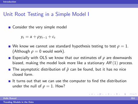
Consider the very simple model

yt = α+ ρyt�1 + εt

We know we cannot use standard hypothesis testing to test ρ = 1.(Although ρ = 0 would work).

Especially with OLS we know that our estimates of ρ are downwardsbiased, making the model look more like a stationary AR (1) process.

The asymptotic distribution of ρ can be found, but it has no niceclosed form.

It turns out that we can use the computer to �nd the distributionunder the null of ρ = 1. How?

Helle Bunzel ISU

Trending Models in the Data

Introduction

Unit Root Testing in a Simple Model IIYou generate data according to

yt = α+ yt�1 + εt

Then you estimate

yt = α+ ρyt�1 + εt

using OLS and record the value of ρ and s2, or, more importantly

t =ρ� 1q

s2 ∑ (yt�1 � y)2

You repeat this process many times and keep the results.

Helle Bunzel ISU

Trending Models in the Data

Introduction

Unit Root Testing in a Simple Model IIIDickey and Fuller found that

90% of the time t was less than 2.5895% of the time t was less than 2.8999% of the time t was less than 3.51

How do you use this information to carry out tests?

What type of mistake would we have been making if we usedstandard normal critical values?

How would you create a two-sided test?

Caution: These methods only work if a CLT actually applies!

It is also nessesary to investigate how the assumptions under whichyou generated the data a¤ects the reults. In this case:

Do the numbers depend on the exact distribution of εt ?Do the numbers depend on the value of α used to generate the data?

Helle Bunzel ISU

Trending Models in the Data

Introduction

Dickey-Fuller Tests I

A little about Dickey and Fuller and Iowa State.

Dickey and Fuller considered three di¤erent models:

∆yt = γyt�1 + εt (1)

∆yt = a0 + γyt�1 + εt (2)

∆yt = a0 + γyt�1 + a2t + εt (3)

Note that (1) is equivalent to the model we considered last section.

The hypothesis of interest now is H0 : γ = 0.

The alternative we are considering is HA : γ < 0.

Typically we ignore the possibility that yt = �yt�1 + εt , even though,stricly speaking, this is also a unit root.

Helle Bunzel ISU

Trending Models in the Data

Introduction

Dickey-Fuller Tests II

To test γ = 0, we simply calculate the standard t � statistic .Unfortunately the critical values are di¤erent for the three di¤erentmodels above.

The t-test statitistic for the three models above are ususally labelled:τ, τµ and ττ.

Dickey and Fuller also provide critical values for F � test of jointhypotheses in these three models. We will apply these in an examplelater.

Helle Bunzel ISU

Trending Models in the Data

Introduction

Augmented Dickey-Fuller Tests I

Clearly AR (1) models are not always su¢ cient to describe our data.

Consider an AR (p) process:

yt = a0 + a1yt�1 + a2yt�2 + ...+ apyt�p + εt

We can rewrite this model in the following way:

yt = a0 + a1yt�1 + ...

+ap�1yt�p+1 + apyt�p+1 � ap∆yt�p+1 + εt

= a0 + a1yt�1 + ...

+ (ap�1 + ap) yt�p+1 � ap∆yt�p+1 + εt

= a0 + a1yt�1 + ...+ ap�2yt�p+2 + (ap�1 + ap) yt�p+2� (ap�1 + ap)∆yt�p+2 � ap∆yt�p+1 + εt

Helle Bunzel ISU

Trending Models in the Data

Introduction

Augmented Dickey-Fuller Tests II

yt = a0 + a1yt�1 + ...+ (ap�2 + ap�1 + ap) yt�p+2� (ap�1 + ap)∆yt�p+2 � ap∆yt�p+1 + εt

= a0 + (a1 + ...+ ap�1 + ap) yt�1� (a2 + ...+ ap�1 + ap)∆yt�1 � ...� ap∆yt�p+1 + εt

From this expression we get:

∆yt = a0 + (a1 + ...+ ap�1 + ap � 1) yt�1� (a2 + ...+ ap�1 + ap)∆yt�1 � ...� ap∆yt�p+1 + εt

= a0 + γyt�1 +p

∑i=2

βi∆yt�i+1 + εt

Helle Bunzel ISU

Trending Models in the Data

Introduction

Augmented Dickey-Fuller Tests IIIwhere

γ =

p

∑i=1ai

!� 1 and

βi = �p

∑j=iaj

Again, we have a unit root if γ = 0.

If this model is correctly speci�ed we can use the critical values whichapplied to the simpler models.

Helle Bunzel ISU

Trending Models in the Data

Introduction

Augmented Dickey-Fuller Tests IVThis still leaves many important issues to deal with in the data:

The model may contain unknown MA components.We need to have the right number of autoregressive lags.The data might be I (2) or higher.There might be structural breaks in the data. These can confuse andmake it seem like otherwise stationary data has a unit root.We may not know whether to include the constant and trend in themodel.

Unknown MA components are reaonable simple to deal with. We canwrite an invertible ARMA process as an AR (∞) process, such that:

∆yt = a0 + γyt�1 +∞

∑i=2

βi∆yt�i+1 + εt

This we cannot estimate with �nite samples....

Helle Bunzel ISU

Trending Models in the Data

Introduction

Augmented Dickey-Fuller Tests V

Dickey and Fuller have shown that an unknown ARIMA (p, 1, q)process can be well approximated by an ARIMA (n, 1, 0) , where

n � T 13 . Clearly we can estimate an ARIMA

�T

13 , 1, 0

�with a

dataset of T observations.

Helle Bunzel ISU

Trending Models in the Data

Introduction

Augmented Dickey-Fuller Tests ILag-length Selection

An important practical issue for the implementation ofthe ADF test isthe speci�cation of the lag length p.

If p is too small then the remaining serial correlation in the errors willbias the test.If p is too large then the power of the test will su¤er. (Why?)

Monte Carlo experiments suggest it is better to err on the side ofincluding too many lags.

A standard method for lag selection is:

Set an upper bound pmax for p.Estimate the ADF test regression with p = pmax .

Helle Bunzel ISU

Trending Models in the Data

Introduction

Augmented Dickey-Fuller Tests IILag-length Selection

If the absolute value of the t � statistic for testing the signi�cance ofthe last lagged di¤erence is greater than 1.6 then set p = pmax andperform the unit root test. Otherwise, reduce the lag length by one andrepeat the process.A common rule of thumb for determining pmax , suggested by Schwert(1989), is

pmax =

"12�T100

� 14#

where [x ] denotes the integer part of x .Note that this choice is completely ad hoc!

Remember to check that the residuals look like white noise afterselecting a lag length (regardless of selection method....)

Helle Bunzel ISU

Trending Models in the Data

Introduction

Augmented Dickey-Fuller Tests IIILag-length Selection

A di¤erent way to determine lag length is to use information criteria.The standard AIC and SBC are often used.

Example of lag length selection.

200 observations were generated by:

∆yt = 0.5+ 0.5∆yt�1 + 0.2∆yt�3 + εt

Here the series does contain a unit root and the correct lag length is 3.

The data looks like:

Helle Bunzel ISU

Trending Models in the Data

Introduction

Augmented Dickey-Fuller Tests IVLag-length Selection

Helle Bunzel ISU

Trending Models in the Data

Introduction

Augmented Dickey-Fuller Tests VLag-length Selection

Seeing this data we clearly cannot tell whether or not to include atrend, so we estimate:

∆yt = a0 + a2t + γyt�1 +p

∑i=2

βi∆yt�i+1 + εt

The estimation results are:

Helle Bunzel ISU

Trending Models in the Data

Introduction

Augmented Dickey-Fuller Tests VILag-length Selection

For this model the critical value for the DF test is �3.43. (Reject ift � test < �3.43)SBC and AIC do not agree on the lag length choice.

It turns out, however, that this does not a¤ect the conclusion of theunit root test....

The φ2 statistic tests the hypothesis that a0 = a2 = γ = 0 and theφ3 statistic tests the hypothesis that a2 = γ = 0.

The critical values are 4.88 and 6.49. As a result we do reject thepresence of a trend, but not the presence of a constant.

If we had tested this model with t and F � tests, β4 = 0,β3 = β4 = 0 and so forth, we would have concluded that we shouldhave included 2 lags.

Helle Bunzel ISU

Trending Models in the Data

Introduction

Augmented Dickey-Fuller Tests VIILag-length Selection

Also note that had we used four lags, we would not have been able toreject a0 = a2 = γ = 0. This is because of the reduced power of thetest.

Finally note that he current state of the art for lag selection wasintroduced by Ng and Perron in 2001. This critereon is theMAIC (k) .

Helle Bunzel ISU

Trending Models in the Data