Trend of Saudi Arabia Students Taking Higher Education Abroad

Trend of Saudi Arabia Students Taking

Higher Education Abroad

A THESIS

SUBMITTED TO THE GRADUATE EDUCATIONAL COUNCIL

IN PARTIAL FULFILLMENT OF THE REQUIREMENTS

For the degree

MASTER OF SCIENCE

By

Majed Saeed Alghamdi

Advisor Dr. Rahmatullah Imon

Ball State University

Muncie, Indiana

May 2016

i

Trend of Saudi Arabia Students Taking Higher Education Abroad

A THESIS

SUBMITTED TO THE GRADUATE EDUCATIONAL COUNCIL

IN PARTIAL FULFILLMENT OF THE REQUIREMENTS

FOR THE DEGREE

MASTER OF SCIENCE

By

Majed Saeed Alghamdi

Committee Approval:

…………………………………………………………………………………………….

Committee Chairman Date

……………………………………………………………………………………………

Committee Member Date

…………………………………………………………………………………………….

Committee Member Date

Department Head Approval:

……………………………………………………………………………………………

Head of Department Date

Graduate office Check:

……………………………………………………………………………………………

Dean of Graduate School

Date

Ball State University

Muncie, Indiana

May, 2016

ii

ACKNOWLEDGEMENTS

I would like to express my special appreciation and thanks to my advisor Professor Dr.

Rahmatullah Imon, you have been a tremendous mentor for me, for his patience, motivation,

enthusiasm, and immense knowledge. His guidance helped me in all the time during my analysis

and writing the report. I could not have imagined having a better advisor and mentor for my thesis

other than him I would also like to thank my committee members, professor Dr. Munni Begum

and Dr. Yayuan Xiao for their encouragement, insightful comments and patience. I am thankful to

all my classmates for their kind supports. Last but not the least, I would like to thank my family:

my parents, my brothers and sisters, for supporting me throughout my life.

Majed Alghamdi

May 7, 2016

iii

ABSTRACT

In this study our prime objective was to investigate the trend of Saudi Arabia students who are

studying abroad for higher education. We find student enrolment is growing almost exponentially

over the years. The most popular programs are Engineering and Medical Science and the least

popular programs are Agriculture and Fine Arts. We also find an evidence of gender discrimination

against women among the Saudi Arabia students studying abroad. In quest of which factors

influence the number of students studying abroad we consider regression analysis and find that

budget in higher education and oil price are the most important variables to explain students’

enrolment. Both regression and cross validation study reveal that the robust reweighted least

squares (RLS) fit the data better than other models and yield better forecasts.

iv

Table of Contents

CHAPTER 1 .................................................................................................................................. 1

INTRODUCTION ..................................................................................................................... 1

1.1 Objective of the Study ....................................................................................................... 3

1.2 Sources of Data .................................................................................................................. 3

1.3 Methodology ...................................................................................................................... 4

CHAPTER 2 .................................................................................................................................. 5

Trend of Saudi Arabia Students Studying abroad ................................................................. 5

2.1 Trend Analysis ................................................................................................................... 5

2.2 Trend Analysis of Nine Major Programs ........................................................................ 10

2.3 Trend Analysis of Some Other Relevant Variables ......................................................... 28

2.4 Summary Results of Trend Analysis ............................................................................... 34

CHAPTER 3 ................................................................................................................................ 35

Comparison between Genders and Different Programs ..................................................... 35

3.1 Comparison between Genders ......................................................................................... 35

3.2 Tests for the Equality of Means between Male and Female Students ............................. 41

3.3 Comparison of the Individual Treatment Means ............................................................. 46

3.4 Result Summary .............................................................................................................. 48

v

CHAPTER 4 ................................................................................................................................ 50

Modeling and Fitting of Data Using Regression Diagnostics and Robust Regression ...... 50

4.1 Classical Regression Analysis ......................................................................................... 50

4.2 Regression Diagnostics .................................................................................................... 54

4.3 Robust Regression ........................................................................................................... 62

4.4 Regression Results ........................................................................................................... 65

4.5 Results Comparisons ....................................................................................................... 75

CHAPTER 5 ................................................................................................................................ 76

Cross Validation of Forecasts................................................................................................. 76

5.1 Evaluation of Forecasts by Cross Validation .................................................................. 76

5.2 Cross Validation Results ................................................................................................. 78

CHAPTER 6 ................................................................................................................................ 80

Conclusions and Areas of Further Research ........................................................................ 80

6.1 Conclusions ..................................................................................................................... 80

6.2 Areas of Further Research ............................................................................................... 81

References .................................................................................................................................... 82

APPENDIX A .............................................................................................................................. 84

APPENDIX B .............................................................................................................................. 88

vi

List of Tables

Chapter 2

Table 2.1: Trend Summary of the Total Number of Students ...................................................... 12

Table 2.2: Trend Summary of the Total Number of Social Science Students .............................. 15

Table 2.3: Trend Summary of the Total Number of Natural Science Students ............................ 17

Table 2.4: Trend Summary of the Total Number of Medical Science Students ........................... 18

Table 2.5: Trend Summary of the Total Number of Law Students .............................................. 20

Table 2.6: Trend Summary of the Total Number of Humanities Students ................................... 21

Table 2.7: Trend Summary of the Total Number of Fine Arts ..................................................... 23

Table 2.8: Trend Summary of the Total Number of Engineering Students .................................. 24

Table 2.9: Trend Summary of the Total Number of Education Students ..................................... 26

Table 2.10 Trend Summary of the Total Number of Agriculture Students .................................. 27

Table 2.11: Trend Summary of Oil Revenue ................................................................................ 30

Table 2.12: Trend Summary of Budget in Higher Education ....................................................... 32

Table 2.13: Trend Summary of Oil Price ...................................................................................... 33

Table 2.14: Trend Summary ......................................................................................................... 34

Chapter 3

Table 3.1: Summary Test Results for the Equality of Means between Male and Female Students

....................................................................................................................................................... 42

Table 3.2: Average Number of Students in Different Programs .................................................. 43

Table 3.3 ANOVA Table for the Equality of Mean Test of Nine Programs ................................ 48

vii

Chapter 4

Table 4.1: Regression Results Summary ...................................................................................... 75

Chapter 5

Table 5.1: Original and Forecasted Values for 2011-2014 ........................................................... 78

Table 5.2: Cross Validation Result Summary ............................................................................... 79

viii

List of Figures

Chapter 2

Figure 2.1: Time Series Plot of the Total Number of Students .................................................... 10

Figure 2.2: Trend Analysis of the Total Number of Students....................................................... 11

Figure 2.3: Time Series Plot of Total Number of Students in Different Programs ...................... 12

Figure 2.4: Time Series Plot of Total Number of Students (in ln) in Different Programs ........... 13

Figure 2.5: Trend Analysis Plot of the Total Number of Social Science Students ....................... 15

Figure 2.6: Trend Analysis Plot of the Total Number of Students for Natural Science ............... 16

Figure 2.7: Trend Analysis Plot of the Total Number of Students for Medical Science .............. 18

Figure 2.8: Trend Analysis Plot of the Total Number of Students for Law ................................. 19

Figure 2.9: Trend Analysis Plot of the Total Number of Students for Humanities ...................... 21

Figure 2.10: Trend Analysis Plot of the Total Number of Students for Fine Arts ....................... 22

Figure 2.11: Trend Analysis Plot of the Total Number of Students for Engineering ................... 24

Figure 2.12: Trend Analysis Plot of the Total Number of Students for Education ...................... 25

Figure 2.13: Trend Analysis Plot of the Total Number of Students for Agriculture .................... 27

Figure 2.14: Time Series Plot of the Budget in Higher Education ............................................... 28

Figure 2.15: Time Series Plot of Oil Price .................................................................................... 28

Figure 2.16: Time Series Plot of Oil Revenue .............................................................................. 29

Figure 2.17: Trend Analysis of Oil Revenue ................................................................................ 30

Figure 2.18: Trend Analysis of Budget in Higher Education ....................................................... 31

Figure 2.19: Trend Analysis of Oil Price ...................................................................................... 33

ix

Chapter 3

Figure 3.1: Time Series Plot of Male and Female Students in Social Science ............................. 35

Figure 3.2: Time Series Plot of Male and Female Students in Natural Science ........................... 36

Figure 3.3: Time Series Plot of Male and Female Students in Medical Science .......................... 37

Figure 3.4: Time Series Plot of Male and Female Students in Law ............................................. 37

Figure 3.5: Time Series Plot of Male and Female Students in Humanities .................................. 38

Figure 3.6: Time Series Plot of Male and Female Students in Engineering ................................. 39

Figure 3.7: Time Series Plot of Male and Female Students in Education .................................... 39

Figure 3.8: Time Series Plot of Male and Female Students in Fine Arts ..................................... 40

Figure 3.9: Time Series Plot of Male and Female Students in Agriculture .................................. 40

Figure 3.10: Box Plot of Number of Students in Different Programs .......................................... 43

Chapter 4

Figure 4.1: Scatter Plot of the Total Number of Students vs Budget in Higher Education .......... 66

Figure 4.2: Scatter Plot of the Total Number of Students vs Oil Price ......................................... 67

Figure 4.3: RLS and OLS Fit of the Total Number of Students vs Oil Price ............................... 67

Figure 4.4: Scatter Plot of the Total Number of Students vs Oil Revenue ................................... 68

Figure 4.5: Normal Probability Plot of the Residuals for Model A .............................................. 72

Figure 4.6: Normal Probability Plot of the Residuals for Model B .............................................. 73

Figure 4.7: Normal Probability Plot of the Residuals for Model C .............................................. 74

Chapter 5

Figure 5.1: Scatterplot of RLS, OLS, Exponential Forecasts vs Original Values ........................ 78

1

CHAPTER 1

INTRODUCTION

As early as the reign of King Abdulaziz, The founding king of Saudi Arabia, students were being

sponsored to study abroad. Early programs were limited to Arab countries such as Egypt and

Lebanon to study Arabic and Islamic studies. The number of Saudi Arabian students studying

abroad has increased dramatically during the past decade. This explosive growth can be

attributed to an educational agreement brokered between former U.S. president George Bush and

Saudi King Abdullah bin Abdulaziz Al Saud in 2005. The agreement opened the doors for Saudi

students to pursue their higher educational degrees in the U.S. with their government paying all

of their educational expenses. As a result over 100,000 Saudi students were enrolled in American

colleges and universities in 2013-14, making Saudi Arabia the fourth largest sponsor of

international students to the U.S.

Saudi enrollments overseas have been growing exponentially since the 2005 introduction of

the King Abdullah bin Abdulaziz Scholarship Program (KASP). In 2012, the KASP was extended

with the aim of helping a further 50,000 Saudis graduate from the world’s top 500 universities by

2020. According to data from the Institute for International Education, in the 2012/13 academic

year there were a total of 44,586 tertiary-level Saudi students in the United States, an almost 100

percent increase from 2010/11 and a 12-fold increase from 2005.

The most recent data from the Student and Exchange Visitor Program’s SEVIS database show that

there were a total of 70,366 active nonimmigrant Saudi students (including dependents) in the

http://www.mohe.gov.sa/en/studyaboard/King-Abdulla-hstages/Pages/default.aspx

2

United States in July 2014 on F, J or M visas. This compares to 61,944 at the same time in

2013. Saudi government data pegs the 2013/14 number of Saudi students and dependents in the

United States at a significantly larger 106,858. Of those 89,423 were reported to be on government

scholarships. The same data show that there were 20,252 students in the United Kingdom, 18,926

in Canada, and 13,002 in Australia, with just under 200,000 total Saudi students at institutions

abroad (75% male) across the world.

By level of study, 120,000 students are at the undergraduate level, 47,500 at the master’s level and

10,400 at the doctoral level. The KASP will continue to prioritize fields designated as important

to progressing the Saudi “knowledge economy,” such as medicine, engineering and science.

Approximately 70 percent of scholarship students currently study in subjects related to Business

Administration, Engineering, Information Technology and Medicine. The top fields of study for

Saudi students in the United States last year were: Intensive English (27.2%), Engineering

(21.1%), Business/Management (17.1%), Math and Computer Science (7.4%), and Health

Professions (5.6%).

The Saudi government is projected to invest over 10% of its annual budget to higher education for

the foreseeable future. Currently it invests nearly $2.4 billion in the KASP initiative annually,

which includes academic funding as well as living expenses for over 100,000 students enrolled in

graduate and undergraduate programs in the U.S. If the Saudi government continues to support

KASP at the current level, it will soon surpass South Korea in terms of sending more students

abroad to study

3

1.1 Objective of the Study


studying abroad for higher education. We would like to investigate both the overall trend and also

trends of individual programs. We would like to see whether there is any special preference for

any particular program. Another point of our interest is to investigate whether there is any gender

discrimination among the students? We would also like to find out the most important factors that

influence the number of students studying abroad most. We would employ regression analysis for

this and for the validity of the model we would employ recent diagnostics. If the conventionally

used least squares method fails we would either use robust regression or choose some other models.

To confirm which method does fit the data best we would apply cross validation.

1.2 Sources of Data

The most important data I need for my study is the number of Saudi Arabia students studying

abroad for higher education. This data set is taken from the official website The Ministry of Higher

Education of Saudi Arabia as given below.

https://www.mohe.gov.sa/ar/Ministry/Deputy-Ministry-for-Planning-and-Information-

affairs/HESC/Ehsaat/Pages/default.aspx

We have data for both male and female students in nine programs from 1981-2014. The nine

programs are Social Science, Natural Science, Medical Science, Law, Humanities, Fine Arts,

Engineering, Education, and Agriculture.

We believe that Budget in Higher Education is a key factor to understand the number of Saudi

Arabia students studying abroad. The Budget in Higher Education data set from 1981 to 2014 is

https://www.mohe.gov.sa/ar/Ministry/Deputy-Ministry-for-Planning-and-Information-affairs/HESC/Ehsaat/Pages/default.aspx


4

taken from the official website of the Ministry of Finance of Saudi Arabia. Here is the link of the

data:

https://www.mof.gov.sa/english/DownloadsCenter/Pages/Budget.aspx

We know Saudi Arabia heavily relies on Oil. We feel Oil Revenue and Oil Price could be very

important variables for our study. We collect these data from 1981-3014 from the official website

of Saudi Arabian Moneytary Agency (SAMA). Here is the link of the data:

http://www.sama.gov.sa/en-US/EconomicReports/Pages/YearlyStatistics.aspx

All these data are presented in Appendix A of my thesis.

1.3 Methodology

In this study we have employed a number of modern and sophisticate statistical techniques. We

have used linear, quadratic and exponential trend models to investigate both the overall trend and

also trends of individual programs. We have used experimental design technique to see whether

there is any special preference for any particular program and to investigate whether there is any

gender discrimination among the students. We would also like to find out the most important

factors that influence the number of students studying abroad most. We employ Fisher’s LSD and

Tukey’s test in this regard. We employ recent diagnostics like Jarque-Bera and Rescaled Moments

for normality and the robust reweighted least squares (RLS) technique for regression analysis.

Finally we employ a cross validation study based on the mean squared percentage error (MSPE)

to confirm which method does fit the data best.



5

CHAPTER 2

Trend of Saudi Arabia Students Studying abroad

In this chapter we introduce different time series models that we are going to use in our study with

their estimation procedures and properties. An excellent review of different aspects of time series

models are available in Pyndick and Rubenfield (1998), Bowerman et al. (2005), Montgomery et

al. (2008) and estimation. A time series is a chronological sequence of observations on a particular

variable. A time series model accounts for patterns of the past movement of a variable and uses

that information to predict its future movements, i.e., it is a sophisticated method of extrapolating

data. There are two different approaches of modeling a time series data: deterministic and

stochastic.

2.1 Trend Analysis

We begin with simple models that can be used to forecast a time series on the basis of its past

behavior. Most of the series we encounter are not continuous in time, instead, they consist of

discrete observations made at regular intervals of time. We denote the values of a time series by {

ty }, t = 1, 2, …, T. Our objective is to model the series ty and use that model to forecast ty beyond

the last observation Ty . We denote the forecast l periods ahead by lTy ˆ .

We sometimes can describe a time series ty by using a trend model defined as

ttty TR (2.1)

where tTR is the trend in time period t.

6

2.1.1 Linear Trend Model:

tt 10TR (2.2)

We can predict ty by

tyt 10

ˆˆˆ (2.3)

Then the forecast l period ahead is given by

lTy lT 10ˆˆˆ

(2.4)

For this particular model the distance value is DV =

T

t

tt

tlT

T

1

2

21

. Hence the 100(1– )%

prediction interval for an individual value of the dependent variable DV1ˆ2/,2 sty TlT .

2.1.2 Polynomial Trend Model of Order p

p

pt ttt ...TR 2

210 (2.5)

If the number of observation is not too large, we can predict ty by

p

pt ttt ˆ...ˆˆˆy 2

210 (2.6)


p

plT lTlTlT ˆ...ˆˆˆy2

210 (2.7)

The 100(1– )% prediction interval for an individual value of the dependent variable

DV1ˆ2/,1 sty pTlT (2.8)

7

Quadratic Trend Model:

It is a special case of polynomial trend model when order p = 2. Hence from the above results we

have

2

210TR ttt (2.9)

If the number of observation is not too large, we can predict ty by

2

210ˆˆˆy ttt

(2.10)


2

210ˆˆˆy lTlTlT

(2.11)

The 100(1– )% prediction interval for an individual value of the dependent variable

DV1ˆ2/,3 sty TlT (2.12)

2.1.3 Comparisons of Different Methods

Minitab computes three measures of accuracy of the fitted model: MAPE, MAD, and MSD for

each of the simple forecasting and smoothing methods. For all three measures, the smaller the

value, the better the fit of the model. Use these statistics to compare the fits of the different

methods.

MAPE, or Mean Absolute Percentage Error, measures the accuracy of fitted time series values. It

expresses accuracy as a percentage.

MAPE =

100|/ˆ|

T

yyy ttt

(2.13)

8

where ty equals the actual value, ty equals the fitted value, and T equals the number of

observations.

MAD (Mean), which stands for Mean Absolute Deviation, measures the accuracy of fitted time

series values. It expresses accuracy in the same units as the data, which helps conceptualize the

amount of error.

MAD (Mean) = T

yy tt |ˆ|

(2.14)


observations.

MSD stands for Mean Squared Deviation. MSD is always computed using the same denominator,

T, regardless of the model, so you can compare MSD values across models. MSD is a more

sensitive measure of an unusually large forecast error than MAD.

MSD =

T

yy tt 2

ˆ

(2.15)


observations.

2.1.4 Exponential smoothing

Exponential smoothing provides a forecasting method that is most effective when the components

of the time series may be changing over time. It is often more reasonable to have more recent

values of ty play a greater role than do earlier values. In such a case recent values should be

weighted more heavily in the moving average.

9

Suppose that the time series ty has a level (or mean) that may slowly change over time but has no

trend or seasonal pattern. This series can be described as

tty 0 (2.16)

Then the estimate T for the level of the series in time period T is given by the smoothing equation

11 TTT y (2.17)

where is a smoothing constant between 0 and 1, and 1T is the estimate of the level in the time

period T – 1.

A point forecast for one period ahead us given by

TTy 1ˆ

(2.18)

which implies

1ˆ

Ty = ...11 2

2

1 TTT yyy =

0

1

Ty

(2.19)

It is easy to show that the l period forecast lTy ˆ can be given by

lTy ˆ =

0

1

Ty

(2.20)

There are several methods to choose the appropriate value of . The most popular method is to

choose which minimizes the mean sum of (squared) distances (MSD) of the actual and

forecasted values. Other measures of accuracy are the mean absolute percentage error (MAPE)

and the mean absolute deviation (MAD).

10

2.2 Trend Analysis of Nine Major Programs

In this section we would like to investigate trend of total number of students studying abroad in

nine major programs. For each program we consider three different trend models: linear, quadratic,

and exponential. We also compute MAPE, MAD and MSD to evaluate which method better fits

the data.

2.2.1 All Programs

At first we consider the total number of students studying abroad in all programs. Figure 2.1 gives

the time series plot of the total number of students from 1980 to 2014. From this figure it is clear

that the number of students studying abroad has an increasing trend. It seems to us that this increase

is not linear, it is exponential.

2010200520001995199019851980

100000

80000

60000

40000

20000

0

Year

Tota

l

Time Series Plot of Total No. of Students

Figure 2.1: Time Series Plot of the Total Number of Students

Now we would like to fit this data by three trend models: linear, quadratic and exponential and

the graphs are presented in Figure 2.2.

11

3330272421181512963

100000

75000

50000

25000

0

Index

Tota

l

MAPE 208

MAD 17431

MSD 439097288

Accuracy Measures

Actual

Fits

Variable

Trend Analysis Plot for TotalLinear Trend Model

Yt = -17044 + 2139*t

3330272421181512963

100000

80000

60000

40000

20000

0

Index

Tota

l

MAPE 119

MAD 8259

MSD 110484665

Accuracy Measures

Actual

Fits

Variable

Trend Analysis Plot for TotalQuadratic Trend Model

Yt = 27234 - 5241*t + 210.8*t**2

3330272421181512963

100000

80000

60000

40000

20000

0

Index

Tota

l

MAPE 77

MAD 12364

MSD 505301336

Accuracy Measures

Actual

Fits

Variable

Trend Analysis Plot for TotalGrowth Curve Model

Yt = 2054.90 * (1.0895**t)

Figure 2.2: Trend Analysis of the Total Number of Students

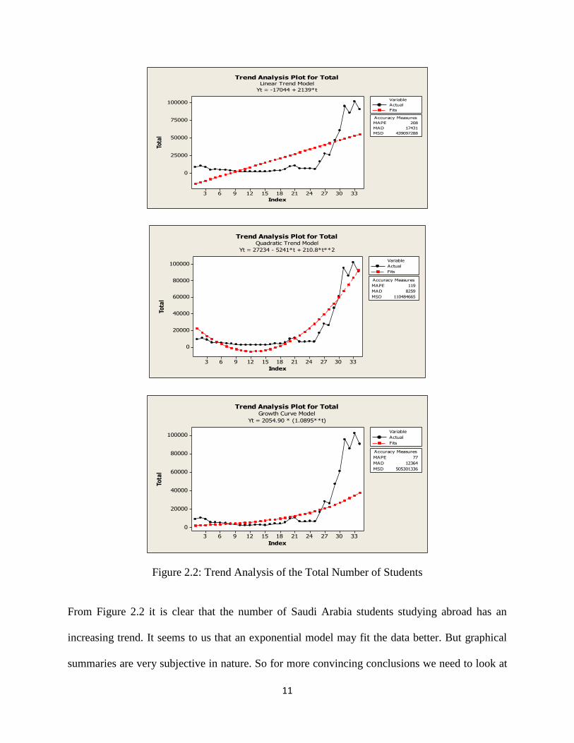
From Figure 2.2 it is clear that the number of Saudi Arabia students studying abroad has an

increasing trend. It seems to us that an exponential model may fit the data better. But graphical

summaries are very subjective in nature. So for more convincing conclusions we need to look at

12

numerical quantities. The following table gives a summary result to compare three different trend

models.

Table 2.1: Trend Summary of the Total Number of Students

Model MAPE MAD MSD

Linear 208 17431 439097288

Quadratic 119 8259 110484665

Exponential 77 12364 505301336

Results presented in Table 2.1 clearly show that both the quadratic trend model and the exponential

trend model fit the data better than the linear model but in terms of MAPE the exponential trend

model is better than the other two models.

Now we will investigate trend models for nine separate programs.

2010200520001995199019851980

35000

30000

25000

20000

15000

10000

5000

0

Year

Da

ta

Agriculture

Education

Engineering

Fine Arts

Humanities

Law

Medical Science

Natural Science

Social Science

Variable

Time Series Plot of Students in Different Programs

Figure 2.3: Time Series Plot of Total Number of Students in Different Programs

13

Figure 2.3 shows that the number of Saudi Arabia students studying abroad in each different

programs has an overall increasing trend. But there are huge differences in the number of students

so when they are plotted together some programs are not distinguishable at all. As a remedy to this

problem we plot the same graph in natural log scale and the graph is presented in Figure 2.4.

2010200520001995199019851980

11

10

9

8

7

6

5

4

3

Year

Da

ta

Agriculture

Education

Engineering

Fine Arts

Humanities

Law

Medical Science

Natural Science

Social Science

Variable

Time Series Plot of Students in Different Programs (in ln)

Figure 2.4: Time Series Plot of Total Number of Students (in ln) in Different Programs

Figure 2.3 shows that the number of Saudi Arabia students studying abroad in each different

programs has an overall increasing trend. But there are huge differences in the number of students

so when they are plotted together some programs are not distinguishable at all. As a remedy to this

problem we plot the same graph in natural log scale and the graph is presented in Figure 2.4. It is

clear from this figure that the number of students differs significantly from one program to another.

The highest enrolled programs are Engineering, Natural Science, Medical Science and Social

Science. But the number of students in Social Science dropped in the last few years. The programs

which have relatively less number of students are Agriculture and Fine Arts.

14

3330272421181512963

35000

30000

25000

20000

15000

10000

5000

0

Index

Tota

l

MAPE 112

MAD 2595

MSD 30241525

Accuracy Measures

Actual

Fits

Variable

Trend Analysis Plot for The Total of Social SceiencesQuadratic Trend Model

Yt = 3155 - 503*t + 22.6*t**2

3330272421181512963

35000

30000

25000

20000

15000

10000

5000

0

Index

Tota

l

MAPE 234

MAD 3537

MSD 34029670

Accuracy Measures

Actual

Fits

Variable

Trend Analysis Plot for The Total of Social SceiencesLinear Trend Model

Yt = -1599 + 289*t

Now we will investigate trend models for nine separate programs.

2.2.2 Social Sciences

Among the nine programs at first we consider the total number of students studying abroad in

Social Science program. Figure 2.5 gives linear, quadratic and exponential trend fits for the Social

Science program.

From the figure it is clear that the number of students studying abroad in Social Science program

shows an increasing trend. It seems to us that an exponential model may fit the data. The following

table gives a summary result to compare three different trend models.

15

3330272421181512963

35000

30000

25000

20000

15000

10000

5000

0

Index

Tota

l

MAPE 93

MAD 2552

MSD 39771799

Accuracy Measures

Actual

Fits

Variable

Trend Analysis Plot for The Total of Social SceiencesGrowth Curve Model

Yt = 658.094 * (1.0530**t)

Figure 2.5: Trend Analysis Plot of the Total Number of Social Science Students

Table 2.2: Trend Summary of the Total Number of Social Science Students

Model MAPE MAD MSD

Linear 234 3537 34029670

Quadratic 112 2595 30241525

Exponential 93 2552 39771799

Results presented in Table 2.2 clearly show that the exponential trend model fits the data better

than the other two models.

2.2.3 Natural Sciences

Our next example is the total number of students studying abroad in Natural Science program.

Figure 2.6 gives linear, quadratic and exponential trend fits for the Natural Science program. From

the figure it is clear that the number of students studying abroad in Natural Science program has

an increasing trend and an exponential model may better fit the data.

16

3330272421181512963

30000

25000

20000

15000

10000

5000

0

-5000

Index

Tota

l

MAPE 278

MAD 4086

MSD 27110563

Accuracy Measures

Actual

Fits

Variable

Trend Analysis Plot for the Total of Natural SciencesLinear Trend Model

Yt = -4613 + 508*t

3330272421181512963

30000

25000

20000

15000

10000

5000

0

Index

Tota

l

MAPE 193

MAD 2392

MSD 8401020

Accuracy Measures

Actual

Fits

Variable

Trend Analysis Plot for the Total of Natural SciencesQuadratic Trend Model

Yt = 5952 - 1252*t + 50.31*t**2

3330272421181512963

30000

25000

20000

15000

10000

5000

0

Index

Tota

l

MAPE 72

MAD 2666

MSD 30860217

Accuracy Measures

Actual

Fits

Variable

Trend Analysis Plot for the Total of Natural SciencesGrowth Curve Model

Yt = 279.595 * (1.1053**t)

Figure 2.6: Trend Analysis Plot of the Total Number of Students for Natural Science

17

3330272421181512963

30000

25000

20000

15000

10000

5000

0

-5000

Index

Tota

l

MAPE 249

MAD 4015

MSD 25461692

Accuracy Measures

Actual

Fits

Variable

Trend Analysis Plot for the Total of Medical ScienceLinear Trend Model

Yt = -4742 + 528*t

3330272421181512963

30000

25000

20000

15000

10000

5000

0

Index

Tota

l

MAPE 165

MAD 2250

MSD 7351186

Accuracy Measures

Actual

Fits

Variable

Trend Analysis Plot for the Total of Medical ScienceQuadratic Trend Model

Yt = 5652 - 1205*t + 49.50*t**2

Table 2.3: Trend Summary of the Total Number of Natural Science Students

Model MAPE MAD MSD

Linear 278 4086 27110563

Quadratic 193 2392 8401020

Exponential 72 2666 30860217



2.2.4 Medical Science

Our next example is the total number of students studying abroad in Medical Science program.

Figure 2.7 gives linear, quadratic and exponential trend fits of this data. From the figure it is clear

that the number of students studying abroad in natural science program has an increasing trend and

an exponential model may better fit the data.

18

3330272421181512963

30000

25000

20000

15000

10000

5000

0

Index

Tota

l

MAPE 61

MAD 2408

MSD 25015184

Accuracy Measures

Actual

Fits

Variable

Trend Analysis Plot for the Total of Medical ScienceGrowth Curve Model

Yt = 259.904 * (1.1148**t)

Figure 2.7: Trend Analysis Plot of the Total Number of Students for Medical Science

Table 2.4: Trend Summary of the Total Number of Medical Science Students

Model MAPE MAD MSD

Linear 249 4015 25461692

Quadratic 165 2250 7351186

Exponential 61 2408 25015184



2.2.5 Law

Here we consider the total number of students studying abroad in law program. Figure 2.8 gives

linear, quadratic and exponential trend fits of this data. From the figure it is clear that the number

of students studying abroad in Law program has an increasing trend and an exponential model may

better fit the data.

19

Figure 2.8: Trend Analysis Plot of the Total Number of Students for Law

20

Table 2.5: Trend Summary of the Total Number of Law Students

Model MAPE MAD MSD

Linear 563 657 644213

Quadratic 357 338 174624

Exponential 96 419 755189



2.2.6 Humanities

Now we consider the total number of students studying abroad in Humanities program. Figure 2.9

gives linear, quadratic and exponential trend fits of this data. From the figure it is clear that the

number of students studying abroad in Humanities program has an increasing trend. We also

observe from this plot that both quadratic and exponential models adequately fit the data.

21

Figure 2.9: Trend Analysis Plot of the Total Number of Students for Humanities

Table 2.6: Trend Summary of the Total Number of Humanities Students

Model MAPE MAD MSD

Linear 167 1179 2573862

Quadratic 58 752 1348197


Results presented in Table 2.6 clearly show that the quadratic trend model fits the data better than

the other two models.

22

2.2.7 Fine Arts

Now we consider the total number of students studying abroad in Fine Arts program. Figure 2.10


number of students studying abroad in Fine Arts program has an increasing trend and an

exponential model may better fit the data

Figure 2.10: Trend Analysis Plot of the Total Number of Students for Fine Arts

23

Table 2.7: Trend Summary of the Total Number of Fine Arts

Model MAPE MAD MSD

Linear 224.2 194.6 71151.6

Quadratic 180.2 132.1 29439.3

Exponential 69.5 126.9 84233.2



.

2.2.8 Engineering

Now we consider the total number of students studying abroad in Engineering program. Figure

2.11 gives linear, quadratic and exponential trend fits of this data. From the figure it is clear that

the number of students studying abroad in Engineering program has an increasing trend. We also

observe from this plot that an exponential model may better fit the data.

.

24

Figure 2.11: Trend Analysis Plot of the Total Number of Students for Engineering

Table 2.8: Trend Summary of the Total Number of Engineering Students

Model MAPE MAD MSD

Linear 397 4738 36869030

Quadratic 258 2724 11068847

Exponential 119 3466 50802116



25

2.2.9 Education

Now we consider the total number of students studying abroad in Education program. Figure 2.12


number of students studying abroad in Education program has an increasing trend. We also observe

from this plot that both quadratic and exponential models adequately fit the data.

Figure 2.12: Trend Analysis Plot of the Total Number of Students for Education

26

Table 2.9: Trend Summary of the Total Number of Education Students

Model MAPE MAD MSD

Linear 134 577 464455

Quadratic 48 301 214264




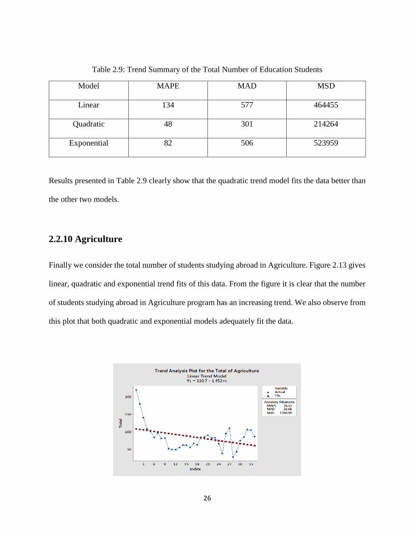
2.2.10 Agriculture

Finally we consider the total number of students studying abroad in Agriculture. Figure 2.13 gives

linear, quadratic and exponential trend fits of this data. From the figure it is clear that the number

of students studying abroad in Agriculture program has an increasing trend. We also observe from

this plot that both quadratic and exponential models adequately fit the data.

27

Figure 2.13: Trend Analysis Plot of the Total Number of Students for Agriculture

Table 2.10 Trend Summary of the Total Number of Agriculture Students

Model MAPE MAD MSD

Linear 36.53 26.68 1190.99

Quadratic 28.773 20.265 610.926

Exponential 33.25 25.90 1214.57



28

2.3 Trend Analysis of Some Other Relevant Variables

Here we consider some other variables which we believe may have a significant impact on the

number of students studying abroad. These variables are budget in higher education, oil price and

oil revenue. Oil is the key factor of Saudi Arabia economy, so oil price and oil revenue should

affect almost all major policies of the government.

At first we would like to see the trend of these variables. Time series plots of these three variables

are presented in Figures 2.14 to 2.16.

2011200620011996199119861981

2.0000E+11

1.5000E+11

1.0000E+11

5.0000E+10

0

Year

Budg

ei in

HE

Time Series Plot of Budgei in HE

Figure 2.14: Time Series Plot of the Budget in Higher Education

We observe from this figure that the budget in higher education has a steady progress over the

years and it clearly shows an increasing trend. Oil price dropped once but gained later and thus

shows an upward trend overall. Oil revenue also shows an increasing pattern.

2011200620011996199119861981

100

90

80

70

60

50

40

30

20

10

Year

Oil P

rice

Time Series Plot of Oil Price

Figure 2.15: Time Series Plot of Oil Price

29

2011200620011996199119861981

1200000

1000000

800000

600000

400000

200000

0

Year

Oil R

even

ue

Time Series Plot of Oil Revenue

Figure 2.16: Time Series Plot of Oil Revenue

Now we fit these three variables by three different trend models.

2.3.1 Oil Revenue

At first we consider oil revenue over the years. Figure 2.17 gives linear, quadratic and exponential

trend fits of this data. From the figure it is clear that oil revenue has an increasing trend. We also

observe from this plot that both quadratic and exponential models adequately fit the data.

3330272421181512963

1200000

1000000

800000

600000

400000

200000

0

Index

Oil

Rev

enue

MAPE 8.35439E+01

MAD 1.64688E+05

MSD 4.23297E+10

Accuracy Measures

Actual

Fits

Variable

Trend Analysis Plot for Oil RevenueLinear Trend Model

Yt = -127953 + 26267*t

3330272421181512963

1200000

1000000

800000

600000

400000

200000

0

Index

Oil R

even

ue

MAPE 3.55741E+01

MAD 7.94309E+04

MSD 1.23704E+10

Accuracy Measures

Actual

Fits

Variable

Trend Analysis Plot for Oil RevenueQuadratic Trend Model

Yt = 294817 - 44194*t + 2013*t**2

30

3330272421181512963

1200000

1000000

800000

600000

400000

200000

0

Index

Oil

Rev

enue

MAPE 4.79737E+01

MAD 1.26068E+05

MSD 3.40103E+10

Accuracy Measures

Actual

Fits

Variable

Trend Analysis Plot for Oil RevenueGrowth Curve Model

Yt = 55445.0 * (1.0792**t)

Figure 2.17: Trend Analysis of Oil Revenue

Table 2.11: Trend Summary of Oil Revenue

Model MAPE MAD MSD

Linear 8.35439E+01 1.64688E+05 4.23297E+10

Quadratic 3.55741E+01 7.94309E+04

1.23704E+10

Exponential 4.79737E+01 1.26068E+05 3.40103E+10



2.3.2 Budget in Higher Education

Next we consider the budget in higher education. Figure 2.18 gives linear, quadratic and

exponential trend fits of this data. From the figure it is clear that the budget in higher education

shows an increasing trend. We also observe from this plot that both quadratic and exponential

models adequately fit the data.

31

3330272421181512963

2.0000E+11

1.5000E+11

1.0000E+11

5.0000E+10

0

Index

Bu

dg

ei i

n H

E

MAPE 5.86496E+04

MAD 1.89828E+10

MSD 5.58537E+20

Accuracy Measures

Actual

Fits

Variable

Trend Analysis Plot for Budgei in HELinear Trend Model

Yt = -38718871627 + 5497524487*t

3330272421181512963

2.0000E+11

1.5000E+11

1.0000E+11

5.0000E+10

0

Index

Bu

dg

ei i

n H

E

MAPE 1.64690E+04

MAD 8.29748E+09

MSD 1.18811E+20

Accuracy Measures

Actual

Fits

Variable

Trend Analysis Plot for Budgei in HEQuadratic Trend Model

Yt = 12499933066 - 3038942962*t + 243899070*t**2

3330272421181512963

1.0000E+12

8.0000E+11

6.0000E+11

4.0000E+11

2.0000E+11

0

Index

Bu

dg

ei i

n H

E

MAPE 5.35190E+02

MAD 8.71668E+10

MSD 3.87341E+22

Accuracy Measures

Actual

Fits

Variable

Trend Analysis Plot for Budgei in HEGrowth Curve Model

Yt = 102994932 * (1.3105**t)

Figure 2.18: Trend Analysis of Budget in Higher Education

32

Table 2.12: Trend Summary of Budget in Higher Education

Model MAPE MAD MSD

Linear 5.86496E+04 1.89828E+10 5.58537E+20

Quadratic 1.64690E+04 8.29748E+09 1.18811E+20

Exponential 5.35190E+02 8.71668E+10 3.87341E+22



2.3.3 Oil Price

Next we consider oil price. Figure 2.19 gives linear, quadratic and exponential trend fits of this

data. From the figure it is clear that oil price shows an increasing trend. We also observe from this

plot that both quadratic and exponential models adequately fit the data.

3330272421181512963

100

90

80

70

60

50

40

30

20

10

Index

Oil P

rice

MAPE 59.160

MAD 20.980

MSD 554.086

Accuracy Measures

Actual

Fits

Variable

Trend Analysis Plot for Oil PriceLinear Trend Model

Yt = 30.67 + 0.877*t

33

3330272421181512963

100

90

80

70

60

50

40

30

20

10

Index

Oil P

rice

MAPE 18.8959

MAD 7.6090

MSD 95.7177

Accuracy Measures

Actual

Fits

Variable

Trend Analysis Plot for Oil PriceQuadratic Trend Model

Yt = 82.96 - 7.838*t + 0.2490*t**2

3330272421181512963

100

90

80

70

60

50

40

30

20

10

Index

Oil

Pric

e

MAPE 48.344

MAD 19.889

MSD 565.457

Accuracy Measures

Actual

Fits

Variable

Trend Analysis Plot for Oil PriceGrowth Curve Model

Yt = 28.291 * (1.01911**t)

Figure 2.19: Trend Analysis of Oil Price

Table 2.13: Trend Summary of Oil Price

Model MAPE MAD MSD

Linear 59.160 20.980 554.086

Quadratic 18.8959 7.6090 95.7177

Exponential 48.344 19.889 565.457



34

2.4 Summary Results of Trend Analysis

In this section we summarize the above trend results. Altogether we have considered 13 variables.

Table 2.14 gives a quick view regarding which model is appropriate for which variable.

Table 2.14: Trend Summary

Variable Model Direction

Total Number of Students Exponential Increasing

Students in Social Science Exponential Increasing

Students in Natural Science Exponential Increasing

Students in Medical Science Exponential Increasing

Students in Law Exponential Increasing

Students in Humanities Quadratic Increasing

Students in Fine Arts Exponential Increasing

Students in Engineering Quadratic Increasing

Students in Education Exponential Increasing

Students in Agriculture Quadratic Increasing

Oil Revenue Quadratic Increasing

Budget in Higher Education Exponential Increasing

Oil Price Quadratic Increasing

The above results show that out of 13 variables not a single one fit a linear trend model. For most

of the variables both quadratic and exponential models perform similar but on 8 cases exponential

model fit the data better and on 5 remaining cases quadratic model performs better and all of them

show increasing trend.

35

CHAPTER 3

Comparison between Genders and Different Programs

We have separate information regarding male and female Saudi Arabia students who are studying

abroad. In this chapter we would like to see whether there is any gender discrimination. We would

also like to see that whether there is a significant difference among the number of students studying

different programs.

3.1 Comparison between Genders

At first we would like to investigate whether there is any gender discrimination. At first we will

look at the number of male and female students in different programs.

3.1.1 Social Science

Figure 3.1 gives a time series plot of the number of male and female students in Social Science

program.

Figure 3.1: Time Series Plot of Male and Female Students in Social Science

36

It is clear from this figure that the number of male students is consistently higher but the gap

becomes very high in the recent years.

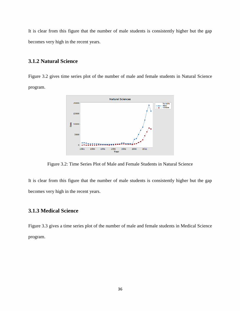
3.1.2 Natural Science

Figure 3.2 gives time series plot of the number of male and female students in Natural Science

program.

Figure 3.2: Time Series Plot of Male and Female Students in Natural Science



3.1.3 Medical Science

Figure 3.3 gives a time series plot of the number of male and female students in Medical Science

program.

37

Figure 3.3: Time Series Plot of Male and Female Students in Medical Science



3.1.4 Law

Figure 3.4 gives a time series plot of the number of male and female students in Law program.

Figure 3.4: Time Series Plot of Male and Female Students in Law



38

3.1.5 Humanities

Figure 3.5 gives a time series plot of the number of male and female students in Humanities

program.

Figure 3.5: Time Series Plot of Male and Female Students in Humanities

It is clear from this figure that the number of female students was higher initially. Then the gap

between male and female gets narrowed. However, in recent years the number of male students

gets increased and currently it is more than the female students.

3.1.6 Engineering

Figure 3.6 gives a time series plot of the number of male and female students in Engineering

program.

39

Figure 3.6: Time Series Plot of Male and Female Students in Engineering


becomes a rocket high in the recent years.

3.1.7 Education

Figure 3.7 gives a time series plot of the number of male and female students in Education

program.

Figure 3.7: Time Series Plot of Male and Female Students in Education

It is clear from this figure that the number of male students was higher before but the gap gets

narrowed and currently the number of female students has overtaken the number of male students.

40

3.1.8 Fine Arts

Figure 3.8 gives a time series plot of the number of male and female students in Fine Arts program.

Figure 3.8: Time Series Plot of Male and Female Students in Fine Arts

Probably this is the only program where the number of female students is consistently higher

than male students and the gap becomes higher in the recent years.

3.1.9 Agriculture

Figure 3.9 gives a time series plot of the number of male and female students in Agriculture

program.

Figure 3.9: Time Series Plot of Male and Female Students in Agriculture

41

Figure 3.9 shows that that the number of male students was much higher before. The gap narrowed

down gradually but the number of male students is consistently higher than the female students.

3.2 Tests for the Equality of Means between Male and Female

Students

In the previous section we have seen that in almost every program the number of male students is

higher than that of the female students. As we know graphs are very subjective here we test the

difference between mean of male and female students. Let us denote the number of male students

by X and the number of female students by Y. We are interested in testing the hypothesis .

against

:

Under 0H , the test statistic becomes

Assuming further normality and large sample sizes, the critical region for the test becomes

We test the equality of mean of male and female students for all nine programs and the results are

presented below. We present the average number of male and female students, z-value and its

corresponding p-value, whether the difference is significant or not, and if so, to which gender it is

biased. It is worth mentioning that * stands for significant at the 10% level, ** stands for significant

at the 5% level and *** stands for significant at the 1% level.

YXH :0

)/()/(22

mn

YXZ

YX

1H

mSnSzyx YX //||22

2/

YX

42

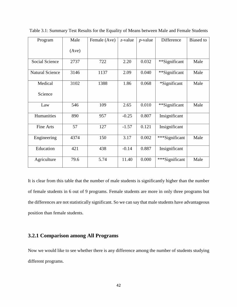
Table 3.1: Summary Test Results for the Equality of Means between Male and Female Students

Program Male

(Ave)

Female (Ave) z-value p-value Difference Biased to

Social Science 2737 722 2.20 0.032 **Significant Male

Natural Science 3146 1137 2.09 0.040 **Significant Male

Medical

Science

3102 1388 1.86 0.068 *Significant Male

Law 546 109 2.65 0.010 **Significant Male

Humanities 890 957 -0.25 0.807 Insignificant

Fine Arts 57 127 -1.57 0.121 Insignificant

Engineering 4374 150 3.17 0.002 ***Significant Male

Education 421 438 -0.14 0.887 Insignificant

Agriculture 79.6 5.74 11.40 0.000 ***Significant Male

It is clear from this table that the number of male students is significantly higher than the number

of female students in 6 out of 9 programs. Female students are more in only three programs but

the differences are not statistically significant. So we can say that male students have advantageous

position than female students.

3.2.1 Comparison among All Programs

Now we would like to see whether there is any difference among the number of students studying

different programs.

43

Table 3.2: Average Number of Students in Different Programs

Program Average Number of Students

Social Science 3459

Natural Science 4284

Medical Science 4490

Law 655

Humanities 1847

Fine Arts 184.6

Engineering 4524

Education 859

Agriculture 85.32

Socia

l Scie

nce

Natur

al Scie

nce

Medica

l Scie

nce

Law

Hum

anitie

s

Fine Arts

Engin

eerin

g

Educ

ation

Agricu

lture

35000

30000

25000

20000

15000

10000

5000

0

Dat

a

ure, Education, Engineering, Fine Arts, Humanities, Law, Medical Science, Natural Scie

Figure 3.10: Box Plot of Number of Students in Different Programs

44

The above table and the figure clearly shows differences in the average number of students, but

we also need to know whether this difference is statistically significant or not.

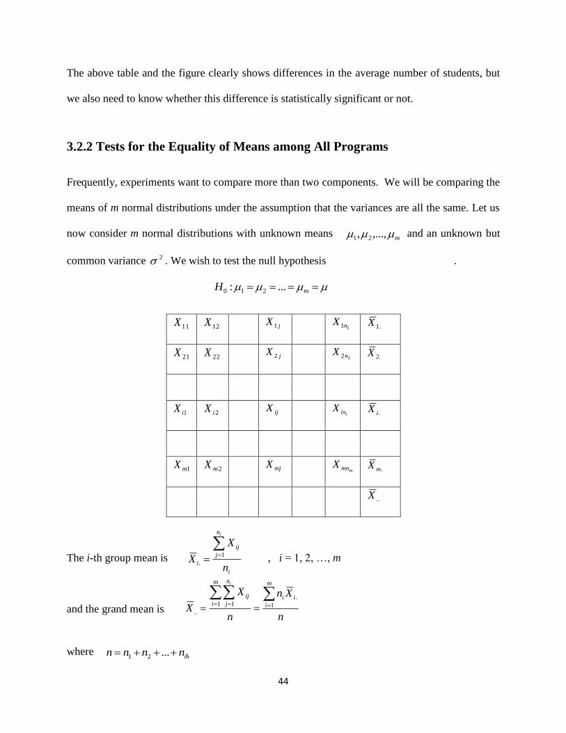
3.2.2 Tests for the Equality of Means among All Programs

Frequently, experiments want to compare more than two components. We will be comparing the

means of m normal distributions under the assumption that the variances are all the same. Let us

now consider m normal distributions with unknown means and an unknown but

common variance 2 . We wish to test the null hypothesis .

11X 12X jX1

11nX .1X

21X 22X jX 2

22nX .2X

1iX 2iX ijX

iinX .iX

1mX 2mX mjX

mmnX .mX

..X

The i-th group mean is , i = 1, 2, …, m

and the grand mean is

where .

m ,...,, 21

mH ...: 210

i

n

j

ij

in

X

X

i

1

.

n

Xn

n

X

X

m

i

ii

m

i

n

j

ij

i

1

.1 1

..

mnnnn ...21

45

To determine a critical region for a test of 0H , we partition the total sum of squares as

SS (TO) = =

Let = SS (Programs), the sum of squares among the different programs.

= SS (Error), the sum of squares within programs (often called the error

sum of squares).

It is easy to show that

, and

Hence, ~ and

Thus

The information used for the tests of the equality of several means is often summarized in an

analysis of variance (ANOVA) table.

Source Sum of Squares (SS) Degrees of Freedom Mean Squares (MS) F Ratio

Programs SS(P) m – 1 MS(P) = SS(P)/(m – 1) MS(P)/MS(E)

Error SS(E) n – m MS(E) = SS(E)/(n – m)

Total SS(T) n – 1

We would reject 0H if the observed value of F is too large. Thus the critical region is in the form

.

m

i

n

j

iiij

m

i

n

j

ij

ii

XXXXXX1 1

2

....

1 1

2

..

m

i

ii

m

i

n

j

iij XXnXXi

1

2

...

1 1

2

.

m

i

ii XXn1

2

...

m

i

n

j

iij

i

XX1 1

2

.

m

i

n

j

ij

i

nXX1 1

222

.. 1~/

1~/

2

2

.

i

i

n

X 1~ 2

2

1

2

.

i

n

j

iij

n

XXi

2

1

2

... /

m

i

ii XXn 12 m

mn

XXm

i

n

j

iij

i

2

2

1 1

2

.

~

mnmF

mn

m

,1~

/ErrorSS

1/ProgramSS

mnmFF ,1;

46

3.3 Comparison of the Individual Treatment Means

There are several methods by which we can compare treatment means.

3.3.1 The Least Significance Difference (Fisher’s LSD) Method

Suppose that following an analysis of variance F test where the null hypothesis is rejected, we

wish to test

jiH :0 for all i j.

This could be done by using the t statistic

t = ji

ji

nn

yy

/1/1EMS

..

The pair of means i and j would be declared significantly different if

jipNji nntyy /1/1EMS|| ),2/1(..

The quantity

LSD = jipN nnt /1/1EMS),2/1(

is called the least significant difference.

A design is called balanced when 1n = 2n = … = pn = n, and

LSD = nt pN 2EMS/),2/1(

47

3.3.2 Duncan’s Multiple Range Test

A widely used procedure for comparing all pairs of means is the multiple range test proposed by

Duncan. We first arrange the p treatment means in ascending order and compute the standard error

of each average as

hy nEMSs /.1

where

p

iih npn

1

/1/ .

If 1n = 2n = … = pn = n, we have hn = n, and hence nEMSsy /

.1

The significant ranges are calculated as

pNkrRk , .1ys , k = 2, 3, …, p

where the values of pNkr , is obtained from a table given by Duncan. Then the observed

differences between means are tested, beginning with the largest versus smallest and compared

with the least significant range pR . Next, the difference between the largest and the second

smallest is computed and compared with the least significant range 1pR . Finally, the difference

between the second largest and the smallest is computed and compared with the least significant

range 1pR . This process is continued until the differences of all possible p(p–1)/2 pairs of means

have been considered. If an observed difference is greater than the corresponding least significant

range, then we conclude that the pair of means in question is significantly different.

3.3.3 The Newman-Keuls Test

This test is similar to Duncan’s multiple range test, except that the critical difference between

means are calculated differently. Here we compute a set of critical values

48

K pNkqk , .1ys , k = 2, 3, …, p

where pNkq , is the upper percentage point of the Studentized range for groups of means

of size k and N – p error degrees of freedom.

The Studentized range is defined as

q = n

yy

/EMS

minmax

3.3.4 Tukey’s Test

Tukey proposed a multiple comparison procedure based on the Studentized range statistic. His

procedure requires the use of pNpq , to determine the critical value of all pairwise

comparisons, regardless of how many means are in the group. Thus, Tukey’s test declares two

means significantly different if the absolute value of their sample differences exceeds

T = pNpq , .1ys

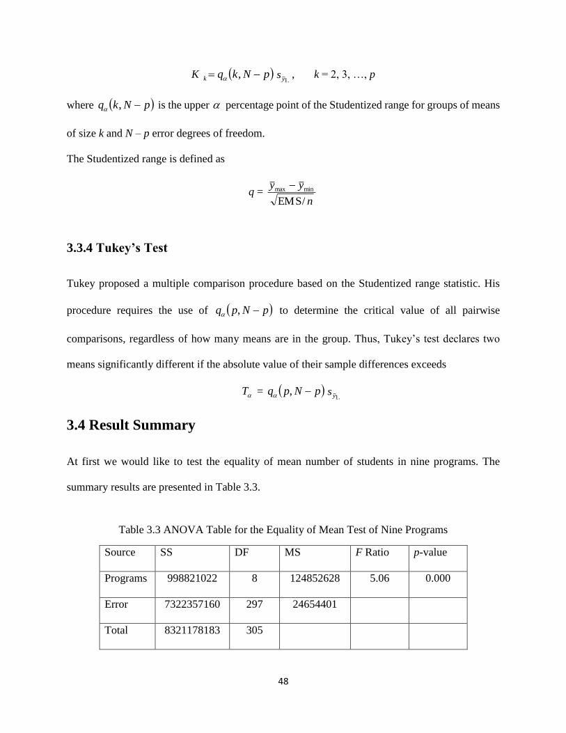
3.4 Result Summary

At first we would like to test the equality of mean number of students in nine programs. The

summary results are presented in Table 3.3.

Table 3.3 ANOVA Table for the Equality of Mean Test of Nine Programs

Source SS DF MS F Ratio p-value

Programs 998821022 8 124852628 5.06 0.000

Error 7322357160 297 24654401

Total 8321178183 305

49

Table 3.3 clearly shows that the programs effect is highly significant. So we must reject the

hypothesis of equal mean for the nine programs.

Now in search of which programs differ significantly from the other programs we report Tukey’s

test and Fisher’s LSD as they are very effective and readily available in MINITAB. Here we

present only the summary result the details result is presented in the Appendix.

Grouping Information Using Tukey Method

N Mean Grouping

Engineering 34 4524 A

Medical Science 34 4490 A

Natural Science 34 4284 A B

Social Science 34 3459 A B C

Humanities 34 1847 A B C

Education 34 859 A B C

Law 34 655 B C

Fine Arts 34 185 C

Agriculture 34 85 C

Tukey’s test shows that most of the Saudi Arabia students go abroad to study Engineering and

Medical Science and the least number of students study Agriculture and Fine Arts.

Grouping Information Using Fisher Method

N Mean Grouping



Natural Science 34 4284 A

Social Science 34 3459 A B

Humanities 34 1847 B C

Education 34 859 C

Law 34 655 C

Fine Arts 34 185 C

Agriculture 34 85 C

However, Fisher’s LSD shows most of the Saudi Arabia students go abroad to study Engineering,

Medical Science and Natural Science and the least popular programs are Agriculture, Fine Arts,

Law and Education.

50

CHAPTER 4

Modeling and Fitting of Data Using Regression

Diagnostics and Robust Regression

In this chapter at first we discuss classical regression method with diagnostics and then discuss

some robust methods that are commonly used in regression. We will employ all these things to

investigate which variables have significant impact on the number of Saudi Arabia students

studying abroad.

4.1 Classical Regression Analysis

Regression is probably the most popular and commonly used statistical method in all branches of

knowledge. It is a conceptually simple method for investigating functional relationships among

variables. The user of regression analysis attempts to discern the relationship between a dependent

(response) variable and one or more independent (explanatory/predictor/regressor) variables.

Regression can be used to predict the value of a response variable from knowledge of the values

of one or more explanatory variables.

We write the multiple regression model as

ikikiii XXXY ...22110 , i = 1, 2, …, n (4.1)

where Y is the dependent variable, the X’s are the independent variables, and is the error term.

Here we have a dependent variable and k explanatory variables excluding the intercept term. This

model is also called a k + 1 variable regression model.

51

The assumptions of the multiple regression model are quite similar to those of the two-variable

linear regression model:

The relationship between Y and X is linear. But no exact linear relationship exists between

two or more X’s.

The X’s are nonstochastic variables whose values are fixed.

The error has zero expected values: E( ) = 0

The error term has constant variance for all observations, i.e.,

E(2

i ) = 2 , i = 1, 2, …, n.

The random variables i are statistically independent. Thus,

E(ji ) = 0, for all i j.

The error term is normally distributed.

4.1.1 Estimation Technique

We can express the multiple regression model in matrix notation as:

Y = X + (4.2)

Where

Y =

ny

y

y

...

2

1

X =

knn

k

k

xx

xx

xx

...1

............

...1

...1

1

212

111

=

k

...

1

0

=

n

...

2

1

We obtain the OLS estimate of k unknown parameters 0 , 1 , …, k in such a way that the sum

of squares (SS)

n

ii

1

2 = XYXY

is minimized.

52

The value of that minimizes is given by the solution to

= 0

We get

= 2 YX – 2 XX = 0 = YXXX

1 (4.3)

We also have

V ( ) = 12 XX (4.4)

For this model, the residuals are

kikiiiii XXXYYY ˆ...ˆˆˆˆˆ22110 , i = 1, 2, …, n (4.5)

An unbiased and consistent estimate of 2 is )1/(ˆ1

22

knsn

ii . The estimated standard error

of j is jj

Vss 2ˆ

, where jV is the j-th diagonal element of 1

XX . When the errors are

normally distributed, then 1

ˆ

~ˆ

kn

j

jjt

s

4.1.2 Checking for Goodness of Fit

We can use the 2R statistic as a measure of goodness of fit for the multiple regression model. We

know that

2R = TSS

RSS = 1 –

TSS

ESS = 1 –

n

ii

n

ii

YY1

2

1

2

(4.6)

2R is the proportion of the total variation in Y explained by the regression of Y on X. It is easy to

show that 2R ranges in value between 0 and 1. But it is only a descriptive statistics. Roughly

53

speaking, we associate a high value of 2R (close to 1) with a good fit of the model by the regression

line and associate a low value of 2R (close to 0) with a poor fit. How large must 2R be for the

regression equation to be useful? That depends upon the area of application. If we could develop

a regression equation to predict the stock market, we would be ecstatic if 2R = 0.50. On the other

hand, if we were predicting death in road accident, we would want the prediction equation to have

strong predictive ability, since the consequences of poor prediction could be quite serious.

But the difficulty with 2R as a measure of goodness of fit is that it does not account for the number

of degrees of freedom. A natural solution is to use variances, not variations and that help to define

a corrected (adjusted)2R , defined as

2R = 1 – [Estimated V( ) / Estimated V(Y)]

Now

Estimated V( ) = )1/(ˆ1

22

knsn

ii

and

Estimated V(Y) =

n

ii YY

1

2/ (n – 1)

Thus the corrected 2R becomes

2R = 1 – 1

1ˆ

1

2

1

2

kn

n

YYn

ii

n

ii

= 1

111 2

kn

nR (4.7)

4.1.3 Tests of Regression Coefficients

We often like to establish that the explanatory variable X has a significant effect on Y, that the

coefficient of X (which is ) is significant. In this situation the null hypothesis is constructed in

54

way that makes its rejection possible. We begin with a null hypothesis, which usually states that a

certain effect is not present, i.e., = 0. We estimate and its standard error from the data and

compute the statistic

t =

ˆ

ˆ

s ~ 1knt (4.8)

4.2 Regression Diagnostics

Diagnostics are designed to find problems with the assumptions of any statistical procedure. In

diagnostic approach we estimate the parameters (in regression fit the model) by the classical

method (the OLS) and then see whether there is any violation of assumptions and/or irregularity

in the results regarding the six standard assumptions mentioned at the beginning of this section.

But among them the assumption of normality is the most important assumption.

4.2.1 Test for Normality

The normality assumption means the errors are distributed as normal. The simplest graphical

display for checking normality in regression analysis is the normal probability plot. This method

is based in the fact that if the ordered residuals are plotted against their cumulative probabilities

on normal probability paper, the resulting points should lie approximately on a straight line. An

excellent review of different analytical tests for normality is available in Imon (2003). A test based

on the correlation of true observations and the expectation of normalized order statistics is known

as the Shapiro – Wilk test. A test based on empirical distribution function is known as Anderson

– Darling test. It is often very useful to test whether a given data set approximates a normal

distribution. This can be evaluated informally by checking to see whether the mean and the median

55

are nearly equal, whether the skewness is approximately zero, and whether the kurtosis is close to

3. A more formal test for normality is given by the Jarque – Bera statistic:

JB = [n / 6] [22 )3( KS / 4] (4.9)

Imon (2003) suggests a slight adjustment to the JB statistic to make it more suitable for the

regression problems. His proposed statistic based on rescaled moments (RM) of ordinary least

squares residuals is defined as

RM = [n3c / 6] [

22 )3( KcS / 4] (4.10)

where c = n/(n – k), k is the number of independent variables in a regression model. Both the JB

and the RM statistic follow a chi square distribution with 2 degrees of freedom. If the values of

these statistics are greater than the critical value of the chi square, we reject the null hypothesis of

normality.

4.2.2 Outliers

In Statistics we often observe that the values of descriptive measures are often much influenced

by few extreme observations which are commonly known as outliers. According to Barnett and

Lewis (1993), ‘Observations which stand apart from the bulk of the data are called outliers.’

Different aspects of outliers with its consequences are discussed by Hadi, Imon and Werner (2009).

Hampel et al. (1986) claim that a routine data set typically contains about 1-10% outliers, and even

the highest quality data set cannot be guaranteed free of outliers. to Barnett and Lewis (1993)

commented ‘Any outliers, however, are always extreme values in the sample.’ But this statement

is not always true, especially in regression analysis.

56

In a regression problem, observations are judged as outliers on the basis of how unsuccessful the

fitted regression equation is in accommodating them and that is why observations corresponding

to excessively large residuals are treated as outliers.

Types of Outliers

X – Outlier: This is a point that is outlying in regard to the x–coordinate. In the literature an X–

outlier is more popularly known as a high leverage point.

Y – Outlier: This is a point that is outlying only because its y–coordinate is extreme.

X – and Y – Outlier: A point that is outlying in both x and y coordinates is known as x – and y –

outlier.

Residual Outlier: This is a point that has a large standardized (deletion) residual. Most of the

commonly used outlier detection methods are based on this approach where an observation is

judged as outlier on the basis of how unsuccessful the fitted regression equation is in

accommodating it.

Detection of Outliers

We often use the following three types of residuals for the identification of outliers.

Standardized residuals , i = 1, 2, …, n (4.11)

Studentized residuals , i = 1, 2, …, n (4.12)

Deletion Studentized (Externally Studentized or R-Student) residuals

, i = 1, 2, …, n (4.13)

ˆ

ˆT

iii

xyd

ii

T

iii

w

xyr

1ˆ

ˆ

iii

T

iii

w

xyt

1ˆ

ˆ

57

where is the OLS estimates of the mean squared error (MSE) based on a data set with the i-

th observation deleted.

As a thumb rule we call an observation outlier when its corresponding residual value exceeds 3 in

absolute value. A good review of recent outlier detection techniques in linear regression is

available in Imon (2008), and Hadi, Imon and Werner (2009).

4.2.3 Multicollinearity

One basic assumption of the multiple regression model is that there is no exact linear relationship

between any of the independent variables in the model. If such an exact linear relationship does

exist, we say that the independent variables are perfectly collinear or that perfect collinearity exists.

Multicollinearity arises when two or more variables (or combinations of variables) are highly

correlated with each other.

Effects of Multicollinearity

Wrong interpretation of the regression coefficients

Large variances and covariances for the OLS estimators of the regression parameters

Unduly large (in absolute value) estimates of the regression parameters

Indications of Multicollinearity

High Correlation Values

Calculate regression coefficients between all explanatory variables and test the maximum (in

absolute value) correlation coefficient by the statistic t = 2

1

2

ij

ij

r

nr

~ 2nt

2

ˆi

58

There is an evidence of multicollineatiy at the 5% level of significance if

|t| > 975.0,2nt

Large Variance Inflation Factor

We know that the variance of j is jV2 , where jV is the j-th diagonal element of 1

XX .

Consequently V( j ) is large, if jV is large. Hence

jV will be called the variance inflation

factor (VIF) of the explanatory variable jX . One or more large VIF’s indicate

multicollienarity.

Thumb rule: VIF < 5 No multicollinearity

5 VIF 10 Moderate multicollinearity

VIF > 10 Severe multicollinearity

Large Condition Number

A condition number is associated with the characteristic roots (eigen values) of the matrix XX .

The condition number of XX is defined as

min

max

A large condition number indicates the existence of multicollinearity.

Thumb rule: < 10 No multicollinearity

10 30 Moderate multicollinearity

> 30 Severe multicollinearity

Low Tolerance Value

Tolerance values are defined as inverse of VIF values. In other words, we can define

Tolerance value = 1/VIF

59

Since tolerance values are inverse of VIF’s, low tolerance values indicate multicollinearity

problem.

Thumb rule: VIF > 0.2 No multicollinearity

0.1 VIF 0.2 Moderate multicollinearity

VIF < 0.1 Severe multicollinearity

4.2.4 Variable Selection

In some applications theoretical considerations or prior experience can be helpful in selecting the

regressors to be used in the model. Building a regression model that includes only a subset of

available regressors involves two conflicting objectives.

1. We would like the model to include as many regressors as possible so that the information

content in these factors can influence the fitted value of the response.

2. We want the model to include as few regressors as possible because the variance of the fitted

response increases as the number of regressors increases. Also the more regressors there are in a

model, the greater the cost of data collection and model maintenance.

Finding an appropriate subset of regressors for the model is called the variable selection problem.

Graphical Methods

A number of graphical displays are used for variable selection. Here is a list of few of them

Added Variable Plot

Partial Residual (PR) plot (Ezekiel, 1924)

Component and Component-plus-residual (CCPR) plot (Wood, 1973)

60

Augmented Partial Residual (APR) plot (Mallows, 1986)

Conditional Expectation and Residual (CERES) plot (Cook, 1993)

Robust Added Variable Plot (Imon, 2003)

Model Selection Criteria

Minimum Residual Mean Square (RMS)

where SSE = is the residual sum of squares, n is the number of observations, k is the

number of explanatory variables.

Maximum R-Square

where SST is the total sum of squares.

Maximum Adjusted R-Square

Akaike Information Criterion

For a model with p = k + 1 predictors including the intercept, the Akaike information criterion

suggests to choose p for which the statistic

AIC (p) =

will be minimized. This statistic imposes a penalty for including insignificant variables.

1ˆ 2

kn

SSE

n

iii yy

1

2)ˆ(

,12

SST

SSER

n

ii yy

1

2)(

)1/(

)1/(12

nSST

knSSERa

n

p

n

n

ii

2ˆ

1ln

1

2

61

Mallows Cp

For a model with p predictors,

where is a good estimate of s2 (usually obtained from the full model). The above expression

can be reexpressed as

where 2

ˆp is the MSE from the sub model. It is straight forward to show that for the full model

pC = p. But here we search for a sub model where pC ≈ p for a value of p which is less than the

value of p for the full model.

Other Model Selection Criteria

Schwarz Criterion (SC)

Bayesian Information Criterion (BIC)

Final Prediction Error (FPE) or Prediction Criterion (PC)

Hannan-Quinn Criterion (HQC)

Variable Selection Methods

Forward Selection

Start with the empty model, then add the most significant variable (the one with the largest t-value

or smallest p-value). Repeat until all candidate variables to enter the model have insignificant

regression coefficients.

,)2(ˆ

)(2

npσ

YWIYC

T

p

2

,)2(

ˆ

ˆ

2

2

npσ

pnC

p

p

62

Backward Elimination

Start with the full model, then delete the least significant variable (the one with the smallest t-value

or largest p-value). Repeat until all regression coefficients in the model are significant.

Stepwise Method

This is a combination of forward selection and backward elimination methods.

4.3 Robust Regression

Robustness is now playing a key role in time series. According to Kadane (1984) ‘Robustness is a

fundamental issue for all statistical analyses; in fact it might be argued that robustness is the

subject of statistics.' The term robustness signifies insensitivity to small deviations from the

assumption. That means a robust procedure is nearly as efficient as the classical procedure when

classical assumptions hold strictly but is considerably more efficient over all when there is a small

departure from them. The main application of robust techniques in a time series problem is to try

to devise estimators that are not strongly affected by outliers or departures from the assumed

model. In time series, robust techniques grew up in parallel to diagnostics [see Hampel et al.

(1986)] and initially they were used to estimate parameters and to construct confidence intervals

in such a way that outliers or departures from the assumptions do not affect them. A large body of

literature is now available [Rousseuw and Leroy (1987), Maronna, Martin, and Yohai (2006), Hadi, Imon

and Werner (2009)] for robust techniques that are readily applicable in linear regression or in time series.

63

4.3.1. L – estimator

A first step toward a more robust time series estimator was the consideration of least absolute values

estimator (often referred to as L – estimator). In the OLS method, outliers may have a very large influence

since the estimated parameters are estimated by minimizing the sum of squared residuals

n

t

tu1

2

L estimates are then considered to be less sensitive since they are determined by minimizing the sum of

absolute residuals

n

t

tu1

||

The L estimator was first introduced by Edgeworth in 1887 who argued that the OLS method is over

influenced by outliers, but because of computational difficulties it was not popular and not much used

until quite recently. Sometimes we consider the L – estimator as a special case of pL -norm estimator in

the literature where the estimators are obtained by minimizing

n

t

p

tu1

||

The 1L -norm estimator is the OLS, while the 2L - norm estimator is the L – estimator. But unfortunately

a single erroneous observation (high leverage point) can still totally offset the L-estimator.

4.3.2. Least Median of Squares

Rousseeuw (1984) proposed Least Median of Squares (LMS) method which is a fitting technique less

sensitive to outliers than the OLS. In OLS, we estimate parameters by

Minimizing the sum of squared residuals

n

t

tu1

2

64

Which is obviously the same if we

Minimize the mean of squared residuals

n

t

tun 1

21.

Sample means are sensitive to outliers, but medians are not. Hence to make it less sensitive we can replace

the mean by a median to obtain median sum of squared residuals

MSR ( ) = Median {2

ˆtu } (4.14)

Then the LMS estimate of is the value that minimizes MSR ( ). Rousseeuw and Leroy (1987) have

shown that LMS estimates are very robust with respect to outliers and have the highest possible 50%

breakdown point.

4.3.3. Least Trimmed Squares

The least trimmed (sum of) squares (LTS) estimator is proposed by Rousseeuw (1984). In this method

we try to estimate in such a way that

LTS ( ) = minimize

h

t

tu1

2ˆ (4.15)

Here tu is the t-th ordered residual. For a trimming percentage of , Rousseeuw and Leroy (1987)

suggested choosing the number of observations h based on which the model is fitted as h = [n (1 – )]

+ 1. The advantage of using LTS over LMS is that, in the LMS we always fit the regression line based

on roughly 50% of the data, but in the LTS we can control the level of trimming. When we suspect that

the data contains nearly 10% outliers, the LTS with 10% trimming will certainly produce better result

than the LMS. We can increase the level of trimming if we suspect there are more outliers in the data.

65

4.3.4 Reweighted Least Squares

Another way to obtain a set of results based on a robust fit is the method of Reweighted Least

Squares (RLS) proposed by Rousseeuw and Leroy (1987). In this method, the parameters are

estimated by the LMS method and the outliers are identified. After that the final model is fitted by

the least squares without the potential outliers. Since this fitting does not involve any outliers this

method is claimed to be more appropriate for the majority of the observations. However, the

residuals of the deleted points are reestimated from the robust fit to produce a full set of residuals.

4.4 Regression Results

Here we employ regression method to understand which variables have significant impact on the

number of Saudi Arabia Students studying abroad. Budget in higher education can be an immediate

choice. Saud Arabia economy heavily relies on oil. So the two other variables one can consider

are oil price and oil revenue. We begin with a simple linear regression model with the number of

Saudi Arabia students studying abroad on the three explanatory variables one at a time.

Figure 4.1 gives a scatter plot of the total number of students versus budget in higher education.

We observe an upward and strong linear relationship between these two variables. The attached

MINITAB output shows that the value of 2R is 0.83 and the p-value corresponding to the variable

budget in higher education is highly significant (0.000).

66

2.0000E+111.5000E+111.0000E+115.0000E+100

100000

80000

60000

40000

20000

0

Budgei in HE

Tota

l No

. o

f S

tud

en

ts

Scatterplot of Total No. of Students vs Budgei in HE

Figure 4.1: Scatter Plot of the Total Number of Students vs Budget in Higher Education

Regression Analysis: Total No. of Students versus Budget in HE The regression equation is

Total No. of Students = - 5982 + 0.000000 Budget in HE

Predictor Coef SE Coef T P VIF

Constant -5982 3025 -1.98 0.057

Budget in HE 0.00000046 0.00000004 12.48 0.000 1.000

S = 12621.3 R-Sq = 83.0% R-Sq(adj) = 82.4%

Figure 4.2 gives a scatter plot of the total number of students versus budget in higher education.

We observe an upward and linear relationship between these two variables. The attached

MINITAB output shows that the value of 2R is 0.529 which is not great. This graph also shows

that probably there are few outliers in this data. So we think it will be a good idea to employ a

robust regression here. We fit the reweighted least squares (RLS) method to this data and the fitted

plot is presented in Figure 4.3.

67

100908070605040302010

100000

80000

60000

40000

20000

0

Oil Price

To

tal N

o.

of

Stu

de

nts

Scatterplot of Total No. of Students vs Oil Price

Figure 4.2: Scatter Plot of the Total Number of Students vs Oil Price

Regression Analysis: Total No. of Students versus Oil Price The regression equation is

Total No. of Students = - 19210 + 860 Oil Price


Constant -19210 7525 -2.55 0.016

Oil Price 860.3 143.6 5.99 0.000 1.000

S = 20985.0 R-Sq = 52.9% R-Sq(adj) = 51.4%

100908070605040302010

100000

80000

60000

40000

20000

0

Oil Price

No. o

f St

ude

nts

OLS

RLS

Total No. of Students

Variable

OLS and RLS Fit of Total No. of Students vs Oil Price

Figure 4.3: RLS and OLS Fit of the Total Number of Students vs Oil Price

68

Regression Analysis: Total No. of Students_1 versus Oil Price_1 The regression equation is

Total No. of Students_1 = - 29017 + 1363 Oil Price_1

Predictor Coef SE Coef T P

Constant -29017 2561 -11.33 0.000

Oil Price_1 1362.94 56.54 24.10 0.000

S = 6886.77 R-Sq = 96.2% R-Sq(adj) = 96.0%

We observe from Figure 4.3 that the robust RLS fit the data much better than the traditionally used

OLS fit. Now we observe an upward and very linear relationship between these two variables. The

attached MINITAB output shows that the value of 2R gets increased from 0.529 to 0.962 which

is a huge improvement. So we can say robust regression performs much better than the classical

regression method here.

120000010000008000006000004000002000000

100000

80000

60000

40000

20000

0

Oil Revenue

To

tal N

o.

of

Stu

de

nts

Scatterplot of Total No. of Students vs Oil Revenue

Figure 4.4: Scatter Plot of the Total Number of Students vs Oil Revenue

69

Figure 4.4 gives a scatter plot of the total number of students versus oil revenue. We observe an

upward and linear relationship between these two variables. The attached MINITAB output shows

that the value of 2R is 0.786 which is good.

Regression Analysis: Total No. of Students versus Oil Revenue The regression equation is

Total No. of Students = - 6054 + 0.0797 Oil Revenue


Constant -6054 3443 -1.76 0.088

Oil Revenue 0.079707 0.007362 10.83 0.000

S = 14154.7 R-Sq = 78.6% R-Sq(adj) = 77.9

Since each of the three explanatory variables shows a linear relationship with the total number of

students studying abroad, now we fit a multiple linear regression model.

Response variable: The total number of students studying abroad

Explanatory variables: Budget in higher education, Oil price, and Oil revenue.

Regression Analysis: Total No. of versus Budget in HE, Oil Revenue, Oil Price The regression equation is

Total No. of Students = - 18688 + 0.000000 Budget in HE - 0.0127 Oil Revenue

+ 417 Oil Price


Constant -18688 4476 -4.18 0.000

Budget in HE 0.00000042 0.00000008 5.23 0.000 6.812

Oil Revenue -0.01267 0.01897 -0.67 0.509 12.003

Oil Price 417.3 134.2 3.11 0.004 3.471

S = 10526.9 R-Sq = 88.9% R-Sq(adj) = 87.8%

The attached MINITAB output for multiple regression is quite confusing. Here the value of 2R is

0.889 which is good, but we observe that the effect of oil revenue is negative which completely

70

conflicts with our findings in Figure 4.4. It may be a clear case of wrong sign problem which is

caused by multicollinearity. We checked the VIF values and found the largest one as 12.003 which

shows that this model is severely affected by multicollinearity.

The above results suggest us that we cannot keep all the three explanatory variables in the model.

In quest of which of the explanatory variables should remain in the model we apply the forward

selection, the backward elimination and stepwise regression methods and the MINITAB results

are reported.

Stepwise Regression: Total No. of versus Oil Revenue, Budget in HE, ... Forward selection. Alpha-to-Enter: 0.05

Response is Total No. of Students on 3 predictors, with N = 34

Step 1 2

Constant -5982 -17088

Budget in HE 0.00000 0.00000

T-Value 12.48 9.92

P-Value 0.000 0.000

Oil Price 350

T-Value 3.98

P-Value 0.000

S 12621 10432

R-Sq 82.95 88.72

R-Sq(adj) 82.42 87.99

Mallows Cp 16.0 2.4

Stepwise Regression: Total No. of versus Oil Revenue, Budget in HE, ... Backward elimination. Alpha-to-Remove: 0.05


Step 1 2

Constant -18688 -17088

Oil Revenue -0.013

T-Value -0.67

P-Value 0.509

71

Budget in HE 0.00000 0.00000

T-Value 5.23 9.92

P-Value 0.000 0.000

Oil Price 417 350

T-Value 3.11 3.98

P-Value 0.004 0.000

S 10527 10432

R-Sq 88.88 88.72

R-Sq(adj) 87.77 87.99

Mallows Cp 4.0 2.4

Stepwise Regression: Total No. of versus Oil Revenue, Budget in HE, ... Alpha-to-Enter: 0.05 Alpha-to-Remove: 0.05


Step 1 2

Constant -5982 -17088

Budget in HE 0.00000 0.00000

T-Value 12.48 9.92

P-Value 0.000 0.000

Oil Price 350

T-Value 3.98

P-Value 0.000

S 12621 10432

R-Sq 82.95 88.72

R-Sq(adj) 82.42 87.99

Mallows Cp 16.0 2.4

All these three methods come up with exactly the same conclusion, i.e. the explanatory variables

that we should keep in our study are budget in higher education and oil price. Let us denote this as

Model A

Regression Analysis: Model A: Total No. of Stu versus Budget in HE, Oil Price The regression equation is

Total No. of Students = - 17088 + 0.000000 Budget in HE + 350 Oil Price


Constant -17088 3747 -4.56 0.000

Budget in HE 0.00000037 0.00000004 9.92 0.000 1.519

Oil Price 350.09 87.97 3.98 0.000 1.519

S = 10432.5 R-Sq = 88.7% R-Sq(adj) = 88.0%

72

The attached MINITAB output for Model A looks better now. Here the value of 2R is 0.887 which

is good, but more importantly we see that the effects of both of the explanatory variables are

positive and they are statistically significant.

3000020000100000-10000-20000-30000

99

95

90

80

70

60

50

40

30

20

10

5

1

Residuals

Pe

rce

nt

Mean 0

StDev 10111

N 34

AD 0.906

P-Value 0.019

Probability Plot of ResidualsNormal - 95% CI

Figure 4.5: Normal Probability Plot of the Residuals for Model A

But when we look at the normality plot of residuals as shown in Figure 4.5 we do not feel very

good about Model A. For this particular case the value of the Jarque-Bera test is 6.72 (p-value

0.0347) and the RM test is 8.37 (p-value 0.0152). So both of the tests reject the assumption of

normality of errors and thus the model looks questionable. As an alternative choice we fit the

same model by the robust reweighted least squares (RLS) method and we call it Model B.

Regression Analysis: Model B: Total No. of Stu versus Budget in HE_1, Oil Price_1 The regression equation is

Total No. of Students_1 = - 24848 + 0.000000 Budget in HE_1 + 992 Oil Price_1


Constant -24848 2647 -9.39 0.000

Budget in HE_1 0.00000016 0.00000005 2.91 0.008

Oil Price_1 991.7 136.8 7.25 0.000

S = 5984.88 R-Sq = 97.2% R-Sq(adj) = 97.0%

73

The attached MINITAB output shows that Model B produces even better fit in terms of 2R as its

value goes up to 0.972 from 0.887 when the OLS fit was done. Here the effects of both of the

explanatory variables are positive and they are statistically significant.

20000100000-10000-20000

99

95

90

80

70

60

50

40

30

20

10

5

1

RLS

Pe

rce

nt

Mean -7.56700E-12

StDev 5730

N 25

AD 0.532

P-Value 0.157

Probability Plot of RLSNormal - 95% CI

Figure 4.6: Normal Probability Plot of the Residuals for Model B

For model B, the normality plot of residuals as shown in Figure 4.6 look much better than what

we saw for Model A. For a confirmation we compute the Jarque-Bera and the RM values for Model

B. We see that the value of the Jarque-Bera test is 1.56 (p-value 0.4584) and the RM test is 1.69

(p-value 0.4296). So both of the tests now accept the assumption of normality of errors and thus

the model can be considered as a valid one.

In the previous chapter we have seen that most of the variables we consider here in our regression

model show exponential growth. So it may be a good idea to fit the model using a log

transformation on the response as suggested by Montgomery et al. (2013). This third model will

be denoted as Model C.

74

Regression Analysis: Model C: The regression equation is

Total No. of Students_2 = 7.44 + 0.000000 Budget in HE_2 + 0.0217 Oil Price_2


Constant 7.4370 0.1189 62.53 0.000

Budget in HE_2 0.00000000 0.00000000 10.12 0.000

Oil Price_2 0.021717 0.002792 7.78 0.000

S = 0.331114 R-Sq = 92.6% R-Sq(adj) = 92.1%

1.00.50.0-0.5-1.0

99

95

90

80

70

60

50

40

30

20

10

5

1

Residuals_1

Pe

rce

nt

Mean -4.44089E-15

StDev 0.3209

N 34

AD 0.459

P-Value 0.247

Probability Plot of Residuals_1Normal - 95% CI

Figure 4.7: Normal Probability Plot of the Residuals for Model C

The attached MINITAB output shows that Model C falls in between Model A and Model B in

terms of possessing better 2R . For this model the value of 2R is 0.926. But it was 0.972 for Model

B and 0.887 for Model A. Here the effects of both of the explanatory variables are positive and

they are statistically significant.

The normality plot of residuals for model C looks good as shown in Figure 4.7. Now we compute

the Jarque-Bera and the RM values for Model C. We see that the value of the Jarque-Bera test is

1.86 (p-value 0.3946) and the RM test is 1.97 (p-value 0.3734). So both of the tests now accept

the assumption of normality of errors and thus the model can be considered as a valid one.

75

4.5 Results Comparisons

In this section we summarize our above findings. To explain the number of students studying

abroad we began with three explanatory variables but this model failed the multicollinearity check.

After that we employed the variable selection procedure to select the best set of regressors. After

this selection was made we fit the data with three different models and the result summaries are

presented in Table 4.1.

Table 4.1: Regression Results Summary

Model 2R JB RM Normality

A: OLS 0.887 0.0347 0.0152 Rejected

B: RLS 0.972 0.4584 0.4296 Accepted

C: Exponential 0.926 0.3946 0.3734 Accepted

The above results suggest that the traditional least squares method performs worst among the three

models considered here. It not only possesses the lowest 2R , it fails the normality test as well.

Both the robust fit and the exponential model pass the normality test but we will put the robust

RLS ahead of the exponential model both in terms of possessing higher 2R and p-value in test of

normality.

76

CHAPTER 5

Cross Validation of Forecasts

In this chapter our main objective is to evaluate forecasts made by different regression methods

and models. We would employ the cross validation method for this purpose.

5.1 Evaluation of Forecasts by Cross Validation

Cross-validation is a technique for assessing how the results of a statistical analysis will generalize

to an independent data set. It is mainly used in settings where the goal is prediction, and one wants

to estimate how accurately a predictive model will perform in practice. One round of cross-

validation involves partitioning a sample of data into complementary subsets, performing the

analysis on one subset (called the training set), and validating the analysis on the other subset

(called the validation set or testing set). An excellent review of different type of cross validation

techniques is available in Izenman (2008). Picard and Cook (1984) developed all basic

fundamentals of applying cross validation technique in regression and time series.

According to Montgomery et al. (2013), three types of procedures are useful for validating a

regression or time series model.

(i) Analysis of the model coefficients and predicted values including comparisons with prior

experience, physical theory, and other analytical models or simulation results,

(ii) Collection of new data with which to investigate the model’s predictive performance,

77

(iii) Data splitting, that is, setting aside some of the original data and using these observations to

investigate the model’s predictive performance. Since we have a large number of data set, we

prefer the data splitting technique for cross-validation of the fitted model.

In order to find out the best prediction model we usually leave out say, l observations aside as

holdback period. The size of l is usually 10% to 20% of the original data. Suppose that we

tentatively select two models namely, A and B. We fit both the models using (T – l) set of

observations. Then we compute

l

t

AiA el

MSPE1

21 (5.1)

for model A and

l

t

BiB el

MSPE1

21 (5.2)

for model B. Several methods have been devised to determine whether one MSPE is statistically

different from the other. One such popular method of testing is the F-test approach, where F-

statistic is constructed as a ratio between the two MSPEs keeping the larger MSPE in the numerator

of the F-statistic. If the MSPE for model A is larger, this statistic takes the form:

B

A

MSPE

MSPEF (5.3)

This statistic follows an F distribution with (l , l) degrees of freedom under the null hypothesis of

equal forecasting performance. If the F-test is significant we will choose model B for this data

otherwise, we would conclude that there is a little bit difference in choosing between these two

models.

78

5.2 Cross Validation Results

In this section we employ the linear regression with the OLS and RLS methods and an exponential

model for cross validation. Since we have 34 years data, we will use the first 90% of our data (30

years) for fitting the model and information for the last 10% of observations (4 years) will be

forecasted by these three different methods.

Table 5.1: Original and Forecasted Values for 2011-2014

Year Original RLS OLS Exponential

2011 95991 89716.3 69734.2 70962

2012 86030 90866.4 78140.5 97382

2013 102302 95339.7 89855.8 136358

2014 90925 87741.9 89071.0 121570

102500100000975009500092500900008750085000

140000

130000

120000

110000

100000

90000

80000

70000

Original

Fore

ca

st

Original

RLS

OLS

Exponential

Variable

Scatterplot of Original vs RLS, OLS, Exponential Forecasts

Figure 5.1: Scatterplot of RLS, OLS, Exponential Forecasts vs Original Values

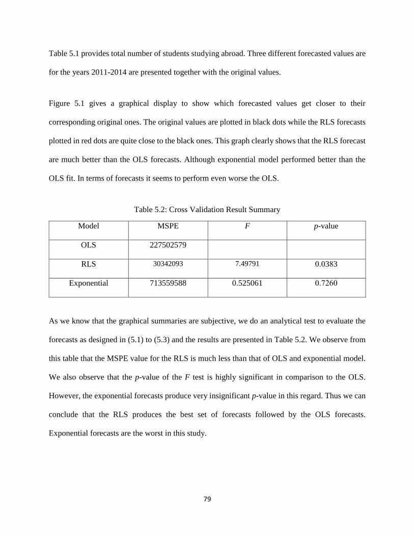
79

Table 5.1 provides total number of students studying abroad. Three different forecasted values are

for the years 2011-2014 are presented together with the original values.

Figure 5.1 gives a graphical display to show which forecasted values get closer to their

corresponding original ones. The original values are plotted in black dots while the RLS forecasts

plotted in red dots are quite close to the black ones. This graph clearly shows that the RLS forecast

are much better than the OLS forecasts. Although exponential model performed better than the

OLS fit. In terms of forecasts it seems to perform even worse the OLS.

Table 5.2: Cross Validation Result Summary

Model MSPE F p-value

OLS 227502579

RLS 30342093 7.49791 0.0383

Exponential 713559588 0.525061 0.7260

As we know that the graphical summaries are subjective, we do an analytical test to evaluate the

forecasts as designed in (5.1) to (5.3) and the results are presented in Table 5.2. We observe from

this table that the MSPE value for the RLS is much less than that of OLS and exponential model.

We also observe that the p-value of the F test is highly significant in comparison to the OLS.

However, the exponential forecasts produce very insignificant p-value in this regard. Thus we can

conclude that the RLS produces the best set of forecasts followed by the OLS forecasts.

Exponential forecasts are the worst in this study.

80

CHAPTER 6

Conclusions and Areas of Further Research

In this chapter we will summarize the findings of our research to draw some conclusions and

outline ideas for our future research.

6.1 Conclusions


studying abroad for higher education. We investigate both the overall trend and also trends of nine

individual programs. We observe that not a single variable fit linear trend model. All of them fit

either quadratic or exponential models. Then we investigate trends of some other variables such

as budget in higher education, oil price, and oil revenue which should influence the number of

students studying abroad. We observe similar trend for these variables as well.

We also observe that most of the Saudi Arabia students go abroad to study Engineering and

Medical Science and the least number of students study Agriculture and Fine Arts. We also found

that the number of male students is significantly higher than the number of female students in 6

out of 9 programs. Female students are more in only three programs but the differences are not

statistically significant. So we get an evidence of gender discrimination among the Saudi Arabia

students studying abroad.

In quest of which factors influence the number of students studying abroad we consider regression

analysis and the two variables that we found affect most are budget in higher education and oil

81

price. We also observe that commonly used least squares method have several limitations in this

case so we finally used the robust reweighted least squares to fit the data. To verify how good the

fit is, we did cross validation to generate forecasts for the last four years of data and we found that

the RLS fit produces much better forecasts than other methods.

Our findings cause a little bit concern about the future of the programs in which the Saudi Students

go abroad for higher studies. Since we see that oil price has a significant positive impact on the

number of students we suspect the recent fall in oil price might affect the programs adversely.

6.2 Areas of Further Research

Although our data sets are time series, we are not able to consider a variety of time series methods

due to time constraints. We only consider the deterministic models in fitting the data. In future we

would like to extend our research by considering stochastic ARIMA models. Volatility could be

an essential part of this data. We would like to consider ARCH/GARCH or ARFIMA/GARFIMA

models on these data in future.

82

References

1. Bowerman, B. L., O’Connell, R. T., and Koehler, A. B. (2005). Forecasting, Time

Series, and Regression: An Applied Approach, 4th Ed., Duxbury Publishing, Thomson

Books/Cole, New Jersey.

2. Hadi, A.S., Imon, A.H.M.R. and Werner, M. (2009). Detection of outliers, Wiley

Interdisciplinary Reviews: Computational Statistics, 1, pp. 57 – 70.

3. Hampel, F.R., Ronchetti, E.M., Rousseeuw, P.J. and Stahel, W. (1986). Robust

Statistics: The Approach Based on Influence Function, Wiley, New York.

4. Imon, A. H. M. R. (2003). Residuals from Deletion in Added Variable Plots, Journal of

Applied Statistics, 30, 841– 855.

5. Imon, A. H. M. R. (2003). Regression Residuals, Moments, and Their Use in Tests for

Normality, Communications in Statistics—Theory and Methods, 32, pp. 1021 – 1034.

6. Imon, A. H. M. R. (2008). Diagnostic Robust Approach of Outlier Detection in Regression,

Journal of Statistical Research, 42, 105 – 120.

7. Izenman, A.J. (2008), Modern Multivariate Statistical Techniques: Regression,

Classification, and Manifold Learning, Springer, New York.

8. Kadane, J.B. (1984). Robustness of Bayesian Analysis, Elsevier North-Holland,

Amsterdam.

9. Maronna, R.A., Martin, R.D. and Yohai, V.J. (2006), Robust Statistics: Theory and

Methods, Wiley, New York.

83

10 Montgomery, D., Jennings, C., and Kulachi, M. (2008), Introduction to Time Series

Analysis and Forecasting, Wiley, New York.

11. Montgomery, D., Peck, E., and Vining, G. (2013), An Introduction to Regression

Analysis, 5th Ed., Wiley, New York.

12. Pindyck, R. S. and Rubenfeld, D. L. (1998), Econometric Models and Economic

Forecasts, 4th Ed. Irwin/McGraw-Hill Boston.

13 Rousseeuw, P.J. (1984). Least Median of Squares Regression, Journal of the American

Statistical Association, 79, pp. 871 – 880.

14. Rousseeuw, P.J. and Leroy, A.M. (1987). Robust Regression and Outlier Detection, Wiley,

New York.

15. Rousseeuw, P.J. and Leroy, A.M. (1987). A Fast Algorithm for S-Regression Estimates,

Journal of Computational and Graphical Statistics, 15, pp. 414–427.

16. Saudi Arabian Moneytary Agency (SAMA).


17. Saudi Arabia Cultural Mission to the U.S.

http://www.sacm.org/ArabicSACM/pdf/Posters_Sacm_schlorship.pdf

19. The Ministry of Education

https://www.mohe.gov.sa/ar/Ministry/Deputy-Ministry-for-Planning-and-

Information-affairs/HESC/Ehsaat/Pages/default.aspx

20. The Ministry of Education


http://www.stat.ualberta.ca/~wiens/stat578/papers/Salibian-Barrera%20&%20Yohai.pdf


http://www.sacm.org/ArabicSACM/pdf/Posters_Sacm_schlorship.pdf




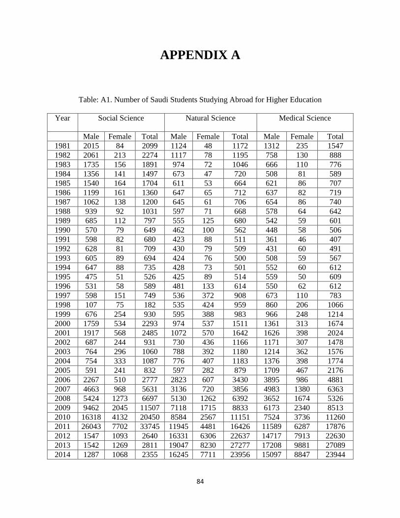
84

APPENDIX A

Table: A1. Number of Saudi Students Studying Abroad for Higher Education

Year Social Science Natural Science Medical Science

Male Female Total Male Female Total Male Female Total

1981 2015 84 2099 1124 48 1172 1312 235 1547

1982 2061 213 2274 1117 78 1195 758 130 888

1983 1735 156 1891 974 72 1046 666 110 776

1984 1356 141 1497 673 47 720 508 81 589

1985 1540 164 1704 611 53 664 621 86 707

1986 1199 161 1360 647 65 712 637 82 719

1987 1062 138 1200 645 61 706 654 86 740

1988 939 92 1031 597 71 668 578 64 642

1989 685 112 797 555 125 680 542 59 601

1990 570 79 649 462 100 562 448 58 506

1991 598 82 680 423 88 511 361 46 407

1992 628 81 709 430 79 509 431 60 491

1993 605 89 694 424 76 500 508 59 567

1994 647 88 735 428 73 501 552 60 612

1995 475 51 526 425 89 514 559 50 609

1996 531 58 589 481 133 614 550 62 612

1997 598 151 749 536 372 908 673 110 783

1998 107 75 182 535 424 959 860 206 1066

1999 676 254 930 595 388 983 966 248 1214

2000 1759 534 2293 974 537 1511 1361 313 1674

2001 1917 568 2485 1072 570 1642 1626 398 2024

2002 687 244 931 730 436 1166 1171 307 1478

2003 764 296 1060 788 392 1180 1214 362 1576

2004 754 333 1087 776 407 1183 1376 398 1774

2005 591 241 832 597 282 879 1709 467 2176

2006 2267 510 2777 2823 607 3430 3895 986 4881

2007 4663 968 5631 3136 720 3856 4983 1380 6363

2008 5424 1273 6697 5130 1262 6392 3652 1674 5326

2009 9462 2045 11507 7118 1715 8833 6173 2340 8513

2010 16318 4132 20450 8584 2567 11151 7524 3736 11260

2011 26043 7702 33745 11945 4481 16426 11589 6287 17876

2012 1547 1093 2640 16331 6306 22637 14717 7913 22630

2013 1542 1269 2811 19047 8230 27277 17208 9881 27089

2014 1287 1068 2355 16245 7711 23956 15097 8847 23944

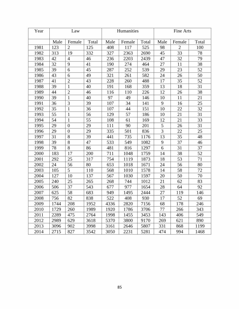
85

Year Law Humanities Fine Arts


1981 123 2 125 408 117 525 98 2 100

1982 313 19 332 327 2363 2690 45 33 78

1983 42 4 46 236 2203 2439 47 32 79

1984 32 9 41 190 274 464 27 11 38

1985 39 6 45 287 252 539 29 23 52

1986 43 6 49 321 261 582 24 26 50

1987 41 2 43 228 260 488 17 35 52

1988 39 1 40 191 168 359 13 18 31

1989 44 2 46 116 110 226 12 26 38

1990 39 1 40 97 49 146 10 11 21

1991 36 3 39 107 34 141 9 16 25

1992 35 1 36 107 44 151 10 22 32

1993 55 1 56 129 57 186 10 21 31

1994 54 1 55 108 61 169 12 21 33

1995 29 0 29 111 90 201 5 26 31

1996 29 0 29 335 501 836 3 22 25

1997 31 8 39 441 735 1176 13 35 48

1998 39 8 47 533 549 1082 9 37 46

1999 78 8 86 481 816 1297 6 31 37

2000 183 17 200 711 1048 1759 14 38 52

2001 292 25 317 754 1119 1873 18 53 71

2002 24 56 80 653 1018 1671 24 56 80

2003 105 5 110 568 1010 1578 14 58 72

2004 127 10 137 567 1030 1597 20 50 70

2005 240 25 265 268 744 1012 21 62 83

2006 506 37 543 677 977 1654 28 64 92

2007 625 58 683 949 1495 2444 27 119 146

2008 756 82 838 522 408 930 17 52 69

2009 1744 208 1952 4336 2820 7156 68 178 246

2010 1729 260 1989 1920 1786 3706 77 266 343

2011 2289 475 2764 1998 1455 3453 143 406 549

2012 2989 629 3618 5370 3800 9170 269 621 890

2013 3096 902 3998 3161 2646 5807 331 868 1199

2014 2715 827 3542 3050 2231 5281 474 994 1468

86

Year Engineering Education Agriculture


1981 1490 20 1510 382 25 407 219 1 220

1982 1137 14 1151 516 212 728 176 4 180

1983 1026 68 1094 514 265 779 138 3 141

1984 849 12 861 339 202 541 107 2 109

1985 737 9 746 473 309 782 99 3 102

1986 537 17 554 296 344 640 81 4 85

1987 499 6 505 174 351 525 95 3 98

1988 449 10 459 157 192 349 82 0 82

1989 451 9 460 148 106 254 82 1 83

1990 428 10 438 120 68 188 52 1 53

1991 467 18 485 123 87 210 49 1 50

1992 362 3 365 120 93 213 50 0 50

1993 407 2 409 104 93 197 55 1 56

1994 411 6 417 109 88 197 62 1 63

1995 419 37 456 62 60 122 61 2 63

1996 544 15 559 74 55 129 54 2 56

1997 1123 34 1157 118 88 206 66 2 68

1998 1435 100 1535 107 75 182 58 6 64

1999 542 46 588 228 353 581 82 3 85

2000 498 43 541 459 631 1090 82 4 86

2001 516 44 560 458 560 1018 83 8 91

2002 681 88 769 193 311 504 79 4 83

2003 2711 162 2873 176 276 452 74 10 84

2004 5481 292 5773 177 167 344 54 13 67

2005 5080 130 5210 171 224 395 34 5 39

2006 6665 317 6982 300 323 623 81 15 96

2007 10647 360 11007 2144 1019 3163 80 31 111

2008 18104 692 18796 319 216 535 29 0 29

2009 21461 672 22133 1254 710 1964 44 0 44

2010 30164 968 31132 610 716 1326 74 2 76

2011 26255 860 27115 955 1341 2296 74 12 86

2012 1490 20 1510 863 1342 2205 88 19 107

2013 1137 14 1151 1016 1867 2883 88 18 106

2014 1026 68 1094 1059 2117 3176 74 14 88

87

Table: A2. Saudi Arabia Oil Revenue, Oil Price and Budget in Higher Education

Year Oil Revenue Budget in HE Oil Price

1981 328594 2.76845E+06 77.80

1982 186006 9.35426E+06 74.58

1983 145123 1.03608E+07 68.43

1984 121348 9.30524E+06 69.36

1985 88425 1.10786E+07 67.16

1986 42464 7.13496E+09 26.21

1987 67405 6.00293E+09 28.38

1988 48400 6.15068E+09 20.45

1989 75900 5.73860E+09 25.20

1990 96800 5.75337E+09 28.40

1991 149497 6.09730E+09 23.50

1992 128790 3.18550E+10 22.64

1993 105976 3.41000E+10 20.52

1994 95505 3.51000E+10 19.31

1995 105728 2.69120E+10 19.24

1996 135982 2.76267E+10 23.07

1997 159985 4.17000E+10 23.04

1998 79998 4.31000E+10 15.08

1999 104447 4.41000E+10 21.60

2000 214424 4.92840E+10 35.64

2001 183915 5.43000E+10 31.14

2002 166100 4.70370E+10 31.27

2003 231000 6.75000E+10 30.92

2004 330000 6.36500E+10 35.14

2005 504540 7.01000E+10 50.21

2006 604470 8.73000E+10 59.94

2007 562186 9.67000E+10 62.59

2008 983369 1.05000E+11 80.38

2009 434420 1.22100E+11 53.89

2010 670265 1.37600E+11 68.60

2011 1034360 1.50000E+11 88.79

2012 1144818 1.68600E+11 93.06

2013 1035046 2.04000E+11 88.95

2014 913346 2.10000E+11 80.34

88

APPENDIX B

One-way ANOVA: Agriculture, Education, Engineering, Fine Arts, Humanities, ... Source DF SS MS F P

Factor 8 998821022 124852628 5.06 0.000

Error 297 7322357160 24654401

Total 305 8321178183

S = 4965 R-Sq = 12.00% R-Sq(adj) = 9.63%

Individual 95% CIs For Mean Based on

Pooled StDev

Level N Mean StDev --------+---------+---------+---------+-

Agriculture 34 85 38 (-------*--------)

Education 34 859 895 (-------*--------)

Engineering 34 4524 8019 (--------*-------)

Fine Arts 34 185 340 (-------*-------)

Humanities 34 1847 2142 (-------*--------)

Law 34 655 1159 (-------*--------)

Medical Science 34 4490 7337 (-------*--------)

Natural Science 34 4284 7319 (-------*--------)

Social Science 34 3459 6584 (-------*--------)

--------+---------+---------+---------+-

0 2000 4000 6000

Pooled StDev = 4965

One-way ANOVA: Agriculture, Education, Engineering, Fine Arts, Humanities, ... Source DF SS MS F P

Factor 8 998821022 124852628 5.06 0.000

Error 297 7322357160 24654401

Total 305 8321178183

S = 4965 R-Sq = 12.00% R-Sq(adj) = 9.63%

Individual 95% CIs For Mean Based on

Pooled StDev

Level N Mean StDev --------+---------+---------+---------+-

Agriculture 34 85 38 (-------*--------)

Education 34 859 895 (-------*--------)

Engineering 34 4524 8019 (--------*-------)

Fine Arts 34 185 340 (-------*-------)

Humanities 34 1847 2142 (-------*--------)

Law 34 655 1159 (-------*--------)

Medical Science 34 4490 7337 (-------*--------)

Natural Science 34 4284 7319 (-------*--------)

Social Science 34 3459 6584 (-------*--------)

--------+---------+---------+---------+-

0 2000 4000 6000

Pooled StDev = 4965

Grouping Information Using Tukey Method

89

N Mean Grouping



Natural Science 34 4284 A B

Social Science 34 3459 A B C

Humanities 34 1847 A B C

Education 34 859 A B C

Law 34 655 B C

Fine Arts 34 185 C

Agriculture 34 85 C

Means that do not share a letter are significantly different.

Tukey 95% Simultaneous Confidence Intervals

All Pairwise Comparisons

Individual confidence level = 99.79%

Agriculture subtracted from:

Lower Center Upper ------+---------+---------+---------+---

Education -2965 774 4512 (-------*------)

Engineering 700 4439 8177 (-------*------)

Fine Arts -3639 99 3838 (------*-------)

Humanities -1977 1761 5500 (-------*------)

Law -3169 569 4308 (------*-------)

Medical Science 666 4405 8143 (-------*------)

Natural Science 460 4198 7937 (------*-------)

Social Science -365 3373 7112 (-------*------)

------+---------+---------+---------+---

-5000 0 5000 10000

Education subtracted from:


Engineering -73 3665 7403 (------*-------)

Fine Arts -4413 -674 3064 (-------*------)

Humanities -2751 988 4726 (-------*------)

Law -3943 -204 3534 (-------*------)

Medical Science -107 3631 7369 (------*-------)

Natural Science -314 3425 7163 (-------*------)

Social Science -1138 2600 6338 (------*-------)

------+---------+---------+---------+---

-5000 0 5000 10000

Engineering subtracted from:


Fine Arts -8078 -4339 -601 (------*-------)

Humanities -6415 -2677 1061 (-------*------)

Law -7607 -3869 -131 (------*-------)

Medical Science -3772 -34 3704 (-------*------)

Natural Science -3979 -240 3498 (-------*------)

Social Science -4803 -1065 2673 (-------*------)

------+---------+---------+---------+---

-5000 0 5000 10000

90

Fine Arts subtracted from:


Humanities -2076 1662 5400 (------*-------)

Law -3268 470 4208 (-------*------)

Medical Science 567 4305 8044 (-------*------)

Natural Science 361 4099 7837 (------*-------)

Social Science -464 3274 7012 (-------*------)

------+---------+---------+---------+---

-5000 0 5000 10000

Humanities subtracted from:


Law -4930 -1192 2546 (-------*------)

Medical Science -1095 2643 6382 (------*-------)

Natural Science -1301 2437 6175 (-------*------)

Social Science -2126 1612 5350 (------*-------)

------+---------+---------+---------+---

-5000 0 5000 10000

Law subtracted from:


Medical Science 97 3835 7574 (-------*------)

Natural Science -109 3629 7367 (------*-------)

Social Science -934 2804 6542 (-------*------)

------+---------+---------+---------+---

-5000 0 5000 10000

Medical Science subtracted from:


Natural Science -3945 -206 3532 (-------*------)

Social Science -4770 -1031 2707 (-------*------)

------+---------+---------+---------+---

-5000 0 5000 10000

Natural Science subtracted from:


Social Science -4563 -825 2913 (------*-------)

------+---------+---------+---------+---

-5000 0 5000 10000

Grouping Information Using Fisher Method

N Mean Grouping



Natural Science 34 4284 A

Social Science 34 3459 A B

Humanities 34 1847 B C

Education 34 859 C

Law 34 655 C

Fine Arts 34 185 C

Agriculture 34 85 C

91

Means that do not share a letter are significantly different.

Fisher 95% Individual Confidence Intervals

All Pairwise Comparisons

Simultaneous confidence level = 43.41%

Agriculture subtracted from:

Lower Center Upper ---------+---------+---------+---------+

Education -1596 774 3144 (------*------)

Engineering 2069 4439 6809 (------*-----)

Fine Arts -2271 99 2469 (-----*------)

Humanities -609 1761 4131 (------*------)

Law -1801 569 2939 (------*-----)

Medical Science 2035 4405 6775 (------*-----)

Natural Science 1828 4198 6568 (------*------)

Social Science 1003 3373 5743 (------*-----)

---------+---------+---------+---------+

-3500 0 3500 7000

Education subtracted from:


Engineering 1295 3665 6035 (-----*------)

Fine Arts -3044 -674 1696 (------*------)

Humanities -1382 988 3358 (------*------)

Law -2574 -204 2166 (-----*------)

Medical Science 1261 3631 6001 (-----*------)

Natural Science 1055 3425 5795 (------*------)

Social Science 230 2600 4970 (-----*------)

---------+---------+---------+---------+

-3500 0 3500 7000

Engineering subtracted from:


Fine Arts -6709 -4339 -1969 (------*-----)

Humanities -5047 -2677 -307 (-----*------)

Law -6239 -3869 -1499 (------*------)

Medical Science -2404 -34 2336 (------*------)

Natural Science -2610 -240 2130 (-----*------)

Social Science -3435 -1065 1305 (------*------)

---------+---------+---------+---------+

-3500 0 3500 7000

Fine Arts subtracted from:


Humanities -708 1662 4032 (------*------)

Law -1900 470 2840 (-----*------)

Medical Science 1935 4305 6675 (-----*------)

Natural Science 1729 4099 6469 (------*-----)

Social Science 904 3274 5644 (-----*------)

---------+---------+---------+---------+

-3500 0 3500 7000

92

Humanities subtracted from:


Law -3562 -1192 1178 (------*-----)

Medical Science 273 2643 5013 (------*-----)

Natural Science 67 2437 4807 (------*------)

Social Science -758 1612 3982 (------*-----)

---------+---------+---------+---------+

-3500 0 3500 7000

Law subtracted from:


Medical Science 1465 3835 6205 (------*------)

Natural Science 1259 3629 5999 (-----*------)

Social Science 434 2804 5174 (------*------)

---------+---------+---------+---------+

-3500 0 3500 7000

Medical Science subtracted from:


Natural Science -2576 -206 2164 (-----*------)

Social Science -3401 -1031 1339 (------*------)

---------+---------+---------+---------+

-3500 0 3500 7000

Natural Science subtracted from:


Social Science -3195 -825 1545 (------*-----)

---------+---------+---------+---------+

-3500 0 3500 7000

Documents

Trend of Saudi Arabia Students Taking Higher Education Abroad