Trend Filtering Methods for Momentum Strategiesthierry-roncalli.com/download/lwp-tf.pdf · 1. the trend following strategy, ... in trading strategies. ... Trend Filtering Methods

Trend Filtering Methodsfor Momentum Strategies∗

Benjamin BruderResearch & Development

Lyxor Asset Management, [email protected]

Tung-Lam DaoResearch & Development


Jean-Charles RichardResearch & Development


Thierry RoncalliResearch & Development


December 2011

Abstract

This paper studies trend filtering methods. These methods are widely used in mo-mentum strategies, which correspond to an investment style based only on the historyof past prices. For example, the CTA strategy used by hedge funds is one of thebest-known momentum strategies. In this paper, we review the different econometricestimators to extract a trend of a time series. We distinguish between linear and non-linear models as well as univariate and multivariate filtering. For each approach, weprovide a comprehensive presentation, an overview of its advantages and disadvantagesand an application to the S&P 500 index. We also consider the calibration problem ofthese filters. We illustrate the two main solutions, the first based on prediction error,and the second using a benchmark estimator. We conclude the paper by listing someissues to consider when implementing a momentum strategy.

Keywords: Momentum strategy, trend following, moving average, filtering, trend extrac-tion.

JEL classification: G11, G17, C63.

1 IntroductionThe efficient market hypothesis tells us that financial asset prices fully reflect all availableinformation (Fama, 1970). One consequence of this theory is that future returns are notpredictable. Nevertheless, since the beginning of the nineties, a large body of academicresearch has rejected this assumption. One of the arguments is that risk premiums are timevarying and depend on the business cycle (Cochrane, 2001). In this framework, returnson financial assets are related to some slow-moving economic variables that exhibit cyclicalpatterns in accordance with the business cycle. Another argument is that some agents are

∗We are grateful to Guillaume Jamet and Hoang-Phong Nguyen for their helpful comments.

Trend Filtering Methods for Momentum Strategies

not fully rational, meaning that prices may underreact in the short run but overreact at longhorizons (Hong and Stein, 1997). This phenomenon may be easily explained by the theoryof behavioural finance (Barberis and Thaler, 2002).

Based on these two arguments, it is now commonly accepted that prices may exhibittrends or cycles. In some sense, these arguments chime with the Dow theory (Brown et al.,1998), which is one of the first momentum strategies. A momentum strategy is an investmentstyle based only on the history of past prices (Chan et al., 1996). We generally distinguishbetween two types of momentum strategy:

1. the trend following strategy, which consists of buying (or selling) an asset if the esti-mated price trend is positive (or negative);

2. the contrarian (or mean-reverting) strategy, which consists of selling (or buying) anasset if the estimated price trend is positive (or negative).

Contrarian strategies are clearly the opposite of trend following strategies. One of the tasksinvolved in these strategies is to estimate the trend, excepted when based on mean-revertingprocesses (see D’Aspremont, 2011). In this paper, we provide a survey of the differenttrend filtering methods. However, trend filtering is just one of the difficulties in building amomentum strategy. The complete process of constructing a momentum strategy is highlycomplex, especially as regards transforming past trends into exposures – an important factorthat is beyond the scope of this paper.

The paper is organized as follows. Section two presents a survey of the different econo-metric trend estimators. In particular, we distinguish between methods based on linearfiltering and nonlinear filtering. In section three, we consider some issues that arise whentrend filtering is applied in practice. We also propose some methods for calibrating trendfiltering models and highlight the problem of estimator variance. Section four offers someconcluding remarks.

2 A review of econometric estimators for trend filtering

Trend filtering (or trend detection) is a major task of time series analysis from both amathematical and financial viewpoint. The trend of a time series is considered to be thecomponent containing the global change, which contrasts with local changes due to noise.The trend filtering procedure concerns not only the problem of denoising; it must alsotake into account the dynamics of the underlying process. This explains why mathematicalapproaches to trend extraction have a long history, and why this subject is still of greatinterest to the scientific community1. From an investment perspective, trend filtering isfundamental to most momentum strategies developed in asset management and hedge fundssectors in order to improve performance and limit portfolio risks.

2.1 The trend-cycle model

In economics, trend-cycle decomposition plays an important role by identifying the perma-nent and transitory stochastic components in a non-stationary time series. Generally, thepermanent component can be interpreted as a trend, whereas the transitory component may

1See Alexandrov et al. (2008).

2


be a noise or a stochastic cycle. Let yt be a stochastic process. We assume that yt is thesum of two different unobservable parts:

yt = xt + εt

where xt represents the trend and εt is a stochastic (or noise) process. There is no precisedefinition for trend, but it is generally accepted to be a smooth function representing long-term movements:

“ [...] the essential idea of trend is that it shall be smooth.” (Kendall, 1973).

It means that changes in the trend xt must be smaller than those of the process yt. From astatistical standpoint, it implies that the volatility of yt − yt−1 is higher than the volatilityof xt − xt−1:

σ (yt − yt−1) ≫ σ (xt − xt−1)

One of the major problems in financial econometrics is the estimation of xt. This is thesubject of signal extraction and filtering (Pollock, 2009).

Finite moving average filtering for trend estimation has a long history. It has been usedin actuarial science since the beginning of the twentieth century2. But the modern theory ofsignal filtering has its origins in the Second World War and was formulated independentlyby Norbert Wiener (1941) and Andrei Kolmogorov (1941) in two different ways. Wienerworked principally in the frequency domain whereas Kolmogorov considered a time-domainapproach. This theory was extensively developed in the fifties and sixties by mathematiciansand statisticians such as Hermann Wold, Peter Whittle, Rudolf Kalman, Maurice Priestley,George Box, etc. In economics, the problem of trend filtering is not a recent one, and maydate back to the seminal article of Muth (1960). It was extensively studied in the eighties andnineties in the literature on business cycles, which led to a vast body of empirical researchbeing carried out in this area3. However, it is in climatology that trend filtering is mostextensively studied nowadays. Another important point is that the development of filteringtechniques has evolved according to the development of computational power and the ITindustry. The Savitzky-Golay smoothing procedure may appear very basic today though itwas revolutionary4 when it was published in 1964.

In what follows, we review the class of filtering techniques that is generally used toestimate a trend. Moving average filters play an important role in finance. As they are veryintuitive and easy to implement, they undoubtedly represent the model most commonly usedin trading strategies. The moving average technique belongs to the class of linear filters,which share a lot of common properties. After studying this class of filters, we considersome nonlinear filtering techniques, which may be well suited to solving financial problems.

2.2 Linear filtering2.2.1 The convolution representation

We denote by y = . . . , y−2, y−1, y0, y1, y2, . . . the ordered sequence of observations of theprocess yt. Let xt be the estimator of the underlying trend xt which is by definition an

2See, in particular, the works of Henderson (1916), Whittaker (1923) and Macaulay (1931).3See for example Cleveland and Tiao (1976), Beveridge and Nelson (1981), Harvey (1991) or Hodrick and

Prescott (1997).4The paper of Savitzky and Golay (1964) is still considered by the Analytical Chemistry journal to be

one of its 10 seminal papers.

3


unobservable process. A filtering procedure consists of applying a filter L to the data y:

x = L (y)

with x = . . . , x−2, x−1, x0, x1, x2, . . .. When the filter is linear, we have x = Ly with thenormalisation condition 1 = L1. If we assume that the signal yt is observed at regulardates5, we obtain:

xt =∞∑

i=−∞Lt,t−iyt−i (1)

We deduce that linear filtering may be viewed as a convolution. The previous filter may notbe of much use, however, because it uses future values of yt. As a result, we generally imposesome restriction on the coefficients Lt,t−i in order to use only past and present values of thesignal. In this case, we say that the filter is causal. Moreover, if we restrict our study totime invariant filters, the equation (1) becomes a simple convolution of the observed signalyt with a window function Li:

xt =n−1∑i=0

Liyt−i (2)

With this notation, a linear filter is characterised by a window kernel Li and its support.The kernel defines the type of filtering, whereas the support defines the range of the filter.For instance, if we take a square window on a compact support [0, T ] with T = n∆ thewidth of the averaging window, we obtain the well-known moving average filter:

Li =1

n1 i < n

We finish this description by considering the lag representation:

xt =n−1∑i=0

LiLiyt

with the lag operator L satisfying Lyt = yt−1.

2.2.2 Measuring the trend and its derivative

We discuss here how to use linear filtering to measure the trend of an asset price and itsderivative. Let St be the asset price which follows the dynamics of the Black-Scholes model:

dSt

St= µt dt+ σt dWt

where µt is the drift, σt is the volatility and Wt is a standard Brownian motion. Theasset price St is observed in a series of discrete dates t0, . . . , tn. Within this model, theappropriate signal to be filtered is the logarithm of the price yt = lnSt but not the priceitself. Let Rt = lnSt − lnSt−1 represent the realised return at time t over a unit period. Ifµt and σt are known, we have:

Rt =

(µt −

1

2σ2t

)∆+ σt

√∆ηt

5We have ti+1 − ti = ∆.

4


where ηt is a standard Gaussian white noise. The filtered trend can be extracted using thefollowing equation:

xt =

n−1∑i=0

Liyt−i

and the estimator of µt is6:

µt ≃1

∆

n−1∑i=0

LiRt−i

We can also obtain the same result by applying the filter directly to the signal and definingthe derivative of the window function as ℓi = Li:

µt ≃1

∆

n∑i=0

ℓiyt−i

We obtain the following correspondence:

ℓi =

L0 if i = 0Li − Li−1 if i = 1, . . . , n− 1−Ln−1 if i = n

(3)

Remark 1 In some senses, µt and xt are related by the following expression:

µt =d

dtxt

Econometric methods principally involve xt, whereas µt is more important for trading strate-gies.

Remark 2 µt is a biased estimator of µt and the bias increases with the volatility of theprocess σt. The expression of the unbiased estimator is then:

µt =1

2σ2t +

1

∆

n−1∑i=0

LiRt−i

Remark 3 In the previous analysis, xt and µt are two estimators. We may also representthem by their corresponding probability density functions. It is therefore easy to deriveestimates, but we should not forget that these estimators present some variance. In finance,and in particular in trading strategies, the question of statistical inference is generally notaddressed. However, it is a crucial factor in designing a successful momentum strategy.

2.2.3 Moving average filters

Average return over a given period Here, we consider the simplest case correspondingto the moving average filter where the form of the window is:

Li =1

n1 i < n

In this case, the only calibration parameter is the window support, i.e. T = n∆. It char-acterises the smoothness of the filtered signal. For the limit T → 0, the window becomesa Dirac distribution δt and the filtered signal is exactly the same as the observed signal:

6If we neglect the contribution from the term σ2t . Moreover, we consider ∆ = 1 to simplify the calculation.

5


xt = yt. For T > 0, if we assume that the noise εt is independent from xt and is a centeredprocess, the first contribution of the filtered signal is the average trend:

xt =1

n

n−1∑i=0

xt−i

If the trend is homogeneous, this average value is located at t− (n− 1) /2 by construction.It means that the filtered signal lags the observed signal by a time period which is half thewindow. To extract the derivative of the trend, we compute the derivative kernel ℓi whichis given by the following formula:

ℓi =1

n∆(δi,0 − δi,n)

where δi,j is the Kronecker delta7. The main advantage of using a moving average filter isthe reduction of noise due to the central limit theorem. For the limit case n→ ∞, the signalis completely denoised but it corresponds to the average value of the trend. The estimator isalso biased. In trend filtering, we also face a trade-off between denoising maximisation andbias minimisation. The problem is the calibration procedure for the lag window T . Anotherway to determine the optimal parameter T ⋆ is to take into account the dynamics of thetrend.

The above moving average filter can be applied directly to the signal. However, µt issimply the cumulative return over the window period. It needs only the first and last datesof the period under consideration.

Moving average crossovers Many practitioners, and even individual investors, use themoving average of the price itself as a trend indication, instead of the moving average ofreturns. These moving averages are generally uniform moving averages of the price. Herewe will consider an average of the logarithm of the price, in order to be consistent with theprevious examples:

ynt =1

n

n−1∑i=0

yt−i

Of course, an average price does not estimate the trend µt. This trend is estimated fromthe difference between two moving averages over two different time horizons n1 and n2.Supposing that n1 > n2, the trend µ may be estimated from:

µt ≃2

(n1 − n2)∆(yn2

t − yn1t ) (4)

In particular, the estimated trend is positive if the short-term moving average is higherthan the long-term moving average. Thus, the sign of the trend changes when the short-term moving average crosses the long-term moving average. Of course, when the short-termhorizon n1 is one, then the short-term moving average is just the current asset price. Thescaling term 2 (n1 − n2)

−1 is explained below. It is derived from the interpretation of thisestimator as a weighted moving average of asset returns. Indeed, this estimator can beinterpreted in terms of asset returns by inverting the formula (3) with Li being interpretedas the primitive of ℓi:

Li =

ℓ0 if i = 0ℓi + Li−1 if i = 1, . . . , n− 1−ℓn+1 if i = n

7δi,j is equal to 1 if i = j and 0 otherwise.

6


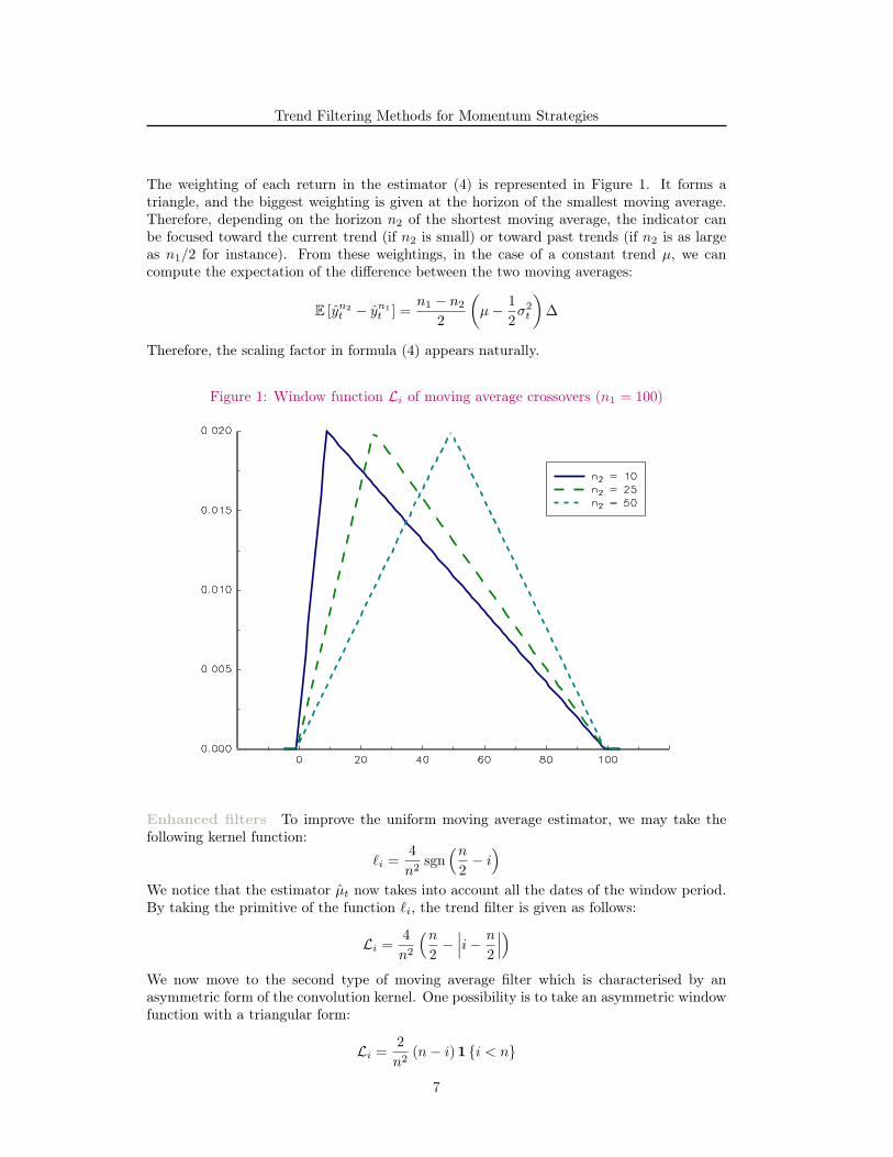
The weighting of each return in the estimator (4) is represented in Figure 1. It forms atriangle, and the biggest weighting is given at the horizon of the smallest moving average.Therefore, depending on the horizon n2 of the shortest moving average, the indicator canbe focused toward the current trend (if n2 is small) or toward past trends (if n2 is as largeas n1/2 for instance). From these weightings, in the case of a constant trend µ, we cancompute the expectation of the difference between the two moving averages:

E [yn2t − yn1

t ] =n1 − n2

2

(µ− 1

2σ2t

)∆

Therefore, the scaling factor in formula (4) appears naturally.

Figure 1: Window function Li of moving average crossovers (n1 = 100)

Enhanced filters To improve the uniform moving average estimator, we may take thefollowing kernel function:

ℓi =4

n2sgn

(n2− i)

We notice that the estimator µt now takes into account all the dates of the window period.By taking the primitive of the function ℓi, the trend filter is given as follows:

Li =4

n2

(n2−∣∣∣i− n

2

∣∣∣)We now move to the second type of moving average filter which is characterised by anasymmetric form of the convolution kernel. One possibility is to take an asymmetric windowfunction with a triangular form:

Li =2

n2(n− i)1 i < n

7


By computing the derivative of this window function, we obtain the following kernel:

ℓi =2

n(δi − 1 i < n)

The filtering equation of µt then becomes:

µt =2

n

(xt −

1

n

n−1∑i=0

xt−i

)

Remark 4 Another way to define µt is to consider the Lanczos generalised derivative(Groetsch, 1998). Let f (x) be a function. We define the Lanczos derivative of f (x) interms of the following relationship:

dL

dxf (x) = lim

ε→0

3

2ε3

∫ ε

−ε

tf (x+ t) dt

In the discrete case, we have:

dL

dxf (x) = lim

h→0

∑nk=−n kf (x+ kh)

2∑n

k=1 k2h

We first notice that the Lanczos derivative is more general than the traditional derivative.Although Lanczos’ formula is a more onerous method for finding the derivative, it offerssome advantages. This technique allows us to compute a “pseudo-derivative” at points wherethe function is not differentiable. For the observable signal yt, the traditional derivative doesnot exist because of the noise εt, but does in the case of the Lanczos derivative. Let us applythe Lanczos’ formula to estimate the derivative of the trend at the point t−T/2. We obtain:

dL

dtxt =

12

n3

n∑i=0

(n2− i)yt−i

We deduce that the kernel is:

ℓi =12

n3

(n2− i)1 0 ≤ i ≤ n

By computing an integration by parts, we obtain the trend filter:

Li =6

n3i (n− i)1 0 ≤ i ≤ n

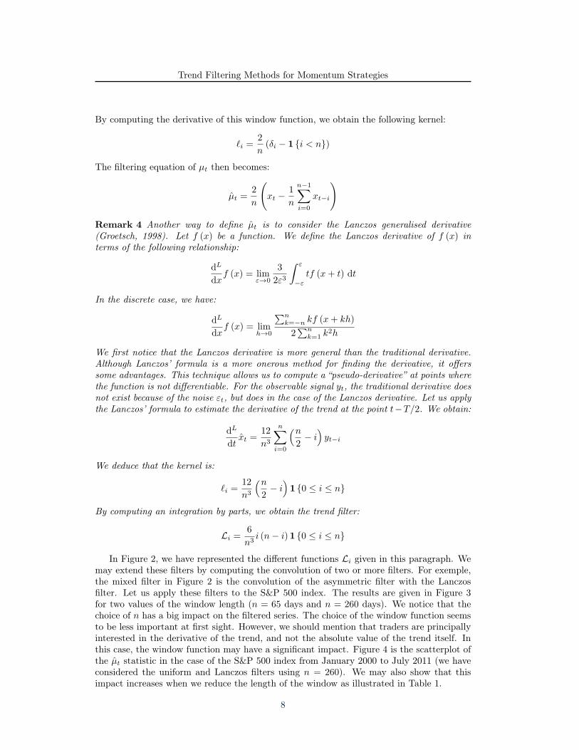
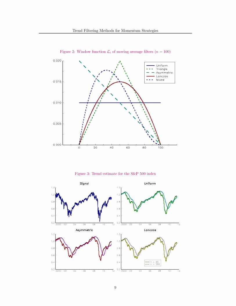
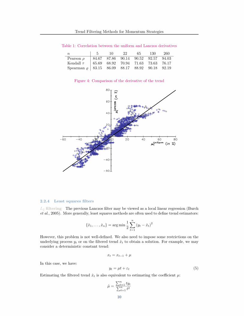
In Figure 2, we have represented the different functions Li given in this paragraph. Wemay extend these filters by computing the convolution of two or more filters. For exemple,the mixed filter in Figure 2 is the convolution of the asymmetric filter with the Lanczosfilter. Let us apply these filters to the S&P 500 index. The results are given in Figure 3for two values of the window length (n = 65 days and n = 260 days). We notice that thechoice of n has a big impact on the filtered series. The choice of the window function seemsto be less important at first sight. However, we should mention that traders are principallyinterested in the derivative of the trend, and not the absolute value of the trend itself. Inthis case, the window function may have a significant impact. Figure 4 is the scatterplot ofthe µt statistic in the case of the S&P 500 index from January 2000 to July 2011 (we haveconsidered the uniform and Lanczos filters using n = 260). We may also show that thisimpact increases when we reduce the length of the window as illustrated in Table 1.

8


Figure 2: Window function Li of moving average filters (n = 100)

Figure 3: Trend estimate for the S&P 500 index

9


Table 1: Correlation between the uniform and Lanczos derivatives

n 5 10 22 65 130 260Pearson ρ 84.67 87.86 90.14 90.52 92.57 94.03Kendall τ 65.69 68.92 70.94 71.63 73.63 76.17Spearman ϱ 83.15 86.09 88.17 88.92 90.18 92.19

Figure 4: Comparison of the derivative of the trend

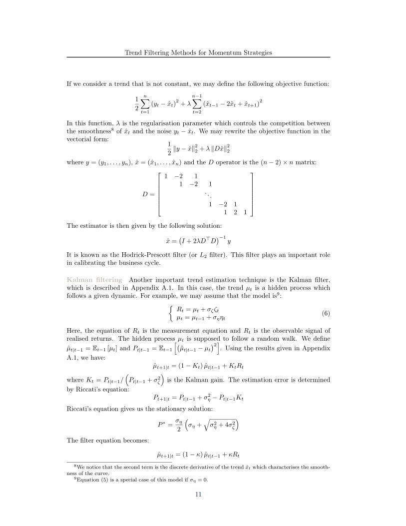
2.2.4 Least squares filters

L2 filtering The previous Lanczos filter may be viewed as a local linear regression (Burchet al., 2005). More generally, least squares methods are often used to define trend estimators:

x1, . . . , xn = argmin1

2

n∑t=1

(yt − xt)2

However, this problem is not well-defined. We also need to impose some restrictions on theunderlying process yt or on the filtered trend xt to obtain a solution. For example, we mayconsider a deterministic constant trend:

xt = xt−1 + µ

In this case, we have:yt = µt+ εt (5)

Estimating the filtered trend xt is also equivalent to estimating the coefficient µ:

µ =

∑nt=1 tyt∑nt=1 t

2

10


If we consider a trend that is not constant, we may define the following objective function:

1

2

n∑t=1

(yt − xt)2+ λ

n−1∑t=2

(xt−1 − 2xt + xt+1)2

In this function, λ is the regularisation parameter which controls the competition betweenthe smoothness8 of xt and the noise yt − xt. We may rewrite the objective function in thevectorial form:

1

2∥y − x∥22 + λ ∥Dx∥22

where y = (y1, . . . , yn), x = (x1, . . . , xn) and the D operator is the (n− 2)× n matrix:

D =

1 −2 1

1 −2 1. . .1 −2 1

1 2 1

The estimator is then given by the following solution:

x =(I + 2λD⊤D

)−1y

It is known as the Hodrick-Prescott filter (or L2 filter). This filter plays an important rolein calibrating the business cycle.

Kalman filtering Another important trend estimation technique is the Kalman filter,which is described in Appendix A.1. In this case, the trend µt is a hidden process whichfollows a given dynamic. For example, we may assume that the model is9:

Rt = µt + σζζtµt = µt−1 + σηηt

(6)

Here, the equation of Rt is the measurement equation and Rt is the observable signal ofrealised returns. The hidden process µt is supposed to follow a random walk. We defineµt|t−1 = Et−1 [µt] and Pt|t−1 = Et−1

[(µt|t−1 − µt

)2]. Using the results given in AppendixA.1, we have:

µt+1|t = (1−Kt) µt|t−1 +KtRt

where Kt = Pt|t−1/(Pt|t−1 + σ2

ζ

)is the Kalman gain. The estimation error is determined

by Riccati’s equation:Pt+1|t = Pt|t−1 + σ2

η − Pt|t−1Kt

Riccati’s equation gives us the stationary solution:

P ∗ =ση2

(ση +

√σ2η + 4σ2

ζ

)The filter equation becomes:

µt+1|t = (1− κ) µt|t−1 + κRt

8We notice that the second term is the discrete derivative of the trend xt which characterises the smooth-ness of the curve.

9Equation (5) is a special case of this model if ση = 0.

11


with:κ =

2ση

ση +√σ2η + 4σ2

ζ

This Kalman filter can be considered as an exponential moving average filter with parame-ter10 λ = − ln (1− κ):

µt =(1− e−λ

) ∞∑i=0

e−λiRt−i

with11 µt = Et [µt]. The filter of the trend xt is therefore determined by the followingequation:

xt =(1− e−λ

) ∞∑i=0

e−λiyt−i

while the derivative of the trend may be directly related to the observed signal yt as follows:

µt =(1− e−λ

)yt −

(1− e−λ

) (eλ − 1

) ∞∑i=1

e−λiyt−i

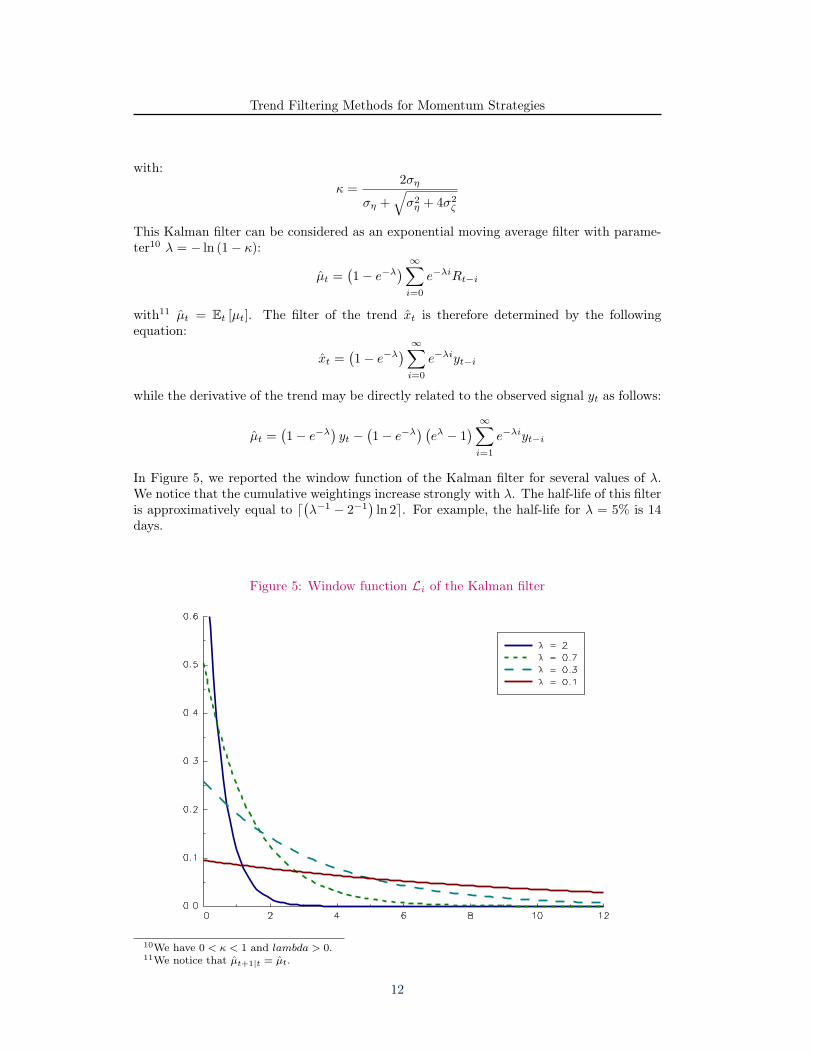
In Figure 5, we reported the window function of the Kalman filter for several values of λ.We notice that the cumulative weightings increase strongly with λ. The half-life of this filteris approximatively equal to ⌈

(λ−1 − 2−1

)ln 2⌉. For example, the half-life for λ = 5% is 14

days.

Figure 5: Window function Li of the Kalman filter

10We have 0 < κ < 1 and lambda > 0.11We notice that µt+1|t = µt.

12


We may wonder what the link is between the regression model (5) and the Markov model(6). Equation (5) is equivalent to the following state space model12:

yt = xt + σεεtxt = xt−1 + µ

If we now consider that the trend is stochastic, the model becomes:yt = xt + σεεtxt = xt−1 + µ+ σζζt

This model is called the local level model. We may also assume that the slope of the trendis stochastic, in which case we obtain the local linear trend model: yt = xt + σεεt

xt = xt−1 + µt−1 + σζζtµt = µt−1 + σηηt

These three models are special cases of structural models (Harvey, 1989) and may be easilysolved by Kalman filtering. We also deduce that the Markov model (6) is a special case ofthe latter when σε = 0.

Remark 5 We have shown that Kalman filtering may be viewed as an exponential movingaverage filter when we consider the Markov model (6). Nevertheless, we cannot regard theKalman filter simply as a moving average filter. First, the Kalman filter is the optimalfilter in the case of the linear Gaussian model described in Appendix A.1. Second, it couldbe regarded as “an efficient computational solution of the least squares method” (Sorensen,1970). Third, we could use it to solve more sophisticated processes than the Markov model(6). However, some nonlinear or non Gaussian models may be too complex for Kalmanfiltering. These nonlinear models can be solved by particle filters or sequential Monte Carlomethods (see Doucet et al., 1998).

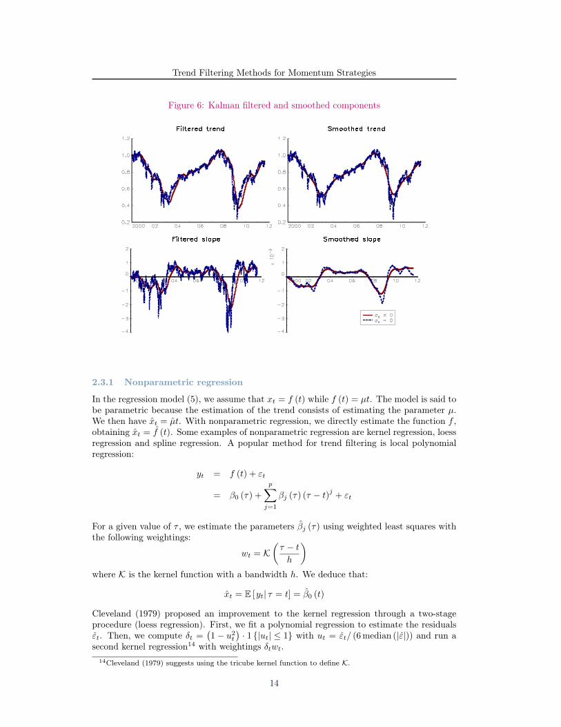
Another important feature of the Kalman approach is the derivation of an optimalsmoother (see Appendix A.1). At time t, we are interested by the numerical value of xt, butalso by the past values of xt−i because we would like to measure the slope of the trend. TheKalman smoother improves the estimate of xt−i by using all the information between t− iand t. Let us consider the previous example in relation to the S&P 500 index, using the locallevel model. Figure 6 gives the filtered and smoothed components xt and µt for two setsof parameters13. We verify that the Kalman smoother reduces the noise by incorporatingmore information. We also notice that the restriction σε = 0 increases the variance of thetrend and slope estimators.

2.3 Nonlinear filtering

In this section, we review other filtering approaches. They are generally classed as nonlinearfilters, because it is not possible to express the trend as a linear convolution of the signaland a window function.

12In what follows, the noise processes are white noise: εt ∼ N (0, 1), ζt ∼ N (0, 1) and ηt ∼ N (0, 1).13For the first set of parameters, we assume that σε = 100σζ and ση = 1/100σζ . For the second set of

parameters, we impose the restriction σε = 0.

13


Figure 6: Kalman filtered and smoothed components

2.3.1 Nonparametric regression

In the regression model (5), we assume that xt = f (t) while f (t) = µt. The model is said tobe parametric because the estimation of the trend consists of estimating the parameter µ.We then have xt = µt. With nonparametric regression, we directly estimate the function f ,obtaining xt = f (t). Some examples of nonparametric regression are kernel regression, loessregression and spline regression. A popular method for trend filtering is local polynomialregression:

yt = f (t) + εt

= β0 (τ) +

p∑j=1

βj (τ) (τ − t)j+ εt

For a given value of τ , we estimate the parameters βj (τ) using weighted least squares withthe following weightings:

wt = K(τ − t

h

)where K is the kernel function with a bandwidth h. We deduce that:

xt = E [yt| τ = t] = β0 (t)

Cleveland (1979) proposed an improvement to the kernel regression through a two-stageprocedure (loess regression). First, we fit a polynomial regression to estimate the residualsεt. Then, we compute δt =

(1− u2t

)· 1 |ut| ≤ 1 with ut = εt/ (6median (|ε|)) and run a

second kernel regression14 with weightings δtwt.14Cleveland (1979) suggests using the tricube kernel function to define K.

14


A spline function is a C2 function S (τ) which corresponds to a cubic polynomial functionon each interval [t, t+ 1[. Let SP be the set of spline functions. We then have to solve thefollowing optimisation programme:

minS∈SP

(1− h)n∑

t=0

wt (yt − S (t))2+ h

∫ T

0

wτS′′ (τ)

2dτ

where h is the smoothing parameter – h = 0 corresponds to the interpolation case15 andh = 1 corresponds to the linear regression16.

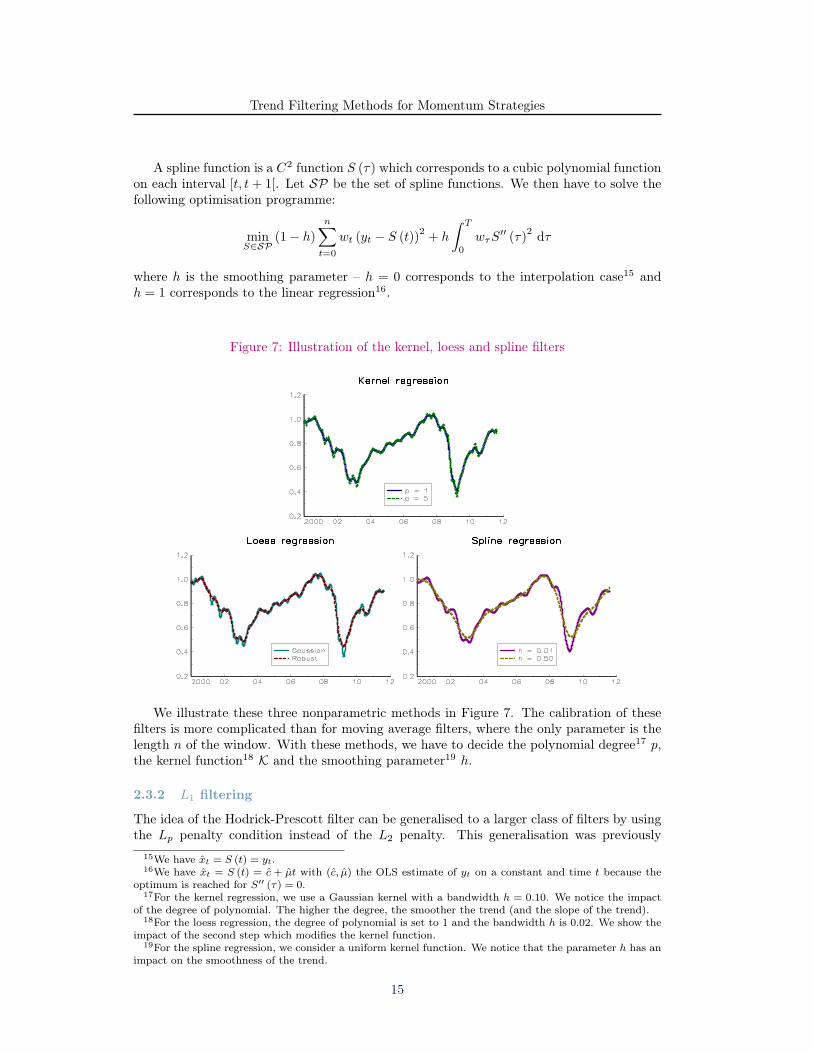
Figure 7: Illustration of the kernel, loess and spline filters

We illustrate these three nonparametric methods in Figure 7. The calibration of thesefilters is more complicated than for moving average filters, where the only parameter is thelength n of the window. With these methods, we have to decide the polynomial degree17 p,the kernel function18 K and the smoothing parameter19 h.

2.3.2 L1 filtering

The idea of the Hodrick-Prescott filter can be generalised to a larger class of filters by usingthe Lp penalty condition instead of the L2 penalty. This generalisation was previously

15We have xt = S (t) = yt.16We have xt = S (t) = c + µt with (c, µ) the OLS estimate of yt on a constant and time t because the

optimum is reached for S′′ (τ) = 0.17For the kernel regression, we use a Gaussian kernel with a bandwidth h = 0.10. We notice the impact

of the degree of polynomial. The higher the degree, the smoother the trend (and the slope of the trend).18For the loess regression, the degree of polynomial is set to 1 and the bandwidth h is 0.02. We show the

impact of the second step which modifies the kernel function.19For the spline regression, we consider a uniform kernel function. We notice that the parameter h has an

impact on the smoothness of the trend.

15


discussed in the work of Daubechies et al. (2004) in relation to the linear inverse problem,while Tibshirani (1996) considers the Lasso regression problem. If we consider an L1 filter,the objective function becomes:

1

2

n∑t=1

(yt − xt)2+ λ

n−1∑t=2

|xt−1 − 2xt + xt+1|

which is equivalent to the following vectorial form:

1

2∥y − x∥22 + λ ∥Dx∥1

Kim et al. (2009) shows that the dual problem of this L1 filter scheme is a quadraticprogramme with some boundary constraints20. To find x, we may also use the quadraticprogramming algorithm, but Kim et al. (2009) suggest using the primal-dual interior pointmethod in order to optimise the numerical computation speed.

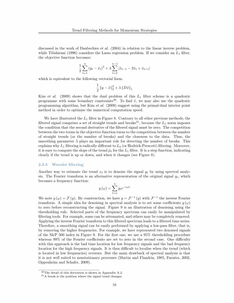
We have illustrated the L1 filter in Figure 8. Contrary to all other previous methods, thefiltered signal comprises a set of straight trends and breaks21, because the L1 norm imposesthe condition that the second derivative of the filtered signal must be zero. The competitionbetween the two terms in the objective function turns to the competition between the numberof straight trends (or the number of breaks) and the closeness to the data. Thus, thesmoothing parameter λ plays an important role for detecting the number of breaks. Thisexplains why L1 filtering is radically different to L2 (or Hodrick-Prescott) filtering. Moreover,it is easy to compute the slope of the trend µt for the L1 filter. It is a step function, indicatingclearly if the trend is up or down, and when it changes (see Figure 8).

2.3.3 Wavelet filtering

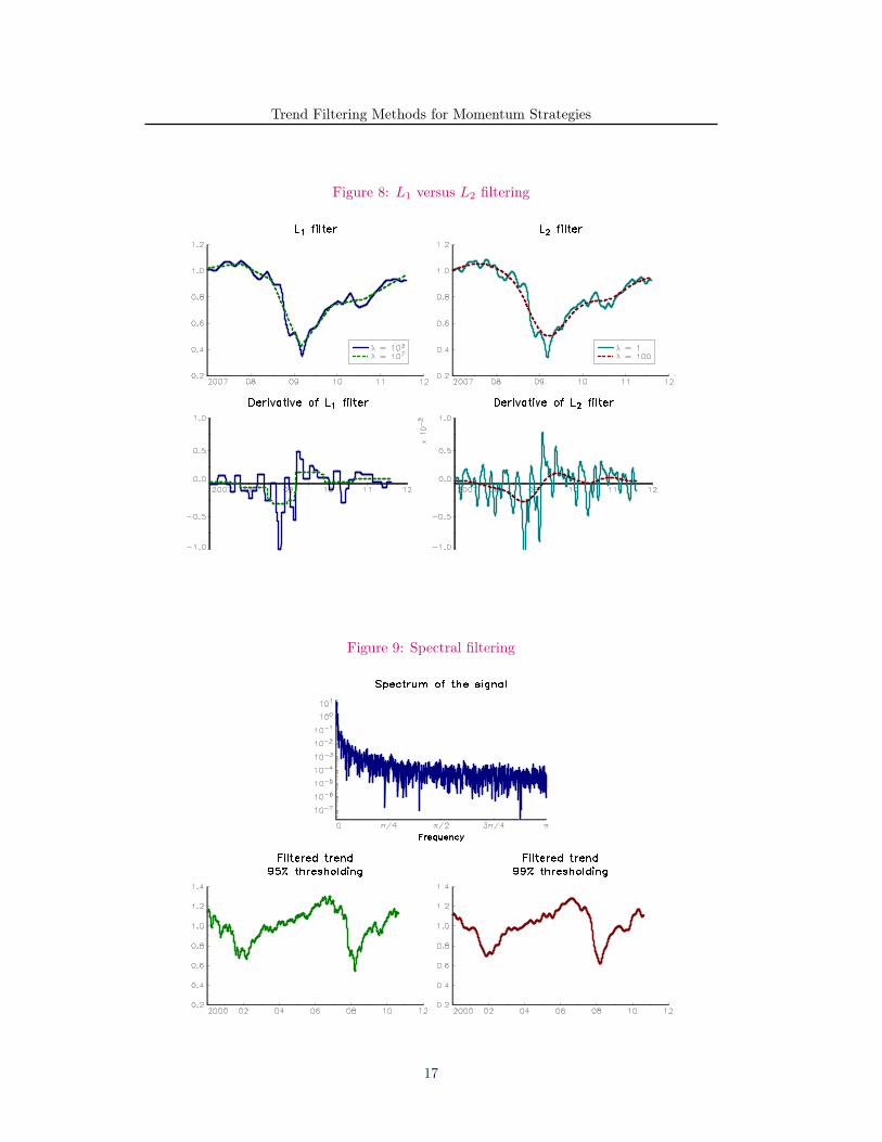
Another way to estimate the trend xt is to denoise the signal yt by using spectral analy-sis. The Fourier transform is an alternative representation of the original signal yt, whichbecomes a frequency function:

y (ω) =n∑

t=1

yte−iωt

We note y (ω) = F (y). By construction, we have y = F−1 (y) with F−1 the inverse Fouriertransform. A simple idea for denoising in spectral analysis is to set some coefficients y (ω)to zero before reconstructing the signal. Figure 9 is an illustration of denoising using thethresholding rule. Selected parts of the frequency spectrum can easily be manipulated byfiltering tools. For example, some can be attenuated, and others may be completely removed.Applying the inverse Fourier transform to this filtered spectrum leads to a filtered time series.Therefore, a smoothing signal can be easily performed by applying a low-pass filter, that is,by removing the higher frequencies. For example, we have represented two denoised signalsof the S&P 500 index in Figure 9. For the first one, we use a 95% thresholding procedurewhereas 99% of the Fourier coefficients are set to zero in the second case. One difficultywith this approach is the bad time location for low frequency signals and the bad frequencylocation for the high frequency signals. It is then difficult to localise when the trend (whichis located in low frequencies) reverses. But the main drawback of spectral analysis is thatit is not well suited to nonstationary processes (Martin and Flandrin, 1985, Fuentes, 2002,Oppenheim and Schafer, 2009).

20The detail of this derivation is shown in Appendix A.2.21A break is the position where the signal trend changes.

16


Figure 8: L1 versus L2 filtering

Figure 9: Spectral filtering

17


A solution consists of adopting a double dimension analysis, both in time and frequency.This approach corresponds to the wavelet analysis. The method of denoising is the same asdescribed previously and the estimation of xt is done in three steps:

1. we compute the wavelet transform W of the original signal yt to obtain the waveletcoefficients ω = W (y);

2. we modify the wavelet coefficients according to a denoising rule D:

ω⋆ = D (ω)

3. We convert the modified wavelet coefficients into a new signal using the inverse wavelettransform W−1:

x = W−1 (ω⋆)

There are two principal choices in this approach. First, we have to specify which motherwavelet to use. Second, we have to define the denoising rule. Let ω− and ω+ be two scalarswith 0 < ω− < ω+. Donoho and Johnstone (1995) define several shrinkage methods22:

• Hard shrinkageω⋆i = ωi · 1

|ωi| > ω+

• Soft shrinkage

ω⋆i = sgn (ωi) ·

(|ωi| − ω+

)+

• Semi-soft shrinkage

ω⋆i =

0 si |ωi| ≤ ω−

sgn (ωi) (ω+ − ω−)

−1ω+ (|ωi| − ω−) si ω− < |ωi| ≤ ω+

ωi si |ωi| > ω+

• Quantile shrinkage is a hard shrinkage method where w+ is the qth quantile of thecoefficients |ωi|.

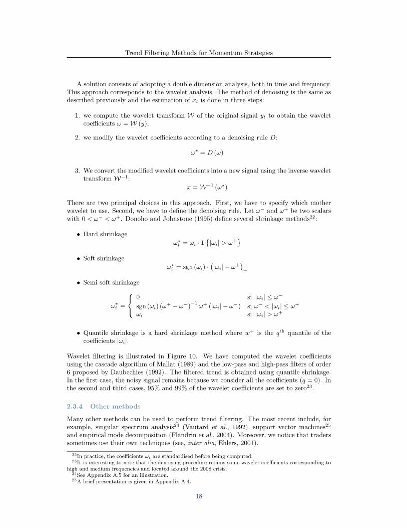
Wavelet filtering is illustrated in Figure 10. We have computed the wavelet coefficientsusing the cascade algorithm of Mallat (1989) and the low-pass and high-pass filters of order6 proposed by Daubechies (1992). The filtered trend is obtained using quantile shrinkage.In the first case, the noisy signal remains because we consider all the coefficients (q = 0). Inthe second and third cases, 95% and 99% of the wavelet coefficients are set to zero23.

2.3.4 Other methods

Many other methods can be used to perform trend filtering. The most recent include, forexample, singular spectrum analysis24 (Vautard et al., 1992), support vector machines25and empirical mode decomposition (Flandrin et al., 2004). Moreover, we notice that traderssometimes use their own techniques (see, inter alia, Ehlers, 2001).

22In practice, the coefficients ωi are standardised before being computed.23It is interesting to note that the denoising procedure retains some wavelet coefficients corresponding to

high and medium frequencies and located around the 2008 crisis.24See Appendix A.5 for an illustration.25A brief presentation is given in Appendix A.4.

18


Figure 10: Wavelet filtering

2.4 Multivariate filtering

Until now, we have assumed that the trend is specific to a financial asset. However, we maybe interested in estimating the common trend of several financial assets. For example, if wewanted to estimate the trend of emerging markets equities, we could use a global index likethe MSCI EM or extract the trend by considering several indices, e.g. the Bovespa index(Brazil), the RTS index (Russia), the Nifty index (India), the HSCEI index (China), etc. Inthis case, the trend-cycle model becomes:

y(1)t...

y(m)t

= xt +

ε(1)t...

ε(m)t

where y(j)t and ε(j)t are respectively the signal and the noise of the financial asset j and xt

is the common trend. One idea for estimating the common trend is to obtain the mean ofthe specific trends:

xt =1

m

m∑j=1

x(j)t

19


If we consider moving average filtering, it is equivalent to applying the filter to the averagefilter26 yt = 1

m

∑mj=1 y

(j)t . This rule is also valid for some nonlinear filters such as L1 filtering

(see Appendix A.2). In what follows, we consider the two main alternative approachesdeveloped in econometrics to estimate a (stochastic) common trend.

2.4.1 Error-correction model, common factors and the P-T decomposition

The econometrics of nonstationary time series may also help us to estimate a common trend.y(j)t is said to be integrated of order 1 if the change y(j)t − y

(j)t−1 is stationary. We will note

y(j)t ∼ I (1) and (1− L) y

(j)t ∼ I (0). Let us now define yt =

(y(1)t , . . . , y

(m)t

). The vector yt

is cointegrated of rank r if there exists a matrix β of rank r such that zt = β⊤yt ∼ I (0).In this case, we show that yt may be specified by an error-correction model (Engle andGranger, 1987):

∆yt = γzt−1 +∞∑i=1

Φi∆yt−i + ζt (7)

where ζt is a I (0) vector process. Stock and Watson (1988) propose another interestingrepresentation of cointegration systems. Let ft be a vector of r common factors which areI (1). Therefore, we have:

yt = Aft + ηt (8)

where ηt is a I (0) vector process and ft is a I (1) vector process. One of the difficulties withthis type of model is the identification step (Peña and Box, 1987). Gonzalo and Granger(1995) suggest defining a permanent-transitory (P-T) decomposition:

yt = Pt + Tt

such that the permanent component Pt is difference stationary, the transitory component Ttis covariance stationary and (∆Pt, Tt) satisfies a constrained autoregressive representation.Using this framework and some other conditions, Gonzalo and Granger show that we mayobtain the representation (8) by estimating the relationship (7):

ft = γ⊤yt (9)

where γ⊤γ = 0. They then follow the works of Johansen (1988, 1991) to derive the maximumlikelihood estimator of γ. Once we have estimated the relationship (9), it is also easy toidentify the common trend27 xt.

26We have:

xt =1

m

m∑j=1

n−1∑i=0

Liy(j)t−i

=

n−1∑i=0

Li

1

m

m∑j=1

y(j)t−i

=

n−1∑i=0

Liyt−i

27If a common trend exists, it is necessarily one of the common factors.

20


2.4.2 Common stochastic trend model

Another idea is to consider an extension of the local linear trend model: yt = αxt + εtxt = xt−1 + µt−1 + σζζtµt = µt−1 + σηηt

with yt =(y(1)t , . . . , y

(m)t

), εt =

(ε(1)t , . . . , ε

(m)t

)∼ N (0,Ω), ζt ∼ N (0, 1) and ηt ∼ N (0, 1).

Moreover, we assume that εt, ζt and ηt are independent of each other. Given the parameters(α,Ω, σζ , ση), we may run the Kalman filter to estimate the trend xt and the slope µt whereasthe Kalman smoother allows us to estimate xt−i and µt−i at time t.

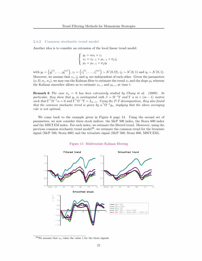
Remark 6 The case ση = 0 has been extensively studied by Chang et al. (2009). Inparticular, they show that yt is cointegrated with β = Ω−1Γ and Γ a m × (m− 1) matrixsuch that Γ⊤Ω−1α = 0 and Γ⊤Ω−1Γ = Im−1. Using the P-T decomposition, they also foundthat the common stochastic trend is given by α⊤Ω−1yt, implying that the above averagingrule is not optimal.

We come back to the example given in Figure 6 page 14. Using the second set ofparameters, we now consider three stock indices: the S&P 500 index, the Stoxx 600 indexand the MSCI EM index. For each index, we estimate the filtered trend. Moreover, using theprevious common stochastic trend model28, we estimate the common trend for the bivariatesignal (S&P 500, Stoxx 600) and the trivariate signal (S&P 500, Stoxx 600, MSCI EM).

Figure 11: Multivariate Kalman filtering

28We assume that αj takes the value 1 for the three signals.

21


3 Trend filtering in practice

3.1 The calibration problem

For the practical use of the trend extraction techniques discussed above, the calibration offiltering parameters is crucial. These calibrated parameters must incorporate our predictionrequirement or they can be mapped to a commonly-known benchmark estimator. Theseconstraints offer us some criteria for determining the optimal parameters for our expectedprediction horizon. Below, we consider two possible calibration schemes based on thesecriteria.

3.1.1 Calibration based on prediction error

One idea for estimating the parameters of a model is to use statistical inference tools. Letus consider the local linear trend model. We may estimate the set of parameters (σε, σζ , ση)by maximising the log-likelihood function29:

ℓ =1

2

n∑t=1

ln 2π + lnFt +v2tFt

where vt = yt − Et−1 [yt] is the innovation process and Ft = Et−1

[v2t]

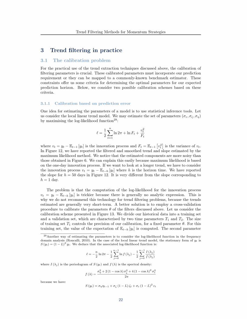
is the variance of vt.In Figure 12, we have reported the filtered and smoothed trend and slope estimated by themaximum likelihood method. We notice that the estimated components are more noisy thanthose obtained in Figure 6. We can explain this easily because maximum likelihood is basedon the one-day innovation process. If we want to look at a longer trend, we have to considerthe innovation process vt = yt − Et−h [yt] where h is the horizon time. We have reportedthe slope for h = 50 days in Figure 12. It is very different from the slope corresponding toh = 1 day.

The problem is that the computation of the log-likelihood for the innovation processvt = yt − Et−h [yt] is trickier because there is generally no analytic expression. This iswhy we do not recommend this technology for trend filtering problems, because the trendsestimated are generally very short-term. A better solution is to employ a cross-validationprocedure to calibrate the parameters θ of the filters discussed above. Let us consider thecalibration scheme presented in Figure 13. We divide our historical data into a training setand a validation set, which are characterised by two time parameters T1 and T2. The sizeof training set T1 controls the precision of our calibration, for a fixed parameter θ. For thistraining set, the value of the expectation of Et−h [yt] is computed. The second parameter

29Another way of estimating the parameters is to consider the log-likelihood function in the frequencydomain analysis (Roncalli, 2010). In the case of the local linear trend model, the stationary form of yt isS (yt) = (1− L)2 yt. We deduce that the associated log-likelihood function is:

ℓ = −n

2ln 2π −

1

2

n−1∑j=0

ln f (λj)−1

2

n−1∑j=0

I (λj)

f (λj)

where I (λj) is the periodogram of S (yt) and f (λ) is the spectral density:

f (λ) =σ2η + 2 (1− cosλ)σ2

ζ + 4 (1− cosλ)2 σ2ε

2π

because we have:S (yt) = σηηt−1 + σζ (1− L) ζt + σε (1− L)2 εt

22


Figure 12: Maximum likelihood of the trend and slope components

T2 determines the size of the validation set, which is used to estimate the prediction error:

e (θ;h) =n−h∑t=1

(yt − Et−h [yt])2

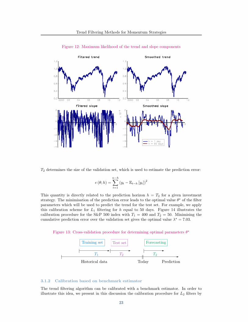
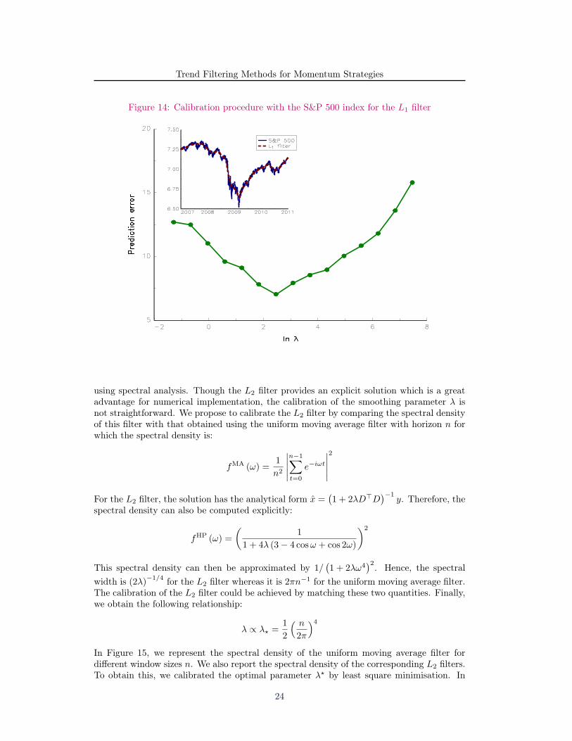
This quantity is directly related to the prediction horizon h = T2 for a given investmentstrategy. The minimisation of the prediction error leads to the optimal value θ⋆ of the filterparameters which will be used to predict the trend for the test set. For example, we applythis calibration scheme for L1 filtering for h equal to 50 days. Figure 14 illustrates thecalibration procedure for the S&P 500 index with T1 = 400 and T2 = 50. Minimising thecumulative prediction error over the validation set gives the optimal value λ⋆ = 7.03.

Figure 13: Cross-validation procedure for determining optimal parameters θ⋆

| -∥| -

T1

Training set

| -T2

Test set

| -T2

Forecasting

Historical data Today Prediction

3.1.2 Calibration based on benchmark estimator

The trend filtering algorithm can be calibrated with a benchmark estimator. In order toillustrate this idea, we present in this discussion the calibration procedure for L2 filters by

23


Figure 14: Calibration procedure with the S&P 500 index for the L1 filter

using spectral analysis. Though the L2 filter provides an explicit solution which is a greatadvantage for numerical implementation, the calibration of the smoothing parameter λ isnot straightforward. We propose to calibrate the L2 filter by comparing the spectral densityof this filter with that obtained using the uniform moving average filter with horizon n forwhich the spectral density is:

fMA (ω) =1

n2

∣∣∣∣∣n−1∑t=0

e−iωt

∣∣∣∣∣2

For the L2 filter, the solution has the analytical form x =(1 + 2λD⊤D

)−1y. Therefore, the

spectral density can also be computed explicitly:

fHP (ω) =

(1

1 + 4λ (3− 4 cosω + cos 2ω)

)2

This spectral density can then be approximated by 1/(1 + 2λω4

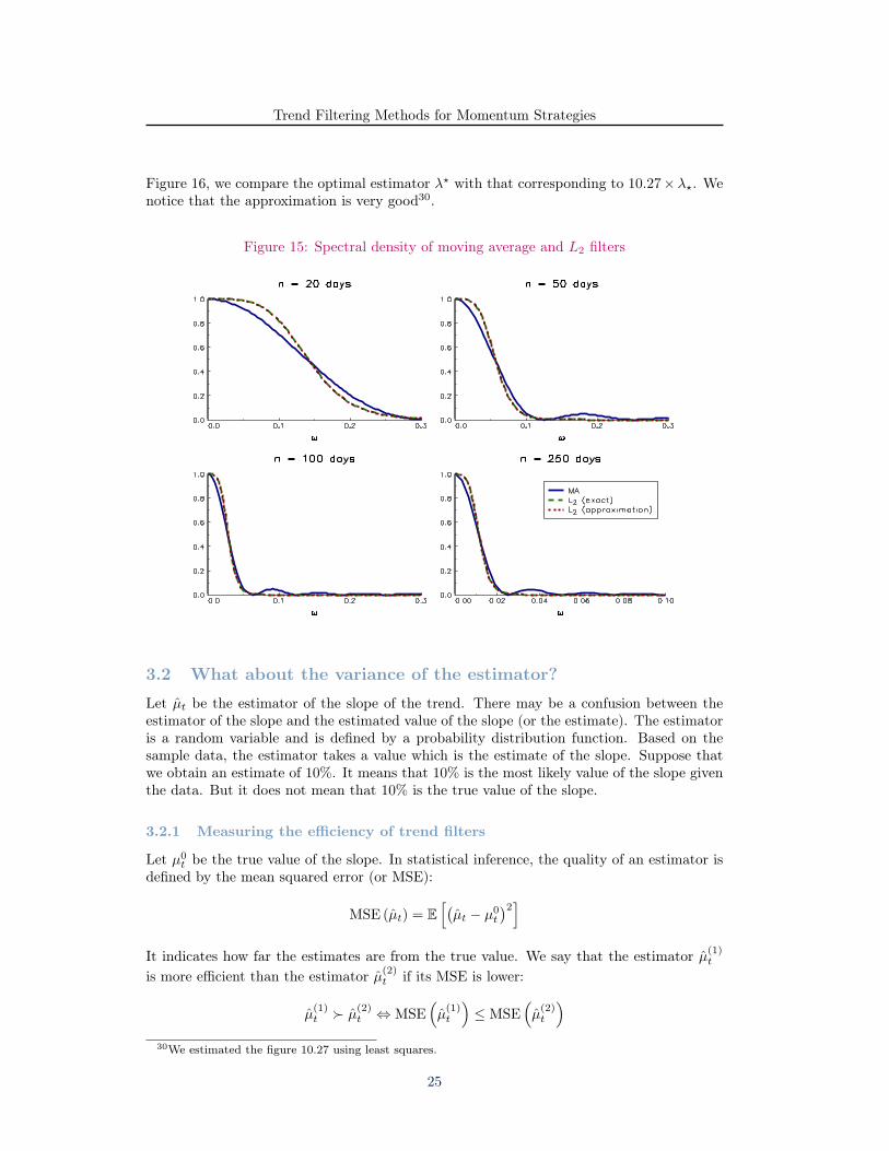
)2. Hence, the spectralwidth is (2λ)−1/4 for the L2 filter whereas it is 2πn−1 for the uniform moving average filter.The calibration of the L2 filter could be achieved by matching these two quantities. Finally,we obtain the following relationship:

λ ∝ λ⋆ =1

2

( n2π

)4In Figure 15, we represent the spectral density of the uniform moving average filter fordifferent window sizes n. We also report the spectral density of the corresponding L2 filters.To obtain this, we calibrated the optimal parameter λ⋆ by least square minimisation. In

24


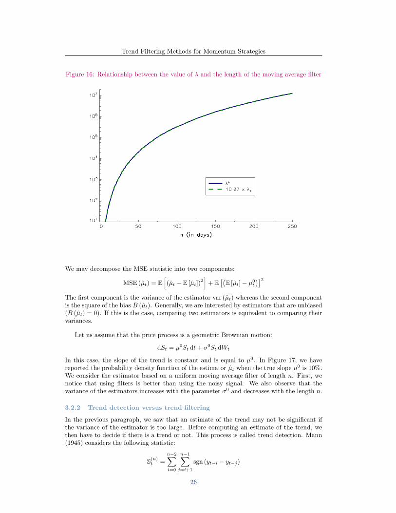
Figure 16, we compare the optimal estimator λ⋆ with that corresponding to 10.27× λ⋆. Wenotice that the approximation is very good30.

Figure 15: Spectral density of moving average and L2 filters

3.2 What about the variance of the estimator?

Let µt be the estimator of the slope of the trend. There may be a confusion between theestimator of the slope and the estimated value of the slope (or the estimate). The estimatoris a random variable and is defined by a probability distribution function. Based on thesample data, the estimator takes a value which is the estimate of the slope. Suppose thatwe obtain an estimate of 10%. It means that 10% is the most likely value of the slope giventhe data. But it does not mean that 10% is the true value of the slope.

3.2.1 Measuring the efficiency of trend filters

Let µ0t be the true value of the slope. In statistical inference, the quality of an estimator is

defined by the mean squared error (or MSE):

MSE (µt) = E[(µt − µ0

t

)2]It indicates how far the estimates are from the true value. We say that the estimator µ(1)

t

is more efficient than the estimator µ(2)t if its MSE is lower:

µ(1)t ≻ µ

(2)t ⇔ MSE

(µ(1)t

)≤ MSE

(µ(2)t

)30We estimated the figure 10.27 using least squares.

25


Figure 16: Relationship between the value of λ and the length of the moving average filter

We may decompose the MSE statistic into two components:

MSE (µt) = E[(µt − E [µt])

2]+ E

[(E [µt]− µ0

t

)]2The first component is the variance of the estimator var (µt) whereas the second componentis the square of the bias B (µt). Generally, we are interested by estimators that are unbiased(B (µt) = 0). If this is the case, comparing two estimators is equivalent to comparing theirvariances.

Let us assume that the price process is a geometric Brownian motion:

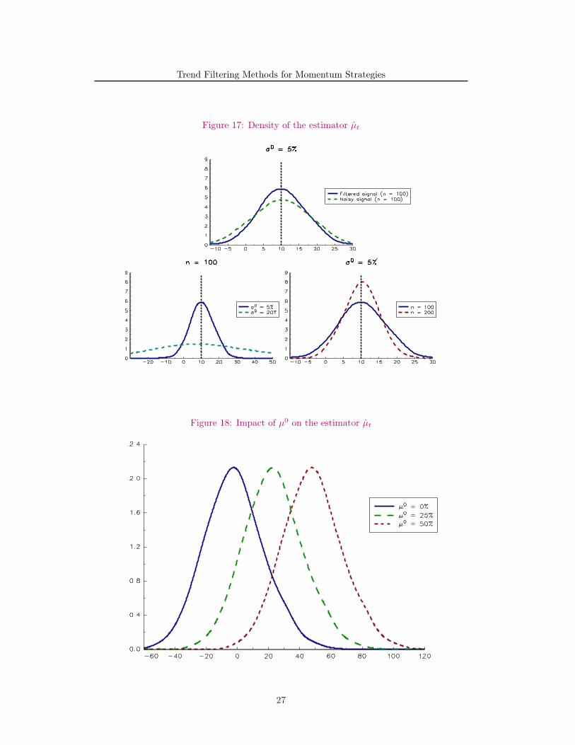
dSt = µ0St dt+ σ0St dWt

In this case, the slope of the trend is constant and is equal to µ0. In Figure 17, we havereported the probability density function of the estimator µt when the true slope µ0 is 10%.We consider the estimator based on a uniform moving average filter of length n. First, wenotice that using filters is better than using the noisy signal. We also observe that thevariance of the estimators increases with the parameter σ0 and decreases with the length n.

3.2.2 Trend detection versus trend filtering

In the previous paragraph, we saw that an estimate of the trend may not be significant ifthe variance of the estimator is too large. Before computing an estimate of the trend, wethen have to decide if there is a trend or not. This process is called trend detection. Mann(1945) considers the following statistic:

S(n)t =n−2∑i=0

n−1∑j=i+1

sgn (yt−i − yt−j)

26


Figure 17: Density of the estimator µt

Figure 18: Impact of µ0 on the estimator µt

27


with sgn (yt−i − yt−j) = 1 if yt−i > yt−j and sgn (yt−i − yt−j) = −1 if yt−i < yt−j . Wehave31:

var(S(n)t

)=n (n− 1) (2n+ 5)

18

We can show that:−n (n+ 1)

2≤ S(n)t ≤ n (n+ 1)

2

The bounds are reached if yt < yt−i (negative trend) or yt > yt−i (positive trend) for i ∈ N∗.We can then normalise the score:

S(n)t =

2S(n)t

n (n+ 1)

S(n)t takes the value +1 (or −1) if we have a perfect positive (or negative) trend. If there is

no trend, it is obvious that S(n)t ≃ 0. Under this null hypothesis, we have:

Z(n)t −→

n→∞N (0, 1)

with:

Z(n)t =

S(n)t√var(S(n)t

)

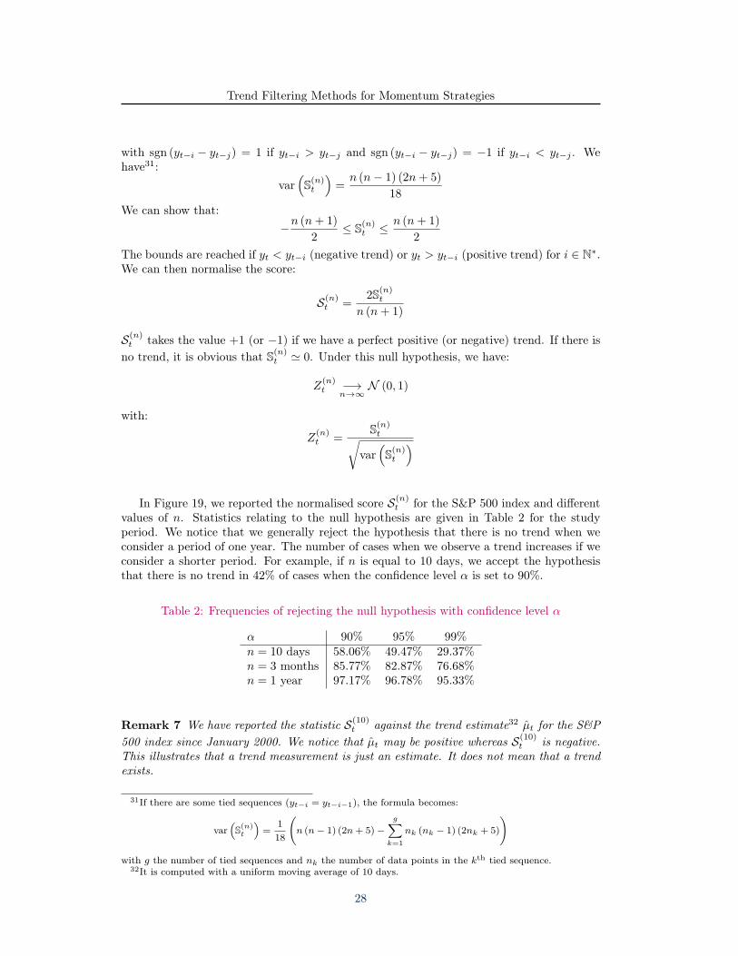
In Figure 19, we reported the normalised score S(n)t for the S&P 500 index and different

values of n. Statistics relating to the null hypothesis are given in Table 2 for the studyperiod. We notice that we generally reject the hypothesis that there is no trend when weconsider a period of one year. The number of cases when we observe a trend increases if weconsider a shorter period. For example, if n is equal to 10 days, we accept the hypothesisthat there is no trend in 42% of cases when the confidence level α is set to 90%.

Table 2: Frequencies of rejecting the null hypothesis with confidence level α

α 90% 95% 99%n = 10 days 58.06% 49.47% 29.37%n = 3 months 85.77% 82.87% 76.68%n = 1 year 97.17% 96.78% 95.33%

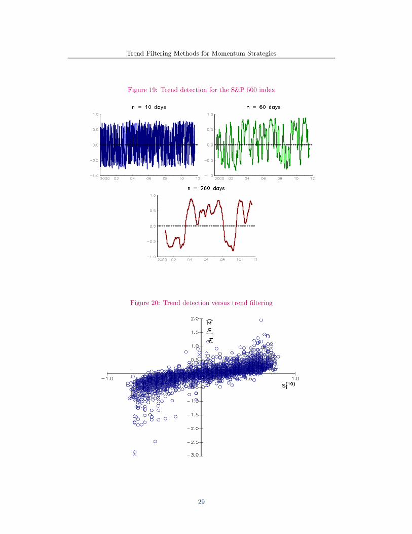
Remark 7 We have reported the statistic S(10)t against the trend estimate32 µt for the S&P

500 index since January 2000. We notice that µt may be positive whereas S(10)t is negative.

This illustrates that a trend measurement is just an estimate. It does not mean that a trendexists.

31If there are some tied sequences (yt−i = yt−i−1), the formula becomes:

var(S(n)t

)=

1

18

(n (n− 1) (2n+ 5)−

g∑k=1

nk (nk − 1) (2nk + 5)

)

with g the number of tied sequences and nk the number of data points in the kth tied sequence.32It is computed with a uniform moving average of 10 days.

28


Figure 19: Trend detection for the S&P 500 index

Figure 20: Trend detection versus trend filtering

29


3.3 From trend filtering to trend forecasting

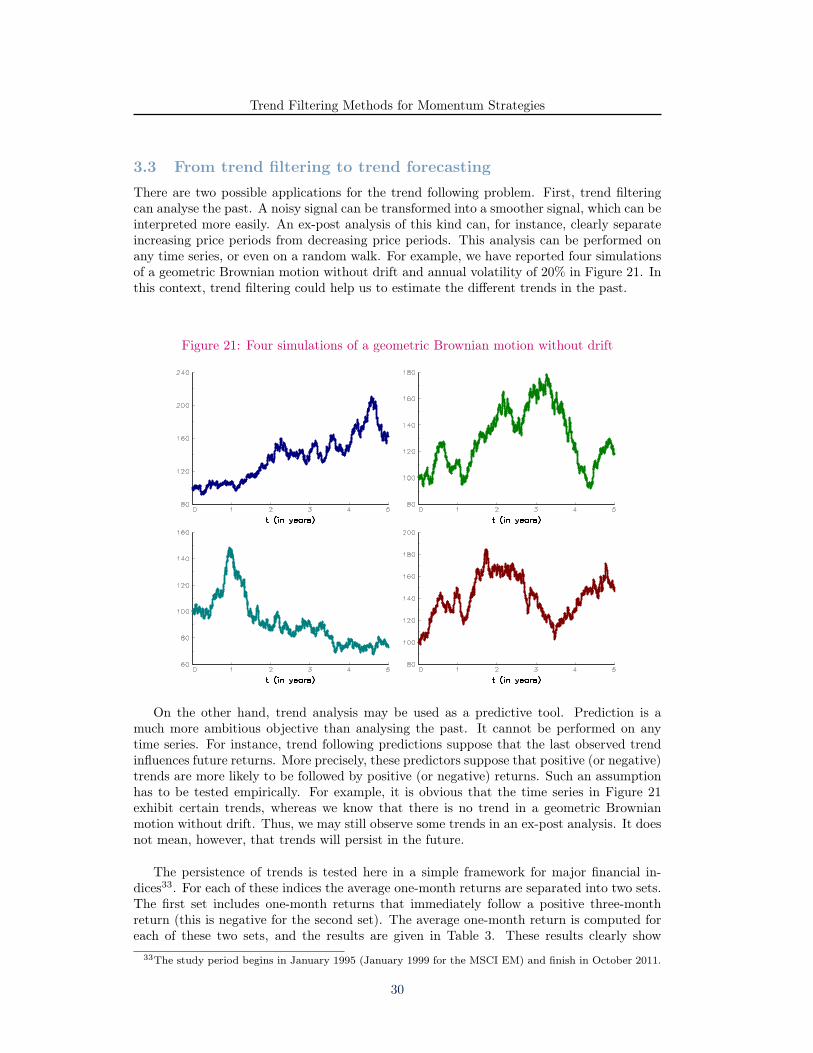
There are two possible applications for the trend following problem. First, trend filteringcan analyse the past. A noisy signal can be transformed into a smoother signal, which can beinterpreted more easily. An ex-post analysis of this kind can, for instance, clearly separateincreasing price periods from decreasing price periods. This analysis can be performed onany time series, or even on a random walk. For example, we have reported four simulationsof a geometric Brownian motion without drift and annual volatility of 20% in Figure 21. Inthis context, trend filtering could help us to estimate the different trends in the past.

Figure 21: Four simulations of a geometric Brownian motion without drift

On the other hand, trend analysis may be used as a predictive tool. Prediction is amuch more ambitious objective than analysing the past. It cannot be performed on anytime series. For instance, trend following predictions suppose that the last observed trendinfluences future returns. More precisely, these predictors suppose that positive (or negative)trends are more likely to be followed by positive (or negative) returns. Such an assumptionhas to be tested empirically. For example, it is obvious that the time series in Figure 21exhibit certain trends, whereas we know that there is no trend in a geometric Brownianmotion without drift. Thus, we may still observe some trends in an ex-post analysis. It doesnot mean, however, that trends will persist in the future.

The persistence of trends is tested here in a simple framework for major financial in-dices33. For each of these indices the average one-month returns are separated into two sets.The first set includes one-month returns that immediately follow a positive three-monthreturn (this is negative for the second set). The average one-month return is computed foreach of these two sets, and the results are given in Table 3. These results clearly show

33The study period begins in January 1995 (January 1999 for the MSCI EM) and finish in October 2011.

30


Figure 22: Distribution of the conditional standardised monthly return

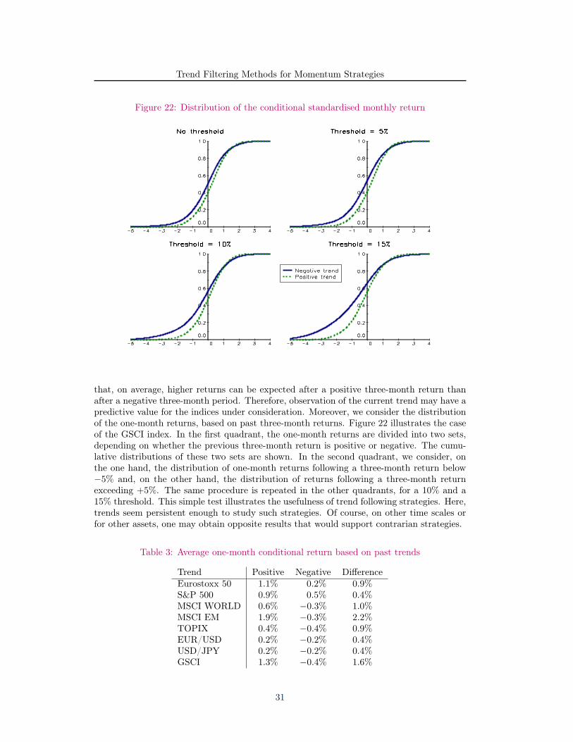
that, on average, higher returns can be expected after a positive three-month return thanafter a negative three-month period. Therefore, observation of the current trend may have apredictive value for the indices under consideration. Moreover, we consider the distributionof the one-month returns, based on past three-month returns. Figure 22 illustrates the caseof the GSCI index. In the first quadrant, the one-month returns are divided into two sets,depending on whether the previous three-month return is positive or negative. The cumu-lative distributions of these two sets are shown. In the second quadrant, we consider, onthe one hand, the distribution of one-month returns following a three-month return below−5% and, on the other hand, the distribution of returns following a three-month returnexceeding +5%. The same procedure is repeated in the other quadrants, for a 10% and a15% threshold. This simple test illustrates the usefulness of trend following strategies. Here,trends seem persistent enough to study such strategies. Of course, on other time scales orfor other assets, one may obtain opposite results that would support contrarian strategies.

Table 3: Average one-month conditional return based on past trends

Trend Positive Negative DifferenceEurostoxx 50 1.1% 0.2% 0.9%S&P 500 0.9% 0.5% 0.4%MSCI WORLD 0.6% −0.3% 1.0%MSCI EM 1.9% −0.3% 2.2%TOPIX 0.4% −0.4% 0.9%EUR/USD 0.2% −0.2% 0.4%USD/JPY 0.2% −0.2% 0.4%GSCI 1.3% −0.4% 1.6%

31


4 ConclusionThe ultimate goal of trend filtering in finance is to design portfolio strategies that maybenefit from these trends. But the path between trend measurement and portfolio allocationis not straightforward. It involves studies and explanations that would not fit in this paper.Nevertheless, let us point out some major issues. Of course, the first problem is the selectionof the trend filtering method. This selection may lead to a single procedure or to a pool ofmethods. The selection of several methods raises the question of an aggregation procedure.This can be done through averaging or dynamic model selection, for instance. The resultingtrend indicator is meant to forecast future asset returns at a given horizon.

Intuitively, an investor should buy assets with positive return forecasts and sell assetswith negative forecasts. But the size of each long or short position is a quantitative problemthat requires a clear investment process. This process should take into account the riskentailed by each position, compared with the expected return. Traditionally, individualrisks can be calculated in relation to asset volatility. A correlation matrix can aggregatethose individual risks into a global portfolio risk. But in the case of a multi-asset trendfollowing strategy, should we consider the correlation of assets or the correlation of eachindividual strategy? These may be quite different, as the correlations between strategiesare usually smaller than the correlations between assets in absolute terms. Even when theportfolio risks can be calculated, the distribution of those risks between assets or strategiesremains an open problem. Clearly, this distribution should take into account the individualrisks, their correlations and the expected return of each asset. But there are many competingallocation procedures, such as Markowitz portfolio theory or risk budgeting methods.

In addition, the total amount of risk in the portfolio must be decided. The average targetvolatility of the portfolio is closely related to the risk aversion of the final investor. But thistotal amount of risk may not be constant over time, as some periods could bring higherexpected returns than others. For example, some funds do not change the average size oftheir positions during period of high market volatility. This increases their risks, but theyconsider that their return opportunities, even when risk-adjusted, are greater during thoseperiods. On the contrary, some investors reduce their exposure to markets during volatilitypeaks, in order to limit their potential drawdowns. Anyway, any consistent investmentprocess should measure and control the global risk of the portfolio.

These are just a few questions relating to trend following strategies. Many more arise inpractical cases, such as execution policies and transaction cost management. Each of theseissues must be studied in depth, and re-examined on a regular basis. This is the essence ofquantitative management processes.

32


A Statistical complements

A.1 State space model and Kalman filteringA state space model is defined by a transition equation and a measurement equation. Inthe measurement equation, we postulate the relationship between an observable vector anda state vector, while the transition equation describes the generating process of the statevariables. The state vector αt is generated by a first-order Markov process of the form:

αt = Ttαt−1 + ct +Rtηt

where αt is the vector of the m state variables, Tt is a m ×m matrix, ct is a m × 1 vectorand Rt is a m× p matrix. The measurement equation of the state-space representation is:

yt = Ztαt + dt + εt

where yt is a n-dimension time series, Zt is a n×m matrix, dt is a n× 1 vector. ηt and εtare assumed to be white noise processes of dimensions p and n respectively. These two lastuncorrelated processes are Gaussian with zero mean and respective covariance matrices Qt

and Ht. α0 ∼ N (a0, P0) describes the initial position of the state vector. We define at anda t|t−1 as the optimal estimators of αt based on all the information available respectively attime t and t − 1. Let Pt and P t|t−1 be the associated covariance matrices34. The Kalmanfilter consists of the following set of recursive equations (Harvey, 1990):

a t|t−1 = Ttat−1 + ctP t|t−1 = TtPt−1T

⊤t +RtQtR

⊤t

y t|t−1 = Zta t|t−1 + dtvt = yt − y t|t−1

Ft = ZtP t|t−1Z⊤t +Ht

at = a t|t−1 + P t|t−1Z⊤t F

−1t vt

Pt =(Im − P t|t−1Z

⊤t F

−1t Zt

)P t|t−1

where vt is the innovation process with covariance matrix Ft and y t|t−1 = Et−1 [yt]. Harvey(1989) shows that we can obtain a t+1|t directly from a t|t−1:

a t+1|t = (Tt+1 −KtZt) a t|t−1 +Ktyt + (ct+1 −Ktdt)

where Kt = Tt+1P t|t−1Z⊤t F

−1t is the matrix of gain. We also have:

a t+1|t = Tt+1a t|t−1 + ct+1 +Kt

(yt − Zta t|t−1 − dt

)Finally, we obtain:

yt = Zta t|t−1 + dt + vta t+1|t = Tt+1a t|t−1 + ct+1 +Ktvt

This system is called the innovation representation.

Let t⋆ be a fixed given date. We define a t|t⋆ = Et⋆ [αt] and P t|t⋆ = Et⋆

[(a t|t⋆ − αt

) (a t|t⋆ − αt

)⊤]with t ≤ t⋆. We have a t⋆|t⋆ = at⋆ and P t⋆|t⋆ = Pt⋆ . The Kalman smoother is then definedby the following set of recursive equations:

P ∗t = PtT

⊤t+1P

−1t+1|t

a t|t⋆ = at + P ∗t

(a t+1|t⋆ − a t+1|t

)P t|t⋆ = Pt + P ∗

t

(P t+1|t⋆ − P t+1|t

)P ∗⊤t

34We have at = Et [αt], a t|t−1 = Et−1 [αt], Pt = Et

[(at − αt) (at − αt)

⊤]

and P t|t−1 =

Et−1

[(a t|t−1 − αt

) (a t|t−1 − αt

)⊤] where Et indicates the conditional expectation operator.

33


A.2 L1 filteringA.2.1 The dual problem

The L1 filtering problem can be solved by considering the dual problem which is a QPprogramme. We first rewrite the primal problem with a new variable z = Dx:

min1

2∥y − x∥22 + λ ∥z∥1

u.c. z = Dx

We now construct the Lagrangian function with the dual variable ν ∈ Rn−2:

L (x, z, v) =1

2∥y − x∥22 + λ ∥z∥1 + ν⊤ (Dx− z)

The dual objective function is obtained in the following way:

inf x,z L (x, z, ν) = −1

2ν⊤DD⊤ν + y⊤D⊤ν

for −λ1 ≤ ν ≤ λ1. According to the Kuhn-Tucker theorem, the initial problem is equivalentto the dual problem:

min1

2ν⊤DD⊤ν − y⊤D⊤ν

u.c. −λ1 ≤ ν ≤ λ1

This QP programme can be solved by a traditional Newton algorithm or by interior-pointmethods, and finally, the solution of the trend is:

x = y −D⊤ν

A.2.2 Solving using interior-point algorithms

We briefly present the interior-point algorithm of Boyd and Vandenberghe (2009) in the caseof the following optimisation problem:

min f0 (θ)

u.c.Aθ = bfi (θ) < 0 for i = 1, . . . ,m

where f0, . . . , fm : Rn → R are convex and twice continuously differentiable and rank (A) =p < n. The inequality constraints will become implicit if the problem is rewritten as:

min f0 (θ) +

m∑i=1

I− (fi (θ))

u.c. Aθ = b

where I− (u) : R → R is the non-positive indicator function35. This indicator function isdiscontinuous, so the Newton method can not be applied. In order to overcome this prob-lem, we approximate I− (u) using the logarithmic barrier function I⋆

− (u) = −τ−1 ln (−u)35We have:

I− (u) =

0 u ≤ 0∞ u > 0

34


with τ → ∞. Finally the Kuhn-Tucker condition for this approximation problem givesrt (θ, λ, ν) = 0 with:

rτ (θ, λ, ν) =

∇f0 (θ) +∇f (θ)⊤ λ+A⊤ν−diag (λ) f (θ)− τ−11

Aθ − b

The solution of rτ (θ, λ, ν) = 0 can be obtained using Newton’s iteration for the tripleπ = (θ, λ, ν):

rτ (π +∆π) ≃ rτ (π) +∇rτ (π)∆π = 0

This equation gives the Newton step ∆π = −∇rτ (π)−1rτ (π), which defines the search

direction.

A.2.3 The multivariate case

In the multivariate case, the primal problem is:

min1

2

m∑j=1

∥∥∥y(j) − x∥∥∥22+ λ ∥z∥1

u.c. z = Dx

The dual objective function becomes:

inf x,z L (x, z, ν) = −1

2ν⊤DD⊤ν + y⊤D⊤ν +

1

2

m∑j=1

(y(j) − y

)⊤ (y(j) − y

)for −λ1 ≤ ν ≤ λ1. According to the Kuhn-Tucker theorem, the initial problem is equivalentto the dual problem:

min1

2ν⊤DD⊤ν − y⊤D⊤ν

u.c. −λ1 ≤ ν ≤ λ1

The solution is then x = y −D⊤ν.

A.2.4 The scaling of the smoothing parameter

We can attempt to estimate the order of magnitude of the parameter λmax by consideringthe continuous case. We assume that the signal is a process Wt. The value of λmax in thediscrete case is defined by:

λmax =∥∥∥(DD⊤)−1

Dy∥∥∥∞

can be considered as the first primitive I1 (T ) =∫ T

0Wt dt of the process Wt if D = D1

(L1 − C filtering) or the second primitive I2 (T ) =∫ T

0

∫ t

0Ws dsdt of Wt if D = D2 (L1 − T

filtering). We have:

I1 (T ) =

∫ T

0

Wt dt

= WTT −∫ T

0

t dWt

=

∫ T

0

(T − t) dWt

35


The process I1 (T ) is a Wiener integral (or a Gaussian process) with variance:

E[I21 (T )

]=

∫ T

0

(T − t)2dt =

T 3

3

In this case, we expect that λmax ∼ T 3/2. The second order primitive can be calculated inthe following way:

I2 (T ) =

∫ T

0

I1 (t) dt

= I1 (T )T −∫ T

0

t dI1 (T )

= I1 (T )T −∫ T

0

tWt dt

= I1 (T )T − T 2

2WT +

∫ T

0

t2

2dWt

= −T2

2WT +

∫ T

0

(T 2 − Tt+

t2

2

)dWt

=1

2

∫ T

0

(T − t)2dWT

This quantity is again a Gaussian process with variance:

E[I22 (T )] =1

4

∫ T

0

(T − t)4dt =

T 5

20

In this case, we expect that λmax ∼ T 5/2.

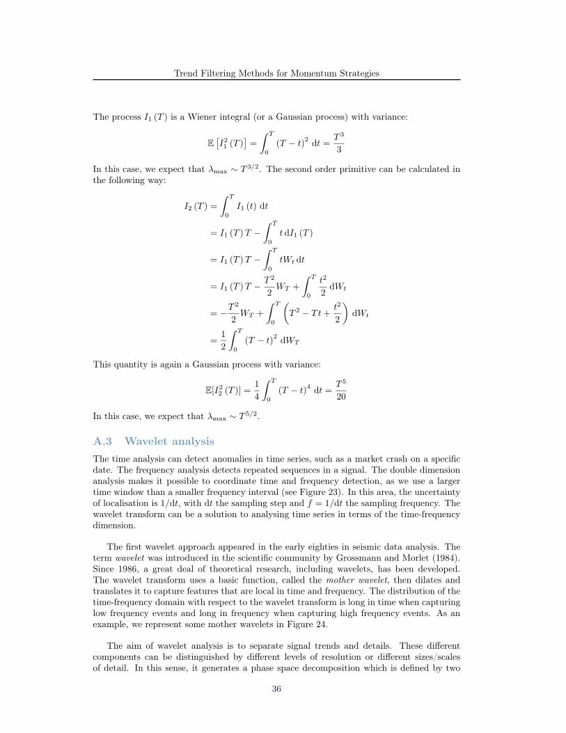
A.3 Wavelet analysisThe time analysis can detect anomalies in time series, such as a market crash on a specificdate. The frequency analysis detects repeated sequences in a signal. The double dimensionanalysis makes it possible to coordinate time and frequency detection, as we use a largertime window than a smaller frequency interval (see Figure 23). In this area, the uncertaintyof localisation is 1/dt, with dt the sampling step and f = 1/dt the sampling frequency. Thewavelet transform can be a solution to analysing time series in terms of the time-frequencydimension.

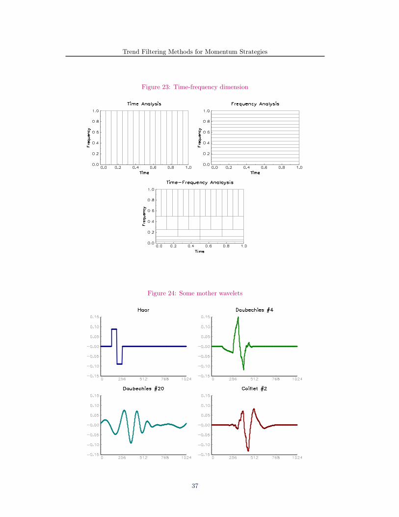
The first wavelet approach appeared in the early eighties in seismic data analysis. Theterm wavelet was introduced in the scientific community by Grossmann and Morlet (1984).Since 1986, a great deal of theoretical research, including wavelets, has been developed.The wavelet transform uses a basic function, called the mother wavelet, then dilates andtranslates it to capture features that are local in time and frequency. The distribution of thetime-frequency domain with respect to the wavelet transform is long in time when capturinglow frequency events and long in frequency when capturing high frequency events. As anexample, we represent some mother wavelets in Figure 24.

The aim of wavelet analysis is to separate signal trends and details. These differentcomponents can be distinguished by different levels of resolution or different sizes/scalesof detail. In this sense, it generates a phase space decomposition which is defined by two

36


Figure 23: Time-frequency dimension

Figure 24: Some mother wavelets

37


parameters (scale and location) in opposition to a Fourier decomposition. A wavelet ψ (t)is a function of time t such that: ∫ +∞

−∞ψ (t) dt = 0∫ +∞

−∞|ψ (t)|2 dt = 1

The continuous wavelet transform is a function of two variables W (u, s) and is given byprojecting the time series x (t) onto a particular wavelet ψ by:

W (u, s) =

∫ +∞

−∞x (t)ψu,s (t) dt

with:ψu,s (t) =

1√sψ

(t− u

s

)which corresponds to the mother wavelet translated by u (location parameter) and dilatedby s (scale parameter). If the wavelet satisfies the previous properties, the inverse operationmay be performed to produce the original signal from its wavelet coefficients:

x (t) =

∫ +∞

−∞

∫ +∞

−∞W (u, s)ψ (u, s) duds

The continuous wavelet transform of a time series signal x (t) gives an infinite numberof coefficients W (u, s) where u ∈ R and s ∈ R+, but many coefficients are close or equal tozero. The discrete wavelet transform can be used to decompose a signal into a finite numberof coefficients where we use s = 2−j as the scale parameter and u = k2−j as the locationparameter with j ∈ Z and k ∈ Z. Therefore ψu,s (t) becomes:

ψj,k(t) = 2j2ψ(2jt− k

)where j = 1, 2, ..., J in a J-level decomposition. The wavelet representation of a discretesignal x (t) is given by:

x (t) = s(0)ϕ (t) +

J−1∑j=0

2j−1∑k=0

d(j),kψj,k(t)

where ϕ (t) = 1 if t ∈ [0, 1] and J is the number of multi-resolution levels. Therefore,computing the wavelet transform of the discrete signal is equivalent to compute the smoothcoefficient s(0) and the detail coefficients d(j),k.

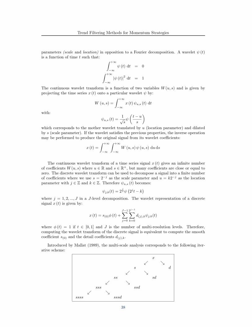
Introduced by Mallat (1989), the multi-scale analysis corresponds to the following iter-ative scheme:

x

s d

ss sd

sss ssd

ssss sssd

38


where the high-pass filter defines the details of the data and the low-pass filter defines thesmoothing signal. In this example, we obtain these wavelet coefficients:

W =

sssssssdssdsdd

Applying this pyramidal algorithm to the time series signal up to the J resolution level givesus the wavelet coefficients:

W =

s(0)d(0)d(1)...

d(J−1)

A.4 Support vector machine

The support vector machine is an important part of statistical learning theory (Hastie et al.,2009). It was first introduced by Boser et al. (1992) and has been used in various domainssuch as pattern recognition, biometrics, etc. This technique can be employed in differentcontexts such as classification, regression or density estimation (see Vapnik, 1998). Recently,applications in finance have been developed in two main directions. The first employs theSVM as a nonlinear estimator in order to forecast the trend or volatility of financial assets.In this context, the SVM is used as a regression technique with the possibility for extensionto nonlinear cases thank to the kernel approach. The second direction consists of usingthe SVM as a classification technique which aims to define the stock selection in tradingstrategies.

A.4.1 SVM in a nutshell

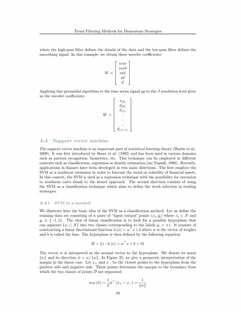
We illustrate here the basic idea of the SVM as a classification method. Let us define thetraining data set consisting of n pairs of “input/output” points (xi, yi) where xi ∈ X andyi ∈ −1, 1. The idea of linear classification is to look for a possible hyperplane thatcan separate xi ⊂ X into two classes corresponding to the labels yi = ±1. It consists ofconstructing a linear discriminant function h (x) = w⊤x+ b where w is the vector of weightsand b is called the bias. The hyperplane is then defined by the following equation:

H = x : h (x) = w⊤x+ b = 0

The vector w is interpreted as the normal vector to the hyperplane. We denote its norm∥w∥ and its direction w = w/ ∥w∥. In Figure 25, we give a geometric interpretation of themargin in the linear case. Let x+ and x− be the closest points to the hyperplane from thepositive side and negative side. These points determine the margin to the boundary fromwhich the two classes of points D are separated:

mD (h) =1

2w⊤ (x+ − x−) =

1

∥w∥

39


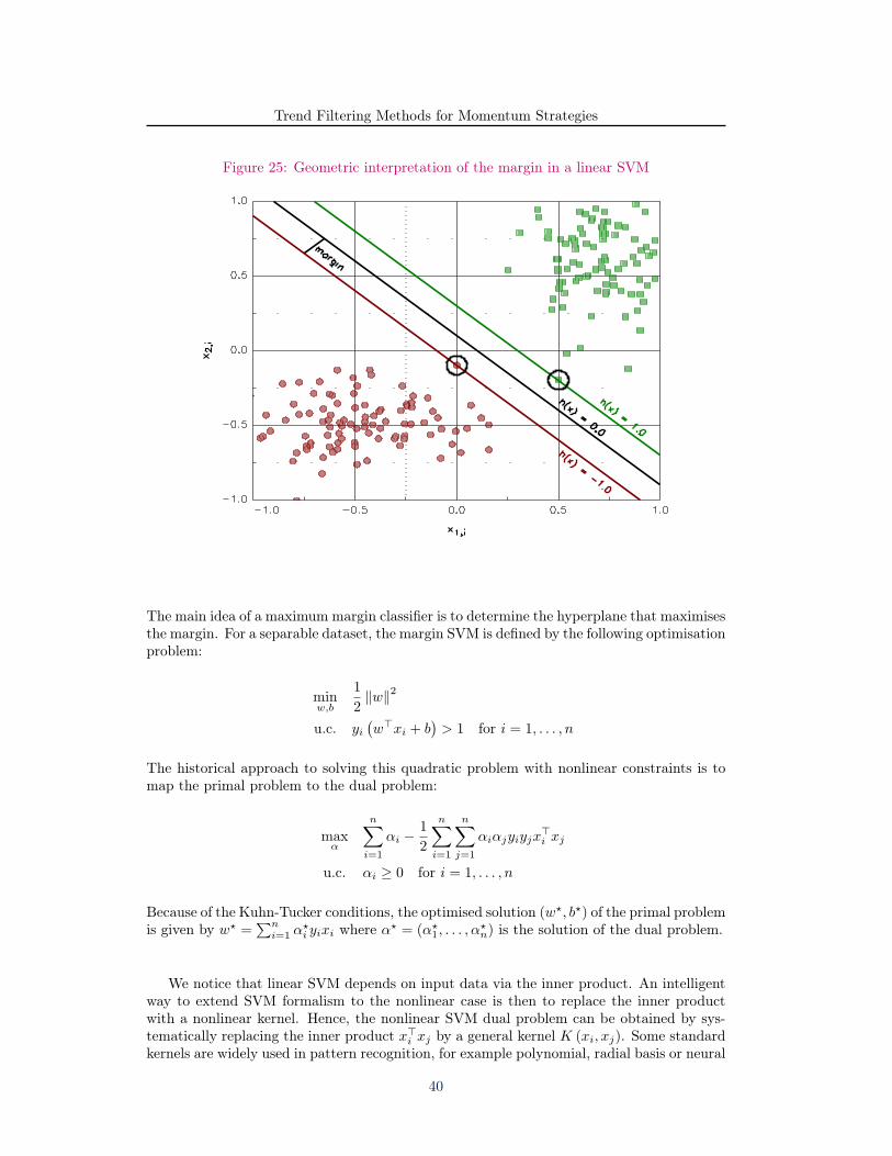
Figure 25: Geometric interpretation of the margin in a linear SVM

The main idea of a maximum margin classifier is to determine the hyperplane that maximisesthe margin. For a separable dataset, the margin SVM is defined by the following optimisationproblem:

minw,b

1

2∥w∥2

u.c. yi(w⊤xi + b

)> 1 for i = 1, . . . , n

The historical approach to solving this quadratic problem with nonlinear constraints is tomap the primal problem to the dual problem:

maxα

n∑i=1

αi −1

2

n∑i=1

n∑j=1

αiαjyiyjx⊤i xj

u.c. αi ≥ 0 for i = 1, . . . , n

Because of the Kuhn-Tucker conditions, the optimised solution (w⋆, b⋆) of the primal problemis given by w⋆ =

∑ni=1 α

⋆i yixi where α⋆ = (α⋆

1, . . . , α⋆n) is the solution of the dual problem.

We notice that linear SVM depends on input data via the inner product. An intelligentway to extend SVM formalism to the nonlinear case is then to replace the inner productwith a nonlinear kernel. Hence, the nonlinear SVM dual problem can be obtained by sys-tematically replacing the inner product x⊤i xj by a general kernel K (xi, xj). Some standardkernels are widely used in pattern recognition, for example polynomial, radial basis or neural

40


network kernels36. Finally, the decision/prediction function is then given by:

f (x) = sgnh (x) = sgn

(n∑

i=1

αiyiK (x, xi) + b

)

A.4.2 SVM regression

In the last discussion, we presented the basic idea of the SVM in the classification context.We now show how the regression problem can be interpreted as a SVM problem. In thegeneral framework of statistical learning, the SVM problem consists of minimising the riskfunction R (f) depending on the form of the prediction function f (x). The risk function iscalculated via the loss function L (f (x) , y) which clearly defines our objective (classificationor regression):

R (f) =

∫L (f (x) , y) dP (x, y)

where the distribution P (x, y) can be computed by empirical distribution37 or an approx-imated distribution38. For the regression problem, the loss function is simply defined asL (f (x) , y) = (f (x)− y)

2 or L (f (x) , y) = |f (x)− y|p in the case of Lp norm.

We have seen that the linear SVM is a special case of nonlinear SVM within the kernelapproach. We therefore consider the nonlinear case directly where the approximate functionof the regression has the following form f (x) = w⊤ϕ (x) + b. In the VRM framework, weassume that P (x, y) is a Gaussian noise with variance σ2:

R (f) =1

n

n∑i=1

|f (xi)− yi|p + σ2 ∥w∥2

We introduce the variable ξ = (ξ1, . . . , ξn) which satisfies yi = f (xi) + ξi. The optimisa-tion problem of the risk function can now be written as a QP programme with nonlinearconstraints:

minw,b,ξ

1

2∥w∥2 +

(2nσ2

)−1n∑

i=1

|ξi|p

u.c. yi = w⊤ϕ (xi) + b+ ξi for i = 1, . . . , n

In the present form, the regression looks very similar to the SVM classification problem andcan be solved in the same way by mapping to the dual problem. We notice that the SVMregression can be easily generalised in two possible ways:

1. by introducing a more general loss function such as the ε-SV regression proposed byVapnik (1998);

2. by using a weighting distribution ω for the empirical distribution:

dP (x, y) =

n∑i=1

ωiδxi (x) δyi (y)

36We have, respectively, K (xi, xj) =(x⊤i xj + 1

)p, K (xi, xj) = exp(−∥xi − xj∥2 /

(2σ2

))or

K (xi, xj) = tanh(ax⊤

i xj − b).

37This framework called ERM was first introduced by Vapnik and Chervonenskis (1991).38This framework is called VRM (Chapelle, 2002).

41


As financial series have short memory and depend more on the recent past, an asym-metric weight distribution focusing on recent data would improve the prediction39.

The dual problem in the case p = 1 is given by:

maxα

α⊤y − 1

2α⊤Kα

u.c.α⊤1 = 0

|α| ≤(2nσ2

)−11

As previously, the optimal vector α⋆ is obtained by solving the QP programme. We thendeduce that w⋆ =

∑ni=1 α

⋆i ϕ (xi) and b⋆ is computed using the Kuhn-Tucker condition:

w⊤ϕ (xi) + b− yi = 0

for support vectors (xi, yi). In order to achieve a good level of accuracy for the estimationof b, we average out the set of support vectors and obtain b⋆. The SVM regressor is thengiven by the following formula:

f (x) =n∑

i=1

α⋆iK (x, xi) + b⋆

with K (x, xi) = ϕ (x)ϕ (xi).

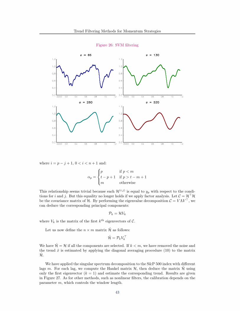
In Figure 26, we apply SVM regression with the Gaussian kernel to the S&P 500 index.The kernel parameter σ characterises the estimation horizon which is equivalent to periodn in the moving average regression.

A.5 Singular spectrum analysis

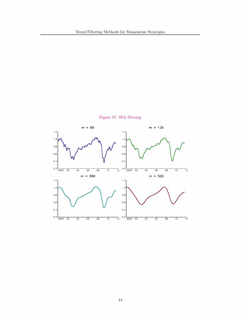
In recent years the singular spectrum analysis (SSA) technique has been developed as atime-frequency domain method40. It consists of decomposing a time series into a trend,oscillatory components and a noise.

The method is based on the principal component analysis of the auto-covariance matrixof the time series y = (y1, . . . , yt). Let n be the window length such that n = t−m+1 withm < t/2. We define the n ×m Hankel matrix H as the matrix of the m concatenated lagvector of y:

H =

y1 y2 y3 · · · ymy2 y3 y4 · · · ym+1

y3 y4 y5 · · ·...

......

.... . . yt−1

yn yn+1 yn+2 · · · yt

We recover the time series y by diagonal averaging:

yp =1

αp

m∑j=1

H(i,j) (10)

39See Gestel et al. (2001) and Tay and Cao 2002.40Introduced by Broomhead and King (1986).

42


Figure 26: SVM filtering

where i = p− j + 1, 0 < i < n+ 1 and:

αp =

p if p < m

t− p+ 1 if p > t−m+ 1

m otherwise

This relationship seems trivial because each H(i,j) is equal to yp with respect to the condi-tions for i and j. But this equality no longer holds if we apply factor analysis. Let C = H⊤Hbe the covariance matrix of H. By performing the eigenvalue decomposition C = V ΛV ⊤, wecan deduce the corresponding principal components:

Pk = HVk

where Vk is the matrix of the first kth eigenvectors of C.

Let us now define the n×m matrix H as follows:

H = PkV⊤k

We have H = H if all the components are selected. If k < m, we have removed the noise andthe trend x is estimated by applying the diagonal averaging procedure (10) to the matrixH.

We have applied the singular spectrum decomposition to the S&P 500 index with differentlags m. For each lag, we compute the Hankel matrix H, then deduce the matrix H usingonly the first eigenvector (k = 1) and estimate the corresponding trend. Results are givenin Figure 27. As for other methods, such as nonlinear filters, the calibration depends on theparameter m, which controls the window length.

43


Figure 27: SSA filtering

44


References[1] Alexandrov T., Bianconcini S., Dagum E.B., Maass P. and McElroy T. (2008),

A Review of Some Modern Approaches to the Problem of Trend Extraction , US CensusBureau, RRS #2008/03.

[2] Antoniadis A., Gregoire G. and McKeague I.W. (1994), Wavelet Methods forCurve Estimation, Journal of the American Statistical Association, 89(428), pp. 1340-1353.

[3] Barberis N. and Thaler T. (2002), A Survey of Behavioral Finance, NBER WorkingPaper, 9222.

[4] Beveridge S. and Nelson C.R. (1981), A New Approach to the Decomposition ofEconomic Time Series into Permanent and Transitory Components with ParticularAttention to Measurement of the Business Cycle, Journal of Monetary Economics,7(2), pp. 151-174.

[5] Boser B.E., Guyon I.M. and Vapnik V. (1992), A Training Algorithm for OptimalMargin Classifier, Proceedings of the Fifth Annual Workshop on Computational Learn-ing Theory, pp. 114-152.

[6] Boyd S. and Vandenberghe L. (2009), Convex Optimization, Cambridge UniversityPress.

[7] Brockwell P.J. and Davis R.A. (2003), Introduction to Time Series and Forecasting,Springer.

[8] Broomhead D.S. and King G.P. (1986), On the Qualitative Analysis of ExperimentalDynamical Systems, in Sarkar S. (ed.), Nonlinear Phenomena and Chaos, Adam Hilger,pp. 113-144.

[9] Brown S.J., Goetzmann W.N. and Kumar A. (1998), The Dow Theory: WilliamPeter Hamilton’s Track Record Reconsidered, Journal of Finance, 53(4), pp. 1311-1333.

[10] Burch N., Fishback P.E. and Gordon R. (2005), The Least-Squares Property of theLanczos Derivative, Mathematics Magazine, 78(5), pp. 368-378.

[11] Carhart M.M. (1997), On Persistence in Mutual Fund Performance, Journal of Fi-nance, 52(1), pp. 57-82.

[12] Chan L.K.C., Jegadeesh N. and Lakonishok J. (1996), Momentum Strategies, Jour-nal of Finance, 51(5), pp. 1681-1713.

[13] Chang Y., Miller J.I. and Park J.Y. (2009), Extracting a Common Stochastic Trend:Theory with Some Applications, Journal of Econometrics, 150(2), pp. 231-247.

[14] Chapelle O. (2002), Support Vector Machine: Induction Principles, Adaptive Tuningand Prior Knowledge, PhD thesis, University of Paris 6.

[15] Cleveland W.P. and Tiao G.C. (1976), Decomposition of Seasonal Time Series: AModel for the Census X-11 Program, Journal of the American Statistical Association,71(355), pp. 581-587.

[16] Cleveland W.S. (1979), Robust Locally Regression and Smoothing Scatterplots, Jour-nal of the American Statistical Association, 74(368), pp. 829-836.

45


[17] Cleveland W.S. and Devlin S.J. (1988), Locally Weighted Regression: An Approachto Regression Analysis by Local Fitting, Journal of the American Statistical Associa-tion, 83(403), pp. 596-610.

[18] Cochrane J. (2001), Asset Pricing, Princeton University Press.

[19] Cortes C. and Vapnik V. (1995), Support-Vector Networks, Machine Learning, 20(3),pp. 273-297.

[20] D’Aspremont A. (2011), Identifying Small Mean Reverting Portfolios, QuantitativeFinance, 11(3), pp. 351-364.

[21] Daubechies I. (1992), Ten Lectures on Wavelets, SIAM.

[22] Daubechies I., Defrise M. and De Mol C. (2004), An Iterative Thresholding Al-gorithm for Linear Inverse Problems with a Sparsity Constraint, Communications onPure and Applied Mathematics, 57(11), pp. 1413-1457.

[23] Donoho D.L. (1995), De-Noising by Soft-Thresholding, IEEE Transactions on Infor-mation Theory, 41(3), pp. 613-627.

[24] Donoho D.L. and Johnstone I.M. (1994), Ideal Spatial Adaptation via WaveletShrinkage, Biometrika, 81(3), pp. 425-455.

[25] Donoho D.L. and Johnstone I.M. (1995), Adapting to Unknown Smoothness viaWavelet Shrinkage, Journal of the American Statistical Association, 90(432), pp. 1200-1224.

[26] Doucet A., De Freitas N. and Gordon N. (2001), Sequential Monte Carlo in Prac-tice, Springer.

[27] Ehlers J.F. (2001), Rocket Science for Traders: Digital Signal Processing Applications,John Wiley & Sons.

[28] Elton E.J. and Gruber M.J. (1972), Earnings Estimates and the Accuracy of Expec-tational Data, Management Science, 18(8), pp. 409-424.

[29] Engle R.F. and Granger C.W.J. (1987), Co-Integration and Error Correction: Rep-resentation, Estimation, and Testing, Econometrica, 55(2), pp. 251-276.

[30] Fama E. (1970), Efficient Capital Markets: A Review of Theory and Empirical Work,Journal of Finance, 25(2), pp. 383-417.

[31] Flandrin P., Rilling G. and Goncalves P. (2004), Empirical Mode Decompositionas a Filter Bank, Signal Processing Letters, 11(2), pp. 112-114.

[32] Fliess M. and Join C. (2009), A Mathematical Proof of the Existence of Trends inFinancial Time Series, in El Jai A., Afifi L. and Zerrik E. (eds), Systems Theory:Modeling, Analysis and Control, Presses Universitaires de Perpignan, pp. 43-62.

[33] Fuentes M. (2002), Spectral Methods for Nonstationary Spatial Processes, Biometrika,89(1), pp. 197-210.

[34] Gençay R., Selçuk F. and Whitcher B. (2002), An Introduction to Wavelets andOther Filtering Methods in Finance and Economics, Academic Press.

46


[35] Gestel T.V., Suykens J.A.K., Baestaens D., Lambrechts A., Lanckriet G.,Vandaele B., De Moor B. and Vandewalle J. (2001), Financial Time Series Pre-diction Using Least Squares Support Vector Machines Within the Evidence Framework,IEEE Transactions on Neural Networks, 12(4), pp. 809-821.

[36] Golyandina N., Nekrutkin V.V. and Zhigljavsky A.A. (2001), Analysis of TimeSeries Structure: SSA and Related Techniques, Chapman & Hall, CRC.

[37] Gonzalo J. and Granger C.W.J. (1995), Estimation of Common Long-Memory Com-ponents in Cointegrated Systems, Journal of Business & Economic Statistics, 13(1), pp.27-35.

[38] Grinblatt M., Titman S. and Wermers R. (1995), Momentum Investment Strate-gies, Portfolio Performance, and Herding: A Study of Mutual Fund Behavior, AmericanEconomic Review, 85(5), pp. 1088-1105.

[39] Groetsch C.W. (1998), Lanczo’s Generalized Derivative, American MathematicalMonthly, 105(4), pp. 320-326.

[40] Grossmann A. and Morlet J. (1984), Decomposition of Hardy Functions into SquareIntegrable Wavelets of Constant Shape, SIAM Journal of Mathematical Analysis, 15,pp. 723-736.

[41] Härdle W. (1992), Applied Nonparametric Regression, Cambridge University Press.

[42] Harvey A.C. (1989), Forecasting, Structural Time Series Models and the Kalman Fil-ter, Cambridge University Press.

[43] Harvey A.C. and Trimbur T.M. (2003), General Model-Based Filters for ExtractingCycles and Trends in Economic Time Series, Review of Economics and Statistics, 85(2),pp. 244-255.

[44] Hastie T., Tibshirani R. and Friedman R. (2009), The Elements of Statistical Learn-ing, second edition, Springer.

[45] Henderson R. (1916), Note on Graduation by Adjusted Average, Transactions of theActuarial Society of America, 17, pp. 43-48.

[46] Hodrick R.J. and Prescott E.C. (1997), Postwar U.S. Business Cycles: An EmpiricalInvestigation, Journal of Money, Credit and Banking, 29(1), pp. 1-16.

[47] Holt C.C. (1959), Forecasting Seasonals and Trends by Exponentially Weighted Mov-ing Averages, ONR Research Memorandum, 52, reprinted in International Journal ofForecasting, 2004, 20(1), pp. 5-10.

[48] Hong H. and Stein J.C. (1977), A Unified Theory of Underreaction, Momentum Trad-ing and Overreaction in Asset Markets, NBER Working Paper, 6324.

[49] Johansen S. (1988), Statistical Analysis of Cointegration Vectors, Journal of EconomicDynamics and Control, 12(2-3), pp. 231-254.

[50] Johansen S. (1991), Estimation and Hypothesis Testing of Cointegration Vectors inGaussian Vector Autoregressive Models, Econometrica, 52(6), pp. 1551-1580.

[51] Kalaba R. and Tesfatsion L. (1989), Time-varying Linear Regression via FlexibleLeast Squares, Computers & Mathematics with Applications, 17, pp. 1215-1245.

47


[52] Kalman R.E. (1960), A New Approach to Linear Filtering and Prediction Problems,Transactions of the ASME – Journal of Basic Engineering, 82(D), pp. 35-45.

[53] Kendall M.G. (1973), Time Series, Charles Griffin.

[54] Kim S-J., Koh K., Boyd S. and Gorinevsky D. (2009), ℓ1 Trend Filtering, SIAMReview, 51(2), pp. 339-360.

[55] Kolmogorov A.N. (1941), Interpolation and Extrapolation of Random Sequences,Izvestiya Akademii Nauk SSSR, Seriya Matematicheskaya, 5(1), pp. 3-14.

[56] Macaulay F. (1931), The Smoothing of Time Series, National Bureau of EconomicResearch.

[57] Mallat S.G. (1989), A Theory for Multiresolution Signal Decomposition: The WaveletRepresentation, IEEE Transactions on Pattern Analysis and Machine Intelligence,11(7), pp. 674-693.

[58] Mann H.B. (1945), Nonparametric Tests against Trend, Econometrica, 13(3), pp. 245-259.

[59] Martin W. and Flandrin P. (1985), Wigner-Ville Spectral Analysis of NonstationaryProcesses, IEEE Transactions on Acoustics, Speech and Signal Processing, 33(6), pp.1461-1470.

[60] Muth J.F. (1960), Optimal Properties of Exponentially Weighted Forecasts, Journalof the American Statistical Association, 55(290), pp. 299-306.

[61] Oppenheim A.V. and Schafer R.W. (2009), Discrete-Time Signal Processing, thirdedition, Prentice-Hall.

[62] Peña D. and Box, G.E.P. (1987), Identifying a Simplifying Structure in Time Series,Journal of the American Statistical Association, 82(399), pp. 836-843.

[63] Pollock, D.S.G. (2006), Wiener-Kolmogorov Filtering Frequency-Selective Filteringand Polynomial Regression, Econometric Theory, 23, pp. 71-83.

[64] Pollock D.S.G. (2009), Statistical Signal Extraction: A Partial Survey, in Kon-toghiorges E. and Belsley D.E. (eds.), Handbook of Empirical Econometrics, John Wileyand Sons.

[65] Rao S.T. and Zurbenko I.G. (1994), Detecting and Tracking Changes in Ozone airQuality, Journal of Air and Waste Management Association, 44(9), pp. 1089-1092.

[66] Roncalli T. (2010), La Gestion d’Actifs Quantitative, Economica.

[67] Savitzky A. and Golay M.J.E. (1964), Smoothing and Differentiation of Data bySimplified Least Squares Procedures, Analytical Chemistry, 36(8), pp. 1627-1639.

[68] Silverman B.W. (1985), Some Aspects of the Spline Smoothing Approach to Non-Parametric Regression Curve Fitting, Journal of the Royal Statistical Society, B47(1),pp. 1-52.

[69] Sorenson H.W. (1970), Least-Squares Estimation: From Gauss to Kalman, IEEESpectrum, 7, pp. 63-68.

48


[70] Stock J.H. and Watson M.W. (1988), Variable Trends in Economic Time Series,Journal of Economic Perspectives, 2(3), pp. 147-174.

[71] Tay F.E.H. and Cao L.J. (2002), Modified Support Vector Machines in Financial TimesSeries Forecasting, Neurocomputing, 48(1-4), pp. 847-861.

[72] Tibshirani R. (1996), Regression Shrinkage and Selection via the Lasso, Journal ofthe Royal Statistical Society, B58(1), pp. 267-288.

[73] Vapnik V. (1998), Statistical Learning Theory, John Wiley and Sons, New York.

[74] Vapnik V. and Chervonenskis A. (1991), On the Uniform Convergence of RelativeFrequency of Events to their Probabilities, Theory of Probability and its Applications,16(2), pp. 264-280.

[75] Vautard R., Yiou P., and Ghil M. (1992), Singular Spectrum Analysis: A Toolkitfor Short, Noisy Chaotic Signals, Physica D, 58(1-4), pp. 95-126.

[76] Wahba G. (1990), Spline Models for Observational Data, CBMS-NSF Regional Con-ference Series in Applied Mathematics, 59, SIAM.

[77] Wang Y. (1998), Change Curve Estimation via Wavelets, Journal of the AmericanStatistical Association, 93(441), pp. 163-172.

[78] Wiener N. (1949), Extrapolation, Interpolation and Smoothing of Stationary TimeSeries with Engineering Applications, MIT Technology Press and John Wiley & Sons(originally published in 1941 as a Report on the Services Research Project, DIC-6037).

[79] Whittaker E.T. (1923), On a New Method of Graduation, Proceedings of the Edin-burgh Mathematical Society, 41, pp. 63-75.

[80] Winters P.R. (1960), Forecasting Sales by Exponentially Weighted Moving Averages,Management Science, 6(3), 324-342.

[81] Yue S. and Pilon P. (2004), A Comparison of the Power of the t-test, Mann-Kendalland Bootstrap Tests for Trend Detection, Hydrological Sciences Journal, 49(1), 21-37.

[82] Zurbenko I., Porter P.S., Rao S.T., Ku J.K., Gui R. and Eskridge R.E. (1996),Detecting Discontinuities in Time Series of Upper-Air Data: Demonstration of an Adap-tive Filter Technique, Journal of Climate, 9(12), pp. 3548-3560.

49

Documents

Trend Filtering Methods for Momentum Strategiesthierry-roncalli.com/download/lwp-tf.pdf · 1. the trend following strategy, ... in trading strategies. ... Trend Filtering Methods