Section 2.1

Tree Diagrams

Example 2.1 Problem

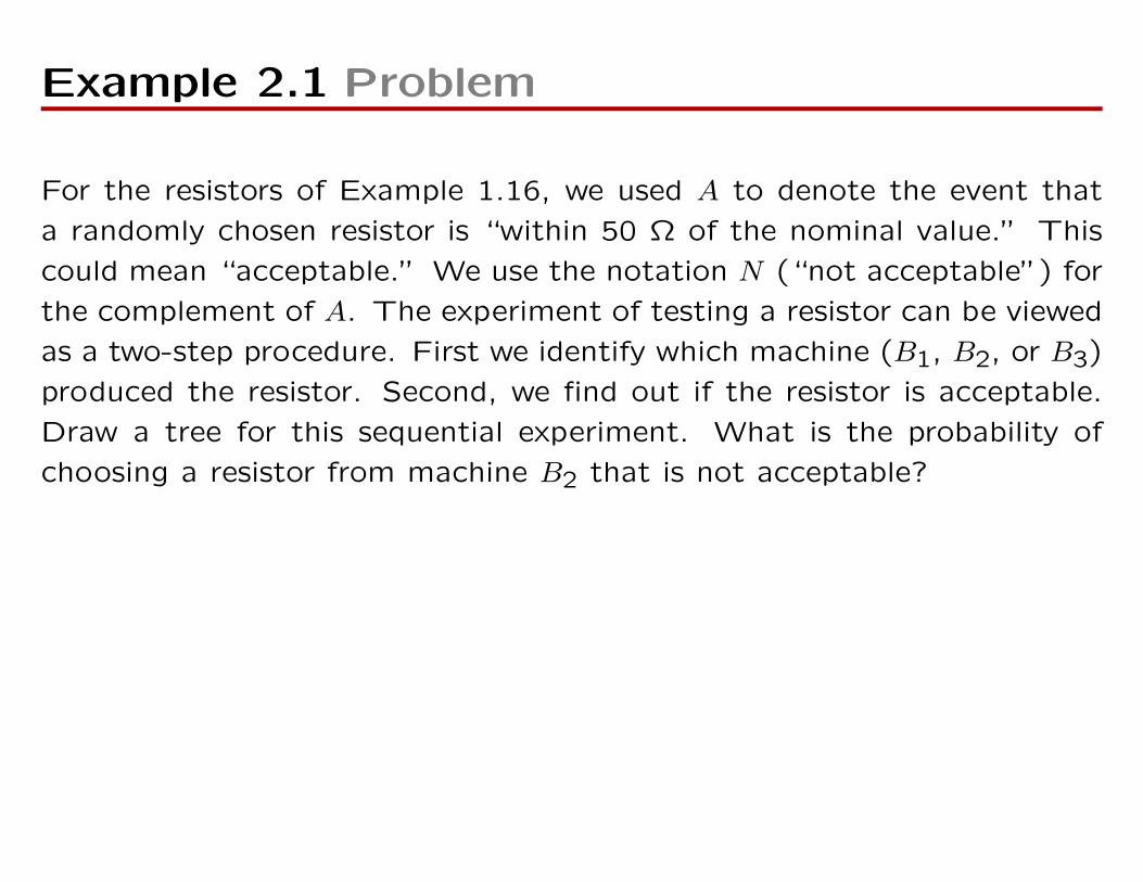
For the resistors of Example 1.16, we used A to denote the event that

a randomly chosen resistor is “within 50 Ω of the nominal value.” This

could mean “acceptable.” We use the notation N (“not acceptable”) for

the complement of A. The experiment of testing a resistor can be viewed

as a two-step procedure. First we identify which machine (B1, B2, or B3)

produced the resistor. Second, we find out if the resistor is acceptable.

Draw a tree for this sequential experiment. What is the probability of

choosing a resistor from machine B2 that is not acceptable?

Example 2.1 Solution

B20.4

B10.3

HHHHHH

HH B30.3

A0.8N0.2

A0.9XXXXXXXX N0.1

A0.6XXXXXXXX N0.4

•B1A 0.24•B1N 0.06•B2A 0.36

•B2N 0.04•B3A 0.18•B3N 0.12

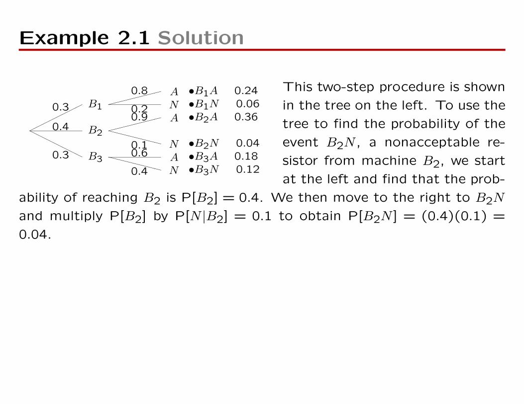
This two-step procedure is shown

in the tree on the left. To use the

tree to find the probability of the

event B2N , a nonacceptable re-

sistor from machine B2, we start

at the left and find that the prob-

ability of reaching B2 is P[B2] = 0.4. We then move to the right to B2N

and multiply P[B2] by P[N |B2] = 0.1 to obtain P[B2N ] = (0.4)(0.1) =

0.04.

Example 2.2 Problem

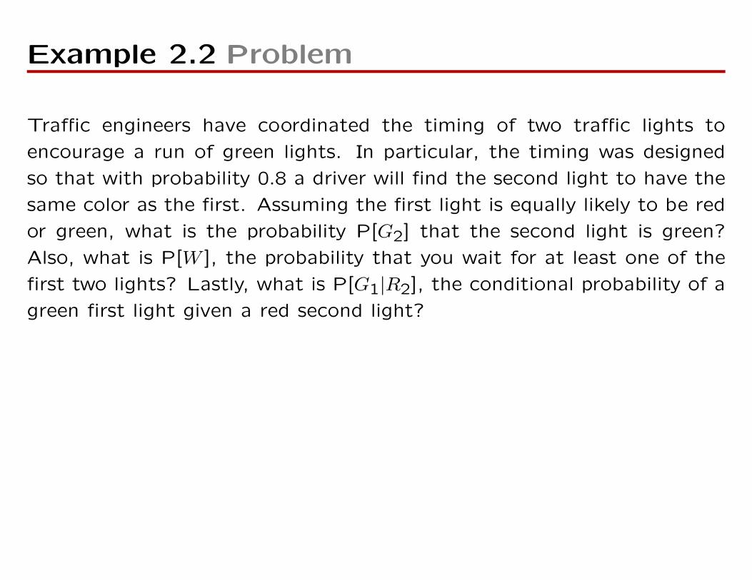
Traffic engineers have coordinated the timing of two traffic lights to

encourage a run of green lights. In particular, the timing was designed

so that with probability 0.8 a driver will find the second light to have the

same color as the first. Assuming the first light is equally likely to be red

or green, what is the probability P[G2] that the second light is green?

Also, what is P[W ], the probability that you wait for at least one of the

first two lights? Lastly, what is P[G1|R2], the conditional probability of a

green first light given a red second light?

Example 2.2 Solution

G10.5

HHHHHH

HHHHR10.5

G20.8

XXXXXXXXXXR20.2

G20.2

XXXXXXXXXXR20.8

•G1G2 0.4

•G1R2 0.1

•R1G2 0.1

•R1R2 0.4

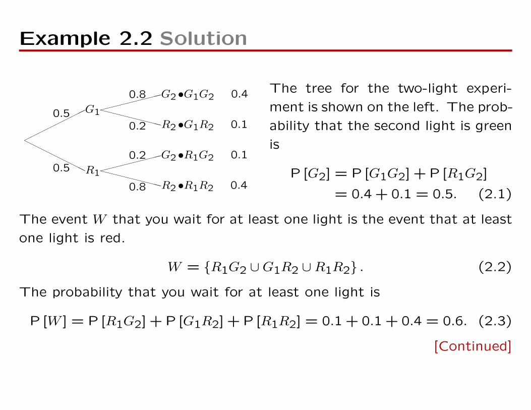
The tree for the two-light experi-

ment is shown on the left. The prob-

ability that the second light is green

is

P [G2] = P [G1G2] + P [R1G2]

= 0.4 + 0.1 = 0.5. (2.1)

The event W that you wait for at least one light is the event that at least

one light is red.

W = R1G2 ∪G1R2 ∪R1R2 . (2.2)

The probability that you wait for at least one light is

P [W ] = P [R1G2] + P [G1R2] + P [R1R2] = 0.1 + 0.1 + 0.4 = 0.6. (2.3)

[Continued]

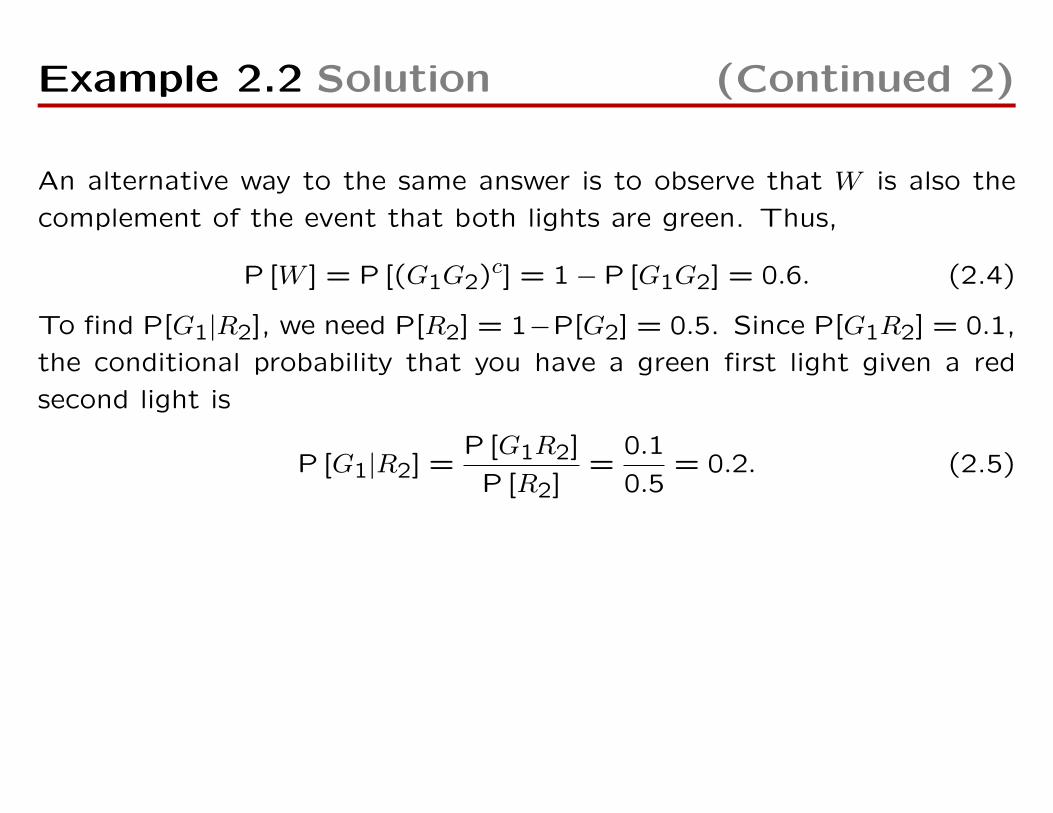
Example 2.2 Solution (Continued 2)

An alternative way to the same answer is to observe that W is also the

complement of the event that both lights are green. Thus,

P [W ] = P [(G1G2)c] = 1− P [G1G2] = 0.6. (2.4)

To find P[G1|R2], we need P[R2] = 1−P[G2] = 0.5. Since P[G1R2] = 0.1,

the conditional probability that you have a green first light given a red

second light is

P [G1|R2] =P [G1R2]

P [R2]=

0.1

0.5= 0.2. (2.5)

Example 2.3 Problem

In the Monty Hall game, a new car is hidden behind one of three closed doors while agoat is hidden behind each of the other two doors. Your goal is to select the door thathides the car. You make a preliminary selection and then a final selection. The gameproceeds as follows:

• You select a door.

• The host, Monty Hall (who knows where the car is hidden), opens one of the twodoors you didn’t select to reveal a goat.

• Monty then asks you if you would like to switch your selection to the other unopeneddoor.

• After you make your choice (either staying with your original door, or switchingdoors), Monty reveals the prize behind your chosen door.

To maximize your probability P[C] of winning the car, is switching to the other dooreither (a) a good idea, (b) a bad idea or (c) makes no difference?

Example 2.3 Solution

To solve this problem, we will consider the “switch” and “do not switch” policiesseparately. That is, we will construct two different tree diagrams: The first describeswhat happens if you switch doors while the second describes what happens if you donot switch.

First we describe what is the same no matter what policy you follow. Suppose the doorsare numbered 1, 2, and 3. Let Hi denote the event that the car is hidden behind doori. Also, let’s assume you first choose door 1. (Whatever door you do choose, that doorcan be labeled door 1 and it would not change your probability of winning.) Now let Ridenote the event that Monty opens door i that hides a goat. If the car is behind door1 Monty can choose to open door 2 or door 3 because both hide goats. He choosesdoor 2 or door 3 by flipping a fair coin. If the car is behind door 2, Monty opens door 3and if the car is behind door 3, Monty opens door 2. Let C denote the event that youwin the car and G the event that you win a goat. After Monty opens one of the doors,you decide whether to change your choice or stay with your choice of door 1. Finally,Monty opens the door of your final choice, either door 1 or the door you switched to.

[Continued]

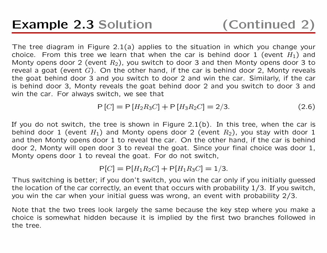
Example 2.3 Solution (Continued 2)

The tree diagram in Figure 2.1(a) applies to the situation in which you change yourchoice. From this tree we learn that when the car is behind door 1 (event H1) andMonty opens door 2 (event R2), you switch to door 3 and then Monty opens door 3 toreveal a goat (event G). On the other hand, if the car is behind door 2, Monty revealsthe goat behind door 3 and you switch to door 2 and win the car. Similarly, if the caris behind door 3, Monty reveals the goat behind door 2 and you switch to door 3 andwin the car. For always switch, we see that

P [C] = P [H2R3C] + P [H3R2C] = 2/3. (2.6)

If you do not switch, the tree is shown in Figure 2.1(b). In this tree, when the car isbehind door 1 (event H1) and Monty opens door 2 (event R2), you stay with door 1and then Monty opens door 1 to reveal the car. On the other hand, if the car is behinddoor 2, Monty will open door 3 to reveal the goat. Since your final choice was door 1,Monty opens door 1 to reveal the goat. For do not switch,

P[C] = P[H1R2C] + P[H1R3C] = 1/3.

Thus switching is better; if you don’t switch, you win the car only if you initially guessedthe location of the car correctly, an event that occurs with probability 1/3. If you switch,you win the car when your initial guess was wrong, an event with probability 2/3.

Note that the two trees look largely the same because the key step where you make achoice is somewhat hidden because it is implied by the first two branches followed inthe tree.

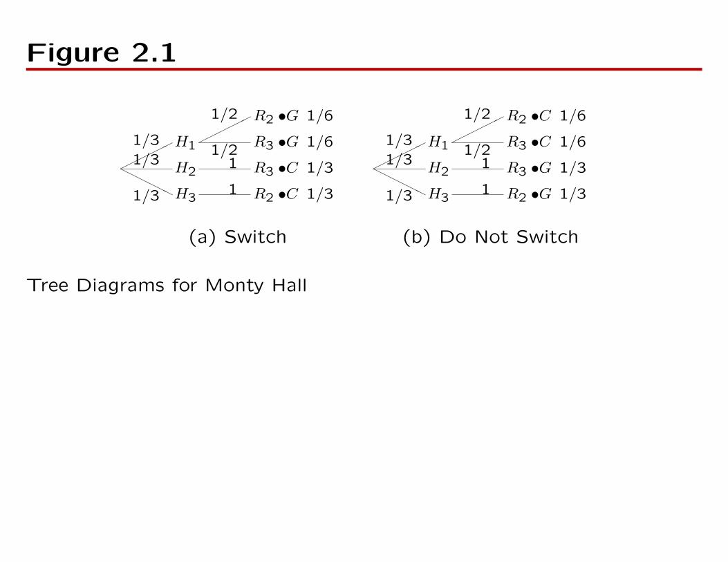
Figure 2.1

H21/3

H11/3

HHHHHHH31/3

R21/2

R31/2R3

1

R21

•G 1/6

•G 1/6

•C 1/3

•C 1/3

H21/3

H11/3

HHHHHHH31/3

R21/2

R31/2R3

1

R21

•C 1/6

•C 1/6

•G 1/3

•G 1/3

(a) Switch (b) Do Not Switch

Tree Diagrams for Monty Hall

Quiz 2.1

In a cellular phone system, a mobile phone must be paged to receive a

phone call. However, paging attempts don’t always succeed because the

mobile phone may not receive the paging signal clearly. Consequently,

the system will page a phone up to three times before giving up. If the

results of all paging attempts are independent and a single paging attempt

succeeds with probability 0.8, sketch a probability tree for this experiment

and find the probability P[F ] that the phone receives the paging signal

clearly.

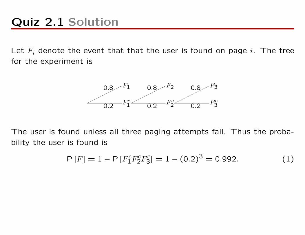
Quiz 2.1 Solution

Let Fi denote the event that that the user is found on page i. The tree

for the experiment is

F10.8

F c10.2

F20.8

F c20.2

F30.8

F c30.2

The user is found unless all three paging attempts fail. Thus the proba-

bility the user is found is

P [F ] = 1− P [F c1Fc2F

c3] = 1− (0.2)3 = 0.992. (1)

Section 2.2

Counting Methods

Example 2.4 Problem

Choose 7 cards at random from a deck of 52 different cards. Display

the cards in the order in which you choose them. How many different

sequences of cards are possible?

Example 2.4 Solution

The procedure consists of seven subexperiments. In each subexperiment,

the observation is the identity of one card. The first subexperiment has 52

possible outcomes corresponding to the 52 cards that could be drawn. For

each outcome of the first subexperiment, the second subexperiment has

51 possible outcomes corresponding to the 51 remaining cards. Therefore

there are 52 × 51 outcomes of the first two subexperiments. The total

number of outcomes of the seven subexperiments is

52× 51× · · · × 46 = 674,274,182,400 . (2.7)

Theorem 2.1

Fundamental Principle of

Counting

An experiment consists of two subexperiments. If one subexperiment

has k outcomes and the other subexperiment has n outcomes, then the

experiment has nk outcomes.

Example 2.5

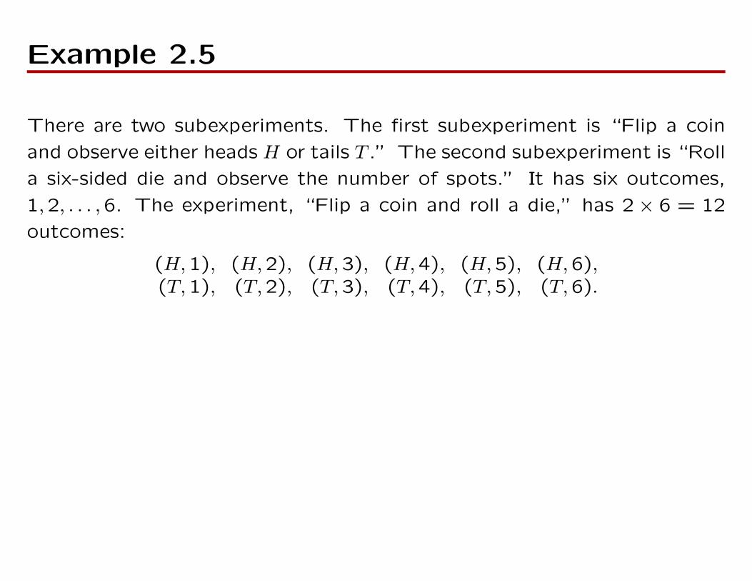
There are two subexperiments. The first subexperiment is “Flip a coin

and observe either heads H or tails T .” The second subexperiment is “Roll

a six-sided die and observe the number of spots.” It has six outcomes,

1,2, . . . ,6. The experiment, “Flip a coin and roll a die,” has 2 × 6 = 12

outcomes:

(H,1), (H,2), (H,3), (H,4), (H,5), (H,6),(T,1), (T,2), (T,3), (T,4), (T,5), (T,6).

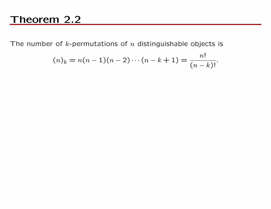
Theorem 2.2

The number of k-permutations of n distinguishable objects is

(n)k = n(n− 1)(n− 2) · · · (n− k + 1) =n!

(n− k)!.

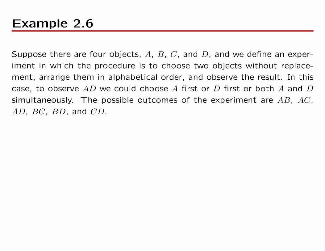
Example 2.6

Suppose there are four objects, A, B, C, and D, and we define an exper-

iment in which the procedure is to choose two objects without replace-

ment, arrange them in alphabetical order, and observe the result. In this

case, to observe AD we could choose A first or D first or both A and D

simultaneously. The possible outcomes of the experiment are AB, AC,

AD, BC, BD, and CD.

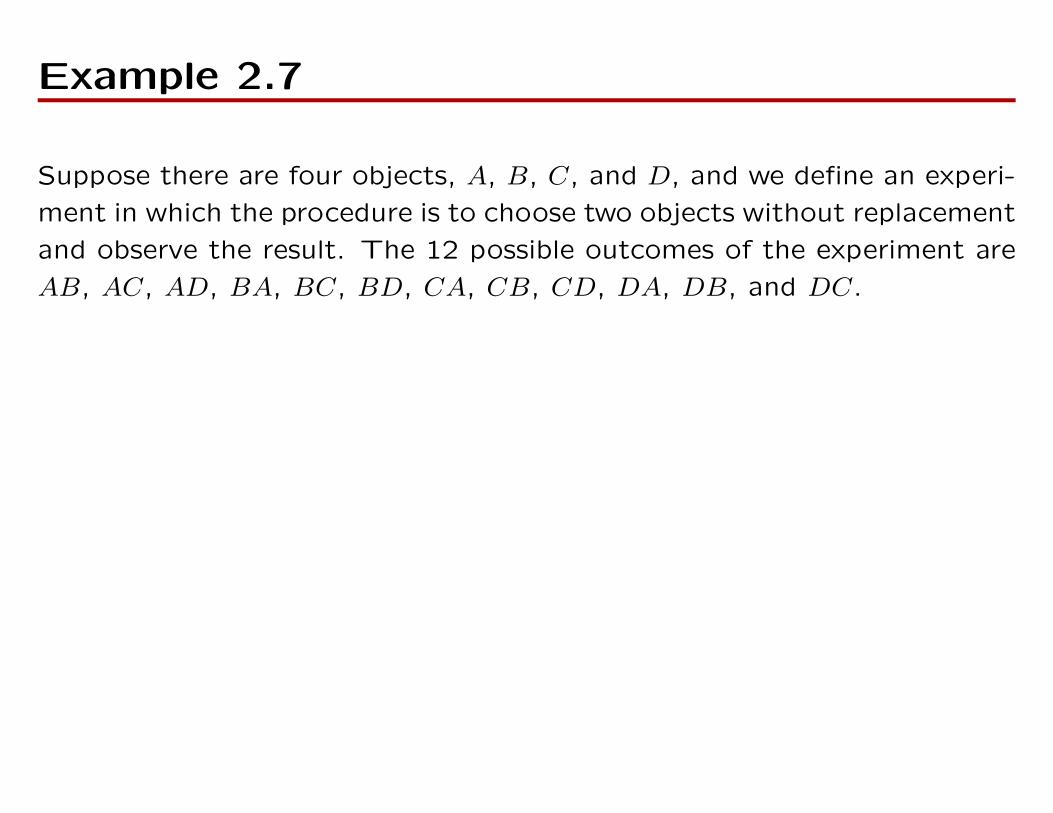
Example 2.7

Suppose there are four objects, A, B, C, and D, and we define an experi-

ment in which the procedure is to choose two objects without replacement

and observe the result. The 12 possible outcomes of the experiment are

AB, AC, AD, BA, BC, BD, CA, CB, CD, DA, DB, and DC.

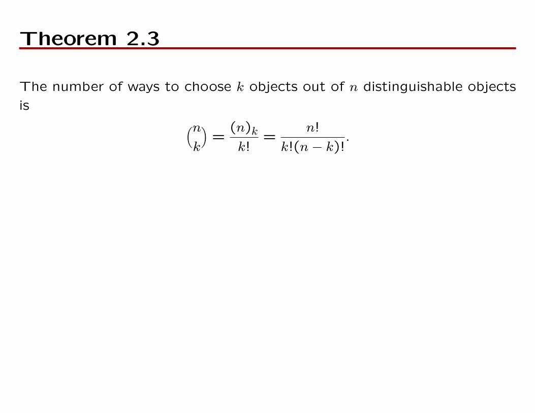
Theorem 2.3

The number of ways to choose k objects out of n distinguishable objects

is (nk

)=

(n)kk!

=n!

k!(n− k)!.

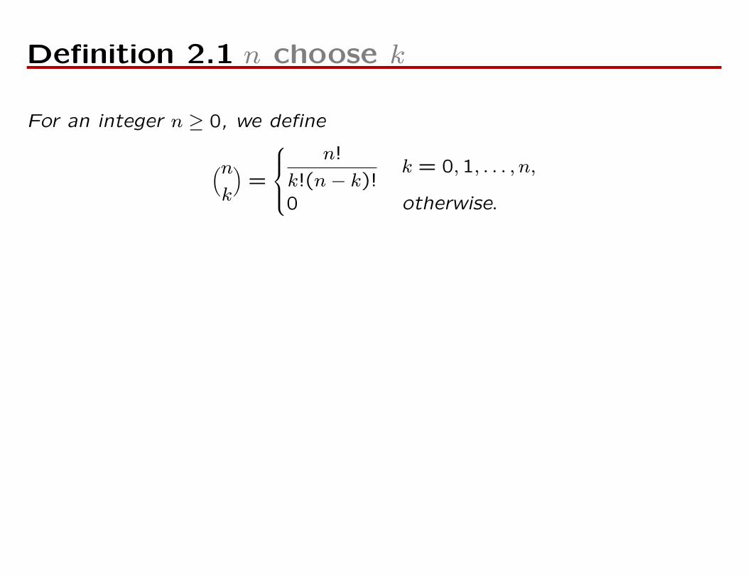
Definition 2.1 n choose k

For an integer n ≥ 0, we define

(nk

)=

n!

k!(n− k)!k = 0,1, . . . , n,

0 otherwise.

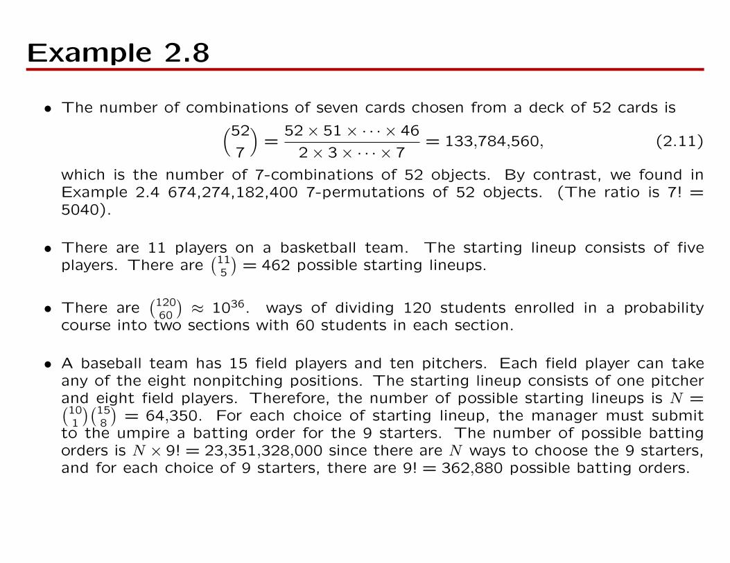
Example 2.8

• The number of combinations of seven cards chosen from a deck of 52 cards is(52

7

)=

52× 51× · · · × 46

2× 3× · · · × 7= 133,784,560, (2.11)

which is the number of 7-combinations of 52 objects. By contrast, we found inExample 2.4 674,274,182,400 7-permutations of 52 objects. (The ratio is 7! =5040).

• There are 11 players on a basketball team. The starting lineup consists of fiveplayers. There are

(115

)= 462 possible starting lineups.

• There are(120

60

)≈ 1036. ways of dividing 120 students enrolled in a probability

course into two sections with 60 students in each section.

• A baseball team has 15 field players and ten pitchers. Each field player can takeany of the eight nonpitching positions. The starting lineup consists of one pitcherand eight field players. Therefore, the number of possible starting lineups is N =(10

1

)(158

)= 64,350. For each choice of starting lineup, the manager must submit

to the umpire a batting order for the 9 starters. The number of possible battingorders is N × 9! = 23,351,328,000 since there are N ways to choose the 9 starters,and for each choice of 9 starters, there are 9! = 362,880 possible batting orders.

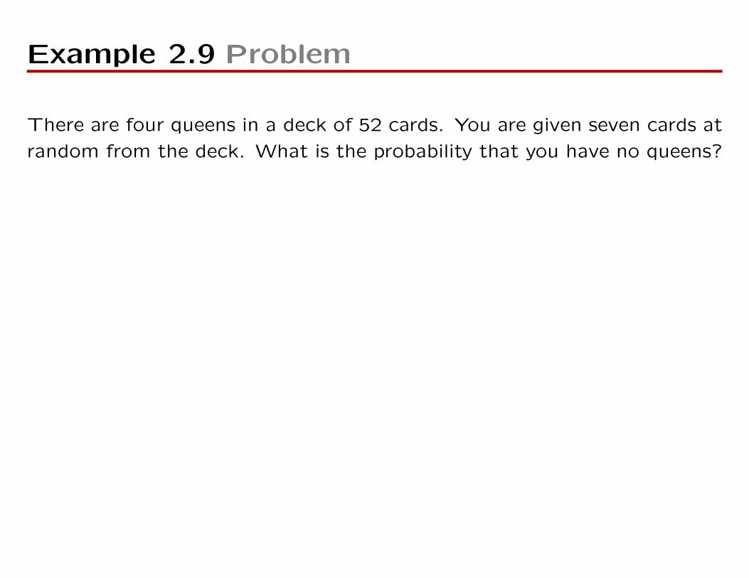
Example 2.9 Problem

There are four queens in a deck of 52 cards. You are given seven cards at

random from the deck. What is the probability that you have no queens?

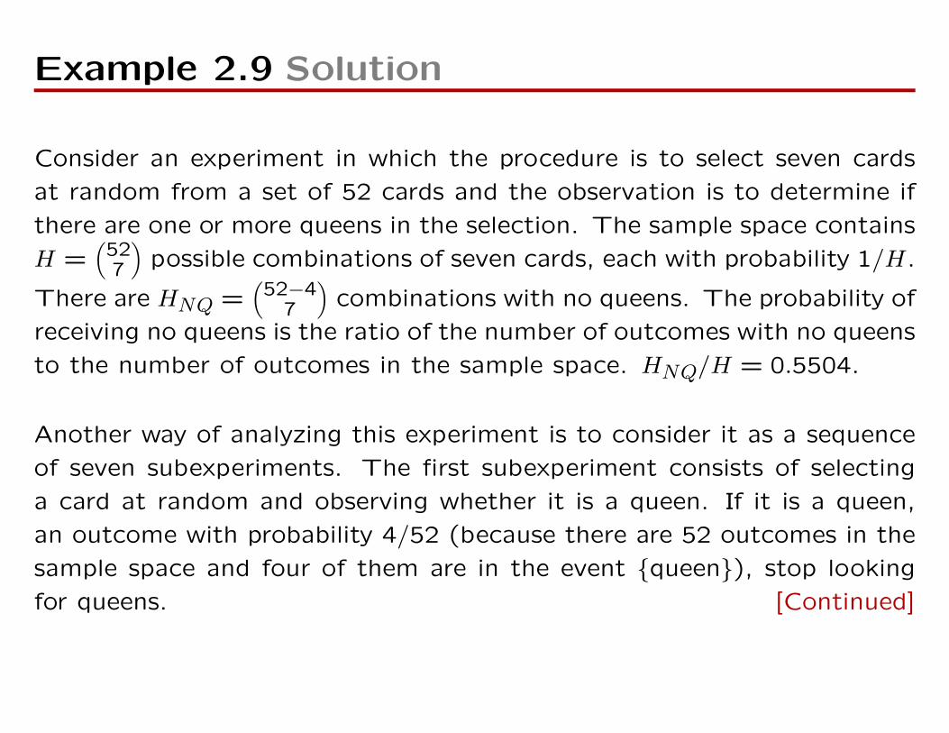
Example 2.9 Solution

Consider an experiment in which the procedure is to select seven cards

at random from a set of 52 cards and the observation is to determine if

there are one or more queens in the selection. The sample space contains

H =(

527

)possible combinations of seven cards, each with probability 1/H.

There are HNQ =(

52−47

)combinations with no queens. The probability of

receiving no queens is the ratio of the number of outcomes with no queens

to the number of outcomes in the sample space. HNQ/H = 0.5504.

Another way of analyzing this experiment is to consider it as a sequence

of seven subexperiments. The first subexperiment consists of selecting

a card at random and observing whether it is a queen. If it is a queen,

an outcome with probability 4/52 (because there are 52 outcomes in the

sample space and four of them are in the event queen), stop looking

for queens. [Continued]

Example 2.9 Solution (Continued 2)

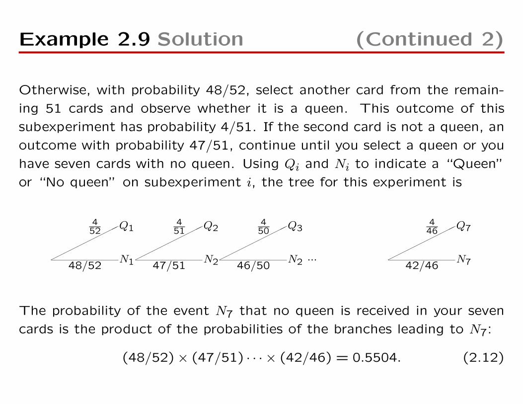
Otherwise, with probability 48/52, select another card from the remain-

ing 51 cards and observe whether it is a queen. This outcome of this

subexperiment has probability 4/51. If the second card is not a queen, an

outcome with probability 47/51, continue until you select a queen or you

have seven cards with no queen. Using Qi and Ni to indicate a “Queen”

or “No queen” on subexperiment i, the tree for this experiment is

Q1

452

N148/52

Q2

451

N247/51

Q3

450

N246/50...

Q7

446

N742/46

The probability of the event N7 that no queen is received in your seven

cards is the product of the probabilities of the branches leading to N7:

(48/52)× (47/51) · · · × (42/46) = 0.5504. (2.12)

Example 2.10 Problem

There are four queens in a deck of 52 cards. You are given seven cards

at random from the deck. After receiving each card you return it to the

deck and receive another card at random. Observe whether you have not

received any queens among the seven cards you were given. What is the

probability that you have received no queens?

Example 2.10 Solution

The sample space contains 527 outcomes. There are 487 outcomes with

no queens. The ratio is (48/52)7 = 0.5710, the probability of receiv-

ing no queens. If this experiment is considered as a sequence of seven

subexperiments, the tree looks the same as the tree in Example 2.9, ex-

cept that all the horizontal branches have probability 48/52 and all the

diagonal branches have probability 4/52.

Theorem 2.4

Given m distinguishable objects, there are mn ways to choose with re-

placement an ordered sample of n objects.

Example 2.11

There are 210 = 1024 binary sequences of length 10.

Example 2.12

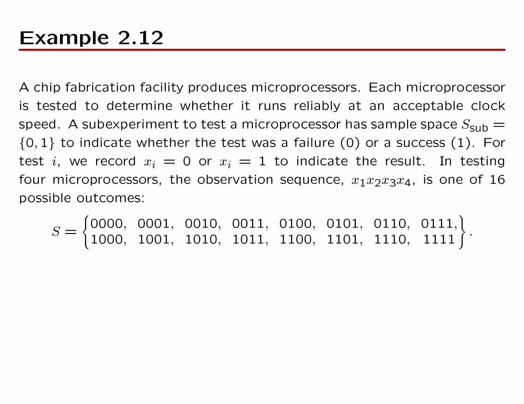
A chip fabrication facility produces microprocessors. Each microprocessor

is tested to determine whether it runs reliably at an acceptable clock

speed. A subexperiment to test a microprocessor has sample space Ssub =

0,1 to indicate whether the test was a failure (0) or a success (1). For

test i, we record xi = 0 or xi = 1 to indicate the result. In testing

four microprocessors, the observation sequence, x1x2x3x4, is one of 16

possible outcomes:

S =

0000, 0001, 0010, 0011, 0100, 0101, 0110, 0111,1000, 1001, 1010, 1011, 1100, 1101, 1110, 1111

.

Theorem 2.5

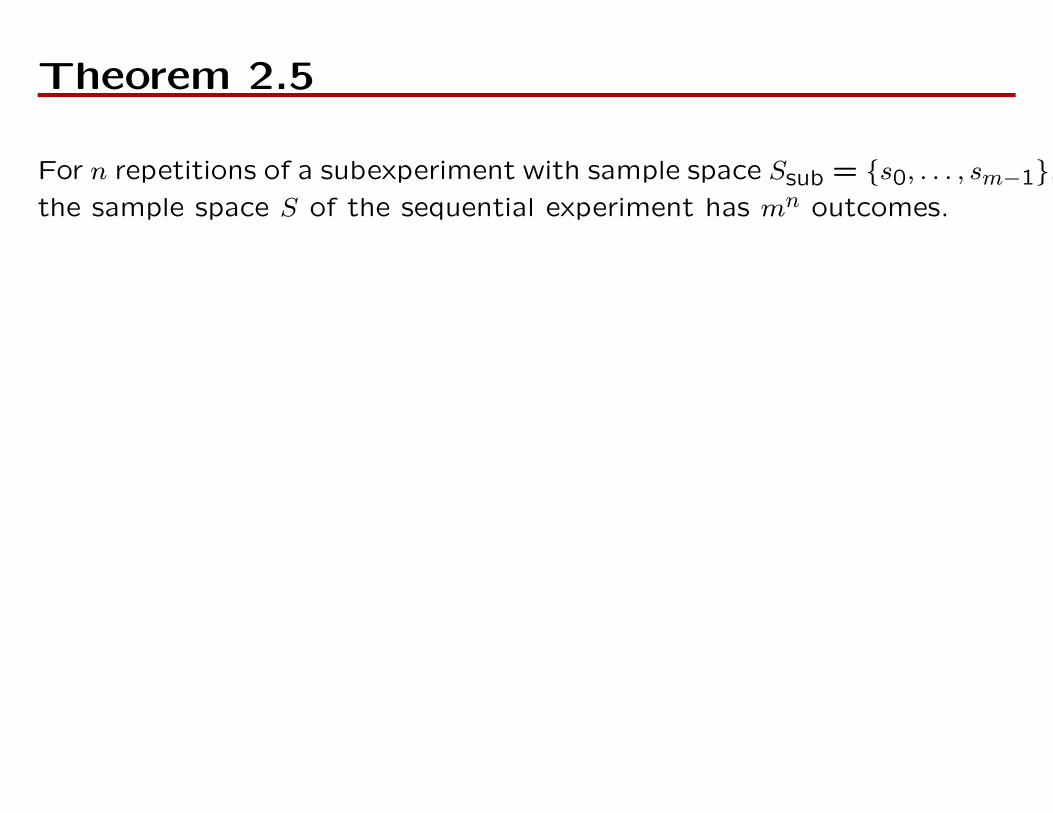
For n repetitions of a subexperiment with sample space Ssub = s0, . . . , sm−1,the sample space S of the sequential experiment has mn outcomes.

Example 2.13

There are ten students in a probability class; each earns a grade s ∈Ssub = A,B,C, F. We use the notation xi to denote the grade of the

ith student. For example, the grades for the class could be

x1x2 · · ·x10 = CBBACFBACF (2.13)

The sample space S of possible sequences contains 410 = 1,048,576

outcomes.

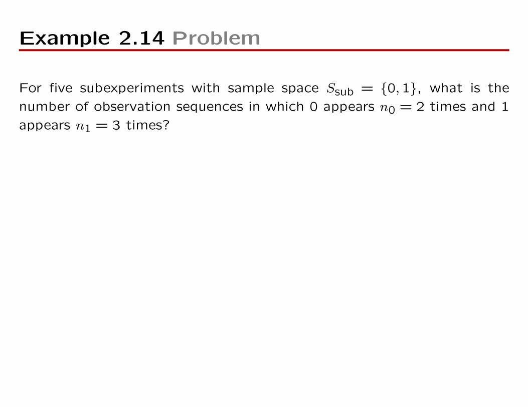
Example 2.14 Problem

For five subexperiments with sample space Ssub = 0,1, what is the

number of observation sequences in which 0 appears n0 = 2 times and 1

appears n1 = 3 times?

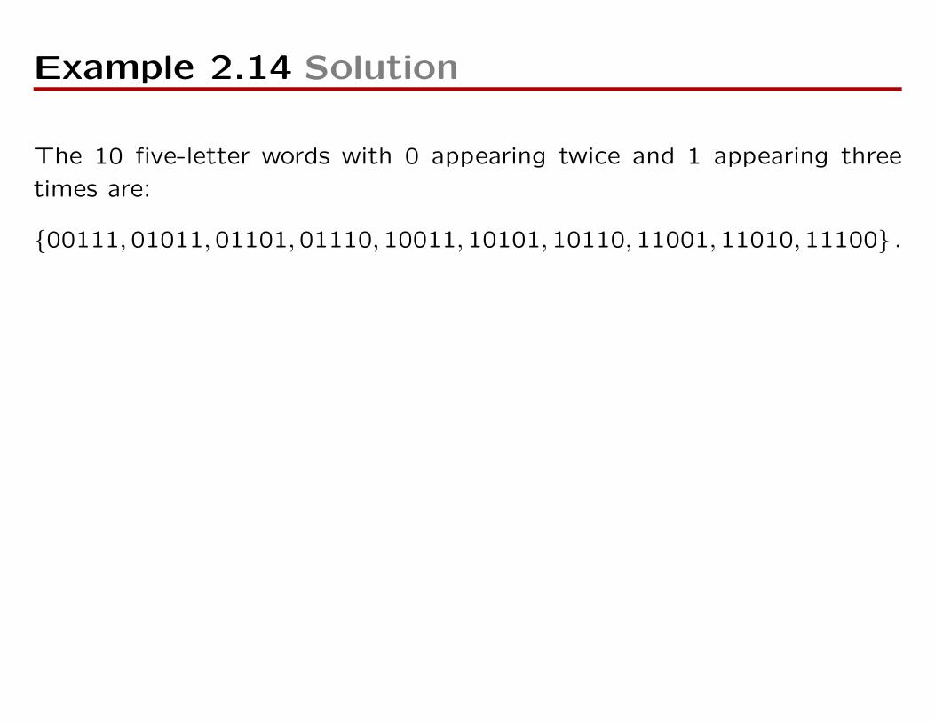
Example 2.14 Solution

The 10 five-letter words with 0 appearing twice and 1 appearing three

times are:

00111,01011,01101,01110,10011,10101,10110,11001,11010,11100 .

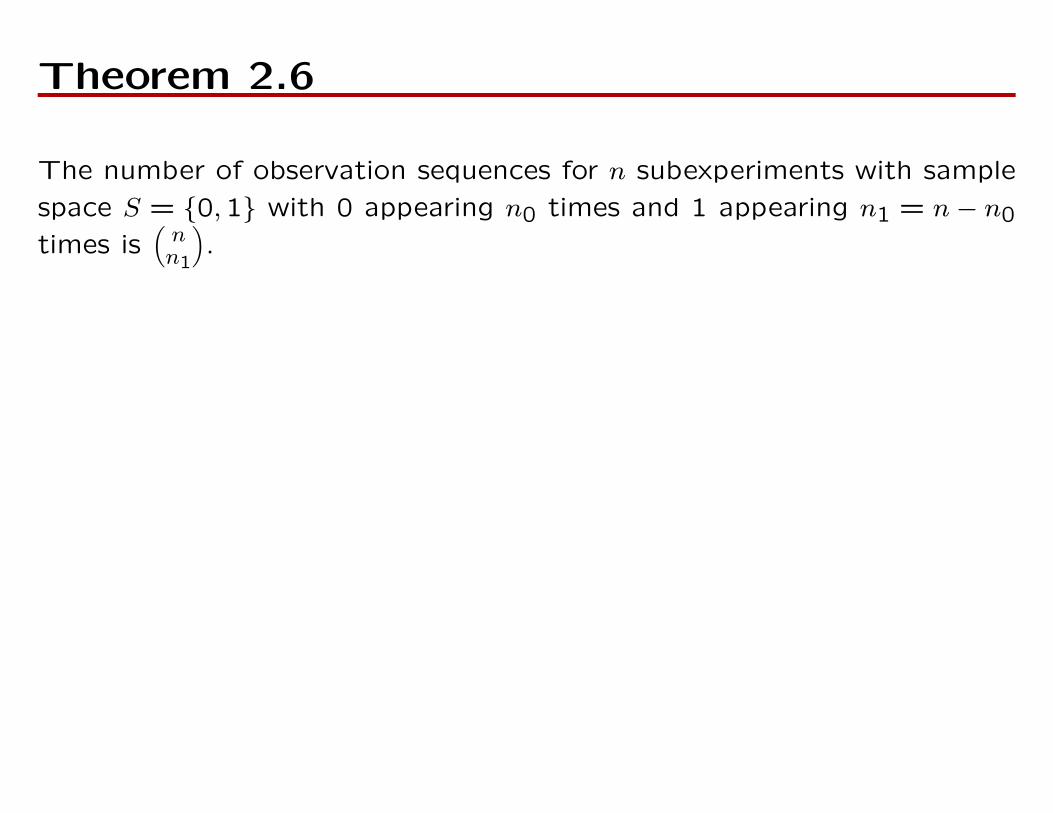
Theorem 2.6

The number of observation sequences for n subexperiments with sample

space S = 0,1 with 0 appearing n0 times and 1 appearing n1 = n− n0

times is(nn1

).

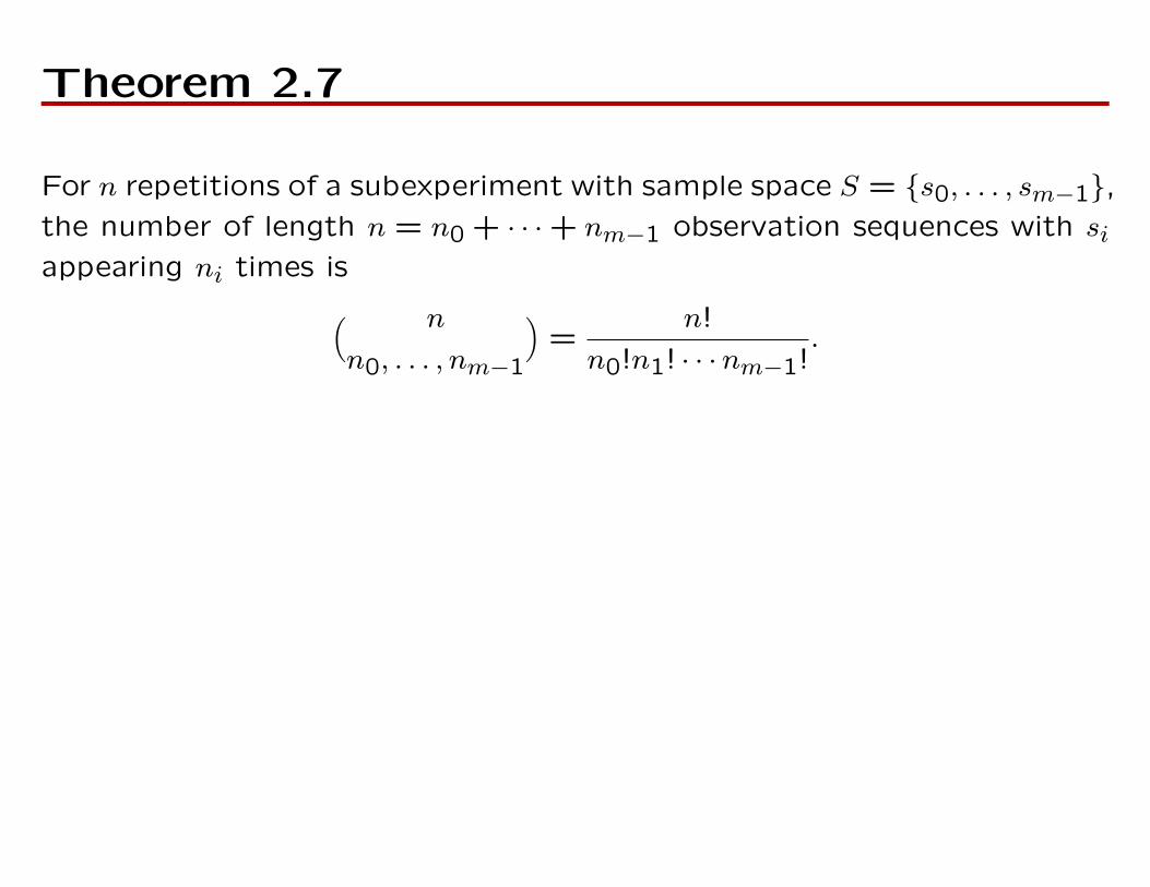
Theorem 2.7

For n repetitions of a subexperiment with sample space S = s0, . . . , sm−1,the number of length n = n0 + · · ·+ nm−1 observation sequences with siappearing ni times is( n

n0, . . . , nm−1

)=

n!

n0!n1! · · ·nm−1!.

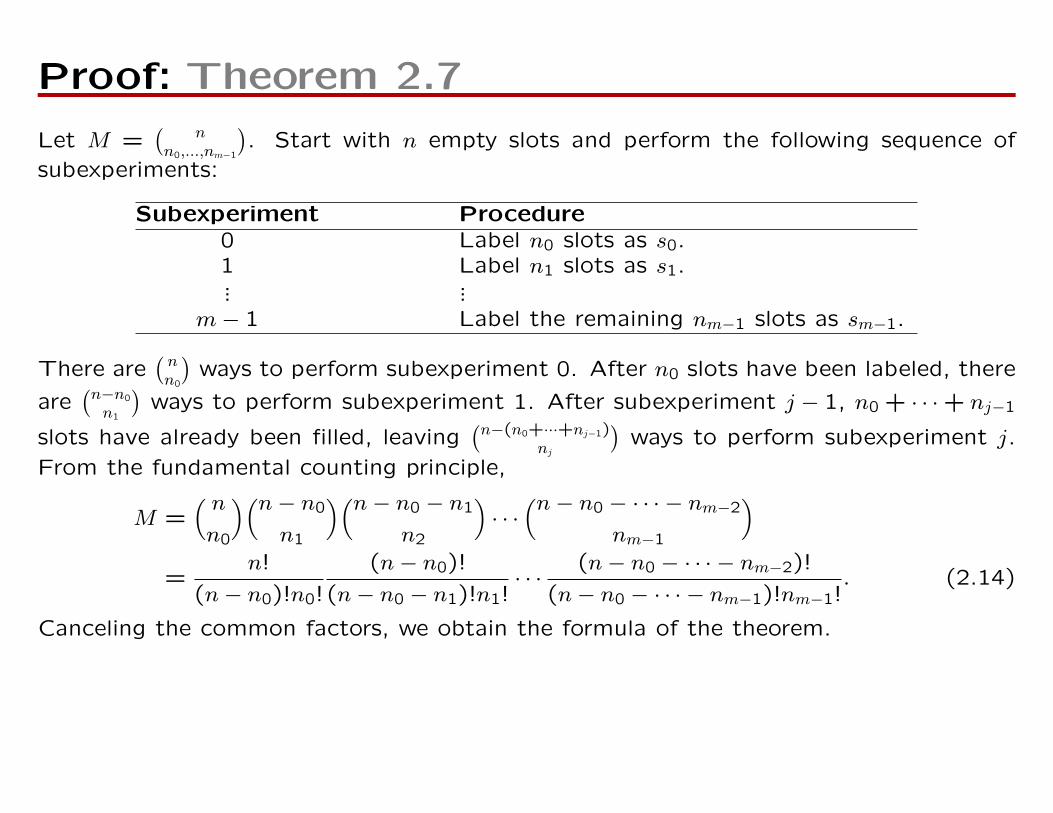
Proof: Theorem 2.7

Let M =(

nn0,...,nm−1

). Start with n empty slots and perform the following sequence of

subexperiments:

Subexperiment Procedure0 Label n0 slots as s0.1 Label n1 slots as s1.... ...

m− 1 Label the remaining nm−1 slots as sm−1.

There are(nn0

)ways to perform subexperiment 0. After n0 slots have been labeled, there

are(n−n0

n1

)ways to perform subexperiment 1. After subexperiment j − 1, n0 + · · ·+ nj−1

slots have already been filled, leaving(n−(n0+···+nj−1)

nj

)ways to perform subexperiment j.

From the fundamental counting principle,

M =( nn0

)(n− n0

n1

)(n− n0 − n1

n2

)· · ·(n− n0 − · · · − nm−2

nm−1

)=

n!

(n− n0)!n0!

(n− n0)!

(n− n0 − n1)!n1!· · ·

(n− n0 − · · · − nm−2)!

(n− n0 − · · · − nm−1)!nm−1!. (2.14)

Canceling the common factors, we obtain the formula of the theorem.

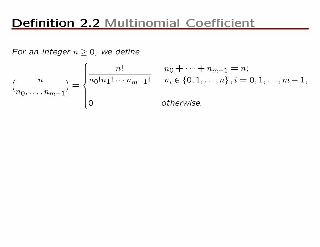
Definition 2.2 Multinomial Coefficient

For an integer n ≥ 0, we define

( n

n0, . . . , nm−1

)=

n!

n0!n1! · · ·nm−1!

n0 + · · ·+ nm−1 = n;

ni ∈ 0,1, . . . , n , i = 0,1, . . . ,m− 1,

0 otherwise.

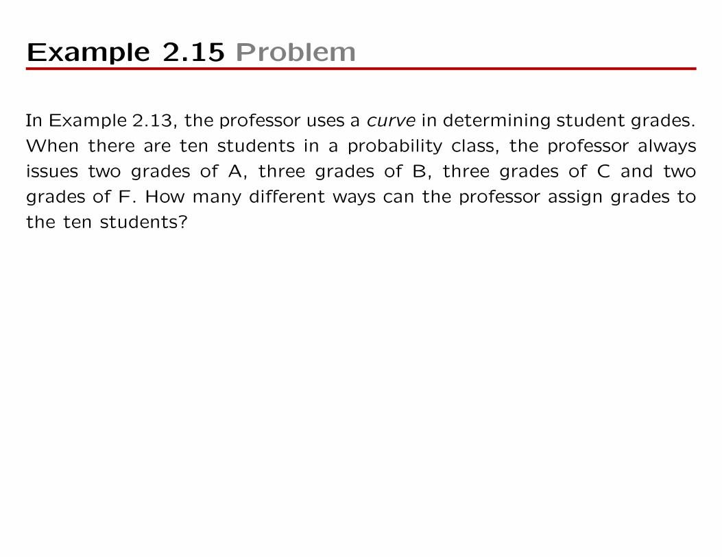
Example 2.15 Problem

In Example 2.13, the professor uses a curve in determining student grades.

When there are ten students in a probability class, the professor always

issues two grades of A, three grades of B, three grades of C and two

grades of F. How many different ways can the professor assign grades to

the ten students?

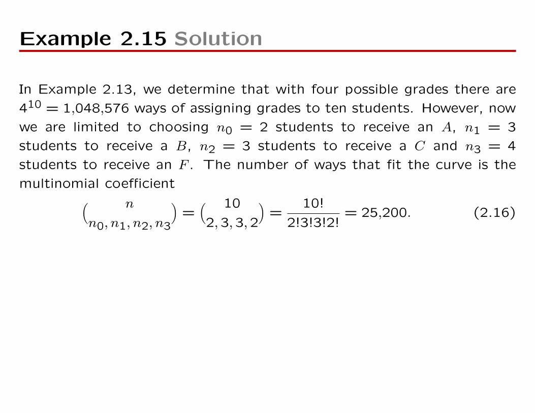
Example 2.15 Solution

In Example 2.13, we determine that with four possible grades there are

410 = 1,048,576 ways of assigning grades to ten students. However, now

we are limited to choosing n0 = 2 students to receive an A, n1 = 3

students to receive a B, n2 = 3 students to receive a C and n3 = 4

students to receive an F . The number of ways that fit the curve is the

multinomial coefficient( n

n0, n1, n2, n3

)=( 10

2,3,3,2

)=

10!

2!3!3!2!= 25,200. (2.16)

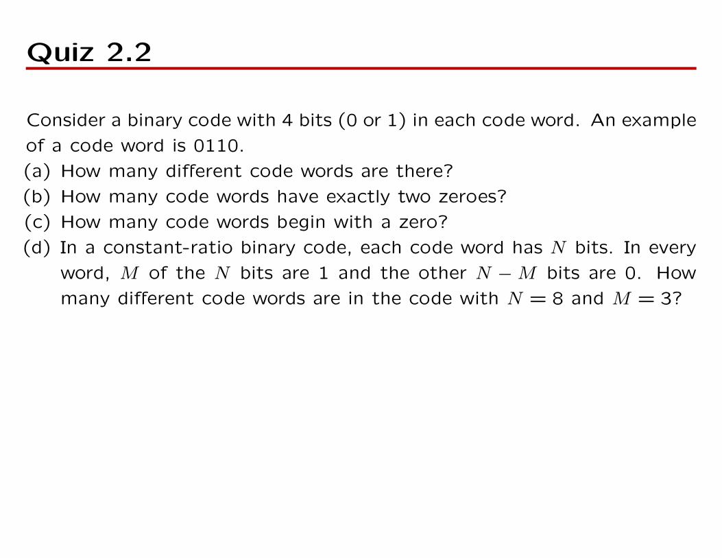
Quiz 2.2

Consider a binary code with 4 bits (0 or 1) in each code word. An example

of a code word is 0110.

(a) How many different code words are there?

(b) How many code words have exactly two zeroes?

(c) How many code words begin with a zero?

(d) In a constant-ratio binary code, each code word has N bits. In every

word, M of the N bits are 1 and the other N −M bits are 0. How

many different code words are in the code with N = 8 and M = 3?

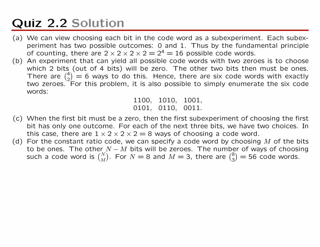
Quiz 2.2 Solution(a) We can view choosing each bit in the code word as a subexperiment. Each subex-

periment has two possible outcomes: 0 and 1. Thus by the fundamental principleof counting, there are 2× 2× 2× 2 = 24 = 16 possible code words.

(b) An experiment that can yield all possible code words with two zeroes is to choosewhich 2 bits (out of 4 bits) will be zero. The other two bits then must be ones.There are

(42

)= 6 ways to do this. Hence, there are six code words with exactly

two zeroes. For this problem, it is also possible to simply enumerate the six codewords:

1100, 1010, 1001,0101, 0110, 0011.

(c) When the first bit must be a zero, then the first subexperiment of choosing the firstbit has only one outcome. For each of the next three bits, we have two choices. Inthis case, there are 1× 2× 2× 2 = 8 ways of choosing a code word.

(d) For the constant ratio code, we can specify a code word by choosing M of the bitsto be ones. The other N −M bits will be zeroes. The number of ways of choosingsuch a code word is

(NM

). For N = 8 and M = 3, there are

(83

)= 56 code words.

Section 2.3

Independent Trials

Example 2.16 Problem

What is the probability P[E2,3] of two failures and three successes in five

independent trials with success probability p.

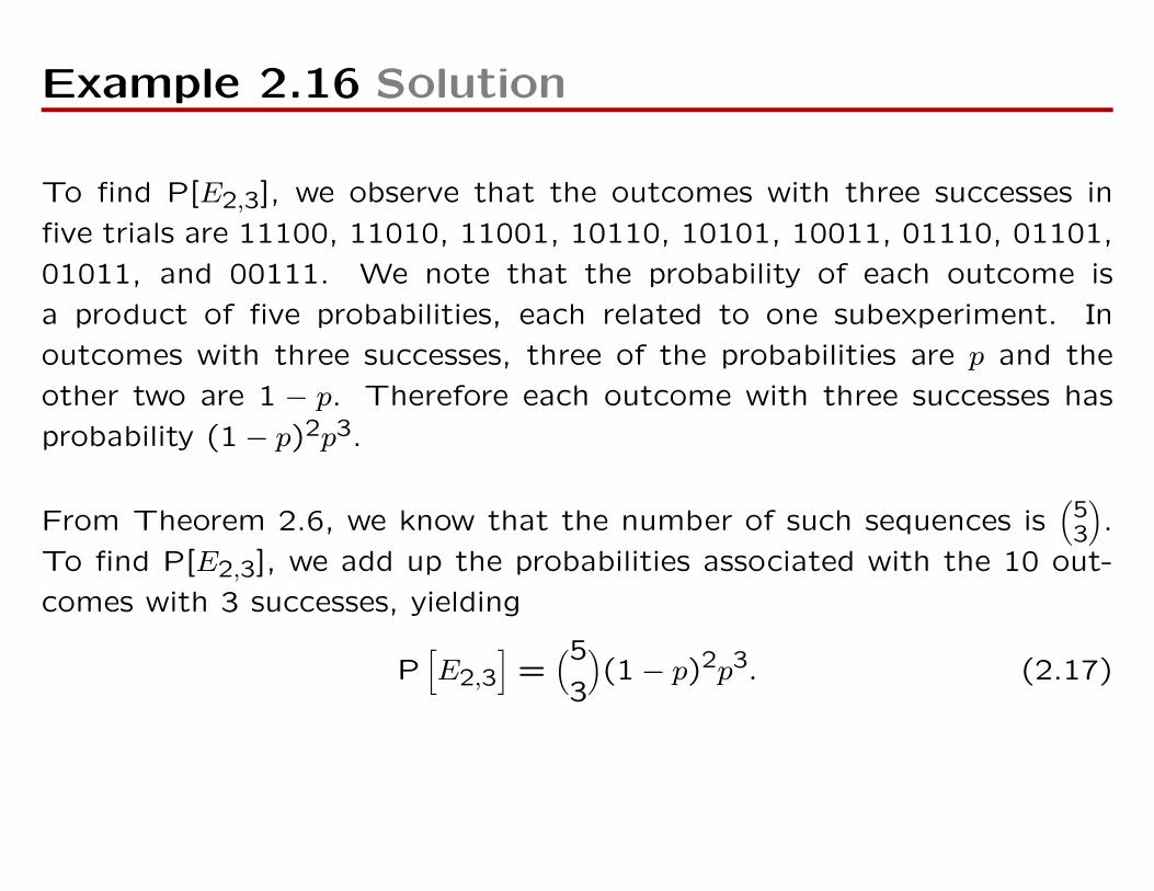
Example 2.16 Solution

To find P[E2,3], we observe that the outcomes with three successes in

five trials are 11100, 11010, 11001, 10110, 10101, 10011, 01110, 01101,

01011, and 00111. We note that the probability of each outcome is

a product of five probabilities, each related to one subexperiment. In

outcomes with three successes, three of the probabilities are p and the

other two are 1 − p. Therefore each outcome with three successes has

probability (1− p)2p3.

From Theorem 2.6, we know that the number of such sequences is(

53

).

To find P[E2,3], we add up the probabilities associated with the 10 out-

comes with 3 successes, yielding

P[E2,3

]=(53

)(1− p)2p3. (2.17)

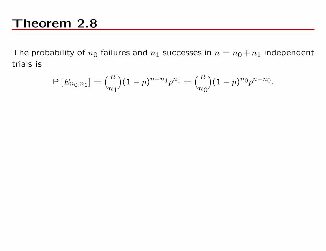
Theorem 2.8

The probability of n0 failures and n1 successes in n = n0+n1 independent

trials is

P[En0,n1

]=( nn1

)(1− p)n−n1pn1 =

( nn0

)(1− p)n0pn−n0.

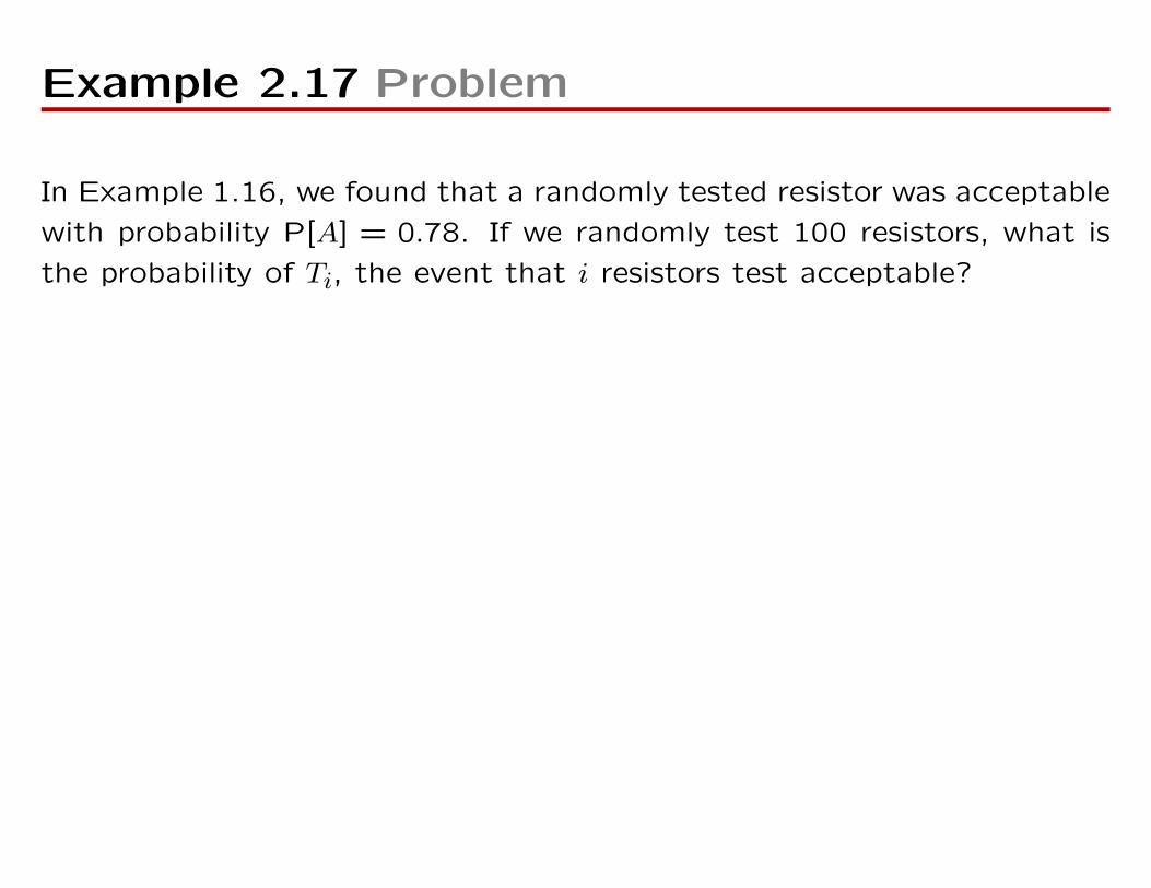
Example 2.17 Problem

In Example 1.16, we found that a randomly tested resistor was acceptable

with probability P[A] = 0.78. If we randomly test 100 resistors, what is

the probability of Ti, the event that i resistors test acceptable?

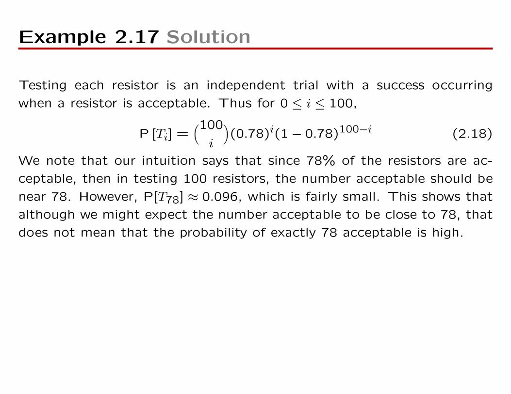
Example 2.17 Solution

Testing each resistor is an independent trial with a success occurring

when a resistor is acceptable. Thus for 0 ≤ i ≤ 100,

P [Ti] =(100

i

)(0.78)i(1− 0.78)100−i (2.18)

We note that our intuition says that since 78% of the resistors are ac-

ceptable, then in testing 100 resistors, the number acceptable should be

near 78. However, P[T78] ≈ 0.096, which is fairly small. This shows that

although we might expect the number acceptable to be close to 78, that

does not mean that the probability of exactly 78 acceptable is high.

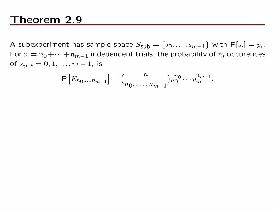
Theorem 2.9

A subexperiment has sample space Ssub = s0, . . . , sm−1 with P[si] = pi.

For n = n0+· · ·+nm−1 independent trials, the probability of ni occurences

of si, i = 0,1, . . . ,m− 1, is

P[En0,...,nm−1

]=( n

n0, . . . , nm−1

)pn00 · · · p

nm−1m−1 .

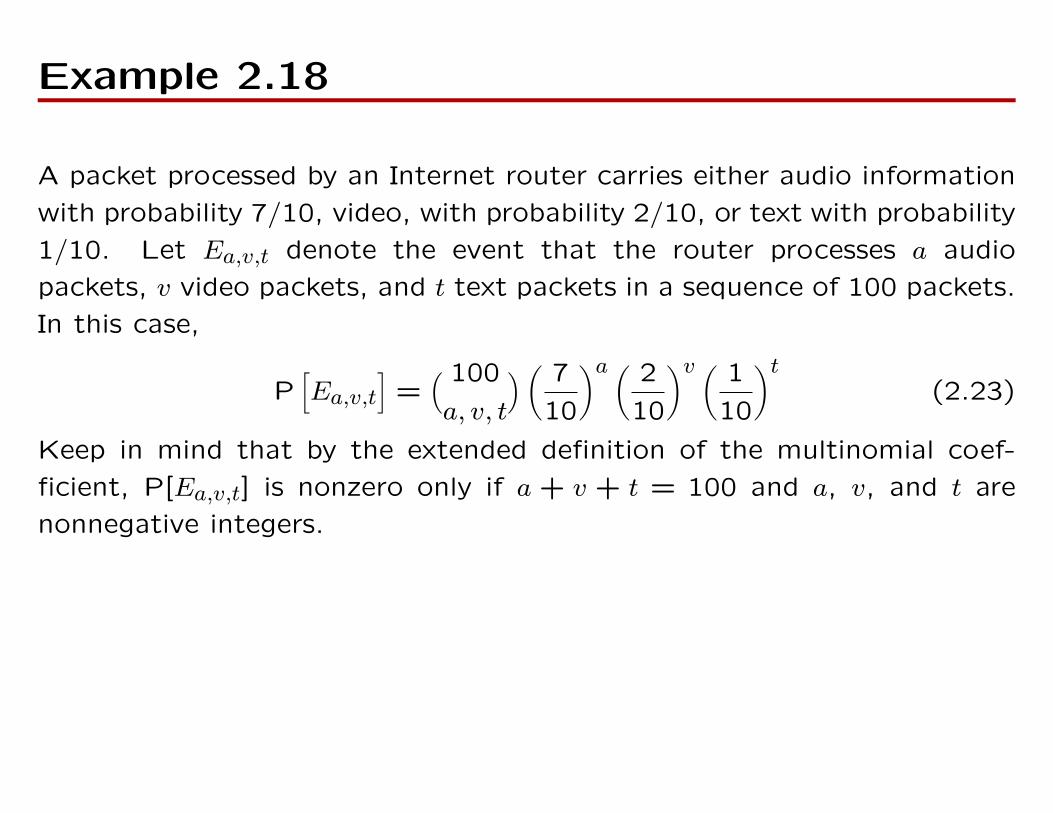
Example 2.18

A packet processed by an Internet router carries either audio information

with probability 7/10, video, with probability 2/10, or text with probability

1/10. Let Ea,v,t denote the event that the router processes a audio

packets, v video packets, and t text packets in a sequence of 100 packets.

In this case,

P[Ea,v,t

]=( 100

a, v, t

) ( 7

10

)a ( 2

10

)v ( 1

10

)t(2.23)

Keep in mind that by the extended definition of the multinomial coef-

ficient, P[Ea,v,t] is nonzero only if a + v + t = 100 and a, v, and t are

nonnegative integers.

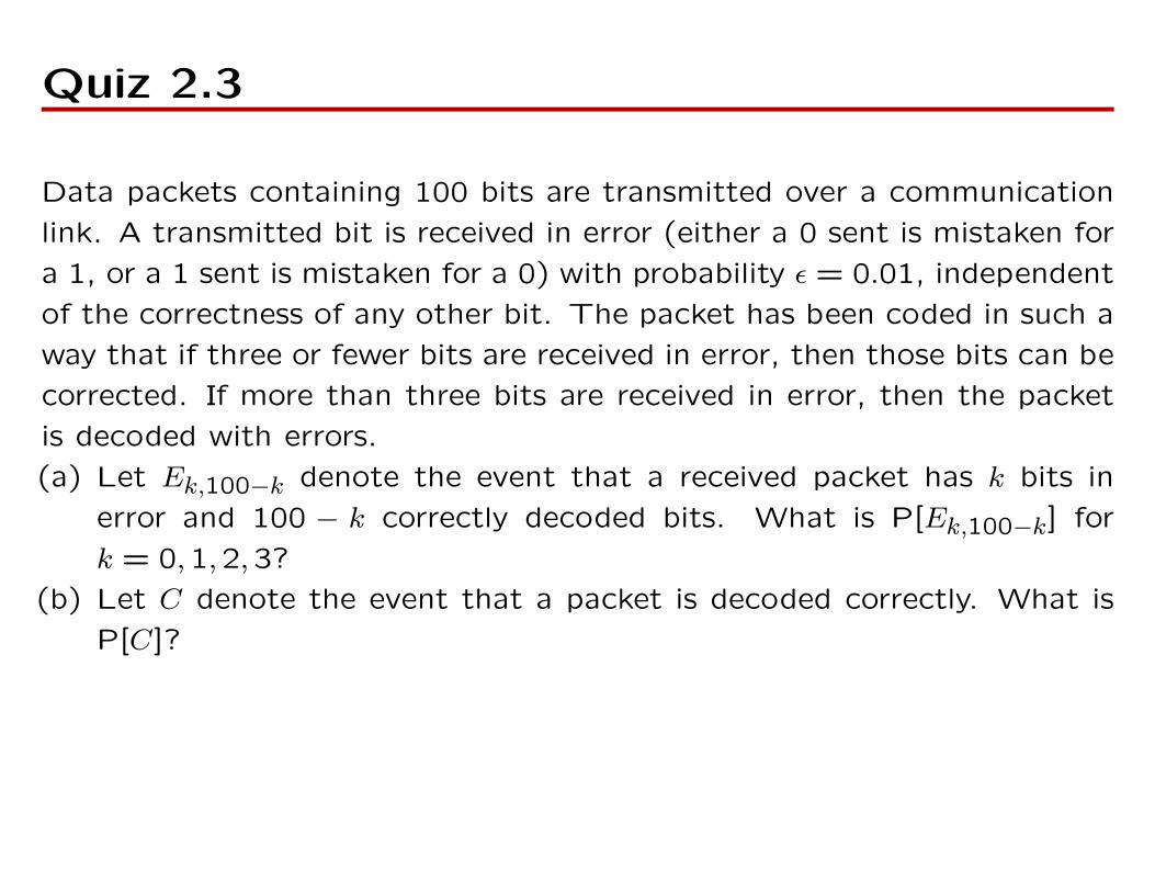
Quiz 2.3

Data packets containing 100 bits are transmitted over a communication

link. A transmitted bit is received in error (either a 0 sent is mistaken for

a 1, or a 1 sent is mistaken for a 0) with probability ε = 0.01, independent

of the correctness of any other bit. The packet has been coded in such a

way that if three or fewer bits are received in error, then those bits can be

corrected. If more than three bits are received in error, then the packet

is decoded with errors.

(a) Let Ek,100−k denote the event that a received packet has k bits in

error and 100 − k correctly decoded bits. What is P[Ek,100−k] for

k = 0,1,2,3?

(b) Let C denote the event that a packet is decoded correctly. What is

P[C]?

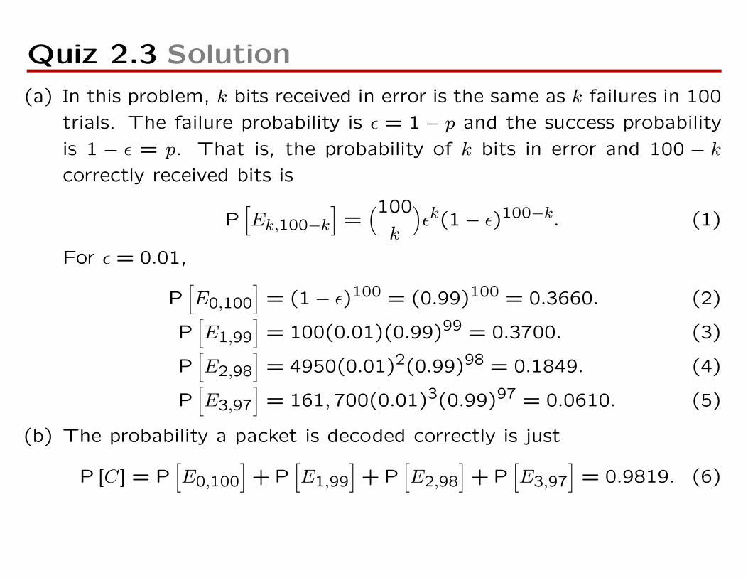
Quiz 2.3 Solution

(a) In this problem, k bits received in error is the same as k failures in 100

trials. The failure probability is ε = 1− p and the success probability

is 1 − ε = p. That is, the probability of k bits in error and 100 − kcorrectly received bits is

P[Ek,100−k

]=(100

k

)εk(1− ε)100−k. (1)

For ε = 0.01,

P[E0,100

]= (1− ε)100 = (0.99)100 = 0.3660. (2)

P[E1,99

]= 100(0.01)(0.99)99 = 0.3700. (3)

P[E2,98

]= 4950(0.01)2(0.99)98 = 0.1849. (4)

P[E3,97

]= 161,700(0.01)3(0.99)97 = 0.0610. (5)

(b) The probability a packet is decoded correctly is just

P [C] = P[E0,100

]+ P

[E1,99

]+ P

[E2,98

]+ P

[E3,97

]= 0.9819. (6)

Section 2.4

Matlab

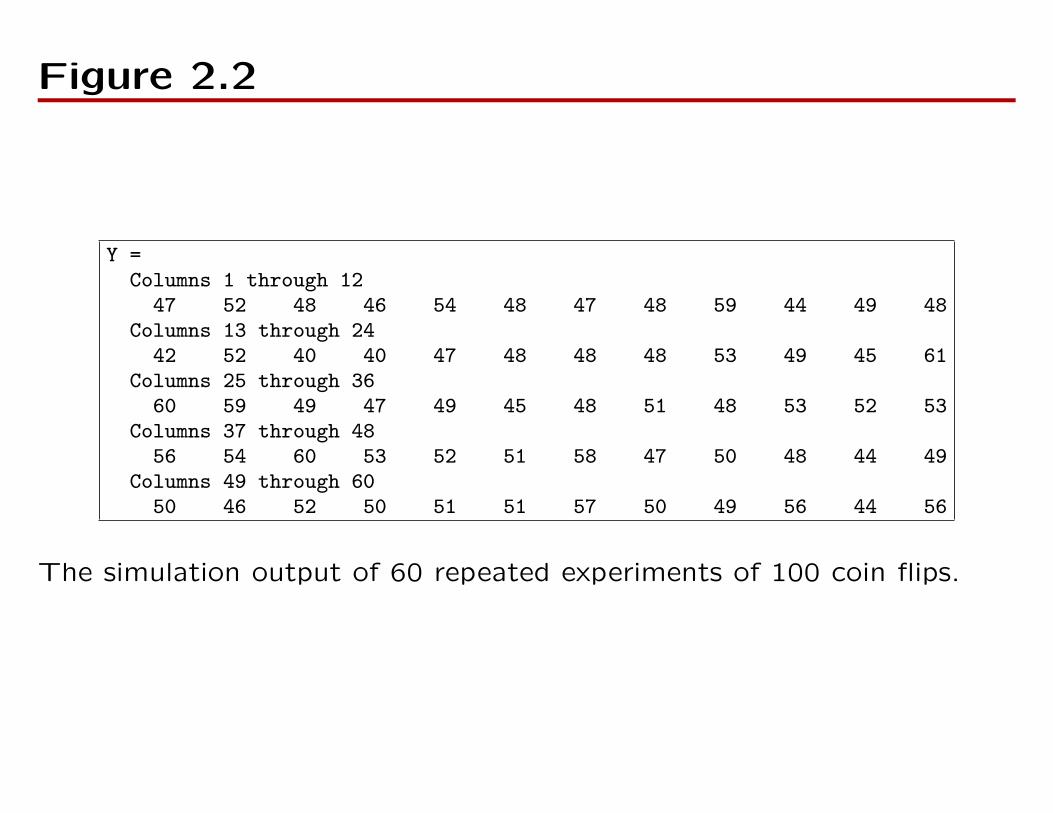
Figure 2.2

Y =Columns 1 through 12

47 52 48 46 54 48 47 48 59 44 49 48Columns 13 through 24

42 52 40 40 47 48 48 48 53 49 45 61Columns 25 through 36

60 59 49 47 49 45 48 51 48 53 52 53Columns 37 through 48

56 54 60 53 52 51 58 47 50 48 44 49Columns 49 through 60

50 46 52 50 51 51 57 50 49 56 44 56

The simulation output of 60 repeated experiments of 100 coin flips.

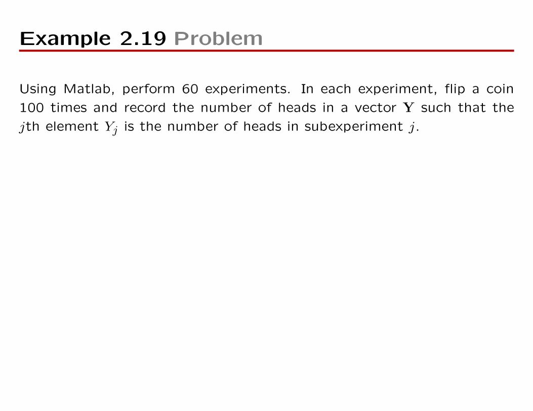
Example 2.19 Problem

Using Matlab, perform 60 experiments. In each experiment, flip a coin

100 times and record the number of heads in a vector Y such that the

jth element Yj is the number of heads in subexperiment j.

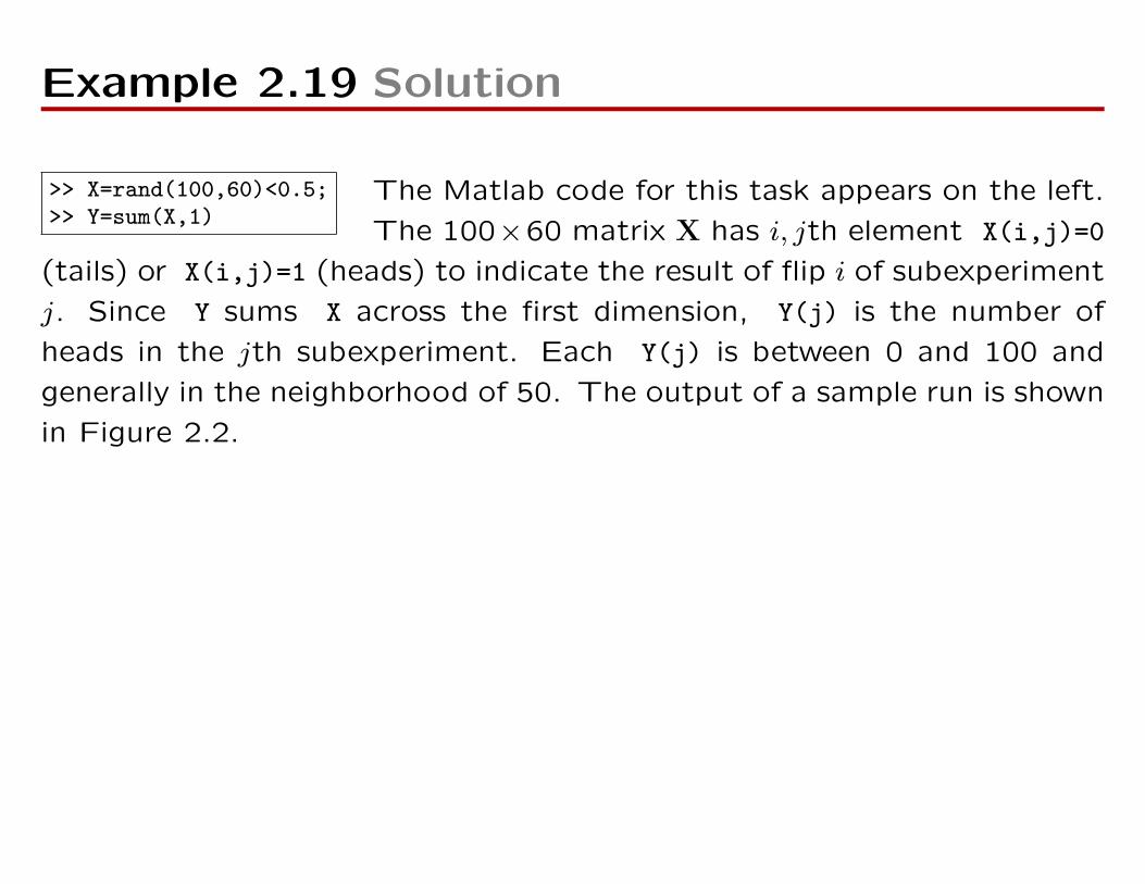
Example 2.19 Solution

>> X=rand(100,60)<0.5;>> Y=sum(X,1)

The Matlab code for this task appears on the left.

The 100×60 matrix X has i, jth element X(i,j)=0

(tails) or X(i,j)=1 (heads) to indicate the result of flip i of subexperiment

j. Since Y sums X across the first dimension, Y(j) is the number of

heads in the jth subexperiment. Each Y(j) is between 0 and 100 and

generally in the neighborhood of 50. The output of a sample run is shown

in Figure 2.2.

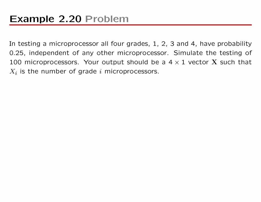
Example 2.20 Problem

In testing a microprocessor all four grades, 1, 2, 3 and 4, have probability

0.25, independent of any other microprocessor. Simulate the testing of

100 microprocessors. Your output should be a 4× 1 vector X such that

Xi is the number of grade i microprocessors.

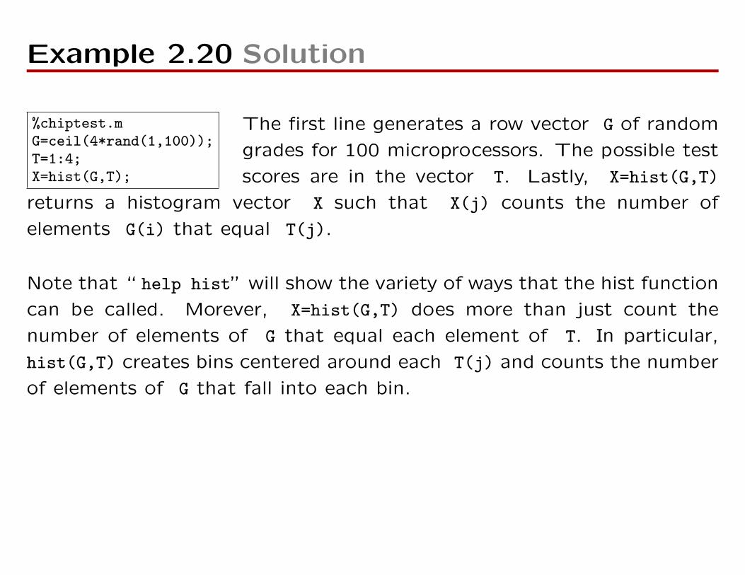
Example 2.20 Solution

%chiptest.mG=ceil(4*rand(1,100));T=1:4;X=hist(G,T);

The first line generates a row vector G of random

grades for 100 microprocessors. The possible test

scores are in the vector T. Lastly, X=hist(G,T)

returns a histogram vector X such that X(j) counts the number of

elements G(i) that equal T(j).

Note that “ help hist” will show the variety of ways that the hist function

can be called. Morever, X=hist(G,T) does more than just count the

number of elements of G that equal each element of T. In particular,

hist(G,T) creates bins centered around each T(j) and counts the number

of elements of G that fall into each bin.

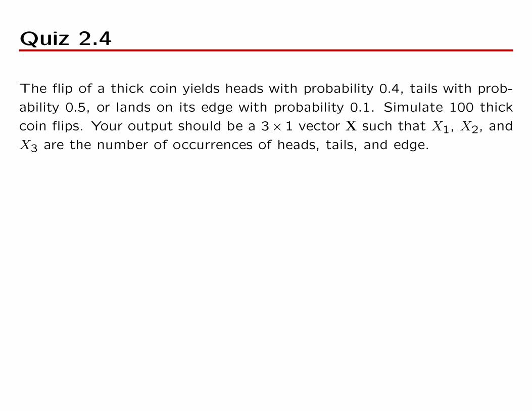
Quiz 2.4

The flip of a thick coin yields heads with probability 0.4, tails with prob-

ability 0.5, or lands on its edge with probability 0.1. Simulate 100 thick

coin flips. Your output should be a 3×1 vector X such that X1, X2, and

X3 are the number of occurrences of heads, tails, and edge.

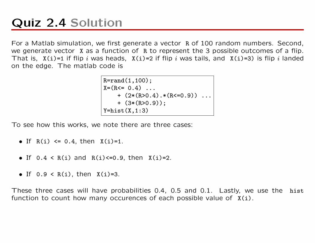
Quiz 2.4 Solution

For a Matlab simulation, we first generate a vector R of 100 random numbers. Second,we generate vector X as a function of R to represent the 3 possible outcomes of a flip.That is, X(i)=1 if flip i was heads, X(i)=2 if flip i was tails, and X(i)=3) is flip i landedon the edge. The matlab code is

R=rand(1,100);X=(R<= 0.4) ...

+ (2*(R>0.4).*(R<=0.9)) ...+ (3*(R>0.9));

Y=hist(X,1:3)

To see how this works, we note there are three cases:

• If R(i) <= 0.4, then X(i)=1.

• If 0.4 < R(i) and R(i)<=0.9, then X(i)=2.

• If 0.9 < R(i), then X(i)=3.

These three cases will have probabilities 0.4, 0.5 and 0.1. Lastly, we use the histfunction to count how many occurences of each possible value of X(i).