Treatment Misallocation

(Preliminary, Comments Welcome)

Debopam Bhattacharya,

University of Oxford

First draft February, 2009.This draft: July, 2010.

Abstract

In real-life, individuals are often assigned to binary treatments based on es-

tablished covariate-based protocols. Direct or implicit taste-based discrimination

would make such protocols economically ine¢ cient in that the expected gain from

treatment would be smaller for a subset of the currently treated than the currently

untreated. We present a framework for detecting such ine¢ ciency using a partial

identi�cation approach which continues to work when the decision-maker observes

more covariates than us. We also propose a novel way of inferring the relevant

counterfactual distributions by combining observational datasets with experimen-

tal estimates. The method can be extended to (partially) infer risk-preferences of

the decision-maker, under which observed allocations are e¢ cient. The most risk

neutral solution may be obtained via maximizing entropy. We outline the theory of

inference and study the e¢ cacy of our methodology using a simulation exercise. Our

methods apply when individuals cannot alter their potential treatment outcomes in

response to the decision-maker�s actions unlike the case of law enforcement (c.f.,

Knowles, Persico and Todd (2001)).

1 Introduction

In many real-life situations, external decision-makers assign individuals to treatments.

Examples include banks approving mortgage and business loans, doctors referring patients

1

to surgery and �rms hiring interns. However, existing protocols for deciding treatment

status may be economically ine¢ cient in that the expected gain from treating a subgroup

of those currently being treated is smaller than that from treating a subset of the untreated

individuals, the expectation being taken with respect to the true underlying distribution

of the random variables concerned. This situation implies that the treatment, to be

thought of as a scarce resource, is being assigned among individuals in a way that does not

maximize its overall productivity. A leading cause of such ine¢ ciency is prejudice against

speci�c demographic groups� either direct or implicit� but ine¢ ciency can also arise

from the failure to condition on relevant covariates or systematic biases in the decision-

maker�s (DM, henceforth) subjective expectation. We present a framework for detecting

and analyzing such misallocation using a partial identi�cation approach. Unless one has

access to exactly the same variables as the DM, one can at best detect misallocation but

cannot in general infer if misallocation has occurred because of prejudice or some other,

perhaps more innocuous, reason.1

The present paper focuses on the case where the treatment in question is binary and

the outcome of interest either binary or continuous. We assume that an experienced DM

observes for each individual a set of covariates and assigns him/her to treatment based

on the expected gains from treatment, conditional on these covariate values. In this set-

up, a necessary condition for the DM�s assignment to be productively e¢ cient is that in

every observable covariate group, the expected net bene�t of treatment (relative to cost)

to the marginal treatment recipient, i.e., the "last person" to have received treatment

is weakly greater than a common threshold which, in turn, is greater than or equal to

the expected net bene�t of the "�rst person" to have been denied treatment. Here,

last and �rst refer to the types of individuals with the smallest and the largest expected

bene�t from treatment, respectively, where types are de�ned in terms of the characteristics

observed by the DM. Misallocation occurs when the bene�t to the marginal recipient

di¤ers signi�cantly across covariates and it can arise if, for instance, di¤erent thresholds

are used for di¤erent covariate groups, which would happen if the DM was prejudiced

against certain groups. The DM�s assignment results in an observational dataset, where

for each individual, we observe her treatment status, her outcome conditional on her

treatment status and a set of covariate values. The problem is to detect misallocation of

1Thus, here we are making a conscious distinction between "non-statistical discrimination" and

"prejudice"�a point on which we elaborate below.

2

treatment from this dataset.

Detecting ine¢ cient treatment allocation from such an observational dataset alone is

complicated by two reasons. The �rst is that the DM can base treatment assignment on

characteristics that are not observed by us. This makes it is hard, if not impossible, to

know who are the "marginal" treatment recipient and non-recipients�a problem already

recognized in the literature (c.f., Heckman (1998), Persico (2009)) and labeled "inframar-

ginality". Further, bene�ts are also hard to measure with a single observational dataset

because, as is well known, counterfactual means are not observed.

In this paper, we discuss a new approach to detecting misallocation in such situations.

The key idea is to use the notion of partial identi�cation, motivated by the implication of

e¢ cient allocation that expected net bene�ts in every subset of the treated group must

weakly exceed expected net bene�ts in every subset of the untreated group�a (condi-

tional) moment inequality condition. These moment inequalities for subsets de�ned by

covariates that the DM observes have testable implications for the (cruder) subsets based

on the covariates that we observe. These implications can therefore be tested. Secondly,

we propose a novel way to identify the necessary counterfactual means by combining an

observational dataset with experimental estimates on subjects drawn from the same pop-

ulation. The latter supplements existing methods of identifying counterfactuals using,

say, instrumental variables.

The bulk of our analysis rests upon three assumptions. The �rst is that the DM

is experienced in the sense that he can form correct expectations. The second is that

the DM observes and can condition treatment allocation on all the characteristics (and

possibly more than) those that we observe. Third, we observe the same outcomes whose

expectations, taken by the DM, should logically determine treatment assignment in the

observational dataset.

The third assumption simply clari�es that the de�nition of productivity (with respect

to which ine¢ ciency is de�ned) must be unanimously agreed upon and this common

measure of productivity should be observable and veri�able. The second assumption seems

quite natural; but we discuss below in section 4 when it might fail and the implications

thereof. The �rst assumption�a "rational expectations" idea� is part of our de�nition

of e¢ ciency, i.e., we are testing the joint hypothesis that the DM can calculate correct

expectations and is allocating treatment e¢ ciently, based on those calculations. In other

words, we do not distinguish between the cases where the DM�s subjective expectations

3

deviate from the true expectations in a speci�c, systematic way and lead to the ine¢ ciency

observed and the case where the DM can form correct expectations but ends up with an

ine¢ cient allocation due to, say, prejudice against speci�c demographic groups. Indeed,

from a purely economic point of view, the implication for productivity loss in these two

cases is identical.2

The rest of the paper is organized as follows. Section 2 discusses the contribution of

the present paper in relation to the existing literature in economics and econometrics.

Section 3 presents the partial identi�cation methodology, discusses how counterfactuals

may be identi�ed via data combination and demonstrates how the analysis is robust to

failure of a key identical distribution assumption which underlies the data combination

method. Section 4 discusses some, albeit subtle, di¢ culties which prevent one from pin-

pointing the cause of misallocation even when it has been detected. Section 5 discusses

the complementary problem of inferring a DM�s underlying risk-preferences which would

justify the current allocations as e¢ cient. Section 6 brie�y outlines the theory of inference.

Section 7 presents a simulation study and section 8 concludes.

We would like to end this section by re-emphasizing that our methodology can detect

ine¢ ciency of treatment assignment and identify the demographic group(s) that are suf-

fering as a result of it but it cannot distinguish between the various causes which might

lead a DM to such an allocation. The existing literature in economics sometimes uses the

term "statistical discrimination" to mean an e¢ cient allocation that leads to disparities

in treatment rates but, in our reading, it is unclear about whether "non-statistical" dis-

crimination can arise only from prejudice. The present paper analyzes this latter point

in somewhat greater details than previously attempted and presents some examples to

illustrate the subtleties involved in the analysis.

2 Literature and contributions

It is useful at this stage to contrast our work on detecting misallocation with some ex-

isting empirical approaches to detect "discrimination" in treating individuals. Recall the

key identi�cation problem, viz., that it is impossible to tell if the group receiving less

treatment does so because it is less endowed with those determinants of productivity

2Whether our analysis can form the legal basis for prosecuting an errant DM is a separate question

and outside the scope of the present analysis.

4

which we do not observe but the DM does or because the DM is prejudiced against that

group. Consequently, to distinguish between statistical and non-statistical sources of ob-

served treatment disparities, it is necessary to observe the �nal outcomes resulting from

alternative treatments. Final outcomes are hard to observe in some contexts, e.g., labour

productivity of hired individuals, but not so hard in some others, e.g., survival after med-

ical treatment or posession of illicit drugs revealed via police searches. Some existing

papers deal with the former situation (c.f., Betrand and Mullainathan (2005), Goldin and

Rouse (2007)) and base their analysis on the idea that there is an observable characteristic

(quality of CV�s in the case of BM and audition performance in the case of GR) which

is a su¢ cient determinant of the relevant productivity. Race or gender, in these papers,

are assumed to have no additional e¤ect on expected productivity. In contrast, a series

of studies (c.f., Knowles, Persico, Todd (2001) and the papers cited there) have examined

the problem of detecting taste-based prejudice separately from statistical discrimination

in the context of vehicle search by the police, using data on �nal outcomes (hit rates). The

key insight is that in law-enforcement contexts, potential treatment recipients can alter

their behaviour�and thus their potential outcome upon being treated�in response to the

treator�s behaviour. This argument enables them to solve the problem of "inframarginal-

ity" and test for the economic e¢ ciency of the existing allocation. While their approach

applies to many situations of interest, especially ones involving law enforcement, it is not

applicable to all situations of treatment assignment where misallocation is a concern. For

example, it is very di¢ cult�if not impossible�for patients to alter their potential health

outcomes with and without surgery in response to the nature of treatment protocols used

by doctors.

In independent and ongoing work, Chandra and Staiger (2010) consider the problem

of identifying provider prejudice in intensive treatments for heart- attacks. They use an

instrumental variable approach to identify counterfactuals and attempt to test equality

of treatment thresholds under a strong high-level assumption on the distribution of unob-

servables for the two groups being compared (e.g., males and females). Essentially, their

method works if either the c.d.f. of bene�t distribution of one group is simply that of the

other group, translated by a �xed amount, or if the unobservable distribution is identical

for the two groups, conditional on the observables�leading to a "single index" structure

(c.f., Powell (1994)). But the latter essentially assumes away the inframarginality problem

which is the central source of di¢ culty in detecting ine¢ ciency.

5

On the econometric side, our paper links the discrimination literature in economics

with the partial identi�cation approach, pioneered by Manski, that has been receiving

a lot of recent attention. Our paper attempts to show how one can use the partial

identi�cation idea to make progress in solving an important and di¢ cult detection problem

long recognized in the economics literature. In particular, we analyze the problem of

inferring the set of (sub)-utility functions of the DM which would rationalize an observed

allocation pattern. We also show that a maximum entropy solution in this case gives

us that admissible utility which is closest to risk neutrality and this solution is easy to

compute and report rather than the entire identi�ed set. This focus on �nding speci�c

parameter values which have intuitive or economic interpretation among all the ones

in an identi�ed set appears to be novel. It also raises interesting inferential problems

pertaining to optimization with stochastic constraints which, to our knowledge, have not

been explored before.

A series of papers in the forecasting literature propose testing rationality of forecasts

made by central agencies (c.f. Elliott, Komunjer and Timmerman (2005), Patton and

Timmerman (2007) etc.). The idea is to (point) estimate parameters of the loss-function

which rationalize the observed forecasts. The set-up in that literature assumes that the

action (i.e., the forecast) has no e¤ect on the distribution of the future outcome. In

contrast, the key issue in our set-up is that the action (treatment status) fundamentally

a¤ects the distribution of the outcome and so the methodology of forecast rationality tests

cannot be used in our problem.

Lastly, our identi�cation approach uses counterfactual means and we propose a novel

way of obtaining them by combining the observational dataset with estimates from an

experimental study where individuals were randomized in to and out of treatment. This

method works best when the experimental group is drawn from the same population as

the observational one. However, the method works even in the case where the individuals

willing to be randomized are worse (i.e., have worse outcomes with and without the

treatment) along unobserved dimensions, which is sometimes the case in medical trials.

The cost of this complication is that it will be harder for us to detect misallocation relative

to the case where the two distributions are identical.

6

3 Methodology

Denote outcome with and without treatment by Y0 and Y1, respectively and let �Y =

Y1� Y0. Analogously, de�ne C1 and C0 as the potential costs corresponding to treatmentand no treatment, respectively. Let W = (X;Z) denote the covariates observed by the

DM, where the component Z is not observed by us. Let X j denote the support of X for

the subpopulation who would be assigned D = j, j = 0; 1 by the DM and Esub denote

expectations taken w.r.t. the DM�s subjective probability distributions, P sub.

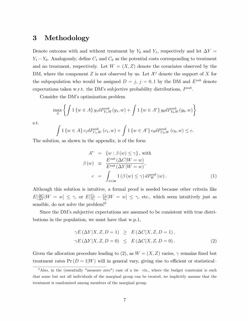
Consider the DM�s optimization problem

maxA

�Z1 fw 2 Ag y1dP subY1;W

(y1; w) +

Z1 fw 2 Acg y0dP subY0;W

(y0; w)

�s.t. Z

1 fw 2 Ag c1dP subC1;W(c1; w) +

Z1 fw 2 Acg c0dP subC0;W

(c0; w) � c.

The solution, as shown in the appendix, is of the form

A� = fw : � (w) � g , with

� (w) � Esub (�CjW = w)

Esub (�Y jW = w),

c =

Zw2w

1 (� (w) � ) dP subW (w) . (1)

Although this solution is intuitive, a formal proof is needed because other criteria like

E[�C�YjW = w] � , or E[C1

Y1� C0

Y0jW = w] � , etc., which seem intuitively just as

sensible, do not solve the problem!3

Since the DM�s subjective expectations are assumed to be consistent with true distri-

butions in the population, we must have that w.p.1,

E (�Y jX;Z;D = 1) � E (�CjX;Z;D = 1) ,

E (�Y jX;Z;D = 0) � E (�CjX;Z;D = 0) . (2)

Given the allocation procedure leading to (2), as W = (X;Z) varies, remains �xed but

treatment rates Pr (D = 1jW ) will in general vary, giving rise to e¢ cient or statistical�3Also, in the (essentially "measure zero") case of a tie� viz., where the budget constraint is such

that some but not all individuals of the marginal group can be treated, we implicitly assume that the

treatment is randomized among members of the marginal group.

7

as opposed to ine¢ cient or taste-based�discrimination. In contrast, taste-based discrim-

ination will be said to occur if varies by W . Another equivalent interpretation is that

a w-type individuals will be treated if E (�Y jW = w) � E (�CjW = w) exceeds zero.

Thus may be interpreted as the weight being put on the bene�t of a w-type person while

the same threshold of zero is being applied to all w. If varies by w, then the bene�ts

of di¤erent covariate groups are being weighed di¤erently�which would be regarded as

discriminatory.

Since we do not observe Z, the inequalities in (2) are not of immediate use to us.

However, an implication of (2) is potentially useful for detecting ine¢ ciency. Indeed, (2)

implies that

ZE (�Y jX;Z;D = 1) dFZjX;D=1 (zjX;D = 1)

�ZE (�CjX;Z;D = 1) dFZjX;D=1 (zjX;D = 1) ,

i.e.E [�CjD = 1; X1 = a]E [�Y jD = 1; X1 = a]

� , for all a 2 X 1, (3)

and similarlyE [�CjD = 0; X1 = a]E [�Y jD = 0; X1 = a]

� , for all a 2 X 0. (4)

In words, if the DM is acting rationally, then the ratio of average gain from treatment

and average increase in cost for every subgroup (that the DM can observe) among the

treatment recipients must weakly exceed the treatment threshold. Since this would have

to hold for every subgroup among the treated, it must also hold for groups (observed

by us) constructed by aggregating these subgroups and averaging the gain across those

subgroups. This leads to (3) and analogously for (4). This reasoning lets us overcome the

problem posed by the DM observing more covariates than us and preserves the inequality

needed for inference.

It follows now that if for some a 6= b, we have that

E [�CjD = 0; X1 = b]E [�Y jD = 0; X1 = b]

<E [�CjD = 1; X1 = a]E [�Y jD = 1; X1 = a]

,

then we conclude that there is misallocation and too few people of type b are being teated.

One example of X1 in the case of medical treatment is health insurance status. To

judge whether the uninsured are ine¢ ciently undertreated, we need to test the above

8

inequality with X1 = b denoting the uninsured and X1 = a denoting the insured. In this

case, C1 and C0 can denote either total cost of the two treatments or the out-of-pocket

cost, borne by the patient. For a loan application example, where D = 1 is approving

the loan, Y1 would denote the return on that loan if approved, Y0 � 0, C0 � 0, and C1 isthe amount of the loan plus administrative costs involved in managing the money-lending

procedure. In this latter case, the constraint would be imposed by a regulatory ceiling on

how much in aggregate the bank can lend.

To be able to use the above inequalities to learn about , we need to identify the coun-

terfactual mean outcomes E (Y0jX;D = 1) and E (Y1jX;D = 0) and the counterfactualmean costs E (C0jX;D = 1) and E (C1jX;D = 0). The econometric literature on treat-ment e¤ect estimation has proposed a variety of ways to point-identify or provide bounds

on these counterfactual means. We propose a new and simple way to point identify these

means, viz., we supplement the observational dataset with estimates from an experiment,

where individuals are randomized in and out of treatment. If the observational and the

experimental samples are drawn from the same population, then combining them will

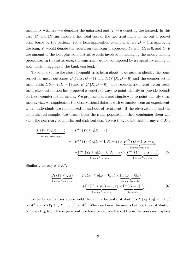
yield the necessary counterfactual distributions. To see this, notice that for any x 2 X 1,

P (Y0 � yjX = x)| {z }known from expt

= P obs (Y0 � yjX = x)

= P obs (Y0 � yjD = 1; X = x)� P obs (D = 1jX = x)| {z }known from obs

+P obs (Y0 � yjD = 0; X = x)| {z }known from obs

� P obs (D = 0jX = x)| {z }known from obs

. (5)

Similarly for any x 2 X 0,

Pr (Y1 � yjx)| {z }known from expt

= Pr (Y1 � yjD = 0; x)� Pr (D = 0jx)| {z }known from obs

+Pr (Y1 � yjD = 1; x)| {z }known from obs

� Pr (D = 1jx)| {z }from obs

. (6)

Thus the two equalities above yield the counterfactual distributions P (Y0 � yjD = 1; x)on X 1 and P (Y1 � yjD = 0; x) on X 0. When we know the means but not the distribution

of Y1 and Y0 from the experiment, we have to replace the c.d.f.�s in the previous displays

9

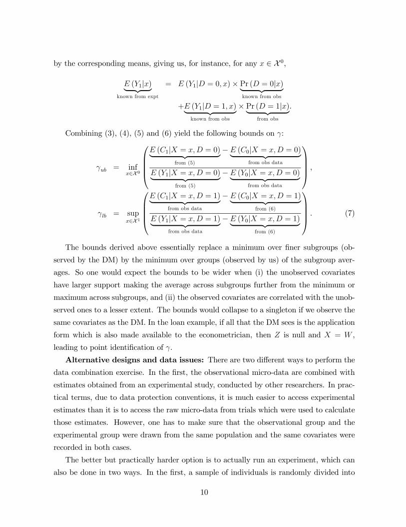
by the corresponding means, giving us, for instance, for any x 2 X 0,

E (Y1jx)| {z }known from expt

= E (Y1jD = 0; x)� Pr (D = 0jx)| {z }known from obs

+E (Y1jD = 1; x)| {z }known from obs

� Pr (D = 1jx)| {z }from obs

.

Combining (3), (4), (5) and (6) yield the following bounds on :

ub = infx2X 0

0BBB@E (C1jX = x;D = 0)| {z }

from (5)

� E (C0jX = x;D = 0)| {z }from obs data

E (Y1jX = x;D = 0)| {z }from (5)

� E (Y0jX = x;D = 0)| {z }from obs data

1CCCA ,

lb = supx2X 1

0BBB@E (C1jX = x;D = 1)| {z }

from obs data

� E (C0jX = x;D = 1)| {z }from (6)

E (Y1jX = x;D = 1)| {z }from obs data

� E (Y0jX = x;D = 1)| {z }from (6)

1CCCA . (7)

The bounds derived above essentially replace a minimum over �ner subgroups (ob-

served by the DM) by the minimum over groups (observed by us) of the subgroup aver-

ages. So one would expect the bounds to be wider when (i) the unobserved covariates

have larger support making the average across subgroups further from the minimum or

maximum across subgroups, and (ii) the observed covariates are correlated with the unob-

served ones to a lesser extent. The bounds would collapse to a singleton if we observe the

same covariates as the DM. In the loan example, if all that the DM sees is the application

form which is also made available to the econometrician, then Z is null and X = W ,

leading to point identi�cation of .

Alternative designs and data issues: There are two di¤erent ways to perform the

data combination exercise. In the �rst, the observational micro-data are combined with

estimates obtained from an experimental study, conducted by other researchers. In prac-

tical terms, due to data protection conventions, it is much easier to access experimental

estimates than it is to access the raw micro-data from trials which were used to calculate

those estimates. However, one has to make sure that the observational group and the

experimental group were drawn from the same population and the same covariates were

recorded in both cases.

The better but practically harder option is to actually run an experiment, which can

also be done in two ways. In the �rst, a sample of individuals is randomly divided into

10

an experimental arm and a non-experimental one. The experimental arm individuals are

randomly assigned to treatment and the observational arm ones are handed over to a DM

who uses his/her discretion. The second way is as follows. First, present all the individ-

uals to the DM and record his recommendations for treatment. This recommendation is

recorded as D = 1 when recommended to have treatment and as D = 0, otherwise. Then

we randomize actual approval across all applications (ignoring the DM�s recommenda-

tion) and observe the outcomes for each individual. The counterfactual P (Y0jD = 1; X)can then be obtained from the outcomes of those who are approved by the DM but were

randomized out of treatment. Conversely for P (Y1jD = 0; X).The experimental approach requires signi�cantly more work to implement but gives

us the ideal set-up where the experimental and observational groups are ex-ante identi-

cal and the same variables can be recorded for both groups. The �rst method, where

experimental results from existing studies are used instead of actually running an exper-

iment, is applicable in many more situations. However, one is somewhat constrained by

the outcomes and covariates that the original researchers had chosen. For the exercise of

inferring risk preferences (see section 5, below) in the case of non-binary outcomes, one

would need the full experimental approach because trial studies rarely report marginal

distributions of Y0 and Y1 (rather than means and medians) which are needed to conduct

this exercise.

3.1 Misallocation

The bounds analysis presented above can be used to test whether there is misallocation

of treatment both within and between demographic groups. To �x ideas, suppose X =

(X1; female) and we are interested in testing if there is treatment misallocation within

males and within females and then we want to test if treatment misallocation between

males and females occurs in a way that hurts, say, females.

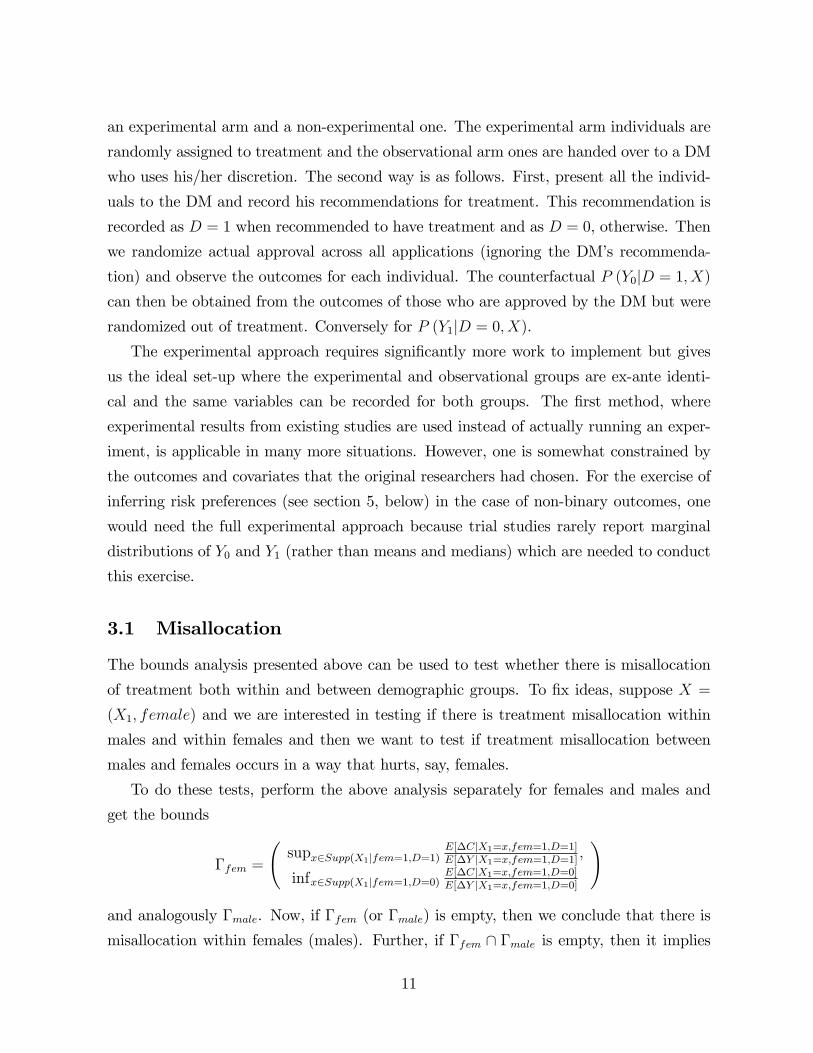
To do these tests, perform the above analysis separately for females and males and

get the bounds

�fem =

supx2Supp(X1jfem=1;D=1)

E[�CjX1=x;fem=1,D=1]E[�Y jX1=x;fem=1,D=1] ;

infx2Supp(X1jfem=1;D=0)E[�CjX1=x;fem=1,D=0]E[�Y jX1=x;fem=1,D=0]

!

and analogously �male. Now, if �fem (or �male) is empty, then we conclude that there is

misallocation within females (males). Further, if �fem \ �male is empty, then it implies

11

that di¤erent thresholds were used for females and males and thus there is misallocation

between males and females.

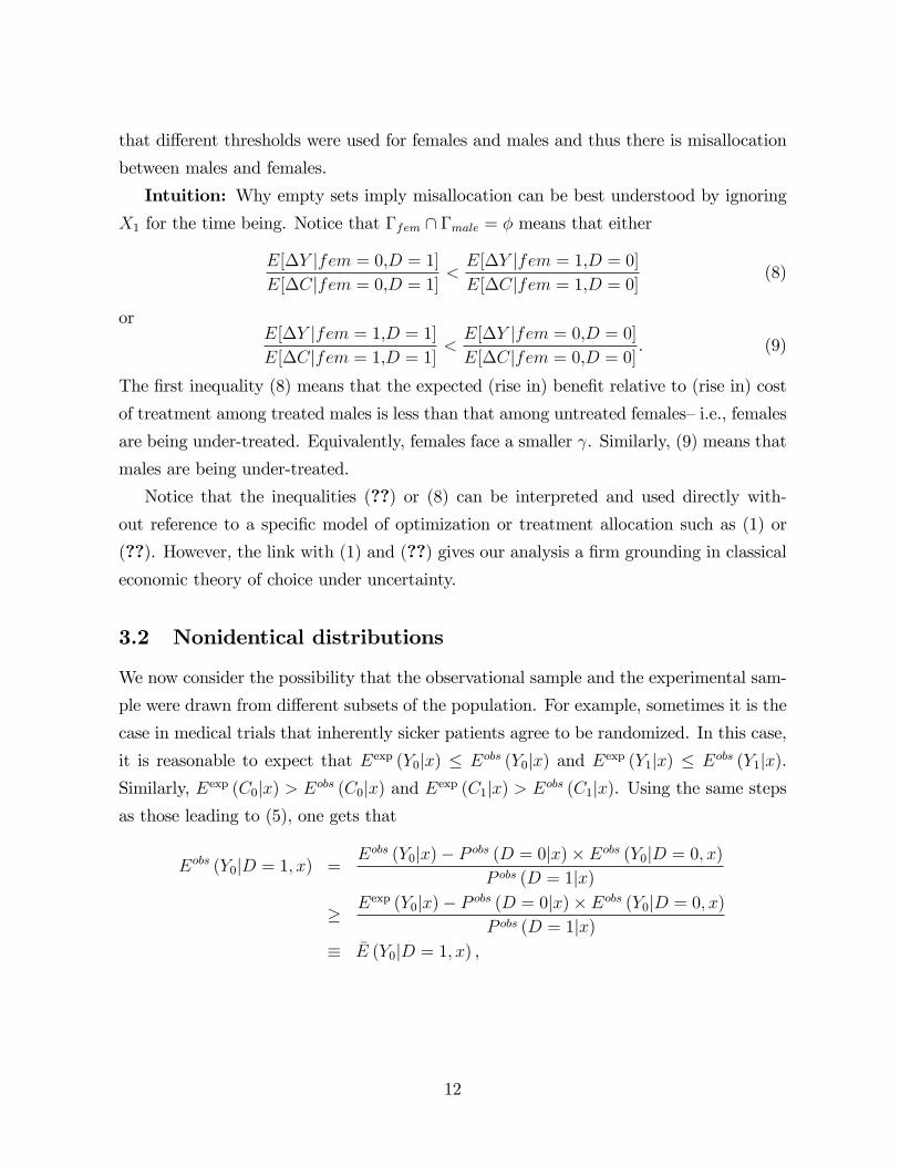
Intuition: Why empty sets imply misallocation can be best understood by ignoring

X1 for the time being. Notice that �fem \ �male = � means that either

E[�Y jfem = 0,D = 1]E[�Cjfem = 0,D = 1]

<E[�Y jfem = 1,D = 0]E[�Cjfem = 1,D = 0]

(8)

orE[�Y jfem = 1,D = 1]E[�Cjfem = 1,D = 1]

<E[�Y jfem = 0,D = 0]E[�Cjfem = 0,D = 0]

. (9)

The �rst inequality (8) means that the expected (rise in) bene�t relative to (rise in) cost

of treatment among treated males is less than that among untreated females�i.e., females

are being under-treated. Equivalently, females face a smaller . Similarly, (9) means that

males are being under-treated.

Notice that the inequalities (??) or (8) can be interpreted and used directly with-

out reference to a speci�c model of optimization or treatment allocation such as (1) or

(??). However, the link with (1) and (??) gives our analysis a �rm grounding in classical

economic theory of choice under uncertainty.

3.2 Nonidentical distributions

We now consider the possibility that the observational sample and the experimental sam-

ple were drawn from di¤erent subsets of the population. For example, sometimes it is the

case in medical trials that inherently sicker patients agree to be randomized. In this case,

it is reasonable to expect that Eexp (Y0jx) � Eobs (Y0jx) and Eexp (Y1jx) � Eobs (Y1jx).Similarly, Eexp (C0jx) > Eobs (C0jx) and Eexp (C1jx) > Eobs (C1jx). Using the same stepsas those leading to (5), one gets that

Eobs (Y0jD = 1; x) =Eobs (Y0jx)� P obs (D = 0jx)� Eobs (Y0jD = 0; x)

P obs (D = 1jx)

� Eexp (Y0jx)� P obs (D = 0jx)� Eobs (Y0jD = 0; x)P obs (D = 1jx)

� �E (Y0jD = 1; x) ,

12

and similarly,

Eobs (Y1jD = 0; x) =Eobs (Y1jx)� P obs (D = 0jx)� Eobs (Y1jD = 0; x)

P obs (D = 1jx)

� Eexp (Y1jx)� P obs (D = 0jx)� Eobs (Y1jD = 0; x)P obs (D = 1jx)

� �E (Y1jD = 0; x) .

The quantities �E (Y1jD = 0; x) and �E (Y0jD = 1; x) are clearly identi�ed. An analogousset of inequalities hold with Y replaced by C and the inequality sign reversed (since the

experimental group, being sicker will be more expensive to treat). These bounds can be

used to detect misallocation. For instance, if it is the case that

Eobs (Y1jD = 1;male)� �E (Y0jD = 1;male)Eobs (C1jD = 1;male)� �E (C0jD = 1;male)

��E (Y1jD = 0; female)� Eobs (Y0jD = 0; female)�E (C1jD = 0; female)� Eobs (C0jD = 0; female)

, (10)

then it follows that

1

male<

Eobs (�Y jD = 1;male)Eobs (�CjD = 1;male)

� Eobs (Y1jD = 1;male)� �E (Y0jD = 1;male)Eobs (C1jD = 1;male)� �E (C0jD = 1;male)

��E (Y1jD = 0; female)� Eobs (Y0jD = 0; female)�E (C1jD = 0; female)� Eobs (C0jD = 0; female)

� Eobs (�Y jD = 0; female)Eobs (�CjD = 0; female)

� 1

fem.

Thus, female is smaller, meaning that the outcomes of females are being weighed less

relative to males. However, since (10) implies (8), it will be harder to detect misallocation

here compared to when the experimental and observational data came from identical

populations.

3.3 Selection on observables

In some situations, a researcher may have access to exactly the same set of covariates

W that the DM had observed prior to making the decision. Examples include postal

13

application for credits or student admissions where applications are scored anonymously.

Even when the application process involves a face-to-face interview but the interview score

is available, the same set-up applies. In this case, the threshold is point-identi�ed:

supw

E [�CjD = 1;W = w]

E [�Y jD = 1;W = w]= = inf

w

E [�CjD = 0;W = w]

E [�Y jD = 0;W = w].

Notice that when there is a tie (which may happen if the X�s are discrete) and it is broken

via randomization within the marginal group, the supremum and in�mum will be attained

at multiple values of W but they would still be equal. For example, suppose W 2 f0; 1g,and is such that

4 Alternative mechanisms leading to misallocation

We now discuss three alternative allocation mechanisms which can potentially lead to

empty identi�ed sets and thus suggest misallocation. We de�ne and make the distinc-

tion between wilful or prejudicial discrimination, inadvertent discrimination and implicit

discrimination�all of which will lead to misallocation that we can potentially detect with

our bounds-based analysis. Instead of presenting general models, we describe speci�c

scenarios to outline the subtleties which make it hard to move from detection of misallo-

cation to discerning its source. For simplicity of exposition, we will assume that �C is a

constant k (i.e., does not vary with any component of W ), so that the optimal decision

criterion will be

D = 1() E (�Y jW ) > �,

where � = k= .

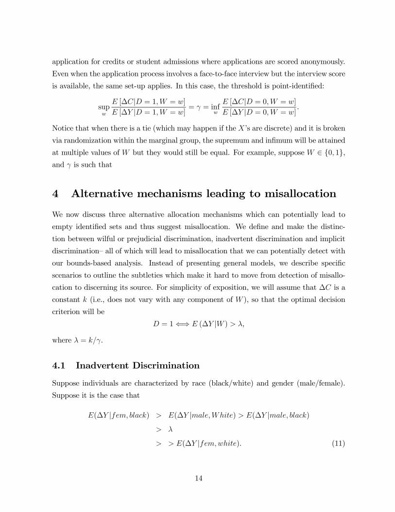
4.1 Inadvertent Discrimination

Suppose individuals are characterized by race (black/white) and gender (male/female).

Suppose it is the case that

E(�Y jfem; black) > E(�Y jmale;White) > E(�Y jmale; black)

> �

> > E(�Y jfem;white). (11)

14

Suppose that the fraction of whites among women is high enough that

E(�Y jmale) > � > E(�Y jfemale). (12)

That is, black females bene�t a lot from treatment while while females bene�t the least.

If white females are a much larger group than black females, then on average, females

bene�t less from treatment and hence (12) holds.

Now suppose the DM ignores race and allocates treatment, based only on gender.

Then D = 1 i¤ the individual is male and so it must be the case that

E(�Y jD = 0; Black)

= E(�Y jfemale; Black)

> E(�Y jmale;White), by (11)

= E(�Y jD = 1;White).

Thus, we would conclude that there is misallocation which works against blacks precisely

because the DM is race-blind in his decision-making.

Notice that this violates a key assumption we started with, viz., that the DM uses all

covariates that we observe plus possibly more. Here we observe race but the DM does not

take into account race in making the allocation. This works against black females because

they are treated the same as white females because of their gender and the inability or

unwillingness of the DM to condition on race. The scenario described above is quite stark

in that we are detecting misallocation by race precisely because the DM is not taking race

into account in making the allocation. It would thus be dramatically wrong to conclude

from (??) that there is prejudice against blacks. Notice that this "mistake" is very di¤erent

from and more subtle than the mistake of interpreting statistical discrimination as taste-

based discrimination.

4.2 Wilful Discrimination

This is the simplest case where di¤erent thresholds are being used for the di¤erent de-

mographic groups. In our gender example above, females are discriminated against if

�fem > �male. Notice that such wilful discrimination has no implications for the rate

of treatment in the two groups. That is, it is certainly possible that �fem = �male

and Pr (D = 1jfem = 0) > Pr (D = 1; fem = 1). Conversely, it is also possible that

15

�fem > �male but Pr (D = 1jfem = 0) � Pr (D = 1; fem = 1). Whether the rate of treat-

ment is equal across demographic groups depends on the fraction of individuals within

that group whose expected bene�ts from treatment are above the threshold for that group.

So an e¢ cient allocation, using a common threshold for all demographic groups, may be

one where a larger fraction of males are treated if a larger fraction of males have expected

bene�ts from treatment above the common threshold than females.

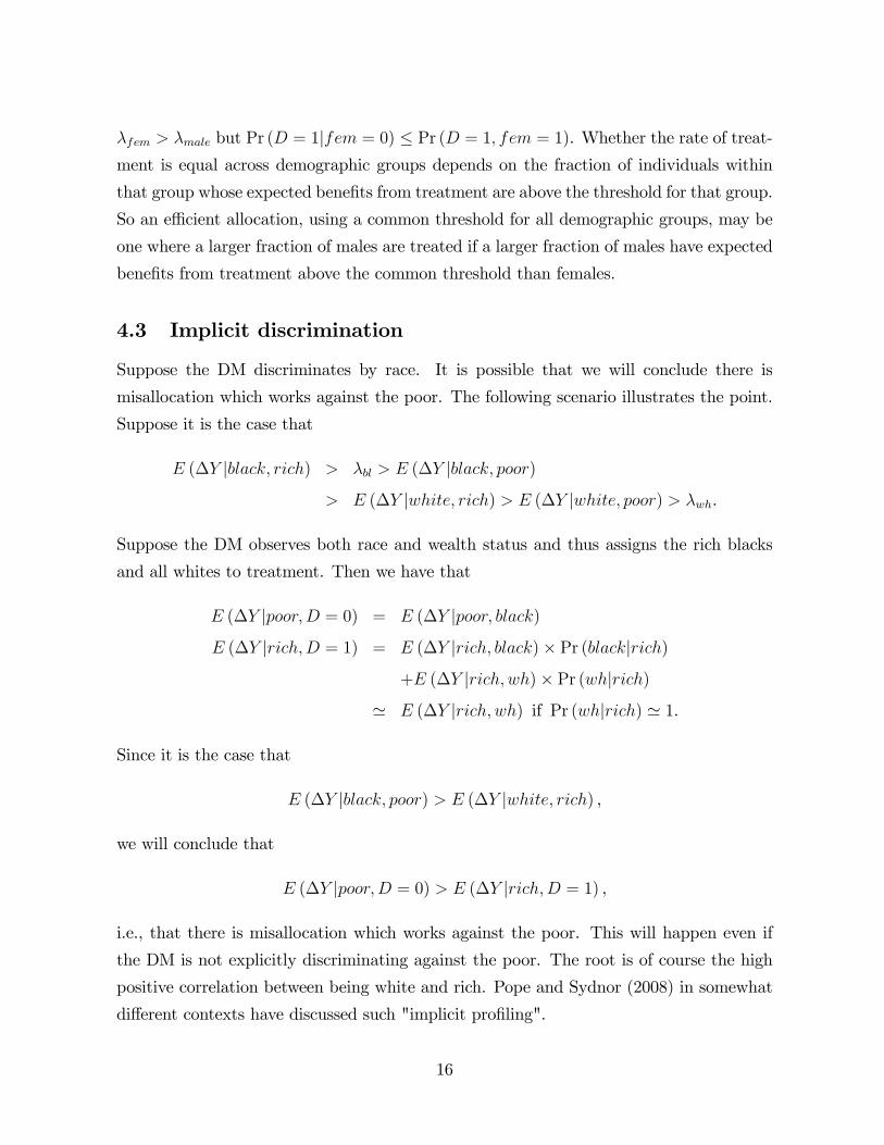
4.3 Implicit discrimination

Suppose the DM discriminates by race. It is possible that we will conclude there is

misallocation which works against the poor. The following scenario illustrates the point.

Suppose it is the case that

E (�Y jblack; rich) > �bl > E (�Y jblack; poor)

> E (�Y jwhite; rich) > E (�Y jwhite; poor) > �wh.

Suppose the DM observes both race and wealth status and thus assigns the rich blacks

and all whites to treatment. Then we have that

E (�Y jpoor;D = 0) = E (�Y jpoor; black)

E (�Y jrich;D = 1) = E (�Y jrich; black)� Pr (blackjrich)

+E (�Y jrich; wh)� Pr (whjrich)

' E (�Y jrich; wh) if Pr (whjrich) ' 1.

Since it is the case that

E (�Y jblack; poor) > E (�Y jwhite; rich) ,

we will conclude that

E (�Y jpoor;D = 0) > E (�Y jrich;D = 1) ,

i.e., that there is misallocation which works against the poor. This will happen even if

the DM is not explicitly discriminating against the poor. The root is of course the high

positive correlation between being white and rich. Pope and Sydnor (2008) in somewhat

di¤erent contexts have discussed such "implicit pro�ling".

16

In all three cases listed above, we would potentially detect misallocation based on some

covariate(s). However, this misallocation could be a result of prejudicial discrimination

based on that particular covariate, inadvertent discrimination from ignoring that covariate

in the allocation or implicit discrimination on a positively correlated covariate. While the

exact form of discrimination cannot be pinpointed, one can conclude that there has been

misallocation of treatment, leading some demographic groups to receive less and some

others to receive more amounts of treatment than what economic e¢ ciency would dictate.

In our terminology, the former group has been subjected to non-statistical discrimination.

5 Broadening the model

We now extend the analysis to include risk averse behavior by the DM and transform the

problem of detecting misallocation for a speci�c outcome to the problem of detecting the

extent of risk aversion which justify the observed allocation as an e¢ cient one.

5.1 Risk Aversion: Parametric

In this part of the analysis we ask what risk-averse utility function(s) are consistent with

e¢ cient allocation, given the data. To do this we consider a family of risk averse utility

functions u (�; �), indexed by a �nite dimensional parameter � and the correspondingallocation rule which is a generalization of (??)

D = 1 i¤E (u (Y1; �) jX;Z)� E (u (Y0; �) jX;Z)

E (C1jX;Z)� E (C0jX;Z)> �. (13)

Examples of such utility functions are CRRA u (Y; �) � Y 1��

1�� for � 2 (0; 1) and CARAu (Y; �) � �e�Y for � � 0. Let �Y (�) � u (Y1; �)� u (Y0; �).When the DM�s subjective expectations are consistent with true distributions in the

population, we have that

E (u (Y1; �) jX;D = 1)� E (u (Y0; �) jX;D = 1)E (C1jX;D = 1)� E (C0jX;D = 1)

> �, w.p.1.

As before, we do the analysis separately for males and females to get the bounded sets in

terms of �:

[Lf (�) ; Uf (�)] =

8>><>>:0BB@

supx2Supp(X1jfem=1;D=0)E[�Y (�)jX1=x;fem=1,D=0]E[�CjX1=x;fem=1,D=0]

< �

� infx2Supp(X1jfem=1;D=1)E[�Y (�)jX1=x;fem=1,D=1]E[�CjX1=x;fem=1,D=1]

1CCA9>>=>>;

17

and similarly, [Lm (�) ; Um (�)].

So the values of � which are consistent with e¢ cient allocation within gender are the

ones for which

Lf (�) � Uf (�) and Lm (�) � Um (�) . (14)

Further, the values of � which are consistent with e¢ cient allocation across demographic

groups are the ones for which

max fLf (�) ; Lm (�)g � min fUf (�) ; Um (�)g . (15)

If the set of � � 0 for which both (14) and (15) hold turns out to be empty, then no memberof the corresponding family of utility functions will justify the observed allocation as an

e¢ cient one.

5.2 Risk Aversion: nonparametric

Now consider a general di¤erentiable Bernoulli utility function u (�) which will be theingredient of a VnM utility de�ned over lotteries. In order for such a utility function to

rationalize the observed treatment choice, we must have that for all x; x0

E [u (Y1)� u (Y0) jD = 1; X = x]

E [�CjD = 1; X = x]� E [u (Y1)� u (Y0) jD = 0; X = x0]

E [�CjD = 0; X = x0]. (16)

Here, we focus on the case where both Y and X are discrete. The continuous case is

treated as a separate subsection. So assume that Y1 and Y0 are discrete, with union

support equal to fa1:::amg.The above condition reduces to: for all x; x0:mXj=1

u (aj)

�Pr (Y1 = ajjx;D = 1)� Pr (Y0 = ajjx;D = 1)

E [C1 � C0jD = 1; X = x]

�| {z }

=h1(aj ;x), say

�mXj=1

u (aj)

�Pr (Y1 = ajjx; ;D = 0)� Pr (Y0 = ajjx0; D = 0)

E [C1 � C0jD = 0; X = x; ]

�| {z }

h0(aj ;x0), say

.

18

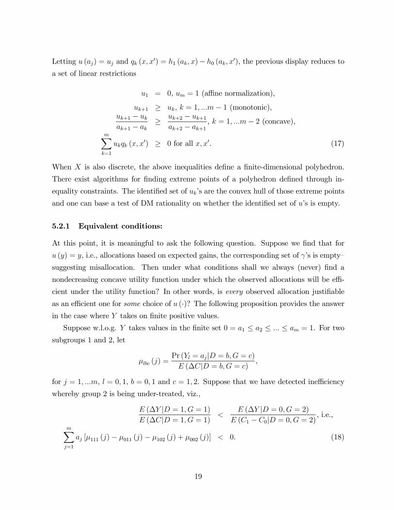
Letting u (aj) = uj and qk (x; x0) = h1 (ak; x)� h0 (ak; x0), the previous display reduces toa set of linear restrictions

u1 = 0, um = 1 (a¢ ne normalization),

uk+1 � uk, k = 1; :::m� 1 (monotonic),uk+1 � ukak+1 � ak

� uk+2 � uk+1ak+2 � ak+1

, k = 1; :::m� 2 (concave),mXk=1

ukqk (x; x0) � 0 for all x; x0. (17)

When X is also discrete, the above inequalities de�ne a �nite-dimensional polyhedron.

There exist algorithms for �nding extreme points of a polyhedron de�ned through in-

equality constraints. The identi�ed set of uk�s are the convex hull of those extreme points

and one can base a test of DM rationality on whether the identi�ed set of u�s is empty.

5.2.1 Equivalent conditions:

At this point, it is meaningful to ask the following question. Suppose we �nd that for

u (y) = y, i.e., allocations based on expected gains, the corresponding set of �s is empty�

suggesting misallocation. Then under what conditions shall we always (never) �nd a

nondecreasing concave utility function under which the observed allocations will be e¢ -

cient under the utility function? In other words, is every observed allocation justi�able

as an e¢ cient one for some choice of u (�)? The following proposition provides the answerin the case where Y takes on �nite positive values.

Suppose w.l.o.g. Y takes values in the �nite set 0 = a1 � a2 � ::: � am = 1. For twosubgroups 1 and 2, let

�lbc (j) =Pr (Yl = ajjD = b;G = c)E (�CjD = b;G = c) ,

for j = 1; :::m, l = 0; 1, b = 0; 1 and c = 1; 2. Suppose that we have detected ine¢ ciency

whereby group 2 is being under-treated, viz.,

E (�Y jD = 1; G = 1)E (�CjD = 1; G = 1) <

E (�Y jD = 0; G = 2)E (C1 � C0jD = 0; G = 2)

, i.e.,

mXj=1

aj [�111 (j)� �011 (j)� �102 (j) + �002 (j)] < 0. (18)

19

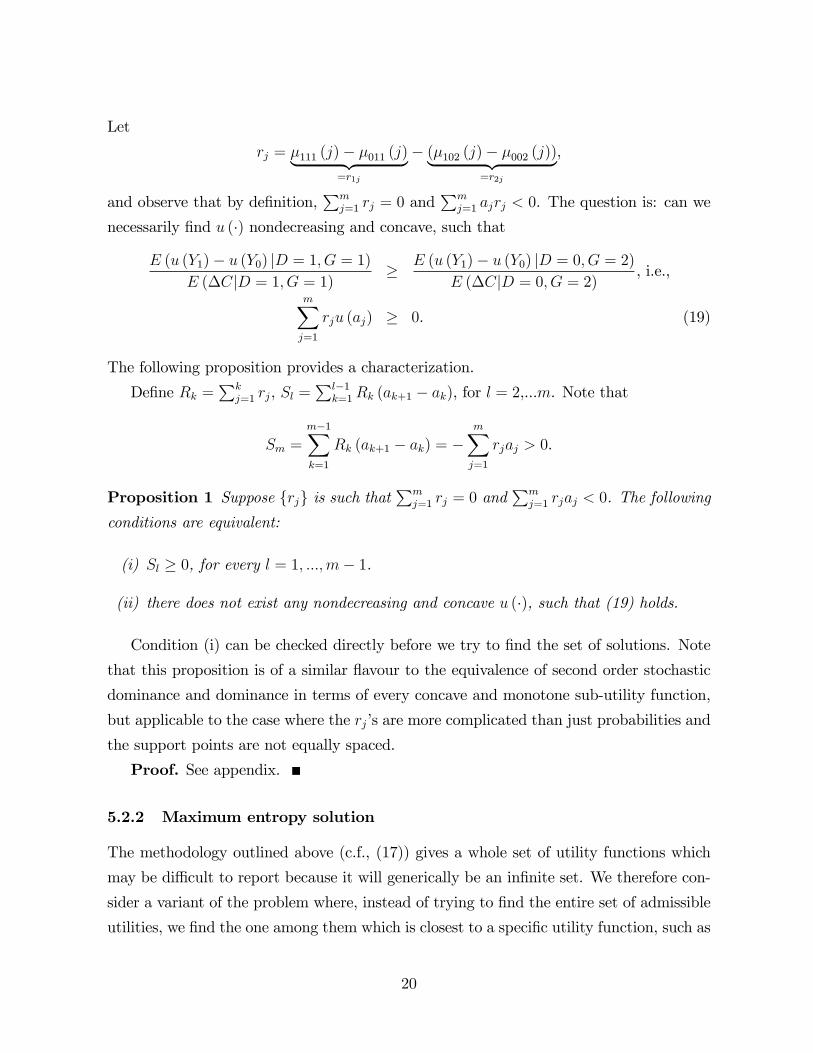
Let

rj = �111 (j)� �011 (j)| {z }=r1j

� (�102 (j)� �002 (j))| {z }=r2j

,

and observe that by de�nition,Pm

j=1 rj = 0 andPm

j=1 ajrj < 0. The question is: can we

necessarily �nd u (�) nondecreasing and concave, such that

E (u (Y1)� u (Y0) jD = 1; G = 1)E (�CjD = 1; G = 1) � E (u (Y1)� u (Y0) jD = 0; G = 2)

E (�CjD = 0; G = 2) , i.e.,

mXj=1

rju (aj) � 0. (19)

The following proposition provides a characterization.

De�ne Rk =Pk

j=1 rj, Sl =Pl�1

k=1Rk (ak+1 � ak), for l = 2,...m. Note that

Sm =m�1Xk=1

Rk (ak+1 � ak) = �mXj=1

rjaj > 0.

Proposition 1 Suppose frjg is such thatPm

j=1 rj = 0 andPm

j=1 rjaj < 0. The following

conditions are equivalent:

(i) Sl � 0, for every l = 1; :::;m� 1.

(ii) there does not exist any nondecreasing and concave u (�), such that (19) holds.

Condition (i) can be checked directly before we try to �nd the set of solutions. Note

that this proposition is of a similar �avour to the equivalence of second order stochastic

dominance and dominance in terms of every concave and monotone sub-utility function,

but applicable to the case where the rj�s are more complicated than just probabilities and

the support points are not equally spaced.

Proof. See appendix.

5.2.2 Maximum entropy solution

The methodology outlined above (c.f., (17)) gives a whole set of utility functions which

may be di¢ cult to report because it will generically be an in�nite set. We therefore con-

sider a variant of the problem where, instead of trying to �nd the entire set of admissible

utilities, we �nd the one among them which is closest to a speci�c utility function, such as

20

the risk neutral one u (y) = y or a speci�c risk-averse one, e.g., u (y) =py. This objective

can be achieved through the use of entropy maximization, which we describe now.

Recall the constraints (17). De�ne v1 = u1 = 0 and vk = uk � uk�1 for k = 2; :::K. Inmatrix notation, 266664

v1

v2

:::

vk

377775| {z }

v

=

266666664

1 0 0 ::: 0

�1 1 0 ::: 0

0 �1 1 0::: 0

: : : : :

0 ::: 0 �1 1

377777775| {z }

S

266664u1

u2

:::

uk

377775| {z }

,

where S is nonsingular. Also, for �xed x, x0, let q (x; x0) denote the k-vector whose kth

entry is qk (x; x0). Then the constraints (17) can be rewritten as

vk � 0, k = 1; :::K � 1,kXk=1

vk = 1,

vkak � ak�1

� vk+1ak+1 � ak

, k = 1; :::K � 1

v0�S�1q (x; x0)

�� 0 for all x; x0. (20)

Given the form of the constraints, one can apply the principle of maximum entropy and

solve

max

(�

KXk=1

�vk

ak � ak�1

�ln

�vk

ak � ak�1

�), s.t. (20).

If there were no q-constraints, then the solution would be vk = ak�ak�1. This correspondsto the risk-neutral situation u (a) = a. Therefore maximizing the entropy s.t. the con-

straints corresponds to �nding the most risk-neutral u (�) which satis�es the constraints.Standard software can be used to perform these calculations since the problem is strictly

concave. Once the v�s are obtained, one can �nd the corresponding u�s by using u = S�1v.

To get the utility function closest to u (y) =py, one would solve

max

(�

KXk=1

vkpak �

pak�1

ln

�vkp

ak �pak�1

�), s.t. (20).

In the absence of the q-constraints, the solution would be vk =pak �

pak�1, i.e. u (y) =

py, as desired.

21

In contrast to the set-identi�ed situation, the maximum entropy problem will either

have no solution (if the constraint set is empty, for instance) or a unique solution, which

would make it easy to report. This unique solution will have a meaningful interpretation

as the admissible utility function closest to a speci�c utility function (e.g., a risk-neutral

one). Moreover, when the q�s are estimated, one can, in principle, construct con�dence

intervals for both the solution and the value function for the above problems, using the

distribution theory for the estimated q�s.

5.2.3 Inference

Testing whether the existing allocation is e¢ cient for a given utility function, reduces

essentially to testing a set of (conditional) moment inequalities (c.f., (8) or (9) above).

There is an existing and expanding literature in econometrics, dealing with such tests.

For example, one can adopt the method of Andrews and Soares (2009) to conduct such

tests and calculate con�dence intervals for the di¤erence in treatment thresholds between

demographic groups. This corresponds to inference on the true parameters, rather than

inference on the identi�ed set.

Inferring utility parameters consistent with e¢ cient allocation is an estimation problem

where the parameters of interest are de�ned via conditional moment inequalities. The test

of rationality thereof is analogous to speci�cation testing in GMM problems but now with

inequality constraints. For the parametric case or the nonparametric case with discrete

outcome and covariates, the utility parameters are �nite-dimensional and we are interested

in inferring the entire feasible set of utility parameters. So inference can be conducted

using, e.g., CHT (2005). Tests of rationality again amount to checking emptiness of

con�dence sets, which can be done using Andrews and Soares.

Inference for the maximum entropy solution, to our knowledge, is nonstandard. Es-

sentially, the inference problem is to �nd the distribution theory for the solution and value

22

function for the problem

max

(�

KXk=2

vk ln (vk)

), s.t.

vk � 0, k = 2; :::K,KXk=1

vk = 1,

vkak � ak�1

� vk+1ak+1 � ak

, k = 2; :::K � 1

v0�S�1q (x; x0)

�� 0 for all x; x0. (21)

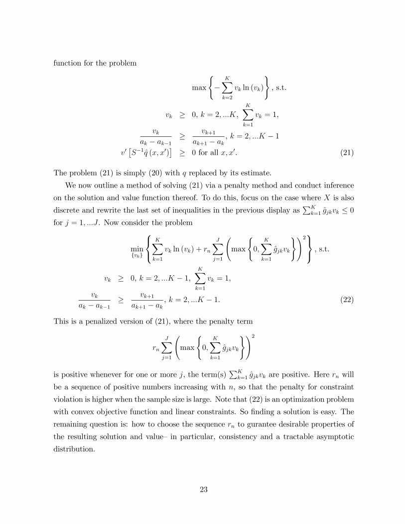
The problem (21) is simply (20) with q replaced by its estimate.

We now outline a method of solving (21) via a penalty method and conduct inference

on the solution and value function thereof. To do this, focus on the case where X is also

discrete and rewrite the last set of inequalities in the previous display asPK

k=1 gjkvk � 0for j = 1; :::J . Now consider the problem

minfvkg

8<:KXk=1

vk ln (vk) + rn

JXj=1

max

(0;

KXk=1

gjkvk

)!29=; , s.t.vk � 0, k = 2; :::K � 1,

KXk=1

vk = 1,

vkak � ak�1

� vk+1ak+1 � ak

, k = 2; :::K � 1. (22)

This is a penalized version of (21), where the penalty term

rn

JXj=1

max

(0;

KXk=1

gjkvk

)!2

is positive whenever for one or more j, the term(s)PK

k=1 gjkvk are positive. Here rn will

be a sequence of positive numbers increasing with n, so that the penalty for constraint

violation is higher when the sample size is large. Note that (22) is an optimization problem

with convex objective function and linear constraints. So �nding a solution is easy. The

remaining question is: how to choose the sequence rn to gurantee desirable properties of

the resulting solution and value� in particular, consistency and a tractable asymptotic

distribution.

23

De�ne

Qn (v) =

8<:KXk=1

vk ln (vk) + rn

JXj=1

max

(0;

KXk=1

gjkvk

)!29=; ,Q (v) =

KXk=1

vk ln (vk) ,

A =

(v : vk � 0, k = 2; :::K,

PKk=1 vk = 1,

vkak�ak�1 �

vk+1ak+1�ak , k = 2; :::K � 1.

),

B =

(v :

KXk=1

gjkvk � 0, j = 1; :::J).

We use the standard convention that vk ln (vk) = 0 if vk = 0.

Proposition 2 (Consistency) Assume thatpnvec (g � g) N (0;�). Choose rn such

that rn = op (pn) and rn !1 as n!1. Then

p limn!1

�argmin

v2AQn (v)

�= arg min

v2A\BQ (v) .

Proof. See appendix.

Corollary 1 (Consistency of value function) Under the same conditions, as the pre-

vious proposition,

p limn!1

�Qn

�argmin

v2AQn (v)

��= Q

�arg min

v2A\BQ (v)

�:

Proof. See appendix.

5.3 Continuous case

Inequalities: When Y is continuously distributed with support [0; 1], the condition (16)

reduces to Zu (y)

�pY1 (yjx;D = 1)� pY0 (yjx;D = 1)

E [C1 � C0jD = 1; X = x]

�| {z }

=h1(y;x), say

dy

�Zu (y)

�pY1 (yjx0; D = 0)� pY0 (yjx0; D = 0)

E [�CjD = 0; X = x0]

�| {z }

h0(y;x0), say

dy.

24

So the question is: does there exist a function u (:) s.t.

u (0) = 0, u(1) = 1 (a¢ ne normalization)

u0 (�) � 0 (monotonic)

u00 (�) � 0 (concave)Zu (y)h1 (y; x) dy �

Zu (y)h0 (y; x

0) dy for all x; x0.

Maximum Entropy: De�ne v (y) = u0 (y) and

H (a;x; x0) �Z a

0

[h1 (y; x)� h0 (y; x0)] dy.

Then the constraints (16) reduce to

v (y) � 0,Z 1

0

v (y) dy = 1

�v0 (y) � 0 for all y 2 [0; 1]

�Zv (y)H (y;x; x0) dy � 0 for all x; x0. (23)

The last inequality follows by applying integration by parts toRu (y) [h1 (y; x)� h0 (y; x0)] dy

and recognizing that for any x, it follows from de�nition of the h functions thatR 10h1 (y; x) dy =

0. The maximum entropy solution is then given by

max�Z 1

0

v (y) ln

�v (y)

v0 (y)

�dy, s.t. (23),

where v0 (y) corresponds to a reference utility function. For example, when v0 (y) = 1 we

�nd the most risk-neutral utility function satisfying the constraints whereas v0 (y) = 1=y

corresponds to �nding the utility function closest to the risk-averse sub-utility u (y) =

ln (y) which satis�es the constraints.

Inference: Consider the case where Y is continuous and recall the restrictions:

u (0) = 0, u(1) = 1 (a¢ ne normalization)

u0 (�) � 0 (monotonic)

u00 (�) � 0 (concave)Zu (y)h1 (y; x) dy �

Zu (y)h0 (y; x

0) dy for all x; x0.

25

SupposeX is discrete and takes values a1; :::aK . Let hjk (y) � h1 (y; aj)�h0 (y; ak). De�nethe criterion function as

Q (u) =Xj

Xk

�min

�0;

Zu (y)hjk (y) dy

��2and its estimated analog (with hjk (�) replaced by their estimates) as Qn (u). At this point,it is necessary to approximate the functions u (�) via a basis (a sieve) and imposing therestrictions implied by the structure of utility functions and the e¢ ciency requirement.

Typically, we would consider a sieve basis fp1; :::; pJng and consider approximatingu (�) by the sum

PJnl=1 �lpl (�) and choosing the coe¢ cients such that the monotonicity

and concavity are satis�ed. One convenient choice of basis are cardinal B-splines (see,

Chen (2005)) for which monotonicity and concavity are equivalent to the coe¢ cients f�lg,l = 1; 2; :::, satisfying simple linear inequalities�say, A(Jn)� � 0, for an appropriate matrixA(Jn). Then the identi�ed set for u (�) can be approximated by the identi�ed set for the�-coe¢ cients. The latter can be obtained by using the criterion function

~Qn (�) =Xj

Xk

min

(0;

Z ( JnXl=1

�lpl (y)

)hjk (y) dy

)!2

and its estimated analog (with hjk (�) replaced by their estimates) denoted by �Qn (�). TheCI for the identi�ed set of approximating ��s is then given by

Cn =n� : A(Jn)� � 0; �Qn (�) � c�

o,

for an appropriately chosen c�. A detailed analysis is left to future research.

The maximum entropy solution corresponding to the sample values of q (x; x0) will be

random simply because the are estimated. Finding the asymptotic distribution of the

resulting v�s would require us to �rst decide on which constraints are (approximately)

binding. One approach is to �rst calculate the sample solution for the v�s by solving the

optimization problem with the estimated value of q (x; x0). Then drop those constraints

for which the the constraint function evaluated at the sample estimates of the v�s exceeds

�n�a decreasing function of the sample size n (such as ln (n)�1=2). These are the esti-

mated nonbinding constraints with zero Lagrange multipliers and these will not appear in

the �nal solution. Then use the remaining constraints to solve the optimization problem

explicitly, resulting in a set of �rst order equations involving (possibly nonlinearly) the

26

v�s, the Lagrange multipliers for the binding constraints and the q�s. Finding the asymp-

totic distribution of the resulting estimated v�s will simply be an application of the delta

method. The only nontrivial issue involves �guring out how the �rst stage decision on

which constraints are binding will impact the asymptotic distribution of the estimated

v�s. It is reasonable to expect that when the �rst-stage cut-o¤ is chosen to be of higher

order than n�1=2, the �rst stage decision has no impact on the asymptotic distribution,

i.e., it is as if we knew which constraints bind.

6 A simulation exercise

We report simulation results for the following linear regression model linking outcome Y

with regressors Z; f and the treatment indicator D as follows.

Y = 1 + 0:2Z + � �DZ + 0:4f + 0:5Df

E (�Y jZ; f) = � � Z + 0:5� f .

We generate (Z; f �) from a bivariate normal with mean zero, correlation 0:5 and variances

(�2z; 1). The coe¢ cient � is chosen to be positive. The variable f is a dummy for female

and is generated as the indicator for f � > 0. We generate 2N observations this way and

randomly divide them into an observational and an experimental group.

Within the experimental group, the binary treatment D was generated randomly.

Corresponding to a realization of (D;Z; f), the corresponding Y was generated according

to the model.

In the observational group, the DM was assumed to calculate E (Y jZ; f;D = 1) andE (Y jZ; f;D = 0) using the actual model coe¢ cients and then assign the males (f = 0) totreatment if the di¤erence exceeds male = 0 and assign the females (f = 1) to treatment

if the di¤erence exceeds fem = 0:5. Given the model, this means that for both males

and females, D = 1 i¤ Z > 0.

In both the experimental and observational samples, the econometrician observes f; Y

but not Z. Additionally, the econometrician observes a noisy signal of Z. This is given by

the variable X = 1+ 1 (�Z + � > 0) with "~N (0; 1). The DM�s rule implies the following

27

expressions.

E (�Y jD = 1; f = 1; X = x) = � � E fZjZ > 0; f = 1; X = xg+ 0:5,

E (�Y jD = 0; f = 1; X = x) = � � E fZjZ < 0; f = 1; X = xg+ 0:5,

E (�Y jD = 1; f = 0; X = x) = � � E fZjZ > 0; f = 0; X = xg ,

E (�Y jD = 0; f = 0; X = x) = � � E fZjZ < 0; f = 0; X = xg .

The true bounds are then given by

maxx2f1;2g

� � E fZjZ < 0; f = 1; X = xg+ 0:5

� f

� minx2f1;2g

� � E fZjZ > 0; f = 1; X = xg+ 0:5,

and

maxx2f1;2g

� � E fZjZ < 0; f = 0; X = xg

� m

� minx2f1;2g

� � E fZjZ > 0; f = 0; X = xg ,

and these can be easily simulated.

The values of �, � and variance of Z were varied in the experiment. A larger absolute

value of � indicates that observing X rather than Z is less of a handicap and so this

should lead to narrower bounds on the thresholds. A larger �2z implies wider support

for Z, which, ceteris paribus, will widen the bounds because it would lead to a larger

di¤erence between the minimum (or maximum) over the support of Z and the mean over

the distribution of Z. Bounds will be narrower when � is close to zero. The intuition

is that when � is close to zero, the omitted variable Z plays a smaller role in treatment

assignment and not knowing Z is less of a handicap for knowing f and m.

For each sample size and each choice of �, �, �2z, we ran 100 replications of the

experiment. In each replication, we calculated sample-based bounds on male and femand constructed con�dence intervals for the di¤erence fem � male , using the stepsoutlined in section 3. We report two sets of bounds�one that is simply the sample analog

of the population inequalities and the other is a weighted average of bounds across values

ofX where weight equals the inverse of the square-root of p�(1� p) and p is the probability

28

in the observational sample that D = 1 for that value of X. The results are shown in

table 1.

Second, we calculated bounds on the risk aversion parameter corresponding to the

parametric case. Third, we calculated bounds on the (monotone and concave) utility

functions corresponding to the nonparametric case. One would expect the test to reject

rationality more often and the bounds to be narrower when the sample size is large.

7 Conclusion

Alternatives

Get DM�s decision on applications but randomize�cleanest

Randomized allocation followed by DM�s allocation�e.g. students into classes

TBA...

References

[1] Andrews and Soares

[2] Bertrand, Marianne and Mullainathan, Sendhil (2002). ""Are Emily and Jane More

Employable than Lakisha and Jamal? A Field Experiment on Labor Market Dis-

crimination,"". American Economic Review 94: 991.

[3] Bhattacharya & Dupas (2010): Inferring E¢ cient Treatment Assignment under Bud-

get Constraints", NBER working paper number

[4] Chandra and Staiger (2009): Identifying Provider Prejudice

in Healthcare," manuscript, March 2008, downloadable from:

http://www.hks.harvard.edu/fs/achandr/Provider%20Prejudice%204March%202008.pdf

[5] Chernozhukov, Hong and Tamer

[6] Elliott, Komunjer and Timmerman (2005): Estimation and Testing of Forecast Ra-

tionality under Flexible Loss. Review of Economic Studies, 72, pp. 1107-1125.

[7] Goldin, Claudia and Rouse, Cecilia (2000): "Orchestrating Impartiality", The Amer-

ican Economic Review, 90(4), pp. 715 - 41.

29

[8] Heckman, J. (1998): Journal of Economic Perspectives-Volume 12, Number 2, Pages

101-116.

[9] Knowles, Persico and Todd (2001): Racial Bias in Motor Vehicle Searches: Theory

and Evidence, Journal of Political Economy, 2001 V109 (11) pages 203-229.

[10] Manski, C. F. (1990): Nonparametric Bounds on Treatment E¤ects, The American

Economic Review, Vol. 80, No. 2, pp. 319-323.

[11] Patton, Andrew J. & Timmermann, Allan (2007): "Testing Forecast Optimality

Under Unknown Loss," Journal of the American Statistical Association, vol. 102,

pages 1172-1184.

[12] Persico, N (2009): "Racial Pro�ling? Detecting Bias Using Statistical Evidence",

Annual Review of Economics, volume 1.

8 Appendix: Proofs

Derivation of (1): The solution to the problem

maxA

�Z1 fw 2 Ag y1dP subY1;W

(y1; w) +

Z1 fw 2 Acg y0dP subY0;W

(y0; w)

�s.t. Z

1 fw 2 Ag c1dP subC1;W(c1; w) +

Z1 fw 2 Acg c0dP subC0;W

(c0; w) � c,

is of the form A� = fw : � (w) < g, with

� (w) � Esub (�CjW = w)

Esub (�Y jW = w); c =

Zw2w

1 (� (w) < ) dP subW (w) .

Proof. The welfare resulting from a generic choice of A, satisfying the budget con-

30

straint, di¤ers from the welfare from using A� by an amount given by

G (A)�G (A�)

=

Z1 fw 2 Ag y1dP subY1;W

(y1; w) +

Z1 fw 2 Acg y0dP subY0;W

(y0; w)

��Z

1 fw 2 A�g y1dP subY1;W(y1; w) +

Z1 fw 2 A�cg y0dP subY0;W

(y0; w)

�=

Z "1 fw 2 Ag � 1 fw 2 A�cg�1 fw 2 A�g � 1 fw 2 Acg

#y1dP

subY1;W

(y1; w)

+

Z "1 fw 2 Acg � 1 fw 2 A�g�1 fw 2 Ag � 1 fw 2 A�cg

#y0dP

subY0;W

(y0; w).

=

Z1 fw 2 Ag � 1 fw 2 A�cg �

�Zy1dP

subY1jW (y1jw)�

Zy0dP

subY0jW (y0jw)

�dF (w)

�Z1 fw 2 Acg � 1 fw 2 A�g �

�Zy1dP

subY1jW (y1jw)�

Zy0dP

subY0jW (y0jw)

�dF (w) .

Now, note that w 2 A�c implies that Esub(�CjW=w)

� Esub (�Y jW = w), and w 2 A�

implies that Esub(�CjW=w)

� Esub (�Y jW = w). Consequently, the previous display

� 1

ZEsub (�CjW = w)� 1 fw 2 Ag � 1 fw 2 A�cg dF (w)

�1

ZEsub (�CjW = w)� 1 fw 2 Acg � 1 fw 2 A�g dF (w)

=1

ZEsub (�CjW = w)� 1 fw 2 Ag dF (w)

�1

ZEsub (�CjW = w)� 1 fw 2 Ag � 1 fw 2 A�g dF (w)

�1

ZEsub (�CjW = w)� 1 fw 2 A�g dF (w)

+1

ZEsub (�CjW = w)� 1 fw 2 Ag � 1 fw 2 A�g dF (w)

=1

ZEsub (�CjW = w)� 1 fw 2 Ag dF (w)

�1

ZEsub (�CjW = w)� 1 fw 2 A�g dF (w) = c

� c

= 0.

The last but one step follows from the fact that both A and A� must satisfy the budget

constraint. Since G (A) � G (A�), and A is any set satisfying the budget constraint, it

follows that A� must be the optimal one.

Proposition 1:

31

Proof. (i) implies (ii). Notice that

�mXj=1

rju (aj) =

m�1Xj=1

rj (u (am)� u (aj)) =m�1Xj=1

rj

m�1Xk=j

(u (ak+1)� u (ak))

=m�1Xk=1

(u (ak+1)� u (ak))Rk

=

m�1Xk=1

u (ak+1)� u (ak)ak+1 � ak

�Rk (ak+1 � ak)

=

m�1Xk=1

m�1Xl=k+1

�u (al)� u (al�1)al � al�1

� u (al+1)� u (al)al+1 � al

�!�Rk (ak+1 � ak)

+u (am)� u (am�1)am � am�1

m�1Xk=1

Rk (ak+1 � ak)

=m�1Xl=2

�u (al)� u (al�1)al � al�1

� u (al+1)� u (al)al+1 � al

��

l�1Xk=1

Rk (ak+1 � ak)

+u (am)� u (am�1)am � am�1

m�1Xk=1

Rk (ak+1 � ak)

=m�1Xl=2

�u (al)� u (al�1)al � al�1

� u (al+1)� u (al)al+1 � al

�� Sl +

u (am)� u (am�1)am � am�1

Sm

By concavity of u (�), we have that

u (al) �al+1 � alal+1 � al�1

u (al�1) +al � al�1al+1 � al�1

u (al+1) ,

whence it follows that for every l:

u (al)� u (al�1)al � al�1

>u (al+1)� u (al)al+1 � al

.

This plus Sl � 0, for every l = 1; :::;m � 1, implies thatPm

j=1 rju (aj) � 0 for every

concave and nondecreasing u (�).(ii) implies (i). Suppose Sk < 0 for some k 2 f2; :::m� 1g. We will show that there

exists a nondecreasing concave u (�) such that �Pm

j=1 rju (aj) � 0. Recall that

�mXj=1

rju (aj) =

m�1Xl=2

�u (al)� u (al�1)al � al�1

� u (al+1)� u (al)al+1 � al

�� Sl

+u (am)� u (am�1)am � am�1

Sm

32

Consider a utility function of the form

u (a) =a

ak� 1 (a � ak) + 1� 1 (a � ak) .

It is obvious that this is a nondecreasing concave continuous function. Now, for this utility

function,

u (am)� u (am�1)am � am�1

= 0,

u (al)� u (al�1)al � al�1

� u (al+1)� u (al)al+1 � al

=1

ak� 1 (l = k) ,

implying that �Pm

j=1 rju (aj) = Sk=ak < 0.

Proposition 2: Assume thatpnvec (g � g) N (0;�). Choose rn such that rn =

op (pn) and rn !1 as n!1. Then

p limn!1

�argmin

v2AQn (v)

�= arg min

v2A\BQ (v) .

Proof. Let

Qn (v) =

8<:KXk=1

vk ln (vk) + rn

JXj=1

max

(0;

KXk=1

gjkvk

)!29=; ,v(n) = argmin

v2AQn (v) .

If v(n) is non-unique, we choose any of those values (c.f., Amemiya (1985), page 103)).

Fix " > 0 and assume that for at least one j, we havePK

k=1 gjkv(n)k > ". WLOG

assumePK

k=1 g1kv(n)k > ". Then,

Qn (vn) =KXk=1

v(n)k ln

�v(n)k

�+ rn

JXj=1

max

(0;

KXk=1

gjkv(n)k

)!2

=

KXk=1

v(n)k ln

�v(n)k

�+ rn

JXj=1

max

(0;

KXk=1

(gjk � gjk) v(n)k +

KXk=1

gjkv(n)k

)!2

=

KXk=1

v(n)k ln

�v(n)k

�+

JXj=1

max

(0;rnpn

KXk=1

�pn (gjk � gjk)

v(n)k + rn

KXk=1

gjkv(n)k

)!2

>KXk=1

v(n)k ln

�v(n)k

�+

JXj=1

max

(0;rnpn

KXk=1

�pn (gjk � gjk)

v(n)k + rn1 (j = 1) "

)!2

=

KXk=1

v(n)k ln

�v(n)k

�+ r2n"

2 + op (1) , by hypothesis.

33

Thus, by choosing n (and thus rn) large enough, Qn�v(n)�can be made arbitrarily large,

but for any v 2 A\B, Qn (v) =PK

k=1 vk ln (vk) remains �nite. This contradicts that v(n) =

argminv2A Qn (v). Since " is arbitrary, it must be that Pr�v(n) 2 B

�! 1. Therefore, for

any � > 0,

Pr

� arg minv2A\BQn (v)� argmin

v2AQn (v)

> �� � Pr �v(n) =2 B�! 0,

implying arg minv2A\BQn (v)� argmin

v2AQn (v)

= op (1) . (24)

Next, note that for any two real numbers a; b:

jmax f0; ag �max f0; bgj � ja� bj . (25)

Therefore, ���Qn (v)�Qn (v)���= rn

������JXj=1

max

(0;

KXk=1

gjkvk

)!2�

JXj=1

max

(0;

KXk=1

gjkvk

)!2������� rn

JXj=1

������ max

(0;

KXk=1

gjkvk

)!2� max

(0;

KXk=1

gjkvk

)!2������= rn

JXj=1

8<:����maxn0;PK

k=1 gjkvk

o���max

n0;PK

k=1 gjkvk

o���������maxn0;PK

k=1 gjkvk

o�+�max

n0;PK

k=1 gjkvk

o����9=;

� rn

JXj=1

8<:����maxn0;PK

k=1 gjkvk

o���max

n0;PK

k=1 gjkvk

o�����n���PK

k=1 gjkvk

���+ ���PKk=1 gjkvk

���o9=;

� rn

JXj=1

8<:���PK

k=1 (gjk � gjk) vk���

�n���PK

k=1 gjkvk

���+ ���PKk=1 gjkvk

���o9=; , by (25)

=rnpn

JXj=1

8<:���PK

k=1

pn (gjk � gjk) vk

����n���PK

k=1 gjkvk

���+ ���PKk=1 gjkvk

���o9=; .

By hypothesis and the fact thatA\B is a compact set, we get that supv2A\B���Qn (v)�Qn (v)��� =

op (1). But because Qn (v) = Q (v) for v 2 A \B, it follows that

supv2A\B

���Qn (v)�Q (v)��� = op (1) .34

Note also that A \ B is compact and Qn (v) is continuous in v. Finally, since A \ B is

compact and Q (v) is strictly convex in v, it follows that argminv2A\B Q (v) is unique.

Thus all the conditions for consistency of M-estimators (e.g., Amemiya (1985), theorem

4.1.1) are satis�ed, and it follows that

p limn!1

�arg min

v2A\BQn (v)

�= arg min

v2A\BQ (v) .

The �nal result follows from the previous display and (24).

Corollary (Consistency of value function): Under the same conditions, as the

previous proposition,

p limn!1

�Qn

�argmin

v2AQn (v)

��= Q

�arg min

v2A\BQ (v)

�:

Proof. Let v� = argminv2A\B Q (v). By triangle inequality,

Prn���Qn (vn)�Q (v�)��� > "o

< Pr����Qn (vn)�Q �v(n)���� > "=2�+ Pr (jQ (vn)�Q (v�)j > "=2)

= Pr����Qn (vn)�Q �v(n)���� > "=2�+ o (1) , by continuous mapping theorem

= Pr����Qn (vn)�Q �v(n)���� > "=2; vn 2 B�+ o (1) , since Pr (vn =2 B)! 0

� Pr

�supv2A\B

���Qn (v)�Q (v)��� > "=2�+ o (1)= o (1) , by uniform convergence on A \B.

35