Treatability of 1, 4-Dioxane Using UV/Hydrogen Peroxide Oxidation

Major Qualifying Project completed in partial fulfillment

of the Bachelor of Science Degree at Worcester Polytechnic Institute, Worcester, MA

Submitted by:

Adam Meunier Jean-Luc Teixeira

Heidi Wyman

Professors John Bergendahl and Brenton Faber, faculty advisors

May 1, 2014

ii    

Abstract This project examines the degradation of 1,4-dioxane in water using ultraviolet light (UV) photolysis and hydrogen peroxide oxidation as well as the societal dynamics associated with 1,4-dioxane release sites. UV and hydrogen peroxide treatment doses ranging from 1:1 to 1:15 (1,4-dioxane: hydrogen peroxide molar ratio). The concentration of 1,4-dioxane was quantified with gas chromatography (GC). Each dose of hydrogen peroxide effectively degraded the 1,4-dioxane. Ninety percent removal of 1,4-dioxane was achieved with a 15-minute exposure time and a molar ratio of 1:5. The study of median household income and poverty rates of towns in which the 1,4-dioxane was released indicated a correlation between social determents and presence of 1,4-dioxane.

iii    

Acknowledgements We would like to thank our advisors, Professors John Bergendahl and Brenton Faber for their continuous support and feedback throughout this project. We would also like to thank Julie Bliss for her GC instrumental assistance and constant support and Don Pellegrino for his constant work to keep the environmental engineering laboratory open and safe.

iv    

Table of Contents Abstract  ....................................................................................................................................  ii  

Acknowledgements  .................................................................................................................  iii  

List  of  Figures  ............................................................................................................................  v  

List  of  Tables  .............................................................................................................................  v  

Introduction  ............................................................................................................................  1  

Background  .............................................................................................................................  2  Chemistry of 1,4 Dioxane  ...........................................................................................................................................................  2  Uses of Dioxane  .............................................................................................................................................................................  3  Dangers of Dioxane  ......................................................................................................................................................................  4  

Health Hazards  ...............................................................................................................................................................................  4  Carcinogenicity  ..............................................................................................................................................................................  4  Other  ...................................................................................................................................................................................................  5  

Human Exposure  ............................................................................................................................................................................  5  Methods of Exposure  ....................................................................................................................................................................  5  Case Studies  .....................................................................................................................................................................................  6  

Dioxane in Water  ...........................................................................................................................................................................  7  Path of Pollution  ............................................................................................................................................................................  7  Current Levels  .................................................................................................................................................................................  7  Standard and Regulations of Dioxane  ...................................................................................................................................  8  Current Methods of Detection  ..................................................................................................................................................  9  Current Methods of Remediation  ..........................................................................................................................................  10  

UV and Hydrogen Peroxide  ....................................................................................................................................................  11  Ultraviolet Degradation  ...........................................................................................................................................................  11  UV/ H2O2 Advanced Oxidation Process  ............................................................................................................................  11  

Analytic Analysis  ........................................................................................................................................................................  12  

Methodology  ..........................................................................................................................  14  Experimental Methodology  .....................................................................................................................................................  14  

Stock Solutions  .............................................................................................................................................................................  14  Ultraviolet Degradation  ...........................................................................................................................................................  14  Varying pH Experiments  ..........................................................................................................................................................  15  Exposure Length Experiments  ...............................................................................................................................................  16  Controls  ..........................................................................................................................................................................................  16  GC Analysis  ...................................................................................................................................................................................  16  

Analytic  Methodology  .............................................................................................................................................................  17  

Results  and  Discussion  ............................................................................................................  19  Experimental  ................................................................................................................................................................................  19  Analytical  ......................................................................................................................................................................................  23  

Plug-­‐Flow  Reactor  Design  .......................................................................................................  27  

Conclusions  and  Recommendations  ........................................................................................  32  

v    

Works  Cited  ............................................................................................................................  34  

Appendix  ................................................................................................................................  37  Appendix A: Chemical and Physical Properties of 1,4-Dioxane  ................................................................................  37  Appendix B: H2O2 Doses  .........................................................................................................................................................  38  Appendix  C:  Standard  Curve  ................................................................................................................................................  39  Appendix  D:  Locations  of  Companies  Analyzed  ..........................................................................................................  40  Appendix  E:  Analytic  Release  Data  ....................................................................................................................................  41  Appendix  F:  Laboratory  Data  ...............................................................................................................................................  42  

List of Figures Figure 1. The Three Isomers of Dioxane   3  Figure 2. Dioxane Released in U.S. Water Sources   8  Figure 3. UV Reactor Design   15  Figure 4. Gas Chromatography Design (Stuart and Richard, 2003)   16  Figure 5. Molar Ratio of Dioxane to H2O2 30 Minute Tests, Initial Dioxane Concentration 5 mg/L   19  Figure 6. Molar Ratio of Dioxane to H2O2 10 Minute Tests, 5 mg/L Initial dioxane Concentration   20  Figure 7. 10 Minute 1:10 Ratio pH Tests, 3.83 mg/L Initial Dioxane Concentration   21  Figure 8. 1:5 Experimental Data Versus Theoretical First Order Kinetics   22  Figure 9. Median Household Income by County ( Rural Assistance Center, 2011)   25  Figure 10. Poverty Rate by County (Rural Assistance Center, 2011)   25  Figure 11. South Carolina Median Household Income by Country (South Carolina Budget and Control Board, 2011)   26  Figure 12. Dose and Treatment Design   28  Figure 13. Standard Curve for Dioxane Concentration Determination   39  Figure 15. Kinetic Determiniation of K   42  

List of Tables Table 1. Dioxane Released in U.S. Water Sources   8  Table 2. State Standards and Regulations   9  Table 3. EPA Recommended Methods for Detection of Dioxane   10  Table 4. Effectiveness of Dioxane H2O2 Molar Ratio for a 10 Minutes Reaction Time   20  Table 5. Residual Dioxane Concentration After Various Exposure Times   21  Table 6. Kidney Cancer Rate Comparison Between Test and Control Groups   23  Table 7. Liver Cancer Rate Comparison Between Test and Control Groups   23  Table 8. Comparison of Poverty Rate and Median Household Income of the Test Group and Respective Counties   24  Table 9. Properties of Dioxane   37  Table  10.  Dose  Per  Ratio   38  Table 11. Locations of Companies Analyzed   40  Table  12.  Kinetic  Experiment  Peak  Area,  Concentration  and  Logarithmic  Standardization  Values   42  

1      

 

Introduction 1,4-dioxane is an organic cyclic ether that is found at various contaminated sites

(Superfund, Brownfields, and unmarked contaminated areas) as well as in various wastewater discharges throughout the United States. As a byproduct of numerous industrial processes, 1,4-dioxane is concentrated in groundwater in areas where 1,4-dioxane was once released or is continually released. As a probable carcinogen with a number of other various associated health hazards, it is essential to remove 1,4-dioxane from water sources.

Exposure to 1,4-dioxane has been linked to numerous health concerns. The Environmental Protection Agency (EPA) and the International Agency for Research on Cancer (IARC) list 1,4-dioxane as a probable human carcinogen. Chronic exposure tests on mice have yielded results trending toward an increase in liver and kidney cancer. At higher dosing levels, the risk of cancer increases and also has been linked to carcinoma, skin cancer, benign tumor growth, as well as renal and liver damage in addition to kidney and liver cancer. At low levels, long term exposure has been inconclusive in proving a carcinogenic risk to humans. Acute exposure to 1,4-dioxane generally creates irritation in the eyes, skin, and respiratory system.

Many processes have been evaluated for treating and remediating 1,4-dioxane contamination. A crucial part of this project is the fact that 1,4-dioxane does not naturally degrade. For 1,4-dioxane contamination to be remediated, it must go through an engineered process. Our procedure for addressing 1,4-dioxane contamination was a combination of ultraviolet (UV) light and hydrogen peroxide (H2O2). Results were obtained for various molar ratios of 1,4-dioxane to H2O2 (1:0, 1:1, 1:2, 1:5, 1:10, and 1:15), contact times (30 seconds, 1, 2, 4, 6, 10, 12, and 15 minutes), and pH values (4.0, 7.0, and 9.0). The results from these experiments were evaluated to find the optimal reaction conditions. The concentration of 1-4 dioxane in the water was determined using gas chromatography (GC) with solid phase microextraction (SPME-GC).

A review of the possible health impacts to populations surrounding sites contaminated with 1,4-dioxane was conducted. The data from healthcare databases for regions containing contaminated sites were compared to non-contaminated control groups. Conclusions were produced based on reported occurrences of related health effects in populations close to known 1,4-dioxane contaminated sites. The study continued with an examination of social factors associated with known 1,4-dioxane contaminated sites. Social metrics were compared between known contaminated sites and comparable towns and cities at a state level.

2      

 

Background The background chapter provides an overview of 1,4-dioxane research conducted on the chemical properties, uses, health hazards, environmental concerns, dispersion, regulations and standards, and methods of detection and remediation. An overview of the difference between statistics and analytics and the difference between descriptive and predictive analytics is provided. The chemical and physical properties of 1,4-dioxane are presented to establish the difference between 1,4-dioxane isomers. Uses of 1,4-dioxane are highlighted to identify sources that could be potentially harmful. The health, carcinogenic, and environmental concerns are outlined and the means by which a human can be exposed are identified. The current levels of 1,4-dioxane and state and federal standards and regulations are presented to identify the amount of 1,4-dioxane that has the potential to be harmful. The methods of detection and remediation are assessed to lead to the remediation method of UV and H2O2 treatment that was analyzed in this project.

Chemistry of 1,4 Dioxane 1,4-dioxane is a manufactured chemical that does not naturally occur in the environment.

(State Water Resources Control Board, 2009) Chemically, 1,4-dioxane is a room temperature liquid with a chemical formula of C4H8O2. It is a cyclic ether with oxygen molecules attached at the first and fourth bond. The two bonded oxygen atoms each contain a free electron, which makes 1,4-dioxane miscible and hydrophilic. 1,4-dioxane is chemically able to bind with very few organic compounds, making it especially elusive in natural environments, as it does not bind with soil (Mohr, 2001). More information on 1,4-dioxane in natural environments can be found in the Path of Pollution Section (pg 7). 1,4-dioxane does however react with atmospheric oxygen and many peroxides. Further chemical and physical properties of 1,4-dioxane, such as solubility, vapor pressure, boiling point, and molecular mass, can be found in Appendix A.

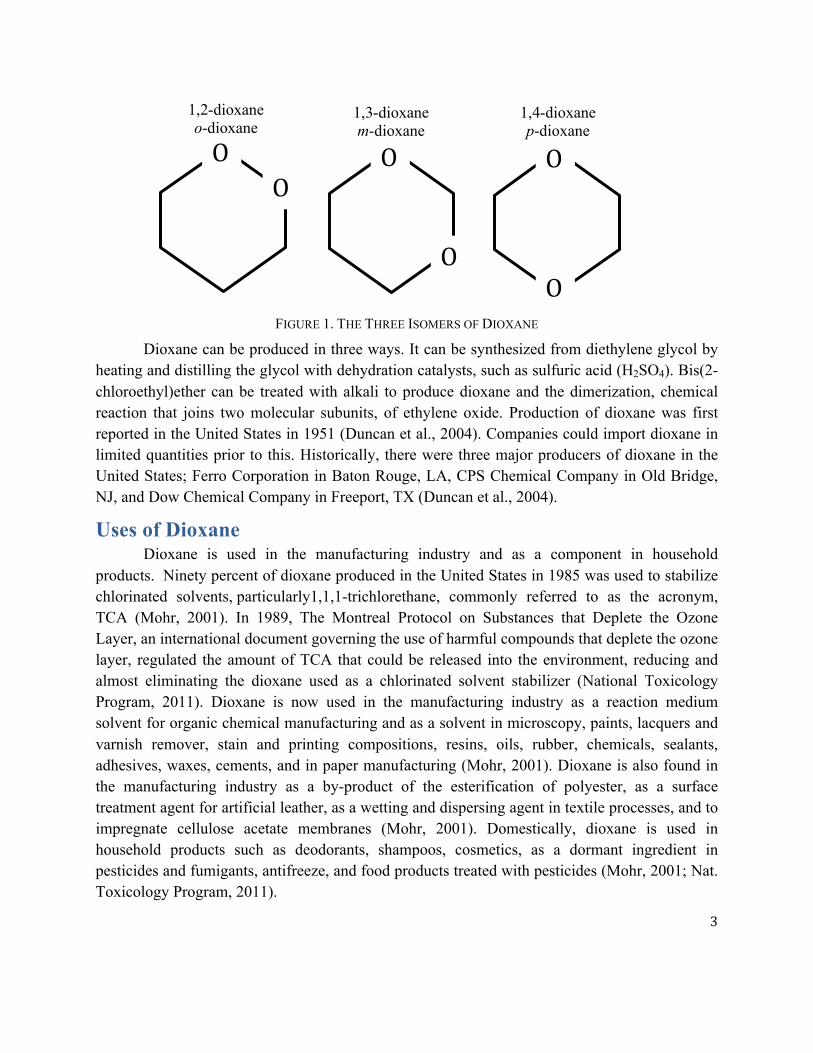
The technical name of 1,4-dioxane distinguishes it from other variations of dioxane. The organic isomers 1,2 and 1,3-dioxane are rare but do exist. Though 1,2 and 1,3-dioxane are related to 1,4-dioxane, their chemical structures, as seen in Figure 1, and uses differ from those of 1,4-dioxane. Because of this, 1,4-dioxane is more commonly referred to simply as dioxane, and will be referred to in all upcoming sections as dioxane. Dioxane is also occasionally referred to as dioxan, p-dioxane, diethylene dioxide, diethylene oxide, diethylene ether, and glycol ethylene ether (Mohr, 2001).

3      

 

 FIGURE 1. THE THREE ISOMERS OF DIOXANE

Dioxane can be produced in three ways. It can be synthesized from diethylene glycol by heating and distilling the glycol with dehydration catalysts, such as sulfuric acid (H2SO4). Bis(2-chloroethyl)ether can be treated with alkali to produce dioxane and the dimerization, chemical reaction that joins two molecular subunits, of ethylene oxide. Production of dioxane was first reported in the United States in 1951 (Duncan et al., 2004). Companies could import dioxane in limited quantities prior to this. Historically, there were three major producers of dioxane in the United States; Ferro Corporation in Baton Rouge, LA, CPS Chemical Company in Old Bridge, NJ, and Dow Chemical Company in Freeport, TX (Duncan et al., 2004).

Uses of Dioxane Dioxane is used in the manufacturing industry and as a component in household

products. Ninety percent of dioxane produced in the United States in 1985 was used to stabilize chlorinated solvents, particularly1,1,1-trichlorethane, commonly referred to as the acronym, TCA (Mohr, 2001). In 1989, The Montreal Protocol on Substances that Deplete the Ozone Layer, an international document governing the use of harmful compounds that deplete the ozone layer, regulated the amount of TCA that could be released into the environment, reducing and almost eliminating the dioxane used as a chlorinated solvent stabilizer (National Toxicology Program, 2011). Dioxane is now used in the manufacturing industry as a reaction medium solvent for organic chemical manufacturing and as a solvent in microscopy, paints, lacquers and varnish remover, stain and printing compositions, resins, oils, rubber, chemicals, sealants, adhesives, waxes, cements, and in paper manufacturing (Mohr, 2001). Dioxane is also found in the manufacturing industry as a by-product of the esterification of polyester, as a surface treatment agent for artificial leather, as a wetting and dispersing agent in textile processes, and to impregnate cellulose acetate membranes (Mohr, 2001). Domestically, dioxane is used in household products such as deodorants, shampoos, cosmetics, as a dormant ingredient in pesticides and fumigants, antifreeze, and food products treated with pesticides (Mohr, 2001; Nat. Toxicology Program, 2011).

O

O

O

O

O

O

1,2-dioxane o-dioxane

1,3-dioxane m-dioxane

1,4-dioxane p-dioxane

4      

 

Dangers of Dioxane Short-term or long-term exposure, each carrying a different set of acute or chronic health

effects can classify human health risks. Acute health effects are identified by sudden and severe exposure and rapid adsorption of the substance. Chronic health effects are identified by prolonged or repeated exposures over many days, months, or years. Acute, exposures to dioxane generally affect the skin and eyes and chronic, exposure affects the liver, kidneys, lungs, skin, brain and eyes. Additional hazards include, a greater risk for pregnant women and flammability caused when dioxane produces explosive peroxides.

Health Hazards This section addresses both short- and long-term exposure of dioxane. Short-term

exposure to low levels of dioxane can cause eye and nose irritation (EPA, 1995). Exposure to very high levels may cause severe kidney and liver effects, vertigo, irritation of the skin, eyes and respiratory passages, nausea, vomiting, and possibly death. (EPA, 1995; EPA, 2000; World Health Organization, 2005). As dioxane vapor is undetectable, acute exposure to high levels has the ability to cause serious injuries to the liver and kidneys without forewarning and illness can become apparent long after exposure (EPA, 1995). Long-term dioxane exposure has not proven to be harmful to humans. However, rats chronically exposed to dioxane have shown liver and kidney damage (Calabrese and Kenyon, 1991).

Carcinogenicity Sufficient evidence shows the carcinogenicity of dioxane in experimental animals.

Carcinogenicity testing has shown that high-dose dioxane can produce hepatocellular carcinomas (cancer of the liver), or adenomas (a benign tumor of epithelial tissue) of the liver and squamous cell carcinomas (skin cancer) of the nasal passages of certain animals. Therefore, the EPA and the IARC have classified dioxane as a Group B2, probable human carcinogen (EPA IRIS 2005; International Agency for Research on Cancer, 1999). It has a carcinogenic oral slope factor, defined by the Technical Education Research Center (TERC) as the percent increase in the risk of getting cancer associated with a dose of the toxin, of 1.1x10-2 milligrams/kilogram/day and its toxicity is currently being reassessed under the EPA Integrated Risk Information System (IRIS) (EPA IRIS 2005; International Agency for Research on Cancer, 1999).

The EPA estimates that, if an individual were to continuously drink water that contained dioxane at an average of 3.0 µg/L over his or her entire lifetime, that person would theoretically have no more than a 1:1,000,000 increased chance of developing cancer. Similarly, the EPA also estimates that drinking water containing 30.0 µg/L would result in not greater than a 1:100,000 chance of developing cancer, and water containing 300.0 µg/L would result in not greater than a 1:10,000 increased chance of developing cancer (Environmental, 2000)

5      

 

Other Dioxane’s other health hazards will not be researched or discussed in this paper though

there are a few other potential risks dioxane poses. Dioxane is known to be a flammable liquid. A well-documented factory explosion at a confectionery research facility in Yokohama, Japan occurred in 1969. Two employees were injured when a drum of dioxane overheated or collided with another drum, sparking the explosion. By the 1970’s, the United States had a workplace air exposure limit of “100 parts of dioxane per million parts (ppm) of air averaged over an eight-hour work shift” (Yoshinaga, 1995). This legislation was intended to prevent inhalation of dioxane in the air by workers as well as spontaneous explosions due to dioxane leaks. Dioxane has also been examined as a risk to pregnant women and prenatal development. A 2007 report compiled information examining the dangers dioxane to infants and reproductive health. The information concluded that a group of chemicals including dioxane elevated the number of miscarriages and stillbirths. The specific role and danger of dioxane is still unknown (Agency for Toxic Substances and Disease Registry, 2012).

Human Exposure Methods of Exposure

Exposure to dioxane occurs through inhalation, dermal contact, or consumption (U.S. EPA, 2013c). Due to a short half-life, dioxane does not remain in the air for a prolonged period of time but contaminated air can be found at sites shortly after a spill or leak. Once a person inhales contaminated air, the lungs rapidly adsorb dioxane into the body (U.S. EPA, 2013c).

Dermal contact with dioxane can occur in a number of ways. Workers can be exposed at a manufacturing job site. Homeowners with contaminated water can encounter dioxane while doing laundry, taking a shower, or while applying cosmetic products, detergents, or shampoos containing dioxane. A survey in the 1990’s found that adult cosmetic products contained, on average, 2-23 ppm of dioxane and children’s cosmetics contained 1.2-12 ppm of dioxane (U.S. EPA, 2013c).

All routes of administration absorb dioxane (HSDB, 1995). In humans, the major metabolite of dioxane is β-hydroxyethoxy acetic acid (HEAA) and the most probable route of excretion is through the kidneys (Young et al., 1976). The enzyme or enzymes responsible for HEAA formation have not been studied, but data from Young et al. (1977) indicates saturation does not occur below an inhalation exposure of 50 ppm for six hours. Although physiologically based pharmacokinetic modeling suggests HEAA is the ultimate toxicant in rodents exposed to dioxane by ingestion, the same modeling procedure does not permit such a distinction for humans exposed by inhalation (Reitz et al., 1990).

6      

 

Case Studies Several studies between 1932 and today have assessed the health effects of dioxane.

These studies have shown enlarged livers and hemorrhagic conditions of the kidneys, abnormal liver function, and death among those exposed. These four studies have indicated the association between dioxane and health risks but they do not indicate a direct correlation.

A German study evaluated the adverse health effects of 74 workers exposed to dioxane in a dioxane-manufacturing plant (Thiess et al., 1977). Each worker had an average potential exposure duration of 25 years at concentrations between 0.01 and 13 ppm. Through clinical evaluations, Thiess evaluated biochemistry parameters of 24 workers who were currently employed in dioxane production, 23 previously exposed workers who still worked in the company and 27 retired or deceased workers. Evidence of abnormal aspartate transaminase (an enzyme found in the blood), alanine transaminase (an enzyme associated with liver function), alkaline phosphatase (an enzyme responsible for removing phosphate groups from molecules), and γ-glutamyl transferase activities (a liver dysfunction indicator) was noted in these workers, but not in those who had retired. The indicators of liver dysfunction, however, could not be separated from alcohol consumption or exposure to ethylene chlorohydrin and/or dichloroethane (Thiess et al., 1977).

A follow-up mortality study was conducted on 165 chemical plant manufacturing and processing workers who were exposed to dioxane levels ranging from less than 25 to greater than 75 ppm between 1954 and 1975 (Buffler et al., 1978). Total deaths due to all causes, including cancer, did not differ from the statewide control group, but the data were not reanalyzed after removing the deaths due to malignant neoplasms. The study is limited by the small number of deaths and by the small sample number. The study did not assess hematologic or clinical parameters that could indicate adverse health effects in the absence of mortality. Though these studies did not show any correlation between increased mortality due to cancer and dioxane exposure, it did not disprove the association between dioxane and cancer.

In 1932, five workers in England died from high exposure to dioxane in an artificial silk plant. The process in the machinery was altered and the vessel containing dioxane lacked exhaust ventilation. Liver and kidney damage was not noted originally but the employees remained out of work due to anorexia, nausea, and vomiting. Sixteen more men were exposed due to an alteration in the machine processes. Seven men became sick within two weeks of the exposure and five died within the month. A general examination of the deceased employees showed enlarged livers and hemorrhagic conditions of the kidneys. A later autopsy found that the employees suffered from edematous, or swollen, lungs and brains, in addition to liver and kidney damage (U.S. Department of Health, Education and Welfare, 1977).

A fatal case of a worker exposed to dioxane for only one week and whose autopsy showed kidney and liver alterations similar to those (Johnstone, 1959). The room in which the patient had worked had no exhaust ventilation and the worker was not provided a respiratory

7      

 

mask. The minimum concentration of dioxane in the room was 208 ppm and the maximum was in excess of 650 ppm with an average concentration of 470 ppm (ATSDR, 2012). Short–term volunteer studies showed that participants who were exposed to high levels of dioxane for a short time experienced symptoms such as mucous irritation in the eyes, nose, and throat (World Health Organization, 2005).

Dioxane in Water Path of Pollution

Dioxane is released into the air, water, and soil in locations that produce or use dioxane (Toxicological Profile 1,4-Dioxane, 2013). Dioxane can evaporate from dry soil to air but the compounds in air rapidly breakdown the dioxane resulting in a 6 to 8 hour half-life. Dioxane that does not evaporate into the air enters the groundwater through the soil. In soil, dioxane can rapidly diffuse through low permeability soils, such as silts and clays, allowing it to enter and fully dissolve in to a groundwater source (Report on Carcinogens, Twelfth Edition 2011). Due to

its low Henry’s Law constant (4.80x10-6 !"#  !"!

!"#) dioxane cannot volatize once it has entered a

water source (Report on Carcinogens, Twelfth Edition 2011). The Henry’s Law constant is the air-water distribution ratio, which is the ratio of a compound’s abundance in the gas phase to that in the aqueous phase at equilibrium. Henry’s Law constant shows that once in water, dioxane is stable and unwilling to evaporate to a gas phase.

Dioxane is weakly affected by adsorption, thus allowing it to easily travel through the water source. The concentration of dioxane in the groundwater source will not undergo biodegradation and will remain relatively constant through transportation (Report on Carcinogens, Twelfth Edition 2011). These physical and chemical properties allow dioxane plumes to measure twice the length of similar solvent plumes and effect areas up to six times larger. Therefore, remediating a dioxane plume in a groundwater source is significantly more difficult than other chlorinated solvent plumes (Walsom and Tunnicliffe, 2002).

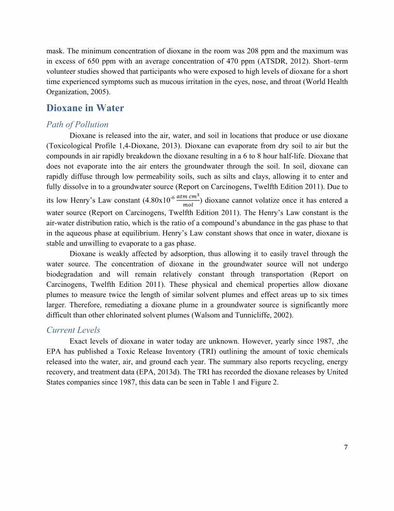
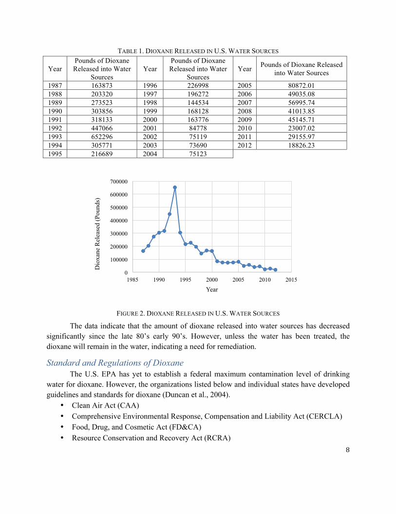
Current Levels Exact levels of dioxane in water today are unknown. However, yearly since 1987, ,the

EPA has published a Toxic Release Inventory (TRI) outlining the amount of toxic chemicals released into the water, air, and ground each year. The summary also reports recycling, energy recovery, and treatment data (EPA, 2013d). The TRI has recorded the dioxane releases by United States companies since 1987, this data can be seen in Table 1 and Figure 2.

8      

 

TABLE 1. DIOXANE RELEASED IN U.S. WATER SOURCES

Year Pounds of Dioxane Released into Water

Sources Year

Pounds of Dioxane Released into Water

Sources Year Pounds of Dioxane Released

into Water Sources

1987 163873 1996 226998 2005 80872.01 1988 203320 1997 196272 2006 49035.08 1989 273523 1998 144534 2007 56995.74 1990 303856 1999 168128 2008 41013.85 1991 318133 2000 163776 2009 45145.71 1992 447066 2001 84778 2010 23007.02 1993 652296 2002 75119 2011 29155.97 1994 305771 2003 73690 2012 18826.23 1995 216689 2004 75123

 

FIGURE 2. DIOXANE RELEASED IN U.S. WATER SOURCES

The data indicate that the amount of dioxane released into water sources has decreased significantly since the late 80’s early 90’s. However, unless the water has been treated, the dioxane will remain in the water, indicating a need for remediation.

Standard and Regulations of Dioxane The U.S. EPA has yet to establish a federal maximum contamination level of drinking water for dioxane. However, the organizations listed below and individual states have developed guidelines and standards for dioxane (Duncan et al., 2004).

• Clean Air Act (CAA) • Comprehensive Environmental Response, Compensation and Liability Act (CERCLA) • Food, Drug, and Cosmetic Act (FD&CA) • Resource Conservation and Recovery Act (RCRA)

0

100000

200000

300000

400000

500000

600000

700000

1985 1990 1995 2000 2005 2010 2015

Dio

xane

Rel

ease

d (P

ound

s)

Year

9      

 

• Superfund Amendments and Reauthorization Act (SARA) • The Occupational Safety and Health Administration (OSHA) • American Conference of Governmental Industrial Hygienists (ACGIH)

The CAA has listed dioxane as a hazardous air pollutant. CERCLA has established 100 pounds as the reportable quantity standard for emissions. The FD&CA set 10 ppm as the limit of dioxane in glycerides and polyglycerides of hydrogenated vegetable oils when used as a food additive. RCRA require all companies to report and record any dioxane waste produced. SARA has set general threshold amounts for production and usage within a facility. OSHA set the average 8-hour time-weighted average airborne permissible exposure limit at 360 mg/m3 or 100 mg/L. The ACGIH set a dermal threshold value limit of 25 mg/L and recommends an airborne exposure limit of 20 mg/L averaged over an 8-hour time-weight average. The NIOSH set 500 mg/L as the concentration that is immediately dangerous to life or health and recommends an airborne exposure limit of 1 mg/L.

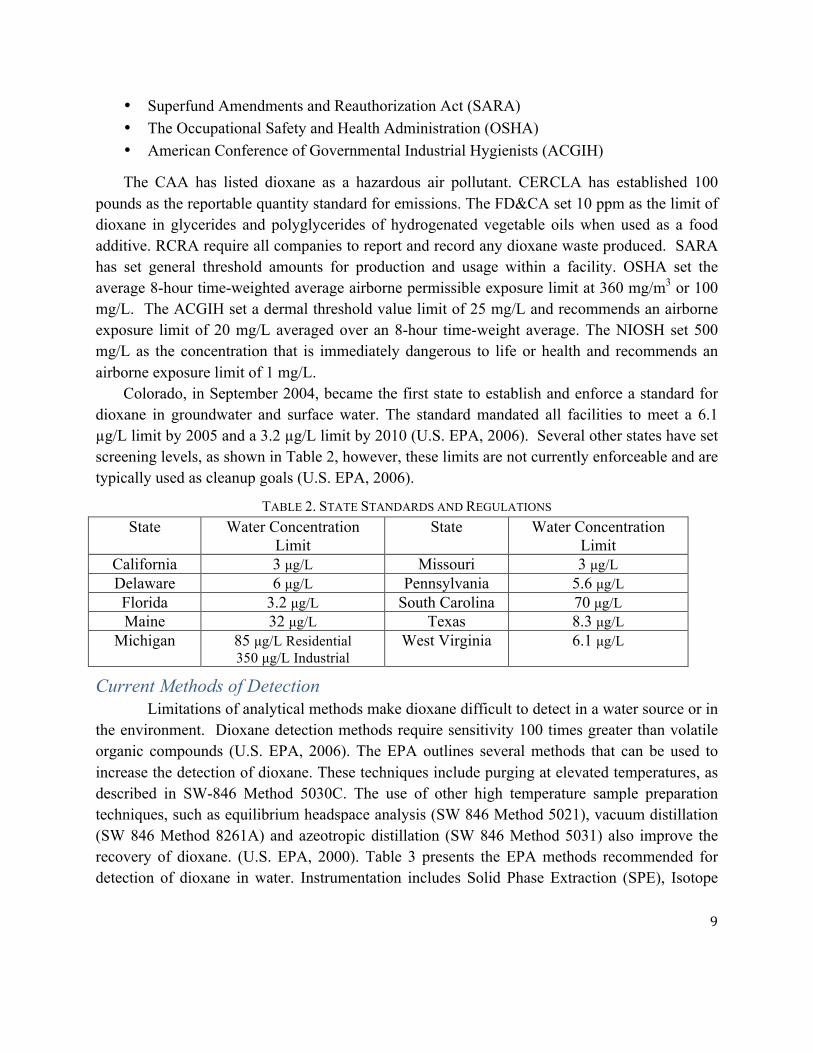
Colorado, in September 2004, became the first state to establish and enforce a standard for dioxane in groundwater and surface water. The standard mandated all facilities to meet a 6.1 µg/L limit by 2005 and a 3.2 µg/L limit by 2010 (U.S. EPA, 2006). Several other states have set screening levels, as shown in Table 2, however, these limits are not currently enforceable and are typically used as cleanup goals (U.S. EPA, 2006).

TABLE 2. STATE STANDARDS AND REGULATIONS State Water Concentration

Limit State Water Concentration

Limit California 3 µg/L Missouri 3 µg/L Delaware 6 µg/L Pennsylvania 5.6 µg/L Florida 3.2 µg/L South Carolina 70 µg/L Maine 32 µg/L Texas 8.3 µg/L

Michigan 85 µg/L Residential 350 µg/L Industrial

West Virginia 6.1 µg/L

Current Methods of Detection Limitations of analytical methods make dioxane difficult to detect in a water source or in

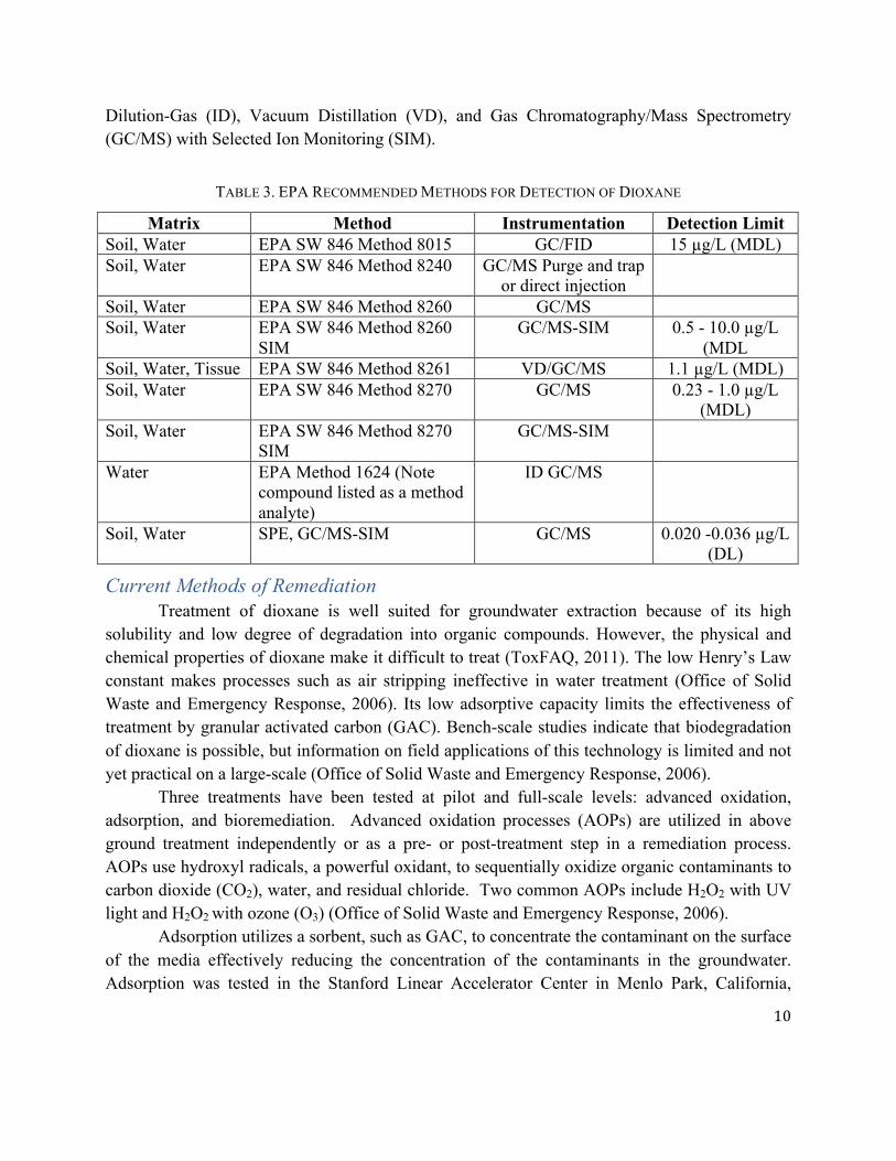
the environment. Dioxane detection methods require sensitivity 100 times greater than volatile organic compounds (U.S. EPA, 2006). The EPA outlines several methods that can be used to increase the detection of dioxane. These techniques include purging at elevated temperatures, as described in SW-846 Method 5030C. The use of other high temperature sample preparation techniques, such as equilibrium headspace analysis (SW 846 Method 5021), vacuum distillation (SW 846 Method 8261A) and azeotropic distillation (SW 846 Method 5031) also improve the recovery of dioxane. (U.S. EPA, 2000). Table 3 presents the EPA methods recommended for detection of dioxane in water. Instrumentation includes Solid Phase Extraction (SPE), Isotope

10      

 

Dilution-Gas (ID), Vacuum Distillation (VD), and Gas Chromatography/Mass Spectrometry (GC/MS) with Selected Ion Monitoring (SIM).

TABLE 3. EPA RECOMMENDED METHODS FOR DETECTION OF DIOXANE

Matrix Method Instrumentation Detection Limit Soil, Water EPA SW 846 Method 8015 GC/FID 15 µg/L (MDL) Soil, Water EPA SW 846 Method 8240 GC/MS Purge and trap

or direct injection

Soil, Water EPA SW 846 Method 8260 GC/MS Soil, Water EPA SW 846 Method 8260

SIM GC/MS-SIM 0.5 - 10.0 µg/L

(MDL Soil, Water, Tissue EPA SW 846 Method 8261 VD/GC/MS 1.1 µg/L (MDL) Soil, Water EPA SW 846 Method 8270 GC/MS 0.23 - 1.0 µg/L

(MDL) Soil, Water EPA SW 846 Method 8270

SIM GC/MS-SIM

Water EPA Method 1624 (Note compound listed as a method analyte)

ID GC/MS

Soil, Water SPE, GC/MS-SIM GC/MS 0.020 -0.036 µg/L (DL)

Current Methods of Remediation Treatment of dioxane is well suited for groundwater extraction because of its high

solubility and low degree of degradation into organic compounds. However, the physical and chemical properties of dioxane make it difficult to treat (ToxFAQ, 2011). The low Henry’s Law constant makes processes such as air stripping ineffective in water treatment (Office of Solid Waste and Emergency Response, 2006). Its low adsorptive capacity limits the effectiveness of treatment by granular activated carbon (GAC). Bench-scale studies indicate that biodegradation of dioxane is possible, but information on field applications of this technology is limited and not yet practical on a large-scale (Office of Solid Waste and Emergency Response, 2006).

Three treatments have been tested at pilot and full-scale levels: advanced oxidation, adsorption, and bioremediation. Advanced oxidation processes (AOPs) are utilized in above ground treatment independently or as a pre- or post-treatment step in a remediation process. AOPs use hydroxyl radicals, a powerful oxidant, to sequentially oxidize organic contaminants to carbon dioxide (CO2), water, and residual chloride. Two common AOPs include H2O2 with UV light and H2O2 with ozone (O3) (Office of Solid Waste and Emergency Response, 2006).

Adsorption utilizes a sorbent, such as GAC, to concentrate the contaminant on the surface of the media effectively reducing the concentration of the contaminants in the groundwater. Adsorption was tested in the Stanford Linear Accelerator Center in Menlo Park, California,

11      

 

where dioxane originally detected at concentrations up to 7,300 µg/L was reduced below detection level (Office of Solid Waste and Emergency Response, 2006).

Bioremediation places contaminated water in contact with microorganisms in attached or suspended growth bioreactors to allow the microorganisms to metabolize the dioxane. A pilot study was conducted using Kaldnes, a buoyant plastic media, in a fixed-film biological process to treat dioxane in a groundwater source. The pilot scale system reduced the initial concentration of the dioxane (8,000 µg/L – 12,000 µg/L) to concentrations less than 200 µg/L (Office of Solid Waste and Emergency Response, 2006).

UV and Hydrogen Peroxide Ultraviolet Degradation

Recent increases in regulations concerning drinking water quality have accelerated the use of UV technology in the United States. A UV degradation system preforms radiation, photolysis, or oxidation within a system. UV degradation is commonly used with other treatment methods to enhance the rate of degradation (Pereira et al., 2007).

UV treatment lamps are produced at both low- and medium- pressure. The conventional lamp used in UV treatment is a low-pressure mercury lamp that emits UV light at 253.7 nm. This lamp is commonly used for the degradation of microorganisms within a waste or drinking water treatment plant. The secondary lamp also used in UV treatment is a medium-pressure polychromatic mercury lamp that emits light between 205 and 500 nm. Batch scale tests have shown that medium-pressure lamps have been effective in oxidizing various organic compounds.

UV treatment can causes photolysis within the sample being treated. Photolysis occurs when a chemical species adsorbs photons and undergoes a chemical change. Photolysis occurs at UV wavelengths lower than 300nm (Avisar et al., 2010). UV treatment has be ability to disassociate compounds in water; however, it does not degrade the disassociated compounds.

UV/ H2O2 Advanced Oxidation Process The most effective UV treatments were obtained when highly reactive and nonselective

hydroxyl radicals (OH-) are formed during treatment. To form OH- radicals, the addition of photo catalysts such as ozone (O3), titanium dioxide (TiO2), or H2O2 were required (Pereira et al., 2007). The oxidation strength of OH- radicals produced with the addition of H2O2 is much greater than other agents such as ozone and chlorine making it more capable of oxidizing an assortment of organic and inorganic contaminants (IJpelaar, 2007). The process is completed when the UV light catalyzes the dissociation of H2O2 in the OH- radicals through chain reactors. The oxidants react with the contaminants in the water and have been proven to destroy organic compounds in ground and surface water (IJpelaar, 2007). Through batch scale treatmens, the addition of H2O2 has been shown to efficiently remove methyl tert-butyl ether from contaminated drinking water, N-nitrosodimethylamine during batch scale modeling of drinking water, and endocrine-disrupting compounds from laboratory grade water (Pereira et al., 2007).

12      

 

Current Application Four full scale UV/ H2O2 treatment processes for dioxane have been implemented at the

following sites: McClellan Air Force Base (AFB) in Sacramento, California; Gloucester Landfill in Ontario, Canada; Charles George Landfill in Tyngsborough, Massachusetts; and the Pall-Gelman Sciences site in Ann Arbor, Michigan.

McClellan AFB installed a UV and H2O2 system initially to treat vinyl chloride contamination on the site. After the vinyl chloride concentrations were reduced to the maximum contamination level, the system was shut down. The discovery of dioxane at the contamination site allowed the full-scale model to be tested on the removal of dioxane. The system was restarted in October of 2003 and has treated approximately 2.7 million gallons of water per month. The system has effectively reduced the amount of dioxane below the EPA Region 9 tap water preliminary remediation goal (PRG) of 6.1 µg/L and completed in 2006 (Office of Solid Waste and Emergency Response, 2006).

Groundwater at the Gloucester Landfill in Ontario, Canada is treated with an AOP utilizing UV and H2O2 treatment. From 1969 to 1980 this site was used as a disposal area for a federal laboratory, university, and hospital wastes. The chemicals present in the wastes contaminated a shallow, unconfined aquifer and a deep confined aquifer below the site. In 1992, a 29 well pump and treat system was put into operation on the site to treat 132 gallons per minute (gpm) from the deep aquifer and 61 gpm from the shallow aquifer. The treatment process included a dose of acid to reduce the pH into operating range for treatment, a series of UV lamps with doses of H2O2 through the system and a final step to readjust the pH. The treated water was reinjected into the aquifers at five locations upgradient of the contamination site (Office of Solid Waste and Emergency Response, 2006).

The Charles George Landfill Superfund site in Tyngsborough, Massachusetts utilized UV/ H2O2 to treat 3.6 million gallons of contaminated water pumped to a storage lagoon. The system treated dioxane to a concentration of 7 µg/L to meet the water discharge specified by the Superfund record of decision (Office of Solid Waste and Emergency Response, 2006).

A company unintentionally released dioxane to the Pall-Gelman Sciences site during the manufacturing of micro porous filters from the 1960s to 1980s. Wastewater from the company was released into a treatment pond where groundwater samples collected measured concentrations as high as 221,000 µg/L. Dioxane contaminated aquifers up to two miles from the source of the contamination in multiple plumes. After treatment with UV and H2O2 concentrations of effluent water ranged from nondetect to 10 µg/L. Since 1997, more than two billion gallons of groundwater has been treated and discharged, and removed more than 60,000 pounds of dioxane from the contaminated water (Office of Solid Waste and Emergency Response, 2006).

Analytic Analysis To enhance the knowledge and refine standards of dioxane, there is a need for

epidemiological studies that show the correlation between health risks and dioxane contamination. These studies can be conducted using an analytical approach to epidemiology.

13      

 

Statistics is characterized by the practice or science of collecting and analyzing numerical data in large quantities, with a focus on inferring proportions in a whole from those in a representative sample. Statistics have been used since the late 16th century to make inferences about the state of complex systems (Stephenson, 2000). However, in the past two decades, analytics has become an emerging analysis technique to deliver, collect, and use whole data sets to generate insights that inform fact-based decisions. It consists of four phases: preparation, preprocessing, analysis and post-processing. During preparation, a plan for the collection of data is made, the data is collected and the appropriate data sets are identified. Preprocessing cleans, filters, standardizes, and collects missing data. Analysis includes classifying data, determining correlations and regressions in the data, forecasting future trends, and providing correlations of the past. Post processing is interpreting, evaluating and documenting the organized data (Runkler, 2012). Analytics can be classified as descriptive or predictive. Descriptive analytics provides a representation of the knowledge discovered from historic data. Descriptive aims to predict future events, while predictive analytics aims to analyze a data set for determining the probability that some scenario is likely to happen (Matlis, 2006). Analytics is being used in many different fields including healthcare, sports, business, and epidemiology. For example, a study of all patients admitted to the National Paraplegic Center of Toledo for spinal cord injuries, during a six-month period were analyzed for potential clinical urinary tract infections (Herruzo et al., 1994). The predictive analytical study determined risk factors, age, hospitalization period and spinal cord injury that could lead to a clinical urinary tract infection. A mathematical equation was established to predict clinical urinary tract infections when a patient was admitted to the center.

 

14      

 

Methodology Experimental Methodology

The primary goal of this project was to determine whether UV and H2O2 would effectively reduce the amount of dioxane in a water source. A series of experiments exposed dioxane to H2O2, UV, and H2O2/UV over different times and pH levels. The amount of dioxane in the water source was quantified using an Agilent Technologies 6890N GC system. Stock Solutions Three stock solutions of known initial concentrations were created for all experiments. A 200 mL 5 mg/L dioxane stock solution was prepared weekly using reagent grade water (ROpure ST Reverse Osmosis/tank system) and pure dioxane. The pure dioxane was diluted in two steps: first 50 µL of dioxane were added to 100 mL of reagent grade water and mixed for 24 hours. Next, 1.94 mL of the solution were added to a 200 mL amber bottle with 200 mL of reagent grade water and mixed for another 24 hours to achieve the desired concentration. A 0.29 g/L H2O2 stock solution was prepared using 30 percent H2O2 and reagent grade water. The H2O2

solution was prepared once during the term by adding 167 µL of 30 percent H2O2 and 250 mL of reagent grade water to an amber vial and mixed for 30 minutes. The solution was mixed for 1 minute before every use. A 250 mg/L chlorobenzene stock solution was prepared weekly using pure chlorobenzene and reagent grade water. The pure chlorobenzene was diluted in two steps. First, 61 µL of aqueous chlorobenzene was added to 250 mL of reagent grade water and mixed for 24 hours. Next, 1 mL of the mixed solution was added to an 25 mL amber vial with 24 mL of lab water to achieve a concentration of 250 mg/L.

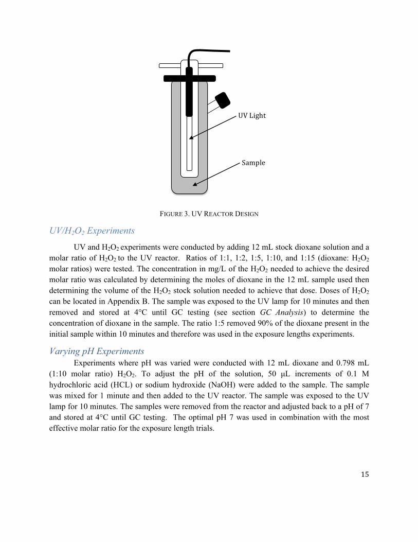
Ultraviolet Degradation UV lab scale batch reactor tests were conducted in an ACE Glass 7880 reaction assembly,

photochemical, microscale (#25, 14,10) reactor (Figure 3). The reactor consists of a quartz center tube surrounded by a glass encasement that holds 12 mL. Each experiment was conducted with a Pen-Ray 5.5 watt Lamp (ACE No. 12132-08). The Pen-Ray Lamp is a low pressure UV lamp with an output at 254 nm. The lamp is made of double bore quartz, creating an arc of UV when the plasma ignites at one electrode and continues around the septum and back to the other electrode. Initial experiments tested various molar ratios of H2O2 added to the sample before UV treatment. pH test were conducted at values of 4, 7, and 9 to determine an optimal pH for kinetic trials. Finally, the most efficient ratio was used to test the kinetics of the dioxane degradation at 30 seconds, 1, 2, 4, 6, 10, 12, and 15 minutes.

15      

 

 

FIGURE 3. UV REACTOR DESIGN

UV/H2O2 Experiments

UV and H2O2 experiments were conducted by adding 12 mL stock dioxane solution and a molar ratio of H2O2 to the UV reactor. Ratios of 1:1, 1:2, 1:5, 1:10, and 1:15 (dioxane: H2O2 molar ratios) were tested. The concentration in mg/L of the H2O2 needed to achieve the desired molar ratio was calculated by determining the moles of dioxane in the 12 mL sample used then determining the volume of the H2O2 stock solution needed to achieve that dose. Doses of H2O2 can be located in Appendix B. The sample was exposed to the UV lamp for 10 minutes and then removed and stored at 4°C until GC testing (see section GC Analysis) to determine the concentration of dioxane in the sample. The ratio 1:5 removed 90% of the dioxane present in the initial sample within 10 minutes and therefore was used in the exposure lengths experiments.

Varying pH Experiments Experiments where pH was varied were conducted with 12 mL dioxane and 0.798 mL (1:10 molar ratio) H2O2. To adjust the pH of the solution, 50 µL increments of 0.1 M hydrochloric acid (HCL) or sodium hydroxide (NaOH) were added to the sample. The sample was mixed for 1 minute and then added to the UV reactor. The sample was exposed to the UV lamp for 10 minutes. The samples were removed from the reactor and adjusted back to a pH of 7 and stored at 4°C until GC testing. The optimal pH 7 was used in combination with the most effective molar ratio for the exposure length trials.

Sample  

UV  Light  

16      

 

Exposure Length Experiments To test the kinetics of the UV/H2O2 treatment, and the degradation of the dioxane during the UV experiment, exposure length experiments were conducted. Twelve milliliters of dioxane stock solution and 0.399 mL (1:5 molar ratio) of H2O2 stock solution were mixed for 30 seconds and then added to the UV reactor. The sample was exposed to the UV lamp for reaction times of 30 seconds, 1, 2, 4, 6, 10, and 15 minutes. Eighty microliters of pure methanol was added to the sample and the dioxane was quantified using GC analysis.

Controls A control group of samples were tested to use as a baseline for the experiments. A

sample of stock dioxane solution tested the initial concentration of dioxane in the samples. A sample of dioxane with the molar ratio 1:5 and no UV treatment tested the effectiveness of H2O2

without UV photolysis. A sample of dioxane exposed to the UV lamp with no H2O2 tested the success of UV photolysis on degrading dioxane independently. A sample of stock dioxane solution transferred from the UV reactor, to the storage vials, and then to GC vials tested the amount of dioxane lost during transfers. A blank reagent grade water sample tested the amount of dioxane in the reagent grade water.

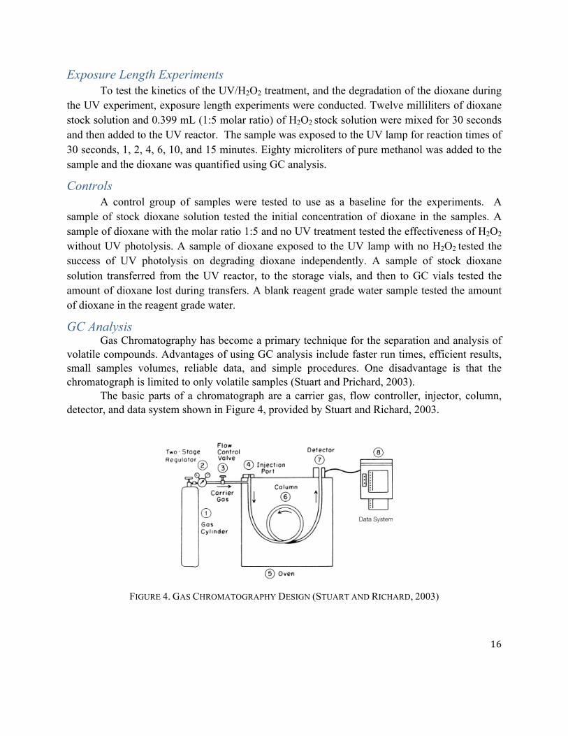
GC Analysis Gas Chromatography has become a primary technique for the separation and analysis of volatile compounds. Advantages of using GC analysis include faster run times, efficient results, small samples volumes, reliable data, and simple procedures. One disadvantage is that the chromatograph is limited to only volatile samples (Stuart and Prichard, 2003). The basic parts of a chromatograph are a carrier gas, flow controller, injector, column, detector, and data system shown in Figure 4, provided by Stuart and Richard, 2003.

 

FIGURE 4. GAS CHROMATOGRAPHY DESIGN (STUART AND RICHARD, 2003)

17      

 

The GC runs as follows: an inert carrier gas flows continuously from a gas cylinder through the injection port, the column, and the detector. The sample is injected into the heated injected inlet, vaporized and then carried into the column. The sample divides between the mobile and stationary phases and then separates into components based on solubility in the liquid phase and vapor pressure. After passing through the column, the carrier gas and sample pass through a detector where the GC measures the quantity of the sample and generates an electrical signal. This signal then goes to the data system where a chromatogram, a display of the data calculated by the GC, is generated (Stuart and Prichard, 2003). The GC analysis was conducted on an Agilent Technologies 6890N GC system. Ten milliliters of a sample, 4 g of sodium chloride NaCl and 50 µL of 250 mg/L chlorobenzene were added to a GC test vial. The test vials were loaded into the GC and programmed into the computer. Once the machine ran the sample, the chromatogram for each sample was printed. The area of the spike was internally calculated and compared to a standard curve found in Appendix C. The standard curve were used to solve for the concentration of dioxane in the sample.

Analytic  Methodology  The analytical approach was broken into two separate studies. The first study examined

the occurrence of associated chronic illnesses (kidney and liver cancer) to the location of dioxane contamination sites. The second study compared various social metrics, such as poverty rate and median household income, of the municipalities containing the contamination sites to the social metrics of the overarching county as a whole.

Contamination sites, listed in Appendix D, were selected from the Toxic Release Inventory (TRI) based upon the following criteria:

• Companies that released a minimum of 100 pounds of dioxane per year • Companies that release dioxane for more than 10 years • Companies that started releasing dioxane prior to 2000

The amount of dioxane released at each contamination site can be seen in Appendix E. Since healthcare treatment, especially for chronic illness, takes place and is reported at a

county level. For comparative purposes, control groups were established. Counties within the same state were examined for comparable populations. Those within five percent of the same population were then compared for population densities. This process ensured that the control was as similar as possible to the test group. Remaining within the state preserved geographic and cultural similarities.

The municipalities used in the initial test were again used as test subjects in the second test. The second test used the overarching counties as comparison, though the county data did include the individual municipality. The data sets between the two were examined for comparison. The differences in social metrics between test and control groups were noted.

18      

 

This study was also expanded to include state and national county data for comparative purposes. Geographic Information Systems (GIS) were implemented to assist in creating comparative displays.

 

19      

 

Results and Discussion The objective of this study was to obtain data for the degradation of dioxane using

UV/H2O2 oxidation at five molar ratios: 1:0, 1:1, 1:5, 1:10 and 1:15 (dioxane to H2O2). The data were analyzed to determine the effectiveness of each ratio and to make recommendations for treatment and future research.

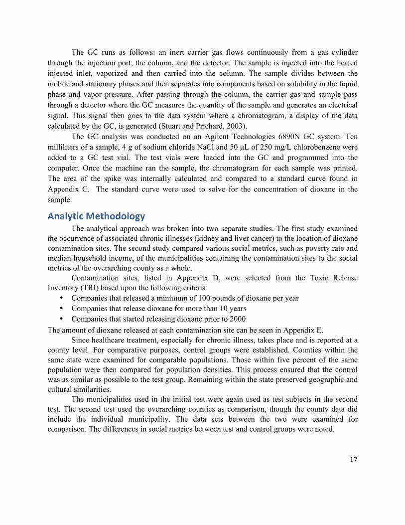
Experimental   All molar ratios removed over 90 percent of the initial dioxane when exposed to the UV light for 30 minutes. Figure 5 presents the residual concentrations of dioxane after a 30 minute exposure time. The initial concentration is indicated by the molar ratio of 1:0.

 

FIGURE 5. MOLAR RATIO OF DIOXANE TO H2O2 30 MINUTE TESTS, INITIAL DIOXANE CONCENTRATION 5 MG/L

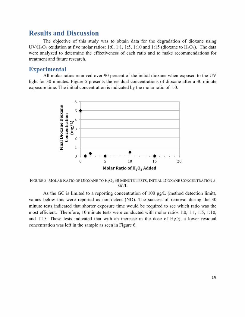
As the GC is limited to a reporting concentration of 100 µg/L (method detection limit), values below this were reported as non-detect (ND). The success of removal during the 30 minute tests indicated that shorter exposure time would be required to see which ratio was the most efficient. Therefore, 10 minute tests were conducted with molar ratios 1:0, 1:1, 1:5, 1:10, and 1:15. These tests indicated that with an increase in the dose of H2O2, a lower residual concentration was left in the sample as seen in Figure 6.

0  

1  

2  

3  

4  

5  

6  

0   5   10   15   20  

Final  Dioxane  Dioxane  

Concentration    

(mg/L)  

Molar  Ratio  of  H2O2  Added  

20      

 

 

FIGURE 6. MOLAR RATIO OF DIOXANE TO H2O2 10 MINUTE TESTS, 5 MG/L INITIAL DIOXANE CONCENTRATION

The efficiency of each dose was calculated to determine the dose that would provide kinetic data. The efficiency of treatment was calculated using Equation 1.

𝐸𝑓𝑓𝑖𝑐𝑖𝑒𝑛𝑐𝑦 = !!!!!!!

×100% (Equation 1)

CI and CF represent the initial and final concentrations at each molar ratio respectively. The efficiency of each dose is summarized in Table 4.

TABLE 4. EFFECTIVENESS OF DIOXANE H2O2 MOLAR RATIO FOR A 10 MINUTES REACTION TIME

Molar Ratio Final

Concentration (mg/L)

Effectiveness%

Initial Concentration 3.83 0 1:0 2.89 25 1:1 1.03 73 1:5 0.3189 92 1:10 ND >97 1:15 ND >97

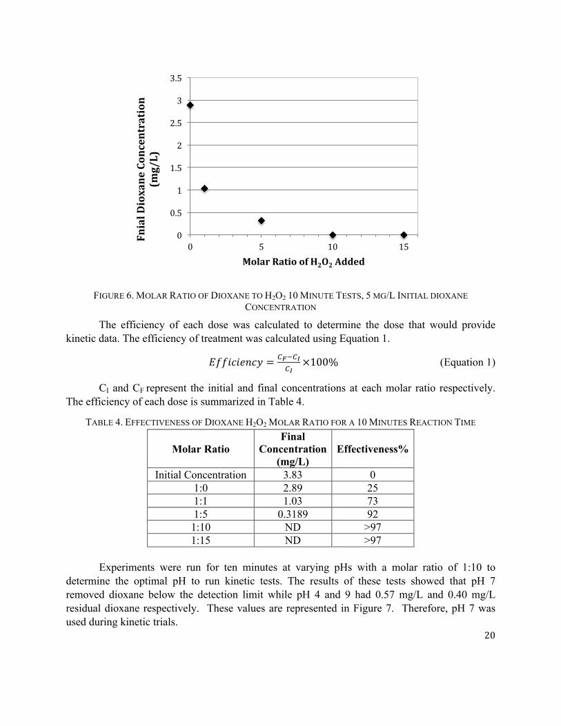
Experiments were run for ten minutes at varying pHs with a molar ratio of 1:10 to

determine the optimal pH to run kinetic tests. The results of these tests showed that pH 7 removed dioxane below the detection limit while pH 4 and 9 had 0.57 mg/L and 0.40 mg/L residual dioxane respectively. These values are represented in Figure 7. Therefore, pH 7 was used during kinetic trials.

0  

0.5  

1  

1.5  

2  

2.5  

3  

3.5  

0   5   10   15  

Fnial  Dioxane  Concentration    

(mg/L)  

Molar  Ratio  of  H2O2  Added    

21      

 

 

FIGURE 7. 10 MINUTE 1:10 RATIO PH TESTS, 3.83 MG/L INITIAL DIOXANE CONCENTRATION

The final concentration with doses of 1:10 and 1:15 were below the detection limit after 10 minutes of UV exposure. Therefore, the ratio of 1:5 was selected for kinetic trials to determine the kinetic constant. The molar ratio of 1:5 was tested at 30 seconds, 1, 2, 4, 6, 10, 12 and 15 minutes. The kinetic data were used to determine the rate constant of degradation. Table 5 summarizes the concentrations of dioxane after each exposure time.

TABLE 5. RESIDUAL DIOXANE CONCENTRATION AFTER VARIOUS EXPOSURE TIMES

Time (min) Residual

Concentration (mg/L)

0 3.57 .5 2.40 1 2.10 2 1.56 4 1.35 6 0.92 10 0.69 12 0.80 15 0.17

This data set was used to determine the rate constant for the first order degradation of dioxane. The rate of degradation was calculated using Equation 2.

𝑅𝑎𝑡𝑒  𝑜𝑓  𝐷𝑒𝑔𝑟𝑎𝑑𝑎𝑡𝑖𝑜𝑛 =     !"!"= −𝑘𝐶 (Equation 2)

0  

0.1  

0.2  

0.3  

0.4  

0.5  

0.6  

4   7   9  

Fina

l Dio

xane

Con

cent

ratio

n (m

g/L

)

pH

22      

 

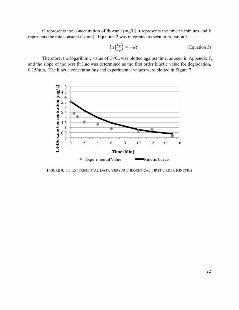
C represents the concentration of dioxane (mg/L), t represents the time in minutes and k represents the rate constant (1/min). Equation 2 was integrated as seen in Equation 3.

ln !!!!

= −𝑘𝑡 (Equation 3)

Therefore, the logarithmic value of Cf/Co was plotted against time, as seen in Appendix F, and the slope of the best fit line was determined as the first order kinetic value for degradation, 0.15/min. The kinetic concentrations and experimental values were plotted in Figure 7.

 

FIGURE 8. 1:5 EXPERIMENTAL DATA VERSUS THEORETICAL FIRST ORDER KINETICS

   

0  0.5  1  

1.5  2  

2.5  3  

3.5  4  

4.5  5  

0   2   4   6   8   10   12   14   16  

1,4-­‐Dioxane  Concentration  (m

g/L)  

Time  (Min)  

Experimental  Value   Kinetic  Curve  

23      

 

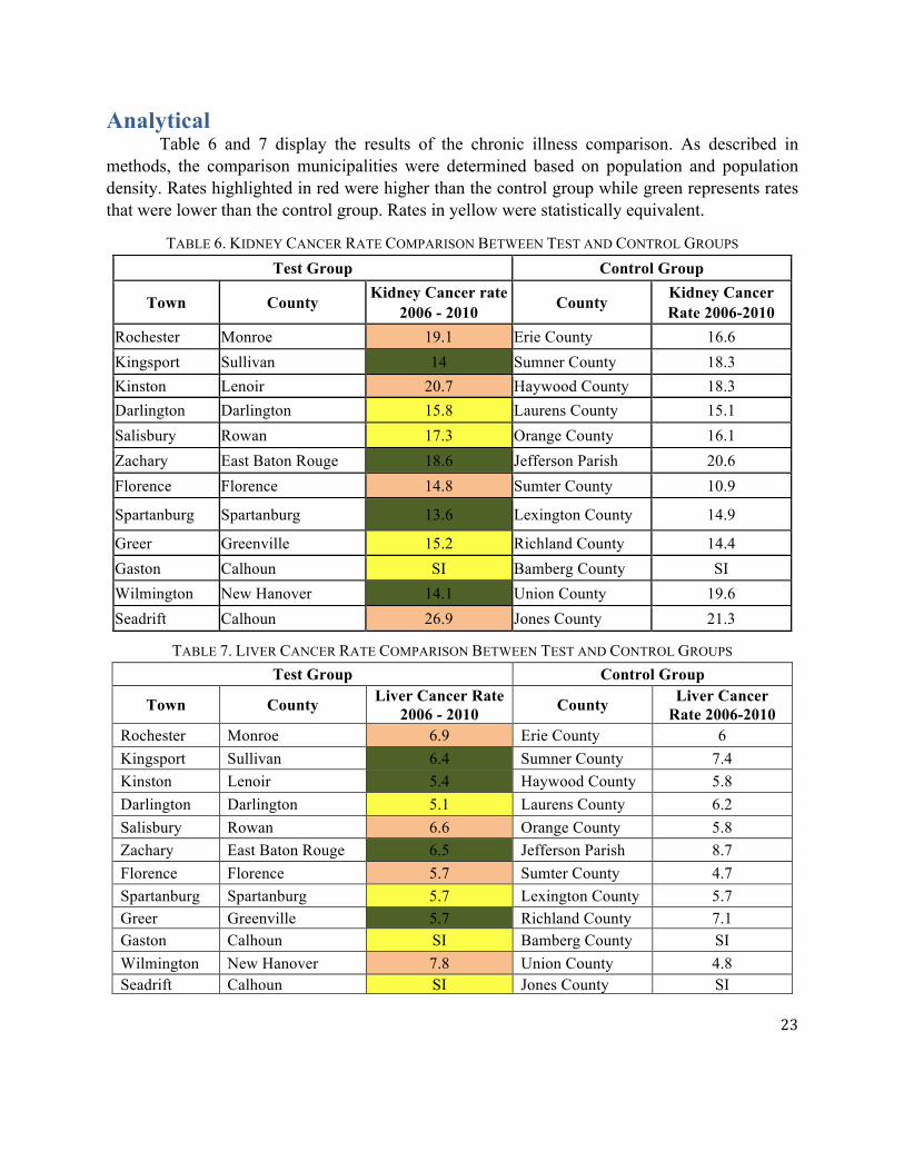
Analytical Table 6 and 7 display the results of the chronic illness comparison. As described in

methods, the comparison municipalities were determined based on population and population density. Rates highlighted in red were higher than the control group while green represents rates that were lower than the control group. Rates in yellow were statistically equivalent.

TABLE 6. KIDNEY CANCER RATE COMPARISON BETWEEN TEST AND CONTROL GROUPS Test Group Control Group

Town County Kidney Cancer rate 2006 - 2010 County Kidney Cancer

Rate 2006-2010 Rochester Monroe 19.1 Erie County 16.6 Kingsport Sullivan 14 Sumner County 18.3 Kinston Lenoir 20.7 Haywood County 18.3 Darlington Darlington 15.8 Laurens County 15.1 Salisbury Rowan 17.3 Orange County 16.1 Zachary East Baton Rouge 18.6 Jefferson Parish 20.6 Florence Florence 14.8 Sumter County 10.9

Spartanburg Spartanburg 13.6 Lexington County 14.9

Greer Greenville 15.2 Richland County 14.4 Gaston Calhoun SI Bamberg County SI Wilmington New Hanover 14.1 Union County 19.6 Seadrift Calhoun 26.9 Jones County 21.3

TABLE 7. LIVER CANCER RATE COMPARISON BETWEEN TEST AND CONTROL GROUPS Test Group Control Group

Town County Liver Cancer Rate 2006 - 2010 County Liver Cancer

Rate 2006-2010 Rochester Monroe 6.9 Erie County 6 Kingsport Sullivan 6.4 Sumner County 7.4 Kinston Lenoir 5.4 Haywood County 5.8 Darlington Darlington 5.1 Laurens County 6.2 Salisbury Rowan 6.6 Orange County 5.8 Zachary East Baton Rouge 6.5 Jefferson Parish 8.7 Florence Florence 5.7 Sumter County 4.7 Spartanburg Spartanburg 5.7 Lexington County 5.7 Greer Greenville 5.7 Richland County 7.1 Gaston Calhoun SI Bamberg County SI Wilmington New Hanover 7.8 Union County 4.8 Seadrift Calhoun SI Jones County SI

24      

 

A brief analysis yields very mixed results, with a slightly more convincing trend present in the liver cancer data. Analytically, this study would have to be declared inconclusive. Despite a number of data points following the predicted trend, there are almost as many points that defy the predicted trend. The abundance of statistically equivalent and statistically inconclusive numbers only further cloud the data as a whole. These discrepancies can be attributed to a vast array of causes, many of which are rooted in the broadness of this study. County data related to a single contamination site includes enormous amounts of excess test subjects. Other factors in the control groups could also alter those numbers, since the control group was only established based on population and population density. While the data may not appear very promising, declaring this study a failure would be equally as premature as declaring an established trend within the data.

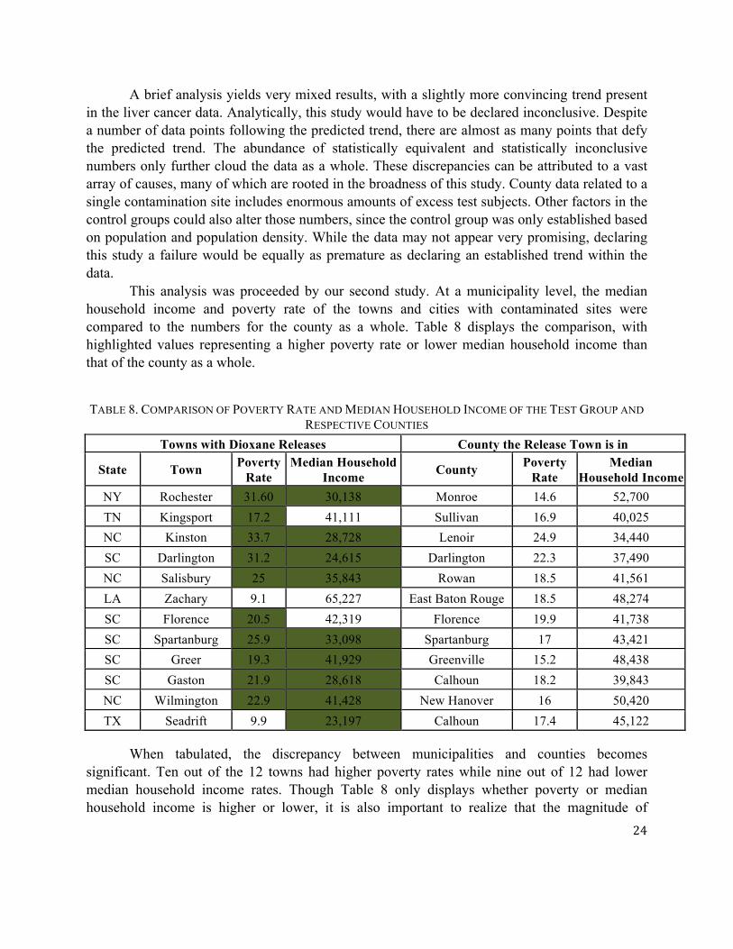
This analysis was proceeded by our second study. At a municipality level, the median household income and poverty rate of the towns and cities with contaminated sites were compared to the numbers for the county as a whole. Table 8 displays the comparison, with highlighted values representing a higher poverty rate or lower median household income than that of the county as a whole.

 

TABLE 8. COMPARISON OF POVERTY RATE AND MEDIAN HOUSEHOLD INCOME OF THE TEST GROUP AND RESPECTIVE COUNTIES

Towns with Dioxane Releases County the Release Town is in

State Town Poverty Rate

Median Household Income County Poverty

Rate Median

Household Income NY Rochester 31.60 30,138 Monroe 14.6 52,700 TN Kingsport 17.2 41,111 Sullivan 16.9 40,025 NC Kinston 33.7 28,728 Lenoir 24.9 34,440 SC Darlington 31.2 24,615 Darlington 22.3 37,490 NC Salisbury 25 35,843 Rowan 18.5 41,561 LA Zachary 9.1 65,227 East Baton Rouge 18.5 48,274 SC Florence 20.5 42,319 Florence 19.9 41,738 SC Spartanburg 25.9 33,098 Spartanburg 17 43,421 SC Greer 19.3 41,929 Greenville 15.2 48,438 SC Gaston 21.9 28,618 Calhoun 18.2 39,843 NC Wilmington 22.9 41,428 New Hanover 16 50,420 TX Seadrift 9.9 23,197 Calhoun 17.4 45,122

When tabulated, the discrepancy between municipalities and counties becomes significant. Ten out of the 12 towns had higher poverty rates while nine out of 12 had lower median household income rates. Though Table 8 only displays whether poverty or median household income is higher or lower, it is also important to realize that the magnitude of

25      

 

difference between the town and county is variably drastic. Poverty rates range from almost statistically equivalent to double that of the county as a whole (Rochester: Monroe). Likewise, median household income in contaminated municipalities is sometimes nearly half that of the county (Seadrift: Calhoun).

As shown in figure 9 and 10, created from data provided by the Rural Assistance Center, contamination is almost exclusively located in the South. Likewise, it accurately trends along with both lower median household income and higher poverty rates. When shown in contrast to the rest of the counties of the United States, the reciprocal of this becomes strikingly more apparent: the wealthier and less impoverished counties have virtually no dioxane contamination sites.

 FIGURE 9. MEDIAN HOUSEHOLD INCOME BY COUNTY ( RURAL ASSISTANCE CENTER, 2011)

 

FIGURE 10. POVERTY RATE BY COUNTY (RURAL ASSISTANCE CENTER, 2011)

26      

 

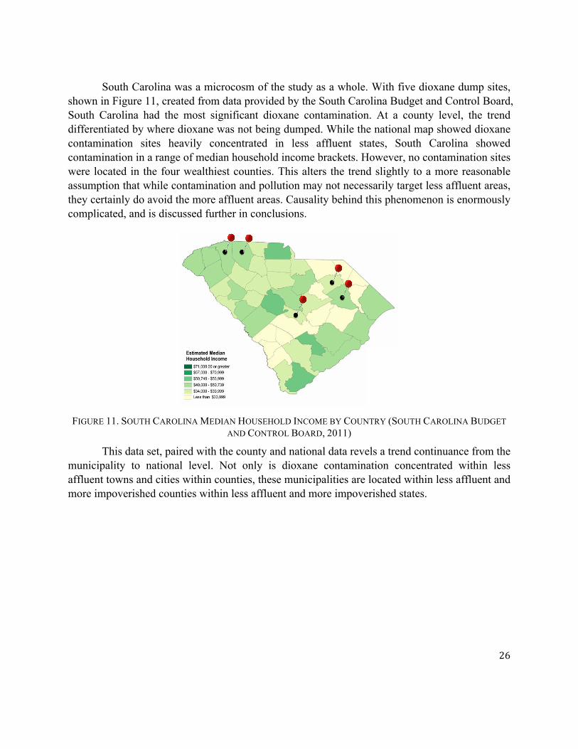
   South Carolina was a microcosm of the study as a whole. With five dioxane dump sites,

shown in Figure 11, created from data provided by the South Carolina Budget and Control Board, South Carolina had the most significant dioxane contamination. At a county level, the trend differentiated by where dioxane was not being dumped. While the national map showed dioxane contamination sites heavily concentrated in less affluent states, South Carolina showed contamination in a range of median household income brackets. However, no contamination sites were located in the four wealthiest counties. This alters the trend slightly to a more reasonable assumption that while contamination and pollution may not necessarily target less affluent areas, they certainly do avoid the more affluent areas. Causality behind this phenomenon is enormously complicated, and is discussed further in conclusions.  

 

FIGURE 11. SOUTH CAROLINA MEDIAN HOUSEHOLD INCOME BY COUNTRY (SOUTH CAROLINA BUDGET AND CONTROL BOARD, 2011)

This data set, paired with the county and national data revels a trend continuance from the municipality to national level. Not only is dioxane contamination concentrated within less affluent towns and cities within counties, these municipalities are located within less affluent and more impoverished counties within less affluent and more impoverished states.

   

27      

 

Plug-Flow Reactor Design This section outlines the design of a plug-flow reactor for the EPA superfund site in Westville, IN. The current superfund site has recorded dioxane contamination levels between 6 mg/L and 10 mg/L. The area of the contamination site is approximately 15 acres and sits north of the Indiana State Route 2 and one-quarter mile from U.S. Highway 421. Surrounding the contamination site are a residential neighborhood, agricultural land, an abandoned railroad easement, and an auto salvage yard. From 1934 to 1987 the site was used to collect, store, and re-refine waste oil by the Westville Oil Division of Cam-Or. Westville Oil collected wastes from sources such as service stations, industrial facilities, railroad yards, and pipelines to re-refine the oil and use it in automotive- and industrial-grade lubrication oil blends (U.S. EPA, 2014b). In 1959, the company constructed a lagoon for waste storage, disposal, and separation of oil and water fractions. These lagoons were constructed using sandy soils without liners to prevent the waste seeping into the underlying soils and groundwater. Lagoons were utilized until 1978 when the fish in Crooked Creek, upstream of the contamination site, were killed due to chemical contamination from the site. In 1987, the United States EPA initiated a removal action through the Emergency Removal Program to mitigate the imminent threat posed by the contamination site (U.S. EPA, 2014b). The contamination site has approximately 10.5 million gallons of water contaminated with 6-10 mg/L of dioxane. To treat the dioxane levels in the water within three years, 10,000 gallons per day (gpd) will need to be processed and piped off site to reenter the aquifers. The plug-flow reactor was designed with the following assumptions:

• The plug-flow reactor will operate at a steady state • The dioxane degrades based upon a first-order kinetic reaction • The treatment process will be completed within three years (the system was designed

based upon this assumption) The water from the aquifers will need to be pumped above ground to be treated, mixed

with H2O2, and flow through a plug-flow reactor with UV lamp treatment. The flow rate of the water was calculated based upon the amount of water on site and the desired time frame for treatment. First, the design flowrate was calculated as seen in Equation 4:

𝑓𝑙𝑜𝑤𝑟𝑎𝑡𝑒 = !",!"",!!!  !"##$%&

!  !"#$%!  !"#$!"#  !"#$

!  !"#!"  !!"#$

!  !!"#!"  !"#

(Equation 4)

= 𝟔.𝟗𝟓𝒈𝒂𝒍𝒎𝒊𝒏 ≈ 𝟕

𝒈𝒂𝒍𝒎𝒊𝒏

28      

 

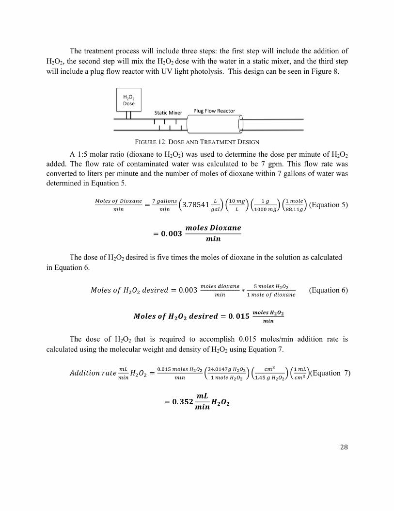
The treatment process will include three steps: the first step will include the addition of H2O2, the second step will mix the H2O2 dose with the water in a static mixer, and the third step will include a plug flow reactor with UV light photolysis. This design can be seen in Figure 8.

 FIGURE 12. DOSE AND TREATMENT DESIGN

  A 1:5 molar ratio (dioxane to H2O2) was used to determine the dose per minute of H2O2

added. The flow rate of contaminated water was calculated to be 7 gpm. This flow rate was converted to liters per minute and the number of moles of dioxane within 7 gallons of water was determined in Equation 5.

!"#$%  !"  !"#$%&'

!"#= !  !"##$%&

!"#3.78541 !

!"#!"  !"!

!  !!"""  !"

!  !"#$!!.!!!

(Equation 5)

= 𝟎.𝟎𝟎𝟑  𝒎𝒐𝒍𝒆𝒔  𝑫𝒊𝒐𝒙𝒂𝒏𝒆

𝒎𝒊𝒏

The dose of H2O2 desired is five times the moles of dioxane in the solution as calculated

in Equation 6.

𝑀𝑜𝑙𝑒𝑠  𝑜𝑓  𝐻!𝑂!  𝑑𝑒𝑠𝑖𝑟𝑒𝑑 = 0.003  !"#$%  !!"#$%&!"#

∗ !  !"#$%  !!!!!  !"#$  !"  !"#$%&'

(Equation 6)

𝑴𝒐𝒍𝒆𝒔  𝒐𝒇  𝑯𝟐𝑶𝟐  𝒅𝒆𝒔𝒊𝒓𝒆𝒅 = 𝟎.𝟎𝟏𝟓  𝒎𝒐𝒍𝒆𝒔  𝑯𝟐𝑶𝟐

𝒎𝒊𝒏

The dose of H2O2 that is required to accomplish 0.015 moles/min addition rate is

calculated using the molecular weight and density of H2O2 using Equation 7.

𝐴𝑑𝑑𝑖𝑡𝑖𝑜𝑛  𝑟𝑎𝑡𝑒 !"!"#

𝐻!𝑂! =!.!"#  !"#$%  !!!!

!"#!".!"#$!  !!!!!  !"#$  !!!!

!"!

!.!"  !  !!!!

!  !"!"! (Equation 7)

= 𝟎.𝟑𝟓𝟐𝒎𝑳𝒎𝒊𝒏𝑯𝟐𝑶𝟐

29      

 

This calculation assumes a 100% H2O2 solution; therefore, if the stock solution of H2O2 is less than 100%, the dose will need to be changed accordingly. For example, for a 30% stock solution of H2O2, the required volume per minute can be calculated using Equation 8.

𝐷𝑜𝑠𝑒  𝐷𝑒𝑠𝑖𝑟𝑒𝑑  𝑓𝑜𝑟  30%  𝑆𝑡𝑜𝑐𝑘  𝑆𝑜𝑙𝑢𝑡𝑖𝑜𝑛 = 0.352 !"!"#

𝐻!𝑂!!""!"% (Equation 8)

= 𝟏.𝟏𝟕  𝑯𝟐𝑶𝟐𝒎𝑳𝒎𝒊𝒏

The H2O2 will be added to the water prior to the static mixer to ensure that the H2O2 will

be fully mixed within the solution before it enters the plug-flow reactor. A static mixer is added to the pipeline with the objective of manipulating the water stream to divide, recombine, accelerate/decelerate, spread, and swirl the water as it passes through the mixer. A static mixer is chosen for its low cost and maintenance and utilized when inexpensive and fast operation is required. The static mixer includes several baffles that move and circulate the water and mix with the H2O2.

After the water passes through the static mixer, it will be piped into the plug-flow reactor. To determine the plug-flow reactor size, a material balance of the system was determined shown in Equation 9.

𝑄 !"!"= −𝑘𝐶 (Equation 9)

This equation was then integrated:

𝑑𝑐𝐶

!!

!!= −

𝑘𝑄 𝑑𝑣

!

!

ln𝐶!𝐶!

= −𝑘𝑉𝑄

CO and Cf are the initial and final concentration of dioxane respectively, v is the volume

of the plug flow reactor and k is the kinetic constant determined experimentally in the results section to be 0.15 min-1. The initial concentration of dioxane provided by the EPA is 6-10 mg/L however the treatment process assumes a concentration of 10 mg/L. The treatment process aims for 99 percent removal of dioxane leaving a final concentration of 0.1 mg/L dioxane. Therefore, the volume of the reactor was calculated in Equation 10.

30      

 

ln !.!  !"/!!"  !"/!

= − (!.!"/!"#)!!  !"#  /!"#

(Equation 10)

𝑽 = 𝟐𝟏𝟓  𝒈𝒂𝒍  

The contact time of the reactor was also determined from a material balance of the

system, as shown in Equation 11.

!"!"= −𝑘𝐶 (Equation 11)

This equation was then integrated as seen in Equation 12:

!"!

!!!!

= −𝑘 𝑑𝑡!! (Equation 12)

ln𝐶!𝐶!

= −𝑘𝑡

CO and Cf are the initial and final concentration of dioxane respectively, t is the detention

time in the reactor, and k is the kinetic constant determined experimentally in the results section to be 0.15 min-1. Therefore, the detention time of the reactor was calculated in Equation 13:

ln !.!  !"/!!"  !"/!

= −(0.15/min  )𝑡 (Equation 13)

𝒕 = 𝟑𝟏  𝒎𝒊𝒏

The plug-flow reactor will have a volume of 215 gallons and a detention time of 31

minutes. The power required for treatment can be calculated using the ratio of energy needed to treat the 12 mL sample in the laboratory and the volume of water in the reactor. First, the volume of the reactor was converted to liters in Equation 14.

215  𝑔𝑎𝑙 3.78541 !

!"#= 814  𝐿 (Equation 14)

A ratio of mL/watts was then used to determine the energy required for the treatment

system using Equation 15.

31      

 

!.!  !"##$!.!"#  !

= !"#$%  (!"#$$%)!"#  !

(Equation 15)

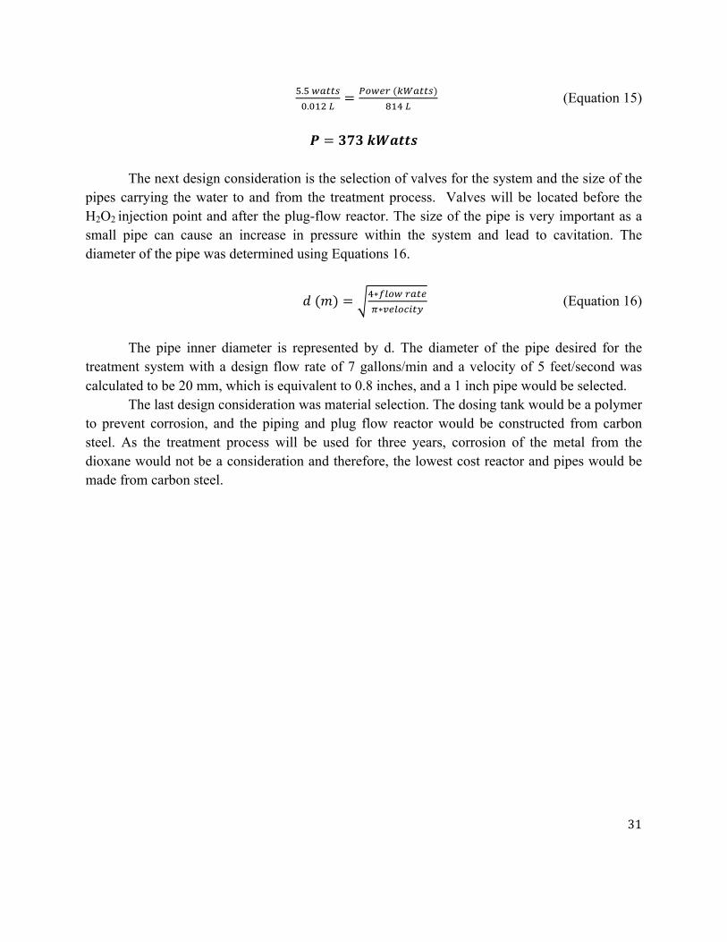
𝑷 = 𝟑𝟕𝟑  𝒌𝑾𝒂𝒕𝒕𝒔 The next design consideration is the selection of valves for the system and the size of the

pipes carrying the water to and from the treatment process. Valves will be located before the H2O2 injection point and after the plug-flow reactor. The size of the pipe is very important as a small pipe can cause an increase in pressure within the system and lead to cavitation. The diameter of the pipe was determined using Equations 16.

𝑑  (𝑚) = !∗!"#$  !"#$!∗!"#$%&'(

(Equation 16)

The pipe inner diameter is represented by d. The diameter of the pipe desired for the

treatment system with a design flow rate of 7 gallons/min and a velocity of 5 feet/second was calculated to be 20 mm, which is equivalent to 0.8 inches, and a 1 inch pipe would be selected.

The last design consideration was material selection. The dosing tank would be a polymer to prevent corrosion, and the piping and plug flow reactor would be constructed from carbon steel. As the treatment process will be used for three years, corrosion of the metal from the dioxane would not be a consideration and therefore, the lowest cost reactor and pipes would be made from carbon steel.

 

32      

 

Conclusions and Recommendations In whatever form the remediation process may take, the use of H2O2 and UV light does

show conclusive evidence for the removal of dioxane. In order to optimize efficiency, this design should utilize a 1:5 molar ratio of dioxane to H2O2, a contact time of 15 minutes, while operating at a pH of 7. These levels should not only be compared to other remediation techniques, but also examined to potentially retrofit any existing remediation systems. The design portion of this project shows that our specific design could be implemented at a remediation site strictly for the remediation of dioxane but a current system for on-site treatment of volatile organic compounds could be modified to include the UV/H2O2 system.

To enhance this study, tests should be conducted with a dioxane concentration greater than 5 mg/L to emulate the observed concentrations found in contamination sites currently being remediated (Office of Solid Waste and Emergency Response, 2006). This study could also be enhanced by the addition of experiments varying pH over all ratios to determine if adjustment in pH can increase the efficiency of a lower dose of H2O2.

As certain states and counties begin to clean up dioxane contamination, others continue to release dioxane. A first step toward any sort of remediation would be preventing the need for further remediation by reducing or suspending current dioxane dumping locations. Having government organizations provide more substantial and convincing evidence linking dioxane to chronic and acute illnesses could advance this effort.

This directly leads into the connection between the engineering and social scientific portions of this project. More direct and convincing results connecting medical data to the presence of dioxane could verify the epidemiological danger of dioxane contamination, and, in turn, provide the evidence necessary to convince municipalities and states to prevent further dioxane dumping. This could be established using a modified version of our initial analytic study.

A modified version of the first study could provide the evidence necessary to support medical claims of dioxane danger with comprehensive, univocal, empirical data. While this initial study was statistically inconclusive, there are a number of strategies that could be employed to modify this strategy, assuming that there is the data to match the presumption. Focusing the study to a smaller segment of the population, such as those living within a specific distance from the contamination site, could provide more accurate and distinct data. Using this sort of study as a pilot plan could streamline the entire process into a model that could be implemented at each individual contamination site. A more distinct trend with a more lucid methodology, could considerably improve this portion of the study.

The success of the second study illustrates the potential of a wider study to more accurately examine the connection between social factors and the presence of pollution. Expansion of this second study could be equally as impactful as the first, just on a much wider scale. This study very convincingly established a trend between the presence of dioxane and poverty. It would be illogical to assume that the presence of dioxane habitually leads to the creation or sustenance of poverty. Inversely, the notion that polluters actively target less wealthy communities is more evenhanded. This trend could be empirically established by increasing the second study to include multiple pollutants. It would be fascinating to examine the correlation between the presence of pollution and the rate of poverty of a community, especially over a

33      

 

historic phase. If the second study is any indication of what this theoretical study would confirm, it could reasonably anticipated that a national or, (resource permitting) global trend between the presence of pollution and social determents would be revealed. The reciprocal of this would likely again be observed with a lack or absence of heavy and dangerous pollution taking place within wealthy countries or regions.

 

34      

 

Works Cited Agency for Toxic Substances and Disease Registry. Division of Toxicology and Human Health

Sciences. (2012). Public Health Statement 1,4-Dioxane. Atlant, GA. (CAS # 123-91-1)

Avisar, D., Lester, Y., & Mamane, H. (2010). pH induced polychromatic UV treatment for the removal of a mixture of SMX, OTC and CIP from water. Journal of Hazardous Materials, 1068-1074.

Buffler, P. A., Wood, S. M., Suarez, L., & Kilian, D. J. (1978). Mortality follow-up of workers exposed to 1,4-dioxane. Journal of Occupational and Environmental Medicine, 20(4), 255-259.

Department of Health and Human Services (2011). Report on Carcinogens (No. 1437987362). Darby, PA: DIANE Publishing.

Calabrese, E.J and Kenyon, K.M (1991). Air Toxics and Risk Assessment. Lewis Publishers, Chelsea, MI.

Herruzo C, R.; Arrazola, A.L.; Alcaide, V.; Arjona, M.F.; CAlero, J.R (1994). “Analytic Epidemiology of Clinical Urinary Tract Infection in Spinal Cord Injury.” European journal of epidemiology 10.1: 23-7.

International Agency for Research on Cancer (1987 ). 1,4 Dioxane. Lyon, France.

IJpelaar, G., Harmsen, D., & Heringa, M. (2007). UV disinfection and UV/H2O2 oxidation: by-product formation and control. Natick, MA: Techneau.

Matlis, J (2006). Predictive Analytics. 40 Vol. Framingham: Computerworld, Inc,

Office of Solid Waste and Emergency Response (2006). Treatment Technologies for 1,4-Dioxane: Fundamentals and Field Applications. EPA. Cincinnati, OH.

Pereira, V. J., Linden, K. G., & Weinberg, H. S. (2007). Evaluation of UV irradiation for photolytic and oxidative degradation of pharmaceutical compounds in water. Water Research, 4413-4423.

Runkler, Thomas A., and SpringerLink ebooks - Computer Science. Data Analytics (2012): Models and Algorithms for Intelligent Data Analysis. New York: Vieweg Teubner Verlag,

Rural Assistance Center (GIS Service). (2011a) Estimated Median Household Income [Map], Retrieved April 5, 2014, from: http://www.raconline.org/racmaps/

35      

 

Rural Assistance Center (GIS Service). (2011b) Estimated Percent of Population in Pverty: All Ages by County [Map], Retrieved April 5, 2014, from: http://www.raconline.org/racmaps/

South Carolina Budget and Control Board (Community Profiles). (2007) Median Household Income [Map], Retrieved April 5, 2014, from:  http://www.sccommunityprofiles.org/saipe/mhi07.php

Stephenson, D. (2000) Brief History of Statistics; University of Reading: Reading, U.K.

Stuart, B., Prichard, E. (2003). Practical Laboratory Skills Training Guides: Gas Chromatography. Gas Chromatography

Thiess, A. M., Tress, E., & Fleig, I. (1976). Arbeitsmedizinische Untersuchungsergebnisse von Dioxan-exponierten Mitarbeitern [Industrial-medical investigation results in the case of workers exposed to dioxane]. Arbeitsmedizin, Sozialmedizin, Umweltmedizin, 11, 35-46.

U.S. EPA (2000). 1,4-Dioxane (1,4-Diethyleneoxide). From http://www.epa.gov/fedfac/pdf/technical_fact_sheet_14-dioxane_2013.pdf

U.S. EPA (2013a). ATSDR - ToxFAQs™: 1,4-Dioxane. Retrieved From http://www.atsdr.cdc.gov/toxfaqs/tf.asp?id=954&tid=199

U.S. EPA (April 2014).Contaminated Site Clean-Up Information. 1,4-dioxane: Detection and Site Characterization. Retrieved From http://www.cluin.org/contaminantfocus/default. focus/sec/1,4-dioxane/cat/Detection_and_Site_Characterization/

U.S. EPA (April 2014b) Superfund Site Progress Profile CAM-OR INC. (EPA ID:IND005480462) Retrieved From: http://cumulis.epa.gov/supercpad/cursites/ csitinfo.cfm?id=0501297

U.S. EPA (2013b). Technical Fact Sheet – 1,4-Dioxane. Retrieved From http://www.epa.gov/fedfac/pdf/technical_fact_sheet_14-dioxane_2013.pdf

U.S. EPA (2013c). Toxicological Review for 1-4-Dioxane (with Inhalation Update) September 2013 - 0326tr.pdf. from http://www.epa.gov/iris/toxreviews/0326tr.pdf

U.S. EPA; Office of Environmental Information, Office of Information Analysis and Access, Toxice Release Inventory Program Division & Information and Outreach Branch (2013d). Toxic Release Inventory Basic Data File Format Documentation v12.

Work Environment Toxicology, Institute of Environmental Medicine, Karolinska Institutet, Stockholm, Sweden. (2006). Acute effects of exposure to vapors of dioxane in humans. Human & Experimental Toxicology, 25(12), 723-729.

36      

 

World Health Organization. (2005). 1,4 Dioxane in Drinking-Water. Copenhagen.

Yoshinaga, J.; Tamura, M. (1995). Explosion During Transfer of Dioxane by Compressed Air. Retrieved from http://www.sozogaku.com/fkd/en/cfen/CC1000015.html

 

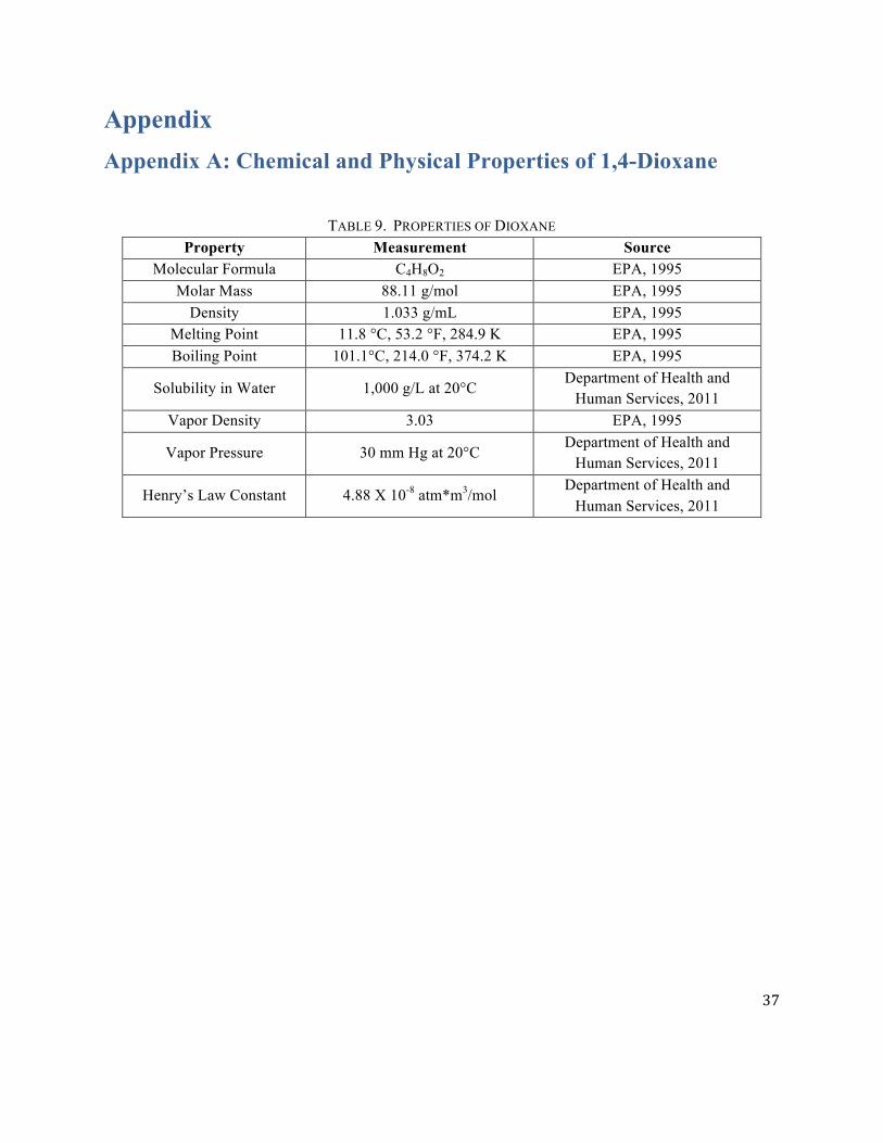
37      

 

Appendix Appendix A: Chemical and Physical Properties of 1,4-Dioxane

 

TABLE 9. PROPERTIES OF DIOXANE Property Measurement Source

Molecular Formula C4H8O2 EPA, 1995 Molar Mass 88.11 g/mol EPA, 1995

Density 1.033 g/mL EPA, 1995 Melting Point 11.8 °C, 53.2 °F, 284.9 K EPA, 1995 Boiling Point 101.1°C, 214.0 °F, 374.2 K EPA, 1995

Solubility in Water 1,000 g/L at 20°C Department of Health and

Human Services, 2011 Vapor Density 3.03 EPA, 1995

Vapor Pressure 30 mm Hg at 20°C Department of Health and

Human Services, 2011

Henry’s Law Constant 4.88 X 10-8 atm*m3/mol Department of Health and

Human Services, 2011

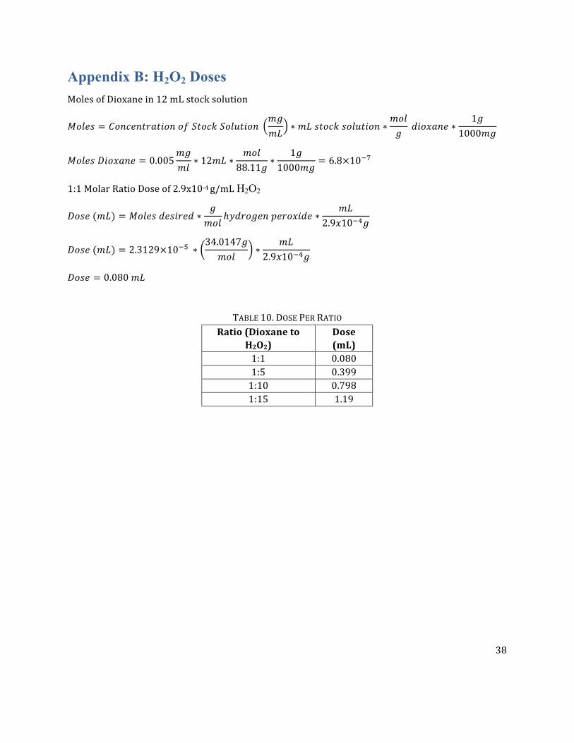
38      

 

Appendix B: H2O2 Doses Moles  of  Dioxane  in  12  mL  stock  solution  

𝑀𝑜𝑙𝑒𝑠 = 𝐶𝑜𝑛𝑐𝑒𝑛𝑡𝑟𝑎𝑡𝑖𝑜𝑛  𝑜𝑓  𝑆𝑡𝑜𝑐𝑘  𝑆𝑜𝑙𝑢𝑡𝑖𝑜𝑛  𝑚𝑔𝑚𝐿

∗𝑚𝐿  𝑠𝑡𝑜𝑐𝑘  𝑠𝑜𝑙𝑢𝑡𝑖𝑜𝑛 ∗𝑚𝑜𝑙𝑔

 𝑑𝑖𝑜𝑥𝑎𝑛𝑒 ∗1𝑔

1000𝑚𝑔  

𝑀𝑜𝑙𝑒𝑠  𝐷𝑖𝑜𝑥𝑎𝑛𝑒 = 0.005𝑚𝑔𝑚𝑙

∗ 12𝑚𝐿 ∗𝑚𝑜𝑙

88.11𝑔∗

1𝑔1000𝑚𝑔

= 6.8×10!!  

1:1  Molar  Ratio  Dose  of  2.9x10-­‐4  g/mL  H2O2  

𝐷𝑜𝑠𝑒  (𝑚𝐿) = 𝑀𝑜𝑙𝑒𝑠  𝑑𝑒𝑠𝑖𝑟𝑒𝑑 ∗𝑔𝑚𝑜𝑙

ℎ𝑦𝑑𝑟𝑜𝑔𝑒𝑛  𝑝𝑒𝑟𝑜𝑥𝑖𝑑𝑒 ∗𝑚𝐿

2.9𝑥10!!𝑔  

𝐷𝑜𝑠𝑒  (𝑚𝐿) = 2.3129×10!!   ∗34.0147𝑔𝑚𝑜𝑙

∗𝑚𝐿

2.9𝑥10!!𝑔  

𝐷𝑜𝑠𝑒 = 0.080  𝑚𝐿  

 

TABLE  10.  DOSE  PER  RATIO  Ratio  (Dioxane  to  

H2O2)  Dose  (mL)  

1:1   0.080  1:5   0.399  1:10   0.798  1:15   1.19  

 

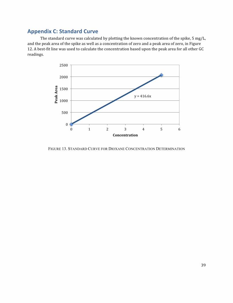
39      

 

Appendix  C:  Standard  Curve     The  standard  curve  was  calculated  by  plotting  the  known  concentration  of  the  spike,  5  mg/L,  and  the  peak  area  of  the  spike  as  well  as  a  concentration  of  zero  and  a  peak  area  of  zero,  in  Figure  12.  A  best-­‐fit  line  was  used  to  calculate  the  concentration  based  upon  the  peak  area  for  all  other  GC  readings.  

 

FIGURE 13. STANDARD CURVE FOR DIOXANE CONCENTRATION DETERMINATION

   

y  =  416.6x  

0  

500  

1000  

1500  

2000  

2500  

0   1   2   3   4   5   6  

Peak  Area  

Concentration  

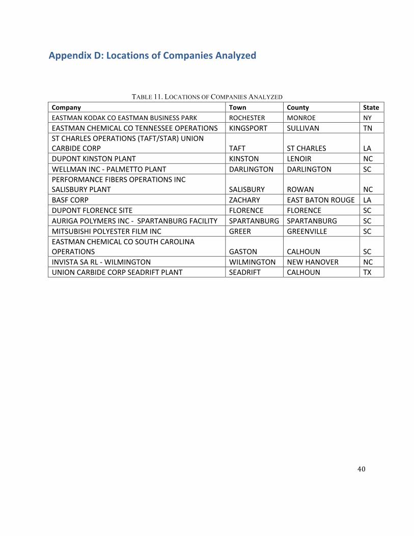
40      

 

Appendix  D:  Locations  of  Companies  Analyzed    

 

TABLE 11. LOCATIONS OF COMPANIES ANALYZED Company   Town   County   State  EASTMAN  KODAK  CO  EASTMAN  BUSINESS  PARK   ROCHESTER   MONROE   NY  EASTMAN  CHEMICAL  CO  TENNESSEE  OPERATIONS   KINGSPORT   SULLIVAN   TN  ST  CHARLES  OPERATIONS  (TAFT/STAR)  UNION  CARBIDE  CORP   TAFT   ST  CHARLES   LA  DUPONT  KINSTON  PLANT   KINSTON   LENOIR   NC  WELLMAN  INC  -­‐  PALMETTO  PLANT   DARLINGTON   DARLINGTON   SC  PERFORMANCE  FIBERS  OPERATIONS  INC  SALISBURY  PLANT   SALISBURY   ROWAN   NC  BASF  CORP   ZACHARY   EAST  BATON  ROUGE   LA  DUPONT  FLORENCE  SITE   FLORENCE   FLORENCE   SC  AURIGA  POLYMERS  INC  -­‐    SPARTANBURG  FACILITY   SPARTANBURG   SPARTANBURG   SC  MITSUBISHI  POLYESTER  FILM  INC   GREER   GREENVILLE   SC  EASTMAN  CHEMICAL  CO  SOUTH  CAROLINA  OPERATIONS   GASTON   CALHOUN   SC  INVISTA  SA  RL  -­‐  WILMINGTON   WILMINGTON   NEW  HANOVER   NC  UNION  CARBIDE  CORP  SEADRIFT  PLANT   SEADRIFT   CALHOUN   TX  

     

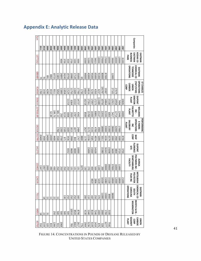
41      

 

Appendix  E:  Analytic  Release  Data      

Companies

EASTMAN0

KODAK0CO0EASTM

AN0BUSINESS0PARK

EASTMAN0

CHEMICAL0CO0

TENNESSEE0OPERATIONS

ST0CHARLES0OPERATIONS0(TAFT/STAR)0

UNION0CARBIDE0CORP

DUPONT0KINSTON0PLANT

WELLM

AN0INC0@0

PALMETTO0

PLANT

PERFORMANC

E0FIBERS0OPERATIONS0

INC0SALISBURY0PLANT

BASF0CORP

DUPONT0FLORENCE0

SITE

AURIGA0POLYM

ERS0INC0@00SPARTANBURG0

FACILITY

MITSUBISHI0

POLYESTER0FILM

0INC

EASTMAN0

CHEMICAL0CO0

SOUTH0CAROLINA0

OPERATIONS

INVISTA0SA0RL0@0WILM

INGTON

UNION0CARBIDE0CORP0

SEADRIFT0PLANT

198781000

1060624000

87003700

210001988

1200007494

1244617000

33003720

1100018900

1989140000

2707914958

1271432000

29003800

1600012000

199099000

1200027102

129215417

280002000

360037000

1890038000

1991160000

151006003

310006579

1569839000

151008900

31007546

1992170000

8700019387

1486431593

330006336

1634320000

1508013000

17006277

1993270000

80000193787

1075622032

180005011

15380200

1010011000

2000328

1994130000

910004237

11348023147

49005099

11005439

3702400

8761995

5602365000

435017273

308914700

497414100

5002896

2507240

14591996

4400995000

523017097

164004143

358515000

4004820

1608100

31491997

5100043000

1461617261

157003172

1233615000

270110

53405236

199832000

4400014604

162188500

26271170

130200

41301944

199965

17308800

1075776

20005000

3500017700

147374342

24841747

10000131

1608790

26172001

530017149

1160015332

37871877

8438000

131250

89204663

20022700

1998011750

63642920

18152908

8600131

25010010

7832003

350019706

1152911154

30081600

34368332

250250

5002004

370024240

118583219

2100671

250130

5002005

400024893

11800250

22002700

250500

20682006

118055050

385.121700

2500250

15500

9152007

107259311

199.734400

43022

2501266

20084865

441062.84

14000490

11833

2009891

429024000

200015

31320

201091

14303400

106718

222144

201175

170020400

134718

550Sum

1377232686485

414550315615

227016.69192318

151795141273

133402124235

7311164051

43750

FIGURE 14. CONCENTRATIONS IN POUNDS OF DIOXANE RELEASED BY UNITED STATES COMPANIES

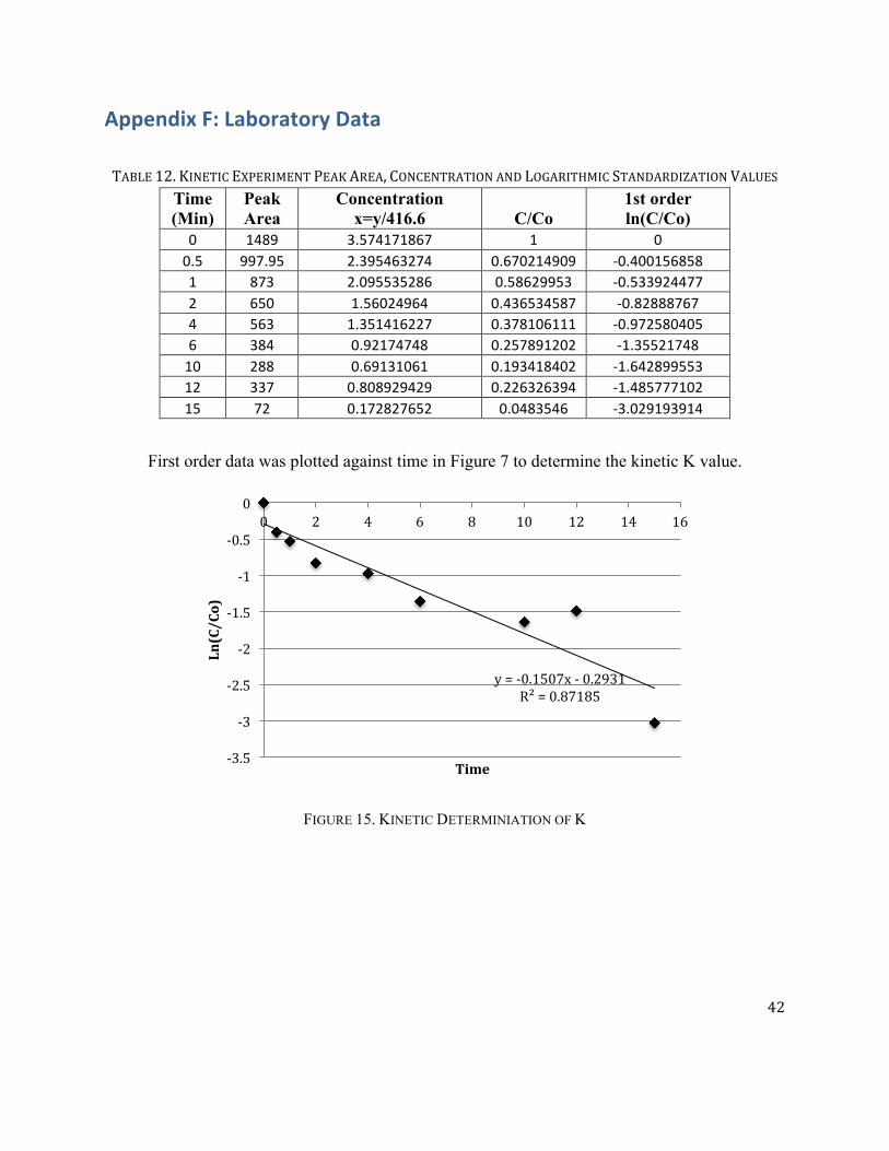
42      

 

Appendix  F:  Laboratory  Data      

TABLE  12.  KINETIC  EXPERIMENT  PEAK  AREA,  CONCENTRATION  AND  LOGARITHMIC  STANDARDIZATION  VALUES  Time (Min)

Peak Area

Concentration x=y/416.6 C/Co

1st order ln(C/Co)

0   1489   3.574171867   1   0  0.5   997.95   2.395463274   0.670214909   -­‐0.400156858  1   873   2.095535286   0.58629953   -­‐0.533924477  2   650   1.56024964   0.436534587   -­‐0.82888767  4   563   1.351416227   0.378106111   -­‐0.972580405  6   384   0.92174748   0.257891202   -­‐1.35521748  10   288   0.69131061   0.193418402   -­‐1.642899553  12   337   0.808929429   0.226326394   -­‐1.485777102  15   72   0.172827652   0.0483546   -­‐3.029193914  

 

First order data was plotted against time in Figure 7 to determine the kinetic K value.

 

FIGURE 15. KINETIC DETERMINIATION OF K

   

   

y  =  -­‐0.1507x  -­‐  0.2931  R²  =  0.87185  

-­‐3.5  

-­‐3  

-­‐2.5  

-­‐2  

-­‐1.5  

-­‐1  

-­‐0.5  

0  0   2   4   6   8   10   12   14   16  

Ln(C/Co)  

Time