Embed Size (px)
Citation preview

Centre for the Analysis of Risk and
Optimisation Modelling Applications
CTR/26/03 May 2004
Treasury Management Model with Foreign Exchange Exposure
Konstantin Volosov, Gautam Mitra, Fabio Spagnolo,
Cormac Lucas.
CARISMA
A multi-disciplinary research centre focussed on
understanding, modelling, quantification, management and
control of RISK
Centre for the Analysis of Risk and
Optimisation Modelling Applications
TECHNICAL REPORT
Department of Mathematical Sciences and Department of Economics and Finance
Brunel University, Uxbridge, Middlesex, UB8 3PH timisatio
Treasury Management Model with Currency Exposure
2
Abstract
In this paper we formulate a model for foreign exchange exposure management and (international)
cash management taking into consideration random fluctuations of exchange rates. A vector error
correction model (VECM) is used to predict the random behaviour of the forward as well as spot
rates connecting dollar and sterling. A two-stage stochastic programming (TWOSP) decision model
is formulated using these random parameter values. This model computes currency hedging
strategies, which provide rolling decisions of how much forward contracts should be bought and
how much should be liquidated. The model decisions are investigated through ex post simulation
and backtesting in which value at risk (VaR) for alternative decisions are computed. The
investigation (a) shows that there is a considerable improvement to “spot only” strategy, (b)
provides insight into how these decisions are made and (c) also validates the performance of this
model.
Treasury Management Model with Currency Exposure
3
Table of Contents
Abstract ..............................................................................................................................2
1 Introduction and Background ................................................................................4
2 Modelling Stochastic Processes ...........................................................................9
2.1 The Exchange Rates: A Model of Cointegration between Spots and Forwards. 9
2.2 Comparing Alternative Models and Model Validation......................................... 11
2.3 Scenario Generation .............................................................................................. 14
2.4 The Scenario Tree .................................................................................................. 14
3 The Problem Setting .............................................................................................16
3.1 Two Stage SP Model with Recourse..................................................................... 16
3.2 The SP Decision Model.......................................................................................... 17
4 Backtesting and Rolling forward the SP Decision Model ..................................26
4.1 Dynamic Data Model .............................................................................................. 27
4.2 The Rolling Decision Model .................................................................................. 28
4.3 Simulation 1: Risk and Return Analysis .............................................................. 29
4.4 Simulation 2: Stochastic Measures ...................................................................... 35
5 Conclusions...........................................................................................................37
6 References.............................................................................................................38
Appendix A: Choice of Risk Measures ..........................................................................41
Appendix B: Metallgesellschaft A.G. Example..............................................................44
Appendix C: SP Model Definition and Stochastic Measures .......................................45
Treasury Management Model with Currency Exposure
4
1 Introduction and Background
Foreign Exchange (FX) markets have gone through a turbulent period since 1973 (after the collapse
of Bretton Woods). More recently since 1999 with the emergence of the euro as well as increased
globalisation of trade a spectacular amount of currency movement has been recorded. In her recent
book Taylor (2003) reports that more than 1.2 trillion USD change hands daily on the foreign
exchanges. It is therefore only natural that FX management has become an important topic
especially so over the last decade.
The FX participants can be grouped into four categories. (i) The first participants are domestic and
international banks, which act on their own behalf and for their customers. (ii) The second group
comprise the Central banks, which may intervene in the market in order to support or suppress the
value of the domestic currency for reserve management purposes. (iii) The third group is made up
of multinational firms (MNFs) who are the customers of banks and buy physical currency in the
spot or forward FX market for the purposes of facilitating trade. These MNFs buy and sell foreign
currency. (iv) The fourth group includes the individual or corporate speculators or traders. In
general FX decisions can be seen from two perspectives, such as: (a) hedgers and (b) speculators or
traders. In this paper we use the term trader and speculator interchangeably from now on.
The currency management undertaken by multinational firms (MNF) constitutes only a small
fraction (5% – 10%) of total FX transactions. Yet for the purpose of treasury management hedging
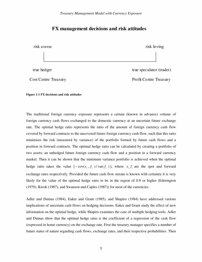
and limited trading are of vital importance to the corporations and FX decisions can be categorised
as shown in Figure 1-1, Taylor (2003). Whereas introducing some element of FX trader (speculator)
approach may lead to a better FX decision making there are natural pitfalls for an MNF should it
move too far to the right of the scale shown in Figure 1-1. The well-known case of
Metallgesellschaft A.G. (see Appendix B) is one of a few notorious examples of the plight of MNFs
who ventured into FX trading activities largely from the position of a speculator. In this paper we
are concerned with risk exposure of a multinational firm (MNF) and treasury risk management
requirement in respect of FX exposure.
Treasury Management Model with Currency Exposure
5
FX management decisions and risk attitudes
risk averse risk loving
true hedger
Cost Centre Treasury
true speculator (trader)
Profit Centre Treasury
Figure 1-1 FX decisions and risk attitudes
The traditional foreign currency exposure represents a certain (known in advance) volume of
foreign currency cash flows exchanged to the domestic currency at an uncertain future exchange
rate. The optimal hedge ratio represents the ratio of the amount of foreign currency cash flow
covered by forward contracts to the uncovered future foreign currency cash flow, such that this ratio
minimises the risk (measured by variance) of the portfolio formed by future cash flows and a
position in forward contracts. The optimal hedge ratio can be calculated by creating a portfolio of
two assets: an unhedged future foreign currency cash flow and a position in a forward currency
market. Then it can be shown that the minimum variance portfolio is achieved when the optimal
hedge ratio takes the value [ )var(/),cov( ttt ffs− ], where tt fs , are the spot and forward
exchange rates respectively. Provided the future cash flow stream is known with certainty it is very
likely for the value of the optimal hedge ratio to be in the region of 0.9 or higher (Ederington
(1979), Kwok (1987), and Swanson and Caples (1987)) for most of the currencies.
Adler and Dumas (1984), Eaker and Grant (1985), and Shapiro (1984) have addressed various
implications of uncertain cash flows on hedging decisions. Eaker and Grant study the effect of new
information on the optimal hedge, while Shapiro examines the case of multiple hedging tools. Adler
and Dumas show that the optimal hedge ratio is the coefficient of a regression of the cash flow
(expressed in home currency) on the exchange rate. First the treasury manager specifies a number of
future states of nature regarding cash flows, exchange rates, and their respective probabilities. Then
Treasury Management Model with Currency Exposure
6
the regression coefficient is estimated from a linear regression across the states of nature. Rolfo
(1980), Stiglitz (1983), Britto (1984), and Hirshleifer (1988) have examined the problem of hedging
uncertain production and hedging in macro-market frameworks.
A more realistic setting, where an MNF has to hedge both uncertain FX exposure and uncertain
future foreign currency cash flows simultaneously was investigated by Kerkvliet and Moffett
(1991). They show that the optimal hedging decisions will be firm-specific and depend on the
extent of correlation among the cash flows, spot and futures exchange rates.
FX risk hedging in a static, single-period framework is a straightforward decision problem. The
variance-minimising hedge involves taking a position in forward FX market equal in size but
opposite in sign to the particular future foreign currency cash flow exposure. It can be shown that
this exposure represents the regression coefficient of the cash flow on the exchange rate.
In a multi-period setting optimal hedging is less straightforward. The hedging decision taken at an
early stage may be revised many times due to new information being revealed to the market. These
frequent revisions may themselves constitute additional risks to the MNF. Dumas (1994)
investigates the timing when it is optimal to initialise a hedge. He examines the case of deliberately
leaving the cash flows unhedged for some time, initiating the hedge at some appropriate time and
then leaving the hedge unchanged until the cash flow is received or paid. He states that the
appropriate timing of the optimal hedging decision depends on whether the cash flow to be hedged
is correlated with the changes in the exchange rates or with its level.
Sharda and Musser (1986) used a multi-objective goal programming model for bond portfolios.
Their approach is to dynamically hedge interest rate risk using futures contracts. In 1991 Sharda and
Wingender (1993) reapplied the same model with some modifications to hedging foreign currency
accounts receivables using foreign exchange futures. Wingender and Sharda (1995) in their later
paper modified their original model in several ways. They examined a portfolio of Treasury Notes,
incorporation of priorities and the previous week’s futures position. The above three studies
improve on the static framework by allowing the treasury manager to re-estimate and re-adjust the
optimal hedging decisions every time period of the multi-period time horizon. Although these are
otherwise comprehensive optimum decision models, the main shortcomings of these studies are that
they consider neither stochastic cash flows nor stochastic future exchange rates.
Treasury Management Model with Currency Exposure
7
In many real world problems, the uncertainty relating to one or more parameters can be modelled
by means of probability distributions. In essence, every uncertain parameter is represented by a
random variable over some canonical probability space; this in turn quantifies the uncertainty.
Stochastic Programming (SP) enables modellers to incorporate this quantifiable uncertainty into an
underlying optimisation model. Stochastic Programming models combine the paradigm of dynamic
linear programming with modelling of random parameters, providing optimal decisions which
hedge against future uncertainties.
Two-stage and multistage SP framework provides a logical extension of the deterministic approach
to optimum decision models. SP incorporates uncertain parameters into the model, and the optimal
decisions recommended by the model take into account a multi-period time horizon. There have
been numerous applications of SP methodology to real life problems over the last two decades.
Kusy and Ziemba (1986) formulated a multistage SP to balance a bank’s revenues from a set of
assets against a set of liabilities. The assets consist of investments and loans with uncertain returns
and varying risk levels, whereas the liabilities represent depositor’s withdrawals from demand
accounts. Klaassen et al. (1990) use a multistage SP model to select a minimal cost currency option
portfolio to hedge FX exposure faced by an MNF. The portfolio guarantees an acceptable level of
dollar revenues subject to a certain (known) quantity of a foreign currency to be exchanged in the
future. Carino et al. (1994) modelled a problem of asset management for a property insurance
company as a multistage linear SP model. Golub et al. (1995) developed a two-stage SP model for
money management using mortgage-backed securities. Beltratti et al. (1999) formulated an SP
model for portfolio management in the international bond markets. In Topaloglou et al. (2002) an
integrated simulation and optimisation framework for multicurrency asset allocation problems is
reported. The authors examine empirically the benefits of international diversification and the
impact of hedging policies on risk-return profiles of portfolios. In Beltratti et al. (2004) the authors
develop a scenario based optimisation model that simultaneously makes optimal asset allocation
and hedging decisions, They contrast selective hedging with complete hedging and no-hedging
strategies. Wu and Sen (2000) used SP approach to develop currency option hedging models, which
addresses a problem with multiple random factors in imperfect markets. Kouwenberg (2001)
developed a multi-stage SP model for pension fund asset liability management using rolling horizon
simulations. The use of two stage stochastic programming model to determine the natural oil buying
policy of an MNF taking up a forward position is discussed in Poojari et al. (2004).
Treasury Management Model with Currency Exposure
8
A number of different hedging instruments are available to the treasury managers (see Abdullah and
Wingender (1987)) but in this paper we only consider forward currency contracts since they are the
simplest and one of the most popular hedging products available to MNFs. The specification of the
contract can be tailored to the requirements of the customer such as maturity date and size of the
contract. Also the forward FX market is very liquid for major currencies and for maturities under
two years, which makes it a perfect choice for the problem at hand.
In this study we have applied two-stage Stochastic Program (TWOSP) with recourse as a decision
model. By using an SP framework we are able to take into account both time and uncertainty in our
ex ante decision model. We also apply an ex post results analysis, which is based on backtesting
with historical data.
The rest of this paper is organised in the following way. In section 2 we describe how the random
exchange rate (forward and spot) fluctuations over future time periods are modelled (section 2.1).
The forward rate and spot rate are modelled together using (i) a vector error correction model
(VECM) and (ii) a random walk model. Performances of the two models with 241 data (monthly
observations) points for 20 years of historical data are also discussed in section 2. The VECM
model is validated using the random walk as the benchmark and the results compared with actual
observations.
In section 3 we introduce a two stage stochastic programming (TWOSP) model, which is used for
optimum (hedged) decision making under uncertainty. The decision model uses the random
parameter values computed by the VECM model and presented as a scenario tree to the TWOSP. In
addition to SP formulation the model incorporates a goal programming structure such that (a) the
revenue in GBP after conversion is maximised (b) possible margin account “top ups” (virtual) for
the “forward positions” are minimised and (c) target deviations from exact cash flow1 matching by
deviational variables are minimised. A full description of the model formulation is given in this
section.
In section 4 the TWOSP model is embedded as a rolling decision model within a simulation
framework. Using historical data backtesting is carried out and the actual revenues achieved are
1 In this Paper we assume cash flows are deterministic, since we want to focus on the effect of exchange rates on the optimal treasury decisions. More general model would account for the possibility that the cash flows
Treasury Management Model with Currency Exposure
9
tabulated and displayed in the form of a histogram. The results are analysed for the purpose of
model validation and also to compute the Value-at-Risk (VaR) exposure. Finally, we draw our
conclusions in section 5 and discuss the scope of future work.
2 Modelling Stochastic Processes
2.1 The Exchange Rates: A Model of Cointegration between Spots and Forwards
The future realisation of the exchange rates, in particular their mean and variability over time, has
the most important impact on the choice of currency hedging strategy. The two exchange rates
(forward and spot) are forecast by suitable time series models. These appear as random parameters
in our time staged currency hedging SP decision model, which is introduced in section 3.
Our forecasting model is based on economic theories, which suggest the existence of long-run
equilibrium relationships among variables. The idea is that even though short-run deviations from
the equilibrium point are most likely, these deviations are bounded since stabilizing mechanisms
tend to bring the system back to the equilibrium. Granger (1981, 1983) introduced and Engle and
Granger (1987) developed what can be regarded as the statistical counterpart of this idea: the
concept of cointegration.
Cointegration allows individual time series to be stationary in first differences, while some linear
combinations of the series are stationary in levels. By interpreting such a linear combination as a
long-run relationship or an “attractor” of the system, cointegration implies that deviations from this
attractor are stationary, even though the series themselves have infinite variance.
Granger (1983) showed that there is a natural connection between the concept of cointegration and
error-correction models. The latter may be thought of as providing an adjustment process through
which deviations from a long-run equilibrium relationship (or an attractor) are corrected for.
The long-run relationship between the spot and the forward exchange rate has been studied by
several authors, and the exchange rates are usually modelled by means of a vector error correction
follow a stochastic process, which could be easily accommodated in our setup. We leave such an extension as a topic for future investigation.
Treasury Management Model with Currency Exposure
10
(VEC) model (see Zivot, 2000, for a survey). 2 In what follows we first review the statistical
properties of such a model.
Consider the following model for the observed bivariate time series Ttttt sfw 1
'),( == , where tf is
the one-period forward exchange rate and ts is the spot exchange rate:3
ttt uwAAw ++= −110 (1)
and,
.,0
0~ 2
,
,2
sfs
fsft Nu
σσσσ
(2)
Equation (1) is a bivariate vector autoregressive (VAR) model, which can also be written as:
ttt uwAw +Π+=∆ −10 , (3)
where ∆ denotes the first-difference operator defined by 1−−=∆ ttt www and IA −=Π 1 .
Granger’s representation theorem asserts that under the assumption of cointegration, and therefore
if the coefficient matrix Π has rank 1, then there exist 12 × vectors α and β such that 'αβ=Π ,
and tw'β is stationary.
Therefore, using the normalisation ),1( sββ −= , Equation (3) becomes the VEC model:
,)(
,)(
11
11
fttftfft
sttstsst
usfAf
usfAs
+−+=∆+−+=∆
−−
−−
βαβα
(4)
2 A vector error correction model is a restricted vector autoregressive model that it is designed for use with nonstationary series that are known to be cointegrated. It restricts the long-run behaviour of the variables to converge to their cointegrating relationships while allowing for short-run dynamics. 3 Note that we will also consider model of cointegration between spot and 3,6,9 and 12-month forward rates. However, for explanation purposes, our attention will be restricted to the 1-month forward rate.
Treasury Management Model with Currency Exposure
11
where 11 −− − tst sf β represents deviation from long-run equilibrium at time t-1, and the alphas are
the adjustment parameters.
Note that if there is no cointegrating relation between tf and ts (i.e. as 0== fs αα ), standard
time series analyses, such as the (unrestricted) VAR, may be applied to the first-differences of the
data as the levels of the series each follows a random walk process with drift.
2.2 Comparing Alternative Models and Model Validation
We now examine the forecast performance of the VEC model and compare it with the benchmark
random walk (RW) model, which is obtained by setting 0== fs αα in Equation (4).
We calculate traditional accuracy measures defined on the forecast errors hththt wwe +++ −= ˆ , 1≥h ,
where htw +ˆ denotes the h-step-ahead forecast average of the 100 sequences at the forecast origin t.
Given n forecast errors niihte 1, =+ , popular measures of accuracy, such as the mean squared error,
= += n
i ihtenhMSE1
2,)/1()( , and the mean absolute error, = += n
i ihtenhMAE1 ,)/1()( , are calculated
for both the VEC and the RW. Furthermore, to assess whether )(hMSE and )(hMAE from the two
competing models are statistically different, we use a test of equal forecast accuracy due to Diebold
and Mariano (1995). If nii hd 1)( = are the loss differentials associated with the h-step-ahead
forecasts from VEC model and RW, the test is based on the statistic [ ] 21
ˆ)()( h
n
i i nhdhDM τ ==
where 2ˆhτ is a consistent estimator of [ ] =∞→= n
i inh hdVarn1
2 )()/1(limτ . Under the null hypothesis
of equal forecast accuracy (which entails 0][ =idE ), )(hDM has a standard normal asymptotic
distribution.
A related criterion, widely used in evaluations of ex post forecasts, is Theil's inequality coefficient,
)(hU , which, by construction, satisfies 1)(0 ≤≤ hU . If 0)( =hU , there is a perfect prediction; if,
on the other hand, 1)( =hU , the forecast performance of the model is as bad as it can be.
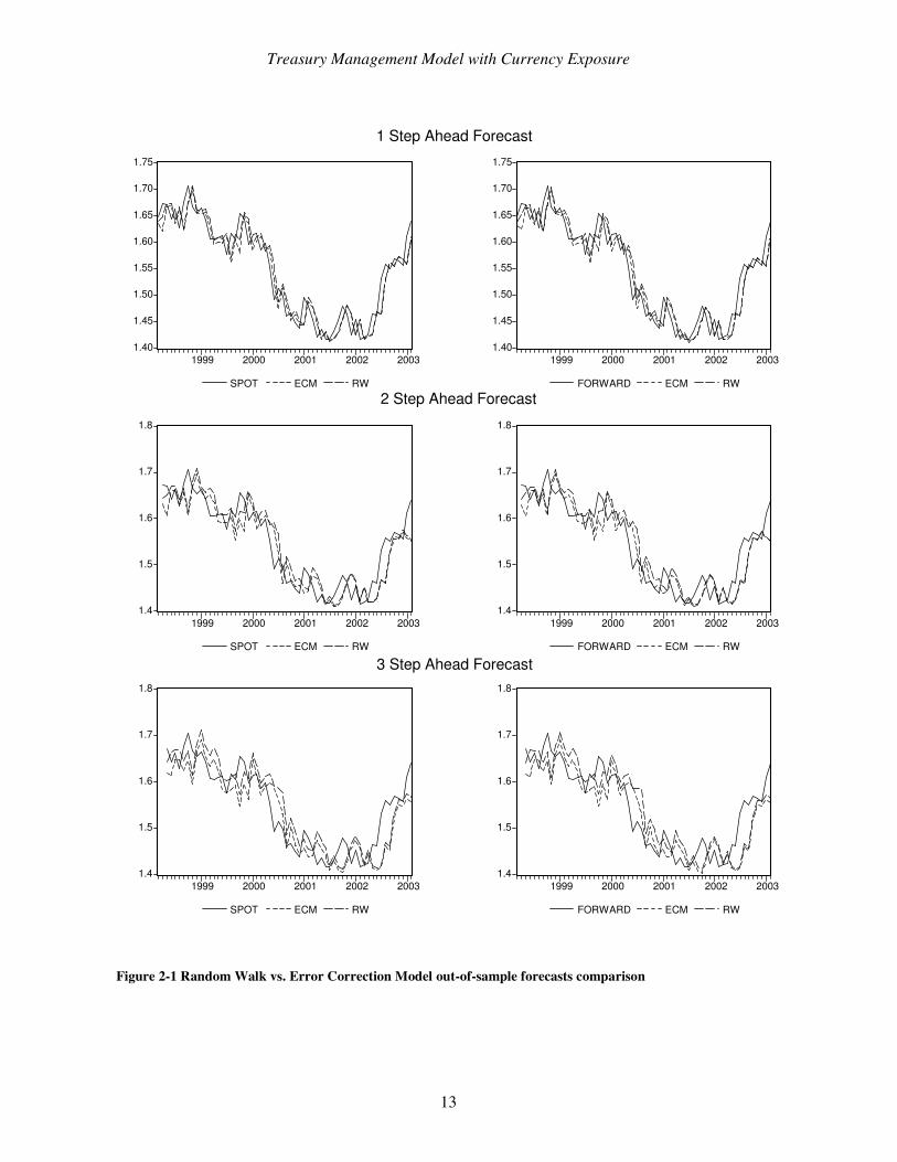
On the basis of the various criteria that are used to evaluate the forecast accuracy, the results are
clearly in favour of the VEC model specification. Therefore the VEC model is used for simulating

Treasury Management Model with Currency Exposure
12
scenarios of future exchange rates. Figure 2-1 demonstrates the one-, two- and three-step-ahead
out-of-sample forecasts of RW and ECM of exchange rates. The ECM follows more closely both
spot and forward exchange rates.
Treasury Management Model with Currency Exposure
13
1.40
1.45
1.50
1.55
1.60
1.65
1.70
1.75
1999 2000 2001 2002 2003
SPOT ECM RW
1.40
1.45
1.50
1.55
1.60
1.65
1.70
1.75
1999 2000 2001 2002 2003
FORWARD ECM RW
1.4
1.5
1.6
1.7
1.8
1999 2000 2001 2002 2003
SPOT ECM RW
1.4
1.5
1.6
1.7
1.8
1999 2000 2001 2002 2003
FORWARD ECM RW
1.4
1.5
1.6
1.7
1.8
1999 2000 2001 2002 2003
SPOT ECM RW
1.4
1.5
1.6
1.7
1.8
1999 2000 2001 2002 2003
FORWARD ECM RW
1 Step Ahead Forecast
2 Step Ahead Forecast
3 Step Ahead Forecast
Figure 2-1 Random Walk vs. Error Correction Model out-of-sample forecasts comparison
Treasury Management Model with Currency Exposure
14
2.3 Scenario Generation
The data set used in our empirical analysis consists of 241 observations of the spot and forward
(thirty-day rate) Sterling/Dollar exchange rate for the period from January 1984 to January 2004.
The spot and forward exchange rates were found to be integrated of order one and to cointegrate.4
This is in agreement with other studies.
Scenarios are generated using a series of recursive forecasts, which are computed in the following
way. For a given bivariate time series Ttttt sfw 1
'),( == a VEC model is fitted to the subseries
nTtttt sfw −== 1
'),( , where n is the desired number of forecasts and 12 is the longest forecast horizon
under consideration, and ',ttf and 'ts are the relevant forecasts.
Using nTt −= as the forecast origin, 100 sequences of t’-step-ahead forecasts are generated from
the fitted models for t’∈1,…,12, by drawing *tu randomly from the bivariate normal
distribution of tu . To ensure the relevance of our artificial time series, the values of the
parameters 22 , fs σσ and fs ,σ are chosen on the basis of the empirical variance-covariance matrix
obtained with the Sterling/Dollar exchange rate data.
The forecast origin is then rolled forward one period to 1+−= nTt , the parameters of the forecast
models are re-estimated and other 100 sequences of one-step-ahead to 12-step-ahead forecasts are
generated. The procedure is repeated until 100 forecasts are obtained for each t’∈1,…,12, which
are used as an input to the SP decision model.
2.4 The Scenario Tree
Consider a probability space, (,,)where Ω∈ω denotes parameter realisations with probability
Pp ∈)(ω and is a -field on . For the current time period t = 0: ',0 tf and s 0 are known with
certainty. Whereas, the data paths are depicted by the triplet ( )(),(),( '', ωωω psf ttt ), t = 1..T, t’ =
4 See note 2.
Treasury Management Model with Currency Exposure
15
1..T’, Ω= ..1ω , which provide all the necessary information about the forward and spot rates in the
future. In out model Ω
= 1)(ωp , that is, all the data paths are equiprobable.
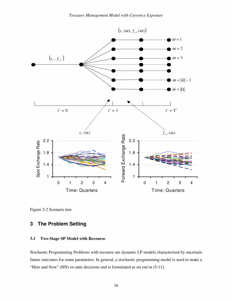
The model introduced in section 2.1 and validated in section 2.2 represents a stochastic process. For
the purpose of visualisation and a simple description, the behaviour of the parameters )(' ωts and
)(', ωttf over time, is illustrated by a tree of alternatives of possible parameter values with
corresponding probability weightings. Each expected path in this tree from the origin to the end of
the time horizon T’ is a “data path”. The scenario tree is illustrated in Figure 2-2.
Treasury Management Model with Currency Exposure
16
1
1.4
1.8
2.2
0 1 2 3 4
Time: Quarters
Forw
ard
Exc
hang
e R
ate
1
1.4
1.8
2.2
0 1 2 3 4
Time: Quarters
Spo
t Exc
hang
e R
ate
( ))(),( ',' ωω ttt fs
( )',', ttt fs
t’ = 0 t’ = 1 t’ = T’
1=ω
2=ω
3=ω
1−Ω=ω
Ω=ω
)(', ωttf)(' ωts
Figure 2-2 Scenario tree
3 The Problem Setting
3.1 Two Stage SP Model with Recourse
Stochastic Programming Problems with recourse are dynamic LP models characterised by uncertain
future outcomes for some parameters. In general, a stochastic programming model is used to make a
“Here and Now” (HN) ex-ante decisions and is formulated as set out in (5-11):
Treasury Management Model with Currency Exposure
17
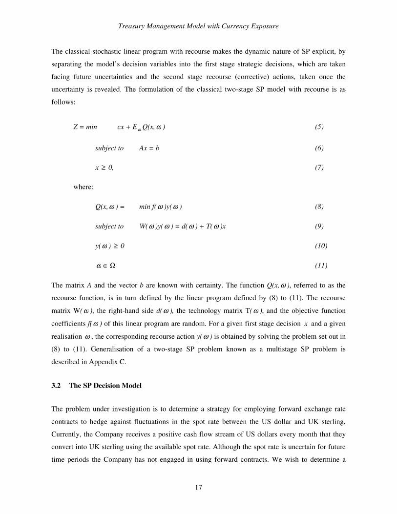
The classical stochastic linear program with recourse makes the dynamic nature of SP explicit, by
separating the model’s decision variables into the first stage strategic decisions, which are taken
facing future uncertainties and the second stage recourse (corrective) actions, taken once the
uncertainty is revealed. The formulation of the classical two-stage SP model with recourse is as
follows:
Z = min cx + E ω Q(x,ω ) (5)
subject to Ax = b (6)
x ≥ 0, (7)
where:
Q(x,ω ) = min f(ω )y(ω ) (8)
subject to W(ω )y(ω ) = d(ω ) + T(ω )x (9)
y(ω ) ≥ 0 (10)
ω ∈ Ω (11)
The matrix A and the vector b are known with certainty. The function Q(x,ω ), referred to as the
recourse function, is in turn defined by the linear program defined by (8) to (11). The recourse
matrix W(ω ), the right-hand side d(ω ), the technology matrix T(ω ), and the objective function
coefficients f(ω ) of this linear program are random. For a given first stage decision x and a given
realisation ω , the corresponding recourse action y(ω ) is obtained by solving the problem set out in
(8) to (11). Generalisation of a two-stage SP problem known as a multistage SP problem is
described in Appendix C.
3.2 The SP Decision Model
The problem under investigation is to determine a strategy for employing forward exchange rate
contracts to hedge against fluctuations in the spot rate between the US dollar and UK sterling.
Currently, the Company receives a positive cash flow stream of US dollars every month that they
convert into UK sterling using the available spot rate. Although the spot rate is uncertain for future
time periods the Company has not engaged in using forward contracts. We wish to determine a
Treasury Management Model with Currency Exposure
18
policy of hedging against such uncertainties by allowing the Company to engage in forward
contracts on exchange rates. Given the inherent risks in speculative trading in foreign exchange (see
Appendix B) we include limits to reduce the risks of speculation on forward exchange rates.
The uncertainties involving forward exchange rates have been modelled as a discrete set of
scenarios based on our work in VEC forecasting. We now develop a stochastic optimisation model
for determining the best “hedged” investments in forward contracts of exchange rates. The first
stage decisions represent the contracts on the forward exchange rates that should be purchased
while the second stage decisions are of two types: goal deviational variables and future decisions
about purchases of forward exchange rate contracts. We have adopted a similar approach to that of
Sharda and Wingender (1991). They formulate a goal-programming model to dynamically hedge
accounts receivables with futures currency contracts. We extend this method as follows:
Our objective function has three main components: (i) minimizing deviations from treasury targets,
similar to that of Sharda’s Goal Programming Model; (ii) minimizing transaction costs and (iii) we
maximise the company’s expected GBP-equivalent total income over the next 4 quarters. The
treasury manager specifies the weights attached to each of these main goals. In addition they also
set the level of risk exposure in achieving the third component of the objective.
By varying the weights assigned to different goals and varying the maximum forward exposure
limit, the treasury manager has the flexibility to choose their preferred strategy. The two-stage
stochastic programming decision model is formulated below.
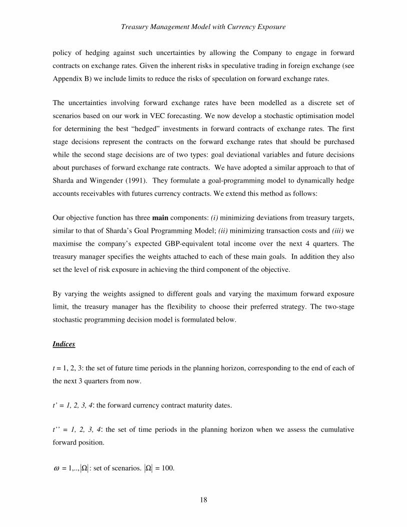
Indices
t = 1, 2, 3: the set of future time periods in the planning horizon, corresponding to the end of each of
the next 3 quarters from now.
t’ = 1, 2, 3, 4: the forward currency contract maturity dates.
t’’ = 1, 2, 3, 4: the set of time periods in the planning horizon when we assess the cumulative
forward position.
ω = 1,.., Ω : set of scenarios. Ω = 100.
Treasury Management Model with Currency Exposure
19
Data
Transaction cost:
TransCost: The transaction cost of acquiring / selling a forward currency contracts. Theoretically
there is no charge for entering a forward agreement though the bank could charge for selling back
the outstanding forward contract (closing out a forward position). Transaction cost can also reflect
an ask-bid spread. In this study we set the value of transaction costs at 0.1% of the contract value.
Exchange rates:
USDFwdRateCurrent 't : Currently available forward exchange rate on selling USD with maturity t’.
USDFwdRateFuture ',, ttω : Forecasted forward exchange rate on selling (buying) USD at time t with
maturity t’ under scenario ω , for ω ∈ Ω , t ∈ [1, 2, 3], t’ ∈ [2, 3, 4] and t’ > t.
USDSpotRate ',tω : Forecasted spot exchange rate on selling USD at a future time t’ under scenario
ω , for ω ∈ Ω , t’ ∈ [1, 2, 3, 4].
USDSpotRateCurrent: Current spot exchange rate on selling USD for GBP.
Cash Flows:
NetCashFlow 't : Amount of USD revenue less expenses in month t’, for t’ ∈ [1, 2, 3, 4].
Initial data:
FwdPrev 't : Number of forward currency contracts brought forward from the previous quarter with
maturity month t’, for t’ ∈ [1, 2, 3].
Other data:
Treasury Management Model with Currency Exposure
20
UpperLimitOnHedge: Treasury set upper limit on the proportion of the net cash flows to be offset
by taking a position in the forward exchange rate contracts.
ωobPr : Probability of scenario ω .
1W 2W and 3W : The weights assigned to the three main components of the objective.
w 1,1 , w 2,1 , w 3,1 : The weights assigned to the 1-st, the 2-nd and the 3-rd goal associated with
deviation from treasury targets.
First-Stage Decision Variables
XFwdHoldt’: The total amount of current USD forward currency contracts held with maturity date
t’, for t’ ∈ [1, 2, 3, 4].
XFwdBuyt’: The number of forward currency contracts acquired at the beginning of the current
month with maturity date t’, for t’ ∈ [1, 2, 3, 4].
XFwdSellt’: The number of forward currency contracts settled (sold) at the beginning of the current
month with maturity t’, for t’ ∈ [1, 2, 3, 4].
Second-Stage Variables
YFwdBuy ',, ttω : The amount of USD to buy forward at the beginning of month t with maturity date t’
under scenario ω where t < t’, for ω ∈ Ω , t ∈ [1, 2, 3], t’∈ [2, 3, 4].
YFwdSell ',, ttω : The expected amount of USD to sell forward at the beginning of month t with
maturity date t’ under scenario ω where t < t’, for ω ∈ Ω , t ∈ [1, 2, 3], t’∈ [2, 3, 4].
ExpectedGBPValFromSpot: A reporting variable representing the expected GBP-converted
income from future net cash flows for quarters: 1, 2, 3 and 4 using spot exchange rates at the same
time as when the income stream is received.
Treasury Management Model with Currency Exposure
21
ExpectedGBPValFromForward: The expected GBP-converted income e.g. gain or loss, from the
positions taken in forward currency contracts made over the next 4 quarters.
ExpTransCost: The expected transaction costs for the positions taken in forward currency contracts
over the next 4 quarters.
UnderHedge ',tω : A goal variable representing the GBP amount by which the change in cash flows
with maturity t’ is larger than the change in forward currency position for quarter t’ under scenario
ω , for ω ∈ Ω , t’ ∈ [1, 2, 3, 4].
OverHedge ',tω : A goal variable representing the GBP amount by which the change in cash flows
with maturity t’ is less than the change in forward currency position for quarter t’ under scenario ω ,
for ω ∈ Ω , t’ ∈ [1, 2, 3, 4].
TopUp ',tω : A goal variable representing the speculative loss, i.e. the amount of GBP top-up to the
“virtual margin account” during quarter t’ under scenario ω , for ω ∈ Ω , t’ ∈ [1, 2, 3, 4].
Objective Function
The objective function represents a trade-off between the immediate potential losses in the first
quarter, the expected transaction costs and the value of the wealth over the whole planning horizon.
These are now described.
Goal 1: Deviations from the treasury targets (imminent losses).
By assigning different (respective) weights and summing into a linear form this goal is decomposed
into three sub-goals summarized below.
1.1 Minimize the expected change in the cash flow over the change in the forward position.
1.2 Minimize the expected change in the forward currency position over the change in the cash
flows.
1.3 Minimize the expected top-up amount on the “virtual margin account” i.e. speculative loss.
Treasury Management Model with Currency Exposure
22
Goal 2: Minimize expected transaction costs over the next four quarters
Goal 3: Maximize expected cumulative GBP-equivalent income over the next four quarters
This goal is achieved by maximizing the two sub-goals shown below:
Future net cash flows over t’, where t’ ∈ [1, 2, 3, 4], converted to GBP at the spot exchange rates at
the time income is received.
Expected cumulative GBP-equivalent gain or loss made over t’, where t’ ∈ [1, 2, 3, 4] from taking
positions in forward exchange rate contracts.
The algebraic representation of the complete objective function is as follows:
Min Z = W 1 * (w 1,1 * Ω∈ =ω
ωω
'
1'',*Pr
T
ttUnderHedgeob
+ w 2,1 * Ω∈ =ω
ωω
'
1'',*Pr
T
ttOverHedgeob
+ w 3,1 * Ω∈ =ω
ωω
'
1'',*Pr
T
ttTopUpob )
+ stExpTransCoW *2
- 3W * (ExpectedGBPValFromSpot +ExpectedGBPValFromForward) (12)
subject to:
1) Constraints related to treasury target
Treasury Management Model with Currency Exposure
23
XFwdHold 1 (1/USDFwdRateCurrent 1 - 1/USDSpotRate 1,ω ) + UnderHedge 1,ω -
OverHedge 1,ω = NetCashFlow 1,ω (1/USDSpotRateCurrent –1/USDSpotRate 1,ω )
ω∀
(13)
Equation (13) seeks to establish the necessary forward position for maturity t’ = 1 in order to offset
the changes in the net cash flows in three months time. The UnderHedge 1,ω and OverHedge 1,ω
represent under and over achievements of this goal. Although the model is developed over four
(quarters) time periods, we are more concerned with potential losses in the next quarter. This
constraint emphasises that this can be hedged against by committing to more forward contracts.
XFwdHold 't (1/USDFwdRateCurrent 't - 1/USDFwdRateFuture ',1, tω ) +
UnderHedge ',tω - OverHedge ',tω = NetCashFlow ',tω (1/USDSpotRateCurrent -
1/USDSpotRate 1,ω ) ω∀ , t’ > 1
(14)
Equation (14) similarly considers the same issues as for equation (13) but for contracts with
maturities t’> 1. The UnderHedge ',tω and OverHedge ',tω represent under and over achievements of
this goal.
XFwdHold 1 (1/ USDFwdRateCurrent1 - 1/ USDSpotRate 1,ω ) + TopUp 1,ω ≥ 0
ω∀
(15)
Equations (13) and (14) encourage investing in forward contracts, while constraint (15) accounts for
possible losses incurred in these forward contracts and as such, conflicts with constraint (13). By
changing the weights in the objective of these deviational variables it is possible to investigate
different strategies for controlling speculation in the forward market.
XFwdHold 't (1/ USDFwdRateCurrent 't -1/ USDFwdRateFuture ',1, tω ) + TopUp ',tω ≥ 0
ω∀ , t’ > 1
(16)
Treasury Management Model with Currency Exposure
24
Similarly, the set of equations (16) account for losses in forward contracts maturing in later time
periods.
2) Expected Transaction Cost Constraint
=
+='
1''' )(*
T
ttt XFwdSellXFwdBuyTransCoststExpTransCo
)(*Pr* ',,
1'
1
'
1'',, tt
t
t
T
ttt YFwdSellYFwdBuyobTransCost ωω
ωω ++
−
= =Ω∈ (17)
Equation (17) measures the expected transaction costs for the next 4 quarters from purchasing
(selling) forward currency contracts.
3) Constraints related to the final wealth objective
The following constraints are all related to measuring the final wealth of the revenues converted to
sterling. The first set of constraints are balance constraints for forward contracts with maturity t’
quarters ahead
XFwdHold 't = FwdPrev 't + XFwdBuy 't - XFwdSell 't 't∀ (18)
Equation (18) represents a balance constraint on the activities with forward exchange rate contracts,
which actually take place at the beginning of the current time period.
XFwdHold 't + =
''
1
t
t
(YFwdBuy ',, ttω - YFwdSell ',, ttω )
≤ UpperLimitOnHedge * NetCashFlow ',tω ω∀ , 1'>t , 1'..1'' −= tt
(19)
Equations (19) represent an upper limit on the expected cumulative forward exchange rate position
at any future time period t’’.
Treasury Management Model with Currency Exposure
25
XFwdHold 't + =
''
1
t
t
(YFwdBuy ',, ttω - YFwdSell ',, ttω ) ≥ 0
ω∀ , 1'>t , 1'..1'' −= tt
(20)
Equation (20) states that no short sales are allowed on forward contracts.
YFwdBuy ',, ttω + YFwdSell ',, ttω ≤ UpperLimitOnHedge * NetCashFlow ',tω
ω∀ , 1'>t , 1'..1 −= tt
(21)
Equation (21) defines the upper limit on the future expected forward exchange rate trades.
XFwdHold 't ≤ UpperLimitOnHedge * NetCashFlow ',tω ω∀ , 1'>t (22)
Equation (22) represents an upper limit on the actual forward exchange rate position opened during
the current time period.
',
'
1'', /*Pr t
T
tt eUSDSpotRatwNetCashFloobotPValFromSpExpectedGB ωω
ωω
=Ω∈
= (23)
Equation (23) reports the expected GBP-valued cumulative net cash flows for the 4 quarters using
spot exchange rates at the time when the cash flow is received.
=rwardPValFromFoExpectedGB
)/1/1(*Pr ',
'
1''' t
T
ttt eUSDSpotRatCurrentUSDFwdRateXFwdHoldob ω
ωω
=Ω∈
−
+ Ω∈
<
−
= =
−ω
ωωωω ',',',,
1'
1
'
1'',, 1)((*Pr ttttt
t
t
T
ttt FutureUSDFwdRateYFwdSellYFwdBuyob
)1 ',teUSDSpotRat ω− (24)
Treasury Management Model with Currency Exposure
26
Equation (24) measures the expected marginal benefit from using forward currency contracts for the
planning horizon, e.g. the company either obtains a speculative gain or a loss from entering forward
currency contracts with various maturities.
4 Backtesting and Rolling forward the SP Decision Model
Our modelling framework has three aspects (a) calibration of the VECM model, which is used for
scenario generation, (b) a decision model, (c) a simulation model to evaluate the decisions
(backtesting). In our case there are three decision models, namely, Here-and-Now (HN), Expected
Value (EV) and Perfect Information (PI) models (see section 4.3). For the purpose of simulation
and backtesting we split the historical data into two parts. The Part 1 comprises first 169 monthly
observations (Jan. 1984 to Jan. 1998) and the Part 2 comprises 60 months (Feb. 1998 to Jan. 2003)
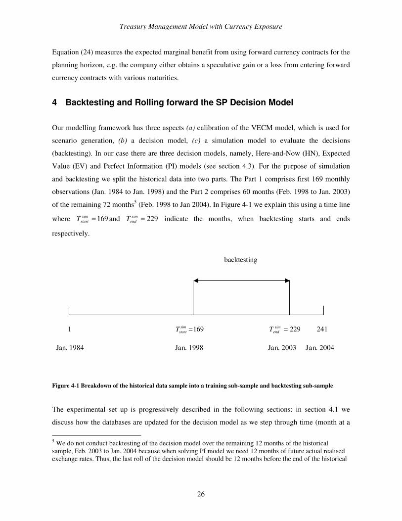
of the remaining 72 months5 (Feb. 1998 to Jan 2004). In Figure 4-1 we explain this using a time line
where 169=simstartT and 229=sim
endT indicate the months, when backtesting starts and ends
respectively.
1 169=simstartT 229=sim
endT 241
backtesting
Jan. 1984 Jan. 1998 Jan. 2003 Jan. 2004
Figure 4-1 Breakdown of the historical data sample into a training sub-sample and backtesting sub-sample
The experimental set up is progressively described in the following sections: in section 4.1 we
discuss how the databases are updated for the decision model as we step through time (month at a
5 We do not conduct backtesting of the decision model over the remaining 12 months of the historical sample, Feb. 2003 to Jan. 2004 because when solving PI model we need 12 months of future actual realised exchange rates. Thus, the last roll of the decision model should be 12 months before the end of the historical
Treasury Management Model with Currency Exposure
27
time), section 4.2 explains the rolling of the decision model, then in section 4.3 we contrast three
different decision models on the basis of Risk and Return (Income) and in section 4.4 we compare
different treasury strategies on the basis of stochastic measures.
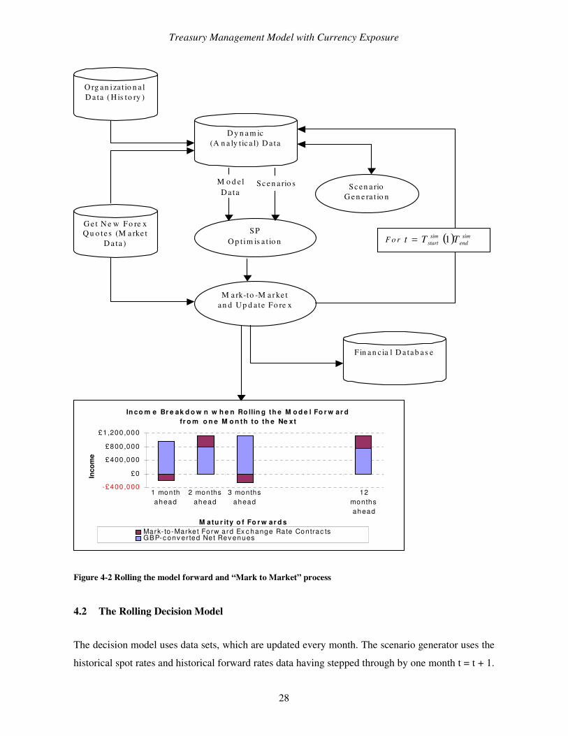
4.1 Dynamic Data Model
The role of the historical market data, the organisational data, their interaction with the decision
model and backtesting are illustrated in Figure 4-2. The experimental set up requires that we
dynamically:
(i) Use market data in order to revalue the forward positions, a well-known “mark to market”
procedure.
(ii) We also record the decisions made in the current step of the model as an input of the
starting position of the next “roll” of the model.
Whereas in futures currency contracts there is an external requirement for “marking to market”, for
forward positions there is no such obligation. As an “internal good practice procedure”, however,
we have introduced this in our “Forward currency contract” decision model so that we are able to
compute the “moneyness” of the current positions to give some indication of ongoing performances.
Thus for each time movement the model database is updated with the most currently available
forward rates and spot rates. By accessing our current forward commitments along with their
current marked to market forward rate from the model database, we adjust our forward rates to be
the same as the current month forward rates. The process of “marking to market” of our currently
held forward contracts involves realigning the contracts by one time period as well as determining
the financial losses or gains made on our forward positions. Similarly, we close out the opening
income stream using a combination of currently maturing forward contracts and the current spot
rate. All these cash transactions, namely the marking to market of forwards contracts and
conversion of the current income revenue are recorded in our financial database.
sample of exchange rates. In order to compare PI model with HN and EV models on like-for-like bases we use the same backtesting time period for all the models.
Treasury Management Model with Currency Exposure
28
D y n a m ic (A n a ly tic a l) D a ta
Sc en a rio G e n e ra t io n
SP O p t im is a t io n
M a rk-to -M a r ke t an d Up d a te Fo re x
F in a n c ia l D a tab a s e
In co m e Br e ak d o w n w h e n Ro llin g th e M o d e l Fo r w ar d fr o m o n e M o n th to th e Ne xt
-£400,000
£0
£400,000
£800,000
£1,200,000
1 monthahead
2 monthsahead
3 monthsahead
12monthsahead
M atu r ity o f Fo r w ar d s
Inco
me
Mark- to -Marke t Forw ard Ex c hange Rate Contrac tsGBP-c onv er ted Net Rev enues
G e t N e w Fo re x Q u o te s (M a rke t
D a ta )
O rg an iza t io n a l D a ta ( H is to ry )
M o d e l Da ta
Sc e n a rio s
F o r ( ) simend
simstart TTt 1=
Figure 4-2 Rolling the model forward and “Mark to Market” process
4.2 The Rolling Decision Model
The decision model uses data sets, which are updated every month. The scenario generator uses the
historical spot rates and historical forward rates data having stepped through by one month t = t + 1.
Treasury Management Model with Currency Exposure
29
Thus the scenario generator creates a completely new set of scenarios looking ahead over a time
horizon of T = 12 months. In respect of revenues we have developed a scenario generator for
representing alternative realisations of the future income but in our current analyses we have
assumed that the income stream remains constant.
Given that the decisions are made altogether 60 times by stepping through the time line
( ) simend
simstart TTt 1= we process the corresponding TWOSP model 60 times using the SPInE system. The
SPInE system has the dual capability of SP decision modelling and simulation (see Valente et al
2004, and Di Domenica et al 2004).
The figure 4-2 also illustrates the results produced by the rolling model. The accompanying plot
illustrates the effects of marking to market, which may have two outcomes. Firstly, in realigning our
forward contracts to the current rates we either make some profit on our currently held forward
contracts or our speculation has led to a loss, these are represented by the red bars. Secondly, in
processing the current month’s revenue we use the spot rate thus the income revenue is marked to
market and is represented by the blue bars.
4.3 Simulation 1: Risk and Return Analysis
In this paper we estimate risk exposure of each treasury strategy by calculating Value-at-Risk (VaR)
measure. A brief description of some other commonly used risk measure is provided in Appendix
A. The meaning of VaR in our paper is slightly different from the conventional one. When dealing
with returns on investments VaR represents the maximum loss incurred with certain probability
(e.g. 95%). In our case, since we are dealing with revenues, not returns, VaR represents the lowest
monthly revenue achieved with certain probability. As a result, in the case of returns one aims at a
smaller VaR, i.e. smaller loss but in our case we are better off having larger VaR, i.e. larger
monthly revenues at a certain probability level.
We have assumed constant revenue throughout the planning horizon, also the financial decisions
made prior to each optimisation run are independent; we run the rolling decision model and create a
histogram with appropriate bins and compute VaR values for different probability levels for the
monthly income.
Treasury Management Model with Currency Exposure
30
In order to evaluate the impact of randomness on (optimal) decision we backtest the three rolling
models over 60 months of the historical sample, Feb. 1998 to Jan. 2003.
• Here-and-Now (HN): represents the TWOSP model described in section 3.1.
• Expected Value (EV): is the deterministic representation of our treasury model for foreign
exchange rate exposure with the uncertain parameters replaced with by their expected
values.
• Perfect Information (PI): is the deterministic representation of our treasury model for foreign
exchange rate exposure with the true realised data for the uncertain parameters (historical
data as scenarios). This model is the true upper bound on the overall optimisation problem.
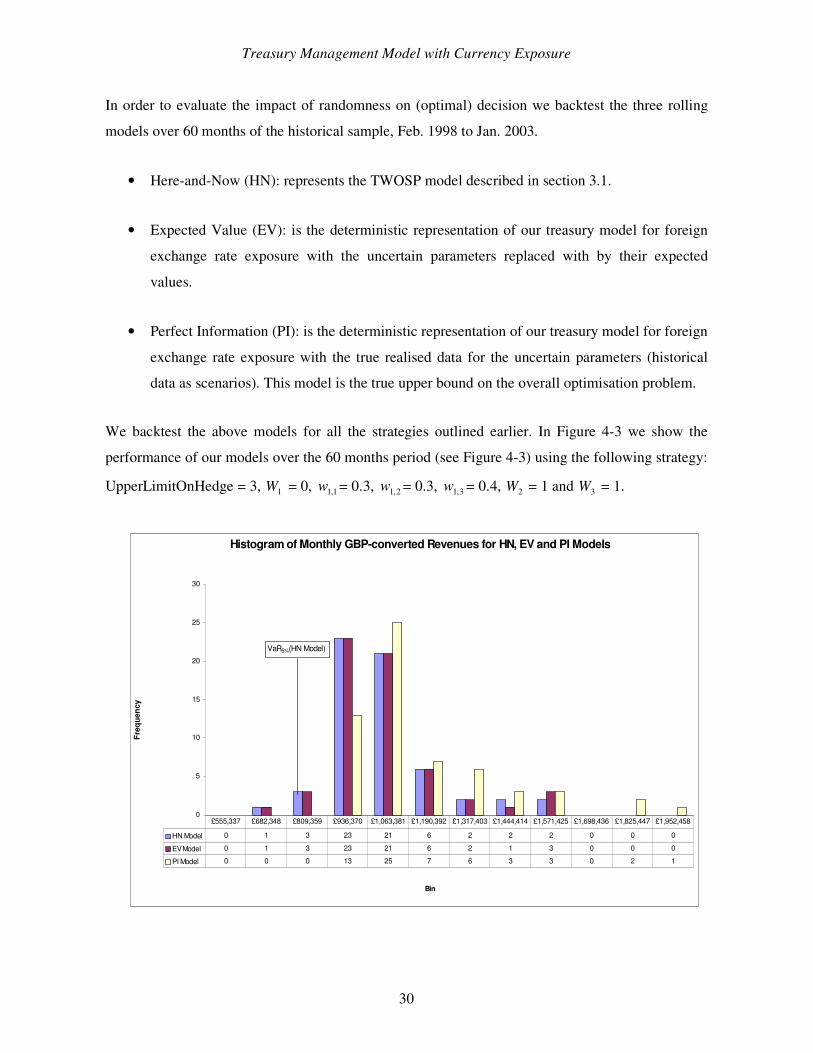
We backtest the above models for all the strategies outlined earlier. In Figure 4-3 we show the
performance of our models over the 60 months period (see Figure 4-3) using the following strategy:
UpperLimitOnHedge = 3, 1W = 0, 1,1w = 0.3, 2,1w = 0.3, 3,1w = 0.4, 2W = 1 and 3W = 1.
Histogram of Monthly GBP-converted Revenues for HN, EV and PI Models
0
5
10
15
20
25
30
Bin
Freq
uenc
y
HN Model 0 1 3 23 21 6 2 2 2 0 0 0
EV Model 0 1 3 23 21 6 2 1 3 0 0 0
PI Model 0 0 0 13 25 7 6 3 3 0 2 1
£555,337 £682,348 £809,359 £936,370 £1,063,381 £1,190,392 £1,317,403 £1,444,414 £1,571,425 £1,698,436 £1,825,447 £1,952,458
VaR5%(HN Model)
Treasury Management Model with Currency Exposure
31
Figure 4-3 Histograms of monthly revenues associated with the output of each of the 3 models (HN, EV, PI), backtested to identify the revenue that those models (decisions) would have yielded
Figure 4-3 shows that the EV model has a marginally longer right tail than that of the HN model. It
also shows that for this strategy the distribution for the EV decision is preferable to that of HN.
However, if we consider a range of strategies as in Table 4-1 we see that this is not always the case.
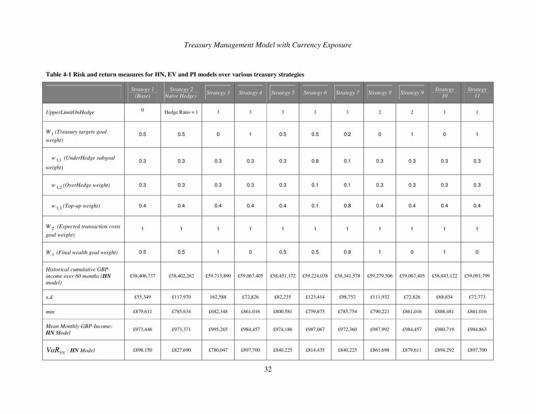
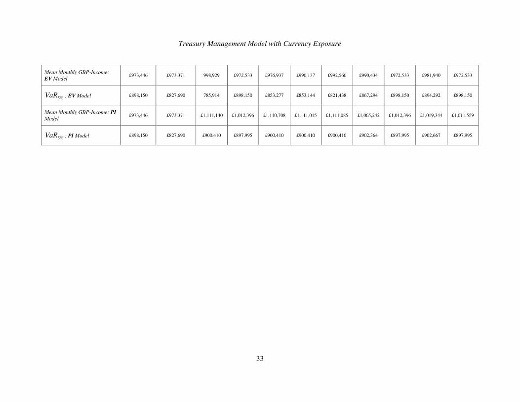
Table 4-1 summarises the risk and returns measures for the 3 models investigated: PI, HN and EV
over various treasury strategies. Each simulation run provides a possible realisation of the financial
income received for any given time period. Experiments have been carried out on a number of
different strategies each representing a particular upper limit on the forward exchange rate position
and a combination of different penalties for not meeting the treasury targets.
Treasury Management Model with Currency Exposure
32
Table 4-1 Risk and return measures for HN, EV and PI models over various treasury strategies
Strategy 1 (Base)
Strategy 2 (Naïve Hedge) Strategy 3 Strategy 4 Strategy 5 Strategy 6 Strategy 7 Strategy 8 Strategy 9 Strategy
10 Strategy
11
UpperLimitOnHedge 0 Hedge Ratio = 1 3 3 3 3 3 2 2 1 1
W 1 (Treasury targets goal weight)
0.5 0.5 0 1 0.5 0.5 0.2 0 1 0 1
w 1,1 (UnderHedge subgoal
weight) 0.3 0.3 0.3 0.3 0.3 0.8 0.1 0.3 0.3 0.3 0.3
w 2,1 (OverHedge weight) 0.3 0.3 0.3 0.3 0.3 0.1 0.1 0.3 0.3 0.3 0.3
w 3,1 (Top-up weight) 0.4 0.4 0.4 0.4 0.4 0.1 0.8 0.4 0.4 0.4 0.4
W 2 (Expected transaction costs goal weight)
1 1 1 1 1 1 1 1 1 1 1
W 3 (Final wealth goal weight) 0.5 0.5 1 0 0.5 0.5 0.8 1 0 1 0
Historical cumulative GBP-income over 60 months (HN model)
£58,406,737 £58,402,262 £59,715,890 £59,067,405 £58,451,172 £59,224,038 £58,341,578 £59,279,506 £59,067,405 £58,843,122 £59,091,799
s.d. £55,349 £117,970 162,588 £72,826 £82,235 £123,414 £98,752 £111,932 £72,826 £68,834 £72,773
min £879,611 £785,634 £682,348 £861,016 £800,581 £759,875 £785,754 £790,221 £861,016 £888,481 £861,016
Mean Monthly GBP-Income: HN Model
£973,446 £973,371 £995,265 £984,457 £974,186 £987,067 £972,360 £987,992 £984,457 £980,719 £984,863
%5VaR : HN Model £898,150 £827,690 £780,047 £897,700 £840,225 £814,435 £840,225 £861,698 £879,611 £894,292 £897,700
Treasury Management Model with Currency Exposure
33
Mean Monthly GBP-Income: EV Model
£973,446 £973,371 998,929 £972,533 £976,937 £990,137 £992,560 £990,434 £972,533 £981,940 £972,533
%5VaR : EV Model £898,150 £827,690 785,914 £898,150 £853,277 £853,144 £821,438 £867,294 £898,150 £894,292 £898,150
Mean Monthly GBP-Income: PI Model
£973,446 £973,371 £1,111,140 £1,012,396 £1,110,708 £1,111,015 £1,111,085 £1,065,242 £1,012,396 £1,019,344 £1,011,559
%5VaR : PI Model £898,150 £827,690 £900,410 £897,995 £900,410 £900,410 £900,410 £902,364 £897,995 £902,667 £897,995
Treasury Management Model with Currency Exposure
34
As we can see from the above table, %5VaR there is a trade-off between VaR and Revenues.
Surprisingly, EV Model did not do worse that HN Model, which reflects the quality of the scenario
generator. At the same time if we could “perfectly” foresee the future realisations of exchange rates
we would receive higher monthly revenues. This also shows the potential for achieving better
results by improving scenario generation model.
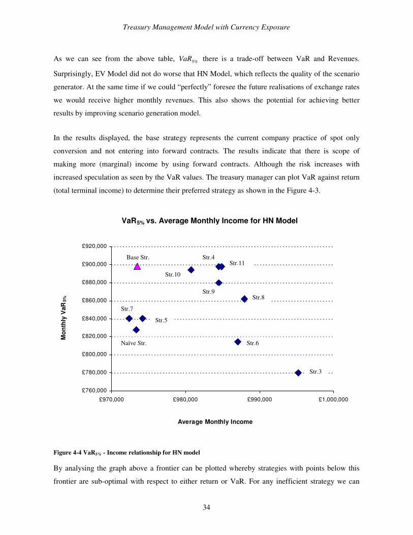
In the results displayed, the base strategy represents the current company practice of spot only
conversion and not entering into forward contracts. The results indicate that there is scope of
making more (marginal) income by using forward contracts. Although the risk increases with
increased speculation as seen by the VaR values. The treasury manager can plot VaR against return
(total terminal income) to determine their preferred strategy as shown in the Figure 4-3.
VaR5% vs. Average Monthly Income for HN Model
£760,000
£780,000
£800,000
£820,000
£840,000
£860,000
£880,000
£900,000
£920,000
£970,000 £980,000 £990,000 £1,000,000
Average Monthly Income
Mon
thly
VaR
5%
Figure 4-4 VaR5% - Income relationship for HN model
By analysing the graph above a frontier can be plotted whereby strategies with points below this
frontier are sub-optimal with respect to either return or VaR. For any inefficient strategy we can
Base Str.
Str.10
Str.4Str.11
Str.9Str.8
Str.6
Str.3
Str.5
Str.7
Naïve Str.
Treasury Management Model with Currency Exposure
35
find an efficient point with more return for this level of VaR, or higher VaR for this given level of
return. Our current investigations are looking at how easy it is to determine the various strategies to
create points on the “efficient” frontier.
4.4 Simulation 2: Stochastic Measures
In SP models the expected value of perfect information (EVPI) indicates, how far the stochasticity
impinges on the decision-making. EEV stands for the expectation of the expected value (EEV)
problem The methods of computing these measures are summarised in Appendix C. For a full
discussion of stochastic measures including EVPI and EEV we refer the reader to Birge and
Louveaux [1997], p.138-142.
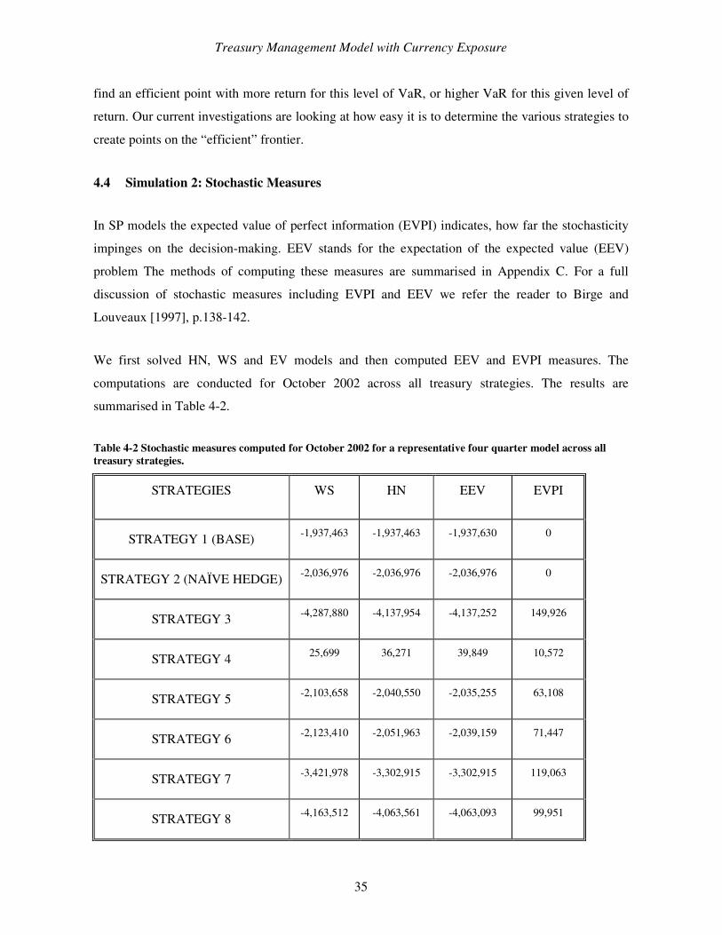
We first solved HN, WS and EV models and then computed EEV and EVPI measures. The
computations are conducted for October 2002 across all treasury strategies. The results are
summarised in Table 4-2.
Table 4-2 Stochastic measures computed for October 2002 for a representative four quarter model across all treasury strategies.
STRATEGIES WS HN EEV EVPI
STRATEGY 1 (BASE) -1,937,463 -1,937,463 -1,937,630 0
STRATEGY 2 (NAÏVE HEDGE) -2,036,976 -2,036,976 -2,036,976 0
STRATEGY 3 -4,287,880 -4,137,954 -4,137,252 149,926
STRATEGY 4 25,699 36,271 39,849 10,572
STRATEGY 5 -2,103,658 -2,040,550 -2,035,255 63,108
STRATEGY 6 -2,123,410 -2,051,963 -2,039,159 71,447
STRATEGY 7 -3,421,978 -3,302,915 -3,302,915 119,063
STRATEGY 8 -4,163,512 -4,063,561 -4,063,093 99,951
Treasury Management Model with Currency Exposure
36
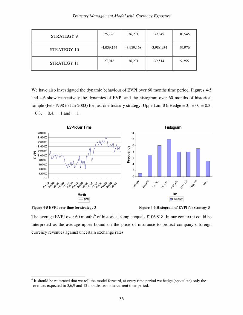
STRATEGY 9 25,726 36,271 39,849 10,545
STRATEGY 10 -4,039,144 -3,989,168 -3,988,934 49,976
STRATEGY 11 27,016 36,271 39,514 9,255
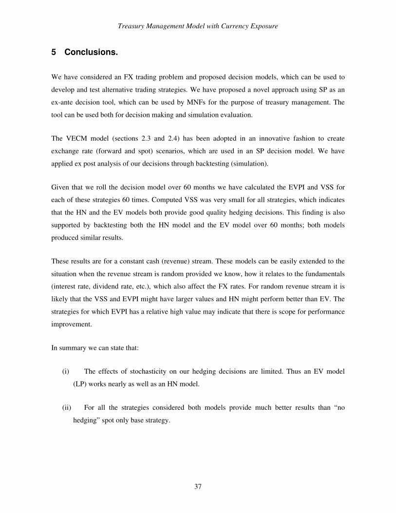
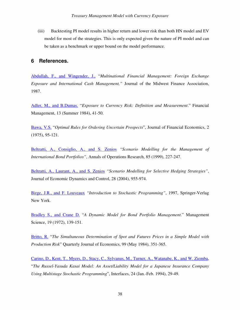
We have also investigated the dynamic behaviour of EVPI over 60 months time period. Figures 4-5
and 4-6 show respectively the dynamics of EVPI and the histogram over 60 months of historical
sample (Feb-1998 to Jan-2003) for just one treasury strategy: UpperLimitOnHedge = 3, = 0, = 0.3,
= 0.3, = 0.4, = 1 and = 1.
EVPI over Time
£0
£20,000
£40,000
£60,000
£80,000
£100,000
£120,000
£140,000
£160,000
£180,000
£200,000
Feb-9
8
Jun-9
8
Oct-98
Feb-9
9
Jun-9
9
Oct-99Fe
b-00
Jun-0
0
Oct-00Fe
b-01
Jun-0
1
Oct-01Fe
b-02
Jun-0
2
Oct-02
Month
EV
PI
EVPI
Histogram
0
2
4
6
8
10
12
14
More
Bin
Freq
uenc
y
Frequency
Figure 4-5 EVPI over time for strategy 3 Figure 4-6 Histogram of EVPI for strategy 3
The average EVPI over 60 months6 of historical sample equals £106,818. In our context it could be
interpreted as the average upper bound on the price of insurance to protect company’s foreign
currency revenues against uncertain exchange rates.
6 It should be reiterated that we roll the model forward, at every time period we hedge (speculate) only the revenues expected in 3,6,9 and 12 months from the current time period.
Treasury Management Model with Currency Exposure
37
5 Conclusions.
We have considered an FX trading problem and proposed decision models, which can be used to
develop and test alternative trading strategies. We have proposed a novel approach using SP as an
ex-ante decision tool, which can be used by MNFs for the purpose of treasury management. The
tool can be used both for decision making and simulation evaluation.
The VECM model (sections 2.3 and 2.4) has been adopted in an innovative fashion to create
exchange rate (forward and spot) scenarios, which are used in an SP decision model. We have
applied ex post analysis of our decisions through backtesting (simulation).
Given that we roll the decision model over 60 months we have calculated the EVPI and VSS for
each of these strategies 60 times. Computed VSS was very small for all strategies, which indicates
that the HN and the EV models both provide good quality hedging decisions. This finding is also
supported by backtesting both the HN model and the EV model over 60 months; both models
produced similar results.
These results are for a constant cash (revenue) stream. These models can be easily extended to the
situation when the revenue stream is random provided we know, how it relates to the fundamentals
(interest rate, dividend rate, etc.), which also affect the FX rates. For random revenue stream it is
likely that the VSS and EVPI might have larger values and HN might perform better than EV. The
strategies for which EVPI has a relative high value may indicate that there is scope for performance
improvement.
In summary we can state that:
(i) The effects of stochasticity on our hedging decisions are limited. Thus an EV model
(LP) works nearly as well as an HN model.
(ii) For all the strategies considered both models provide much better results than “no
hedging” spot only base strategy.
Treasury Management Model with Currency Exposure
38
(iii) Backtesting PI model results in higher return and lower risk than both HN model and EV
model for most of the strategies. This is only expected given the nature of PI model and can
be taken as a benchmark or upper bound on the model performance.
6 References.
Abdullah, F., and Wingender, J., “Multinational Financial Management: Foreign Exchange
Exposure and International Cash Management,” Journal of the Midwest Finance Association,
1987.
Adler, M., and B.Dumas. “Exposure to Currency Risk: Definition and Measurement.” Financial
Management, 13 (Summer 1984), 41-50.
Bawa, V.S. “Optimal Rules for Ordering Uncertain Prospects”, Journal of Financial Economics, 2
(1975), 95-121.
Beltratti, A., Consiglio, A., and S. Zenios “Scenario Modelling for the Management of
International Bond Portfolios”, Annals of Operations Research, 85 (1999), 227-247.
Beltratti, A., Laurant, A., and S. Zenios “Scenario Modelling for Selective Hedging Strategies”,
Journal of Economic Dynamics and Control, 28 (2004), 955-974.
Birge, J.R., and F. Louveaux “Introduction to Stochastic Programming”, 1997, Springer-Verlag
New York.
Bradley S., and Crane D. “A Dynamic Model for Bond Portfolio Management.” Management
Science, 19 (1972), 139-151.
Britto, R. “The Simultaneous Determination of Spot and Futures Prices in a Simple Model with
Production Risk” Quarterly Journal of Economics, 99 (May 1984), 351-365.
Carino, D., Kent, T., Myers, D., Stacy, C., Sylvanus, M., Turner, A., Watanabe, K., and W. Ziemba,
“The Russel-Yasuda Kasai Model: An Asset/Liability Model for a Japanese Insurance Company
Using Multistage Stochastic Programming”, Interfaces, 24 (Jan.-Feb. 1994), 29-49.
Treasury Management Model with Currency Exposure
39
Diebold, F.X., and R.S. Mariano “Comparing Predictive Accuracy”, Journal of Business and
Economic Statistics, 13 (1995), 253-263.
Di Domenica N., Birbilis B., Mitra G., and P. Valente “Stochastic Programming and Scenario
Generation within a Simulation Framework : An Information Systems Perspective”, Technical
Report No (2004), Centre for the Analysis of Risk and Optimisation Modelling Applications
(CARISMA)
Dumas, B. “Short- and Long-term Hedging for the Corporation”, Discussion Paper No. 1083
(1994), Centre for Economic Policy Research, www.cepr.org/pubs/dps/DP1083.asp.
Eaker, M. R., and D. Grant. “Optimal Hedging of Uncertain and Long-term Foreign Exchange
Exposure.” Journal of Banking and Finance, 9 (June 1985), 221-231.
Ederington, L. “The Hedging Performance of the New Futures Markets.” The Journal of Finance,
Vol. 34 (Mar., 1979), 157-170.
Engle R.F., and C.W.J. Granger “Cointegration and Error-Correction: Representation, Estimation,
and Testing.” Econometrica, 55 (March 1987), 251-76.
Fishburn, P.C. “Mean-Risk Analysis with Risk Associated with Below-Target Returns”, American
Economic Review, 67 (1977), 116-126.
Golub, B., Holmer, M., McKendall, R., Pohlman, L., and S. Zenios, “A Stochastic Programming
Model for Money Management.” European Journal of Operational Research, 85 (1995), 282-296.
Granger, C.W.J. “Some Properties of Time Series Data and Their Use in Econometric Model
Specifications.” Journal of Econometrics, 16 (1981), 121-130
Granger, C.W.J. “ Co-integrated Variables and Error Correcting Models”, Discussion Paper No.
83-13a, (1983), University of California, San Diego.
Hirschleifer, D. “Risk, Futures Pricing, and the Organization of Production in Commodity
Markets.” Journal of Political Economy, 96 (Dec. 1988), 1206-1220.
Treasury Management Model with Currency Exposure
40
Kerkvliet, J., and M.H.Moffett “The Hedging of an Uncertain Future Foreign Currency Cash
Flow.” The Journal of Financial and Quantitative Analysis, Vol. 26 (Dec. 1991), 565-578.
Klaassen, P., Shapiro J.F., and D.E. Spitz “Sequential Decision Models for Selecting Currency
Options.” Technical Report IFSRC No. 133-90, Massachusetts Institute of Technology,
International Financial Services Research Centre, July 1990.
Kouwenberg, R. “Scenario Generation and Stochastic Programming Models for Asset Liability
Management”, European Journal of Operational Research, 134 (2001), 279-292.
Kusy, M.I., and W.T. Ziemba “A Bank Asset and Liability Management Model.” Operations
Research”, 34 (3) (1986), 356-376.
Kwok, C.C. “Hedging Foreign Exchange Exposures: Independent vs. Integrative Approaches.”
Journal of International Business Studies, 18 (Summer 1987), 33-51.
Poojari C., Lucas C., and G. Mitra. “A Decision Model for Natural Oil Buying Policy under
Uncertainty” in: Proceding of Industrial Mat. Conference. Editors: M. Joshi and A. Pani, Springer
Verlag (2004).
Rolfo, J. “Optimal Hedging under Price and Quantity Uncertainty: The Case of a Cocoa
Producer.” Journal of Political Economy, 88 (Feb. 1980), 100-116.
Shapiro, A.C. “Currency Risk and Relative Price Risk.” Journal of Financial and Quantitative
Analysis, 19 (Dec. 1984), 365-373.
Sharda, R., and Musser K. “Financial Futures Hedging via Goal Programming.” Management
Science, (August 1986), 933-947.
Sharda, R., and Wingender, J. “Multiobjective Approach to Hedging with Foreign Exchange
Futures.” Advances in Mathematical Programming and Financial Planning, Vol. 3 (1993), 193-209.
Stigliz, J.E. “Futures Markets and Risk: A General Equilibrium Approach.” In Futures Markets:
Modelling Managing, and Monitoring Futures Trading, Manfred Streit, ed. Oxford: Basil Blackwell
(1983), 75-106.
Treasury Management Model with Currency Exposure
41
Swanson, P.E., and Caples, S.C. “Hedging Foreign Exchange Risk Using Forward Foreign
Exchange Markets: An Extension.” Journal of International Business Studies, 18 (Spring 1987), 75-
82.
Taylor, F. “Mastering Foreign Exchange and Currency Options: A Practical Guide to the New
Marketplace” 2003, Financial Times Prentice Hall (2-nd edition).
Topaloglou, N., Vladimirou, H., and S. Zenios “CVaR Models with Selective Hedging for
International Asset Allocation”, Journal of Banking and Finance, 26 (2002), 1535-1561.
Valente, P., Mitra G. and Poojari. C. "A Stochastic Programming Integrated Environment (SPInE)."
in S. W. Wallace and W. T. Ziemba (Editors): to appear in MPS/SIAM Series on Optimisation:
Applications of Stochastic Programming (2004)
Wingender J., and Sharda R. “A Goal Programming Approach for Hedging a Portfolio with
Financial Futures: an Empirical Test” Advances in Mathematical Programming and Financial
Planning, Vol. 4 (1995), 223-249.
Wu, J. and Sen S. “A Stochastic Programming Model for Currency Option Hedging.” Annals of
Operations Research (2000), 100, 227-250.
Zivot, E. “Cointegration and Forward and Spot Exchange Rate Regressions.” Journal of
Internationel Money and Finance, 19 (2000), 785-812.
Appendix A: Choice of Risk Measures
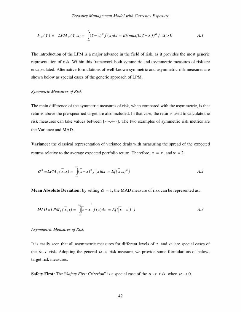
Bawa (1975) and Fishburn (1977) consolidated the existing research on risk measures up to that
time, and developed the α –t model, and introduced a general definition of “below target” risk in
the form of lower partial moments (LPM).
Let α be a parameter specifying the moment of the return distribution. In some cases α may be
taken as indicating different attitudes towards risk. Let τ be a predefined target level of the
investment return, and F(x) the cumulative probability distribution function of the investment with
return x. The LPM of order α for a given τ defines the α –t model and has the following form:
Treasury Management Model with Currency Exposure
42
F α (τ ) ≡ LPM α (τ ;x) = dxxfx )()( ατ
τ −∞−
= E(max[0, x−τ ])α , 0>α A.1
The introduction of the LPM is a major advance in the field of risk, as it provides the most generic
representation of risk. Within this framework both symmetric and asymmetric measures of risk are
encapsulated. Alternative formulations of well-known symmetric and asymmetric risk measures are
shown below as special cases of the generic approach of LPM.
Symmetric Measures of Risk
The main difference of the symmetric measures of risk, when compared with the asymmetric, is that
returns above the pre-specified target are also included. In that case, the returns used to calculate the
risk measures can take values between [- +∞∞, ]. The two examples of symmetric risk metrics are
the Variance and MAD.
Variance: the classical representation of variance deals with measuring the spread of the expected
returns relative to the average expected portfolio return. Therefore, τ = x , andα = 2.
2σ ≡ LPM 2 ( x ,x) = dxxfxx )()( 2−+∞
∞−
= E( x ,x) 2 A.2
Mean Absolute Deviation: by setting α = 1, the MAD measure of risk can be represented as:
MAD ≡ LPM 1 ( x ,x) = dxxfxx )(1
+∞
∞−
− = E( x - x ) 1 A.3
Asymmetric Measures of Risk
It is easily seen that all asymmetric measures for different levels of τ and α are special cases of
the α -τ risk. Adopting the general α -τ risk measure, we provide some formulations of below-
target risk measures.
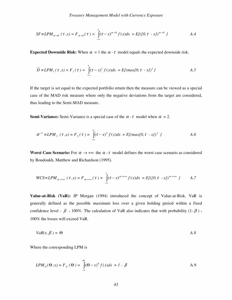
Safety First: The “Safety First Criterion” is a special case of the α -τ risk when .0→α
Treasury Management Model with Currency Exposure
43
SF ≡ LPM 0→α (τ ,x) = F 0→α (τ ) = dxxfx )()( 0→
∞−
−α
τ
τ = E([0,τ - x]) 0→α A.4
Expected Downside Risk: When α = 1 the α -τ model equals the expected downside risk.
D ≡ LPM 1 (τ ,x) = F 1 (τ ) = dxxfx )()( 1−∞−
τ
τ = E(max[0,τ - x])1 A.5
If the target is set equal to the expected portfolio return then the measure can be viewed as a special
case of the MAD risk measure where only the negative deviations from the target are considered,
thus leading to the Semi-MAD measure.
Semi-Variance: Semi-Variance is a special case of the α -τ model when α = 2.
2−σ ≡ LPM 2 (τ ,x) = F 2 (τ ) = dxxfx )()( 2−∞−
τ
τ = E(max[0,τ - x]) 2 A.6
Worst Case Scenario: For α +∞→ the α -τ model defines the worst case scenario as considered
by Boudoukh, Matthew and Richardson (1995).
WCS ≡ LPM +∞→α (τ ,x) = F +∞→α (τ ) = dxxfx )()( +∞→
∞−
−α
τ
τ = E([0,τ - x]) +∞→α A.7
Value-at-Risk (VaR): JP Morgan (1994) introduced the concept of Value-at-Risk. VaR is
generally defined as the possible maximum loss over a given holding period within a fixed
confidence level - β x 100%. The calculation of VaR also indicates that with probability (1- β ) x
100% the losses will exceed VaR.
VaR(x, β ) = Θ A.8
Where the corresponding LPM is
LPM 0 ( Θ ;x) = F 0 ( Θ ) = dxxfx )()( 0−ΘΘ
∞−
= 1 - β A.9
Treasury Management Model with Currency Exposure
44
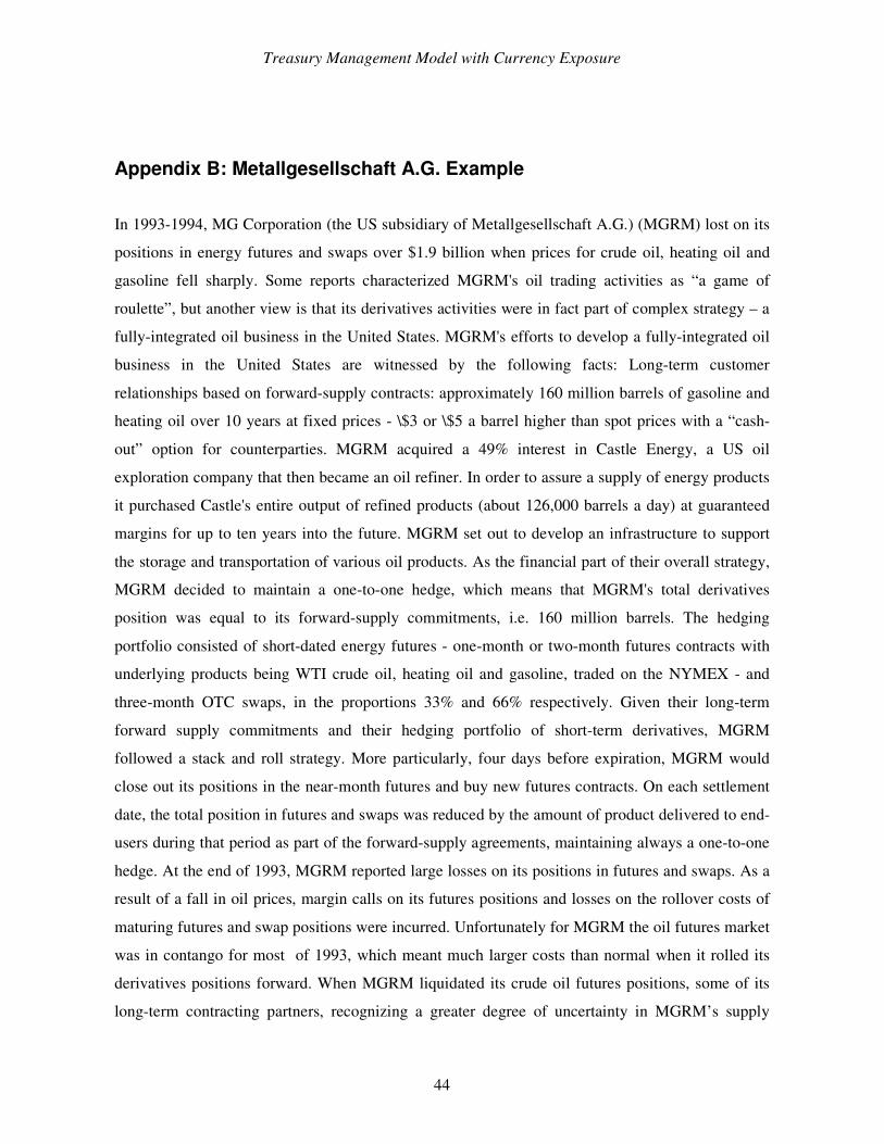
Appendix B: Metallgesellschaft A.G. Example
In 1993-1994, MG Corporation (the US subsidiary of Metallgesellschaft A.G.) (MGRM) lost on its
positions in energy futures and swaps over $1.9 billion when prices for crude oil, heating oil and
gasoline fell sharply. Some reports characterized MGRM's oil trading activities as “a game of
roulette”, but another view is that its derivatives activities were in fact part of complex strategy – a
fully-integrated oil business in the United States. MGRM's efforts to develop a fully-integrated oil
business in the United States are witnessed by the following facts: Long-term customer
relationships based on forward-supply contracts: approximately 160 million barrels of gasoline and
heating oil over 10 years at fixed prices - \$3 or \$5 a barrel higher than spot prices with a “cash-
out” option for counterparties. MGRM acquired a 49% interest in Castle Energy, a US oil
exploration company that then became an oil refiner. In order to assure a supply of energy products
it purchased Castle's entire output of refined products (about 126,000 barrels a day) at guaranteed
margins for up to ten years into the future. MGRM set out to develop an infrastructure to support
the storage and transportation of various oil products. As the financial part of their overall strategy,
MGRM decided to maintain a one-to-one hedge, which means that MGRM's total derivatives
position was equal to its forward-supply commitments, i.e. 160 million barrels. The hedging
portfolio consisted of short-dated energy futures - one-month or two-month futures contracts with
underlying products being WTI crude oil, heating oil and gasoline, traded on the NYMEX - and
three-month OTC swaps, in the proportions 33% and 66% respectively. Given their long-term
forward supply commitments and their hedging portfolio of short-term derivatives, MGRM
followed a stack and roll strategy. More particularly, four days before expiration, MGRM would
close out its positions in the near-month futures and buy new futures contracts. On each settlement
date, the total position in futures and swaps was reduced by the amount of product delivered to end-
users during that period as part of the forward-supply agreements, maintaining always a one-to-one
hedge. At the end of 1993, MGRM reported large losses on its positions in futures and swaps. As a
result of a fall in oil prices, margin calls on its futures positions and losses on the rollover costs of
maturing futures and swap positions were incurred. Unfortunately for MGRM the oil futures market
was in contango for most of 1993, which meant much larger costs than normal when it rolled its
derivatives positions forward. When MGRM liquidated its crude oil futures positions, some of its
long-term contracting partners, recognizing a greater degree of uncertainty in MGRM’s supply
Treasury Management Model with Currency Exposure
45
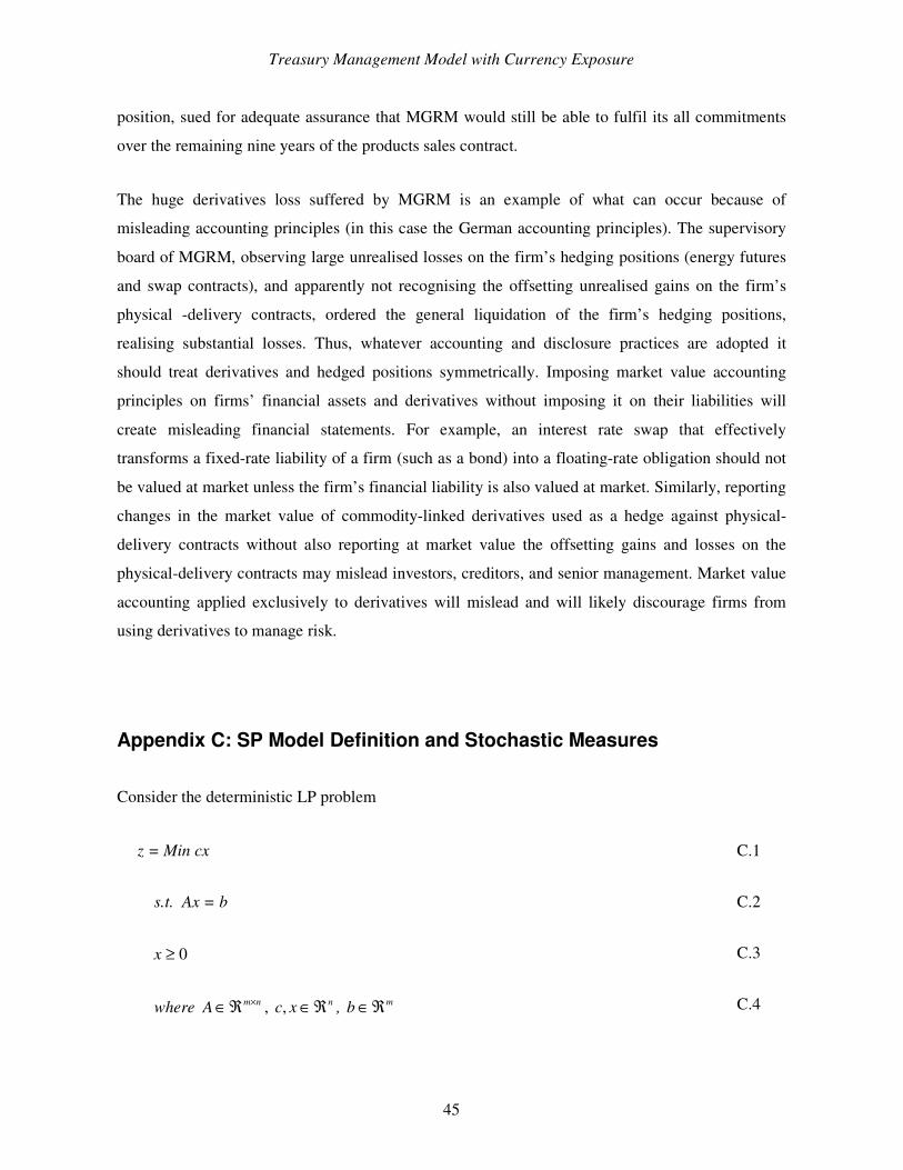
position, sued for adequate assurance that MGRM would still be able to fulfil its all commitments
over the remaining nine years of the products sales contract.
The huge derivatives loss suffered by MGRM is an example of what can occur because of
misleading accounting principles (in this case the German accounting principles). The supervisory
board of MGRM, observing large unrealised losses on the firm’s hedging positions (energy futures
and swap contracts), and apparently not recognising the offsetting unrealised gains on the firm’s
physical -delivery contracts, ordered the general liquidation of the firm’s hedging positions,
realising substantial losses. Thus, whatever accounting and disclosure practices are adopted it
should treat derivatives and hedged positions symmetrically. Imposing market value accounting
principles on firms’ financial assets and derivatives without imposing it on their liabilities will
create misleading financial statements. For example, an interest rate swap that effectively
transforms a fixed-rate liability of a firm (such as a bond) into a floating-rate obligation should not
be valued at market unless the firm’s financial liability is also valued at market. Similarly, reporting
changes in the market value of commodity-linked derivatives used as a hedge against physical-
delivery contracts without also reporting at market value the offsetting gains and losses on the
physical-delivery contracts may mislead investors, creditors, and senior management. Market value
accounting applied exclusively to derivatives will mislead and will likely discourage firms from
using derivatives to manage risk.
Appendix C: SP Model Definition and Stochastic Measures
Consider the deterministic LP problem
z = Min cx C.1
s.t. Ax = b C.2
x ≥ 0 C.3
where nmA ×ℜ∈ , nxc ℜ∈, , mb ℜ∈ C.4
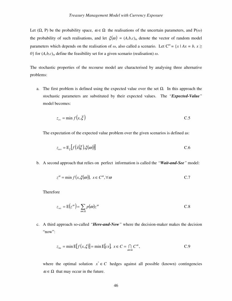
Treasury Management Model with Currency Exposure
46
Let (, P) be the probability space, Ω∈ω the realisations of the uncertain parameters, and P()
the probability of such realisations, and let ( )ωξ = (A,b,c) denote the vector of random model
parameters which depends on the realisation of , also called a scenario. Let C = x | Ax = b, x
0 for (A,b,c) define the feasibility set for a given scenario (realisation) .
The stochastic properties of the recourse model are characterised by analysing three alternative
problems:
a. The first problem is defined using the expected value over the set . In this approach the
stochastic parameters are substituted by their expected values. The “Expected-Value”
model becomes:
( )ξ,min xfzev = C.5
The expectation of the expected value problem over the given scenarios is defined as:
( ) ( )( )[ ]ωξξξ ,xfzeev Ε= C.6
b. A second approach that relies on perfect information is called the “Wait-and-See” model:
( )( ) ωωξ ωω ∀∈= , ,,min Cxxfz C.7
Therefore
( ) ( ) Ω∈
=Ε=ω
ωω ω zpzzws C.8
c. A third approach so-called “Here-and-Now” where the decision-maker makes the decision
“now”:
( )[ ] [ ] ω
ωξ CCxcxxfzhn
Ω∈=∈Ε=Ε= ,min,min , C.9
where the optimal solution Cx ∈* hedges against all possible (known) contingencies
Ω∈ω that may occur in the future.
Treasury Management Model with Currency Exposure
47
To assume the expected value scenario will occur and accept the solution of the expected value
problem, is not always the right decision, since the expected value might be far from the scenario
that actually takes place. The Wait-and-See problem cannot be implemented in reality, as the
decision-maker must wait to take the decision only when the uncertainty is resolved. This is not
realistic, since the decision-maker needs to decide before hand. Thereafter, to consider at a time all
the possible (known) scenarios, so-called the Here-and-Now approach, is the most appropriate,
since it hedges against all the uncertain future outcomes. The solution that this model provides is
not optimum for any one outcome, but is the best for many outcomes considered altogether.
To verify whether the stochastic approach is better than any other, some SP analysis must be carried
out. The analysis of stochastic programming models requires that we
(i) investigate the underlying expected value (EV) problem, and
(ii) compute stochastic information, such as the Expected Value of Perfect Information
(EVPI), and the Value of the Stochastic Solution (VSS) defined below:
(a) Expected Value of Perfect Information (EVPI):
EVPI measures the maximum amount a decision-maker would be ready to pay in return for
complete (and accurate) information about the future.
Let zhn = ( )ξξ ,min xfx
Ε , and zws = ( )[ ]ξξ ,min xfx
Ε then:
EVPI = zhn – zws C.10
(b) Value of the Stochastic Solution (VSS):
Let EV = ( )ξ,min xzx
, where ( )ξξ Ε= , and ( )ξx an optimal solution to the EV problem. Let
EEV = ( )( )[ ]ξξξ ,xfΕ C.11
Treasury Management Model with Currency Exposure
48
Then, VSS measures the cost of ignoring uncertainty in choosing a decision and is defined
as:
VSS = zeev – zhn. C.12
It can be shown that the three objective function values ZEEV, ZHN, ZWS are connected by the
following ordered relationship:
≤≤ C.13
The inequality:
≤ C.14
can be argued in the following way: any feasible solution of the average value approximation is
already considered in the Here and Now model, therefore the optimal Here and Now objective must
be better.
Bounds on EVPI and VSS
Some useful bounds on the EVPI and VSS are presented below:
EVEEVEVHN ZZZZEVPI −≤−≤≤0 C.15
−≤≤0 C.16
These can help in estimating the relative benefit of implementing the computationally costly
Stochastic Programming solution, as opposed to approximate solutions obtained by processing the
Expected Value LP problem.