Traversals of Object Structures: Specification and Efficient

Implementation∗

Karl Lieberherr

lieber@ccs.neu.edu

College of Computer Science

Northeastern University

Boston, MA 02115

USA

Boaz Patt-Shamir

boaz@eng.tau.ac.il

Dept. of Electrical Engineering

Tel-Aviv University

Tel-Aviv 69978

ISRAEL

Doug Orleans

dougo@ccs.neu.edu

College of Computer Science

Northeastern University

Boston, MA 02115

USA

March 7, 2004

Abstract

Separation of concerns and loose coupling of concerns are important issues in software engin-

nering. In this paper we show how to separate traversal-related concerns from other concerns, how

to loosely couple traversal-related concerns to the structural concern and how to efficiently imple-

ment traversal-related concerns. The stress is on the detailed description of our algorithms and the

traversal specifications they operate on.

Traversal of object structures is a ubiquitous routine in most types of information processing.

Ad-hoc implementations of traversals lead to scattered and tangled code and in this paper we present

a new approach, called traversal strategies, to succinctly modularize traversals. In our approach

traversals are defined using a high-level directed graph description, which is compiled into a dynamic

road map to assist run-time traversals. The complexity of the compilation algorithm is polynomial

in the size of the traversal strategy graph and the class graph of the given application. Prototypes of

the system have been developed and are being successfully used to implement traversals for Java and

AspectJ [KHH+01] and for generating adapters for software components. Our previous approach,

called traversal specifications [Lie92, PXL95], was less general, less succinct, and its compilation

algorithm was of exponential complexity in some cases. In an additional result we show that this

bad behavior is inherent to the static traversal code generated by previous implementations, where

traversals are carried out by invoking methods without parameters.

∗Research supported by Defense Advanced Projects Agency (DARPA) and Rome Laboratory under agreements

F30602-96-0239 and F33615-00-C-1694 and NSF Grant CCR 0098643.

1 Introduction

1.1 The Idea of Adaptive Traversals

The run-time state of application programs, particularly of object-oriented programs, can be repre-

sented as a directed graph, where objects are represented as nodes and field references are represented

as edges. To a large extent, program execution can be viewed as traversing that graph. Examples of

traversals are that sub-objects with certain properties are sought; or it may be desired to compute

a function of certain sub-objects of a given object. In standard programming techniques, expressing

traversals involves a strong commitment to the whole class structure traversed (since each hop in the

traversal is explicitly coded as in “a.b”), even if the task to be performed by the traversal depends

only on the start and the target objects.

We call a concern that deals with traversing objects for implementing some behavior of those

objects a traversal-related concern. A typical program operating on large sets of objects contains many

traversal-related concerns. Those traversal concerns already exist at the design level and become more

refined as we move from the design object structure to the implementation object structure. The

ad-hoc way for an experienced programmer to implement a traversal concern is to write methods for

each of the classes whose objects are traversed. Unfortunately, this leads to a scattered and tangled

implementation because the methods that implement the concern are spread across multiple classes

and tangled with methods from other concerns.

In this paper we propose a new paradigm, called traversal strategies, or strategies for short, which

helps us to not only cleanly modularize traversal-related concerns but also to minimally bind them

to the structural concern; i.e., strategies allow the programmer to specify traversals in a localized

manner with minimal binding to the class structure. Informally, the idea is to specify the high-level

topology of the traversal, in which only the key “milestones” are explicitly mentioned; given a concrete

class structure, executable traversal code is compiled, with all details filled in. Since the traversal is

minimally bound to the class structure, changes to the class structure will often require minimal or

no changes to the traversal strategy.

Strategies are a generalized form of traversal specifications, which were introduced in a simple form

in [Lie92] and formally treated in a more general form in [PXL95]. Succinct specifications of traversals

are an integral part of Adaptive Programming (AP) [Lie96].

1.2 Example

To give a more concrete flavor for the usefulness of strategies, let us demonstrate with the following

simple example.

Consider a program simulating bus route management. For expressing class graphs, we use the class

dictionary graph graphical representation from the Demeter method [Lie96]. Alternative notations

would be the UML class diagram notation [BRJ99] or an XML schema notation [Con]. For expressing

behavior, we use standard Java and the DJ library [OL01, LOO01, Lieb], a Java implementation of

the algorithms in this paper (see Section 7.2.2 for more details about DJ and our other software).

1

NonEmptyPersonList

PersonList

BusRoute

EmptyBusList

NonEmptyBusList

Bus BusStop

EmptyPersonList

Person

BusStopListBusList

buses busStops

first first

first

rest rest

rest

waiting

NonEmptyBusStopList

passengers

EmptyBusStopList

Figure 1: Bus simulation class graph. Squares and hexagons denote classes (concrete and abstract,

respectively), regular arrows denote field reference and are labeled by the field name, and heavy arrows

(labeled with ) denote the subclass relation (for the shading, see text).

Consider the class graph depicted in Figure 1, which defines a data structure describing a bus route.

A bus route object consists of two lists: a list of bus objects, each containing a list of passengers; and a

list of bus stop objects, each containing a list of people waiting. Suppose that as a part of a simulation,

we would like to determine the set of person objects corresponding to people waiting at any bus stop

on a given bus route. The group of collaborating classes which is needed for this task is shaded in

Figure 1. To carry out the simulation, an object-oriented program would contain a method for each of

these shaded classes. These methods that are scattered across several classes would traverse bus route

objects. However, using the technique of strategies, one can solve the problem in a much more elegant

way, by modularizing the code and keeping it in one place, rather than scattered through several

classes and tangled with other methods. We define a strategy graph with nodes BusRoute, BusStop

and Person that are connected by an edge from BusRoute to BusStop and an edge from BusStop to

Person. In our textual syntax, the strategy can be expressed as:

from BusRoute via BusStop to Person

The benefit of strategies is apparent when considering the following scenario: Suppose that the bus

route class has been modified so that the bus stops are grouped by villages. The revised class graph is

depicted in Figure 2. To implement the same requirement of finding all people waiting for a bus, an

object-oriented program must now contain one method for each of the classes shaded in Figure 2, and

thus the previous object-oriented implementation becomes invalid. The traversal strategy, however,

is up-to-date and does not require any rewriting. In fairness, the revision to the class graph must

preserve the class names referred to in the traversal strategy and the meaning of the traversal strategy

2

NonEmptyPersonList

PersonList

BusRoute

EmptyPersonList

Person

buses

first

BusStop

BusStopList

firstrest

rest

waiting

EmptyBusList

NonEmptyBusList

Bus

BusList

first restfirstrest

VillageList

NonEmptyVillageList

Village

villages

busStops

NonEmptyBusStopList

EmptyVillageList

passengers

EmptyBusStopList

Figure 2: Evolved bus simulation class graph.

must be correct for the new class graph. When a class graph is changed, it is important to check the

correctness of all traversal strategies that depend on that class graph. Sometimes it is necessary to

refine the strategies to make them correct in the new class graph, but this is easier than updating all

traversal methods manually [Lie96].

The actual work on the objects is done by methods on a visitor object: these are methods that can

be associated with classes or edges in the class graph, specifying what to do when the traversal arrives

at an object of a particular type or dereferences a particular field. Visitor objects are named after the

Visitor design pattern [GHJV95] but are much simpler than visitor objects described by the Visitor

design pattern, since none of the scaffolding is needed—by scaffolding we mean writing an abstract

visitor class that duplicates much information from the class graph.

Strategies effectively filter out the noise in the class graph which is irrelevant to the implemen-

tation of the current task. For the class graph in Figure 2, the above strategy, which mentions only

three classes, replaces methods for ten classes: BusRoute, VillageList, NonEmptyVillageList, Village,

BusStopList, NonEmptyBusStopList, BusStop, PersonList, NonEmptyPersonList, Person.

To show how to program with strategies, we complete the Java program (using the DJ library) of

finding all people waiting at any bus stop on a particular bus route:

// in class BusRoute:

static ClassGraph cg = new ClassGraph();

static Strategy waiting = new Strategy("from BusRoute via BusStop to Person");

void printWaitingPersons()

cg.traverse(this, waiting, new PrintVisitor());

3

The program above defines a method called printWaitingPersons for the class BusRoute. This method

will execute the traversal specified by the strategy and print the object of class BusRoute using the

visitor class PrintVisitor. Note that the definition of printWaitingPersons works without any change for

both class graphs, which is the reason for calling it an adaptive method [LOO01].

Notice that the adaptive method is expressed in plain Java using the DJ library of which we use the

classes ClassGraph and Visitor, the superclass of all visitor classes (such as PrintVisitor). A ClassGraph-

object is a graph whose nodes are classes and whose edges are is-a and has-a relationships between

classes. Class ClassGraph provides methods to create and maintain a class graph. The simplest way

to create a ClassGraph-object is to call the constructor ClassGraph() without arguments which will

create the class graph using Java reflection by taking all classes in the default package. A traversal

strategy may be applied to both a ClassGraph-object and a Java object. From the point of view of a

ClassGraph-object, a traversal strategy is a subgraph of the transitive closure of the ClassGraph-object.

When it is applied to a class graph it selects a subset of the paths in the class graph. If applied to a

Java object, a traversal strategy defines a subgraph of the object graph representing the Java object.

In this implementation of adaptive programming with DJ the class graph and the traversals are

computed dynamically. In other implementations of adaptive programming (see Section 7.2), the

traversals are computed statically.

To show the details of visitors, we write a Java method that counts (instead of prints) all people

waiting at any bus stop on a particular bus route. Because the traversals for printWaitingPersons and

countWaitingPersons are identical, we reuse the same waiting traversal strategy. We also reuse the class

graph cg:

// in class BusRoute:

int countWaitingPersons()

Integer result = (Integer) cg.traverse(this, waiting, new CountVisitor());

return result.intValue();

class CountVisitor extends Visitor

int c;

public void start() c = 0;

public void before(Person p) c++;

public Object getReturnValue() return new Integer(c);

Class Visitor has a simple interface: with the start method we say what needs to be done before the

traversal starts. With the getReturnValue method we express what needs to be returned when the

traversal completes. With a before method we express what needs to be done before we visit an object

of a specific class, specified by the method’s argument type. There are also after and around methods;

the complete API is documented in [Lieb]. The before, after, and around methods that are defined in

a visitor class are invoked using the Java Reflection API.

4

1.3 New Contributions

The contributions of this paper are three-fold: an extension to the traversal specification language,

a polynomial-time compilation algorithm for the extended language that is simpler than our earlier

algorithm, and a lower bound result which explains the shortcomings of the previous algorithms. More

specifically, we allow the underlying specification of a traversal to have any topology, generalizing the

series-parallel and tree topologies considered previously, and we allow the use of a name map between

nodes in the strategy graph and those in the class graph. This name map supports the option for

different nodes in the strategy graph to be mapped to the same node in the class graph. Section 9

provides a more detailed comparison of traversal strategies and traversal specifications.

The generalization of our previous algorithm to a larger class of graphs was not our primary goal

for coming up with a better algorithm. It happened as a side-effect: as we made the algorithm more

efficient and usable for a larger class of series-parallel graph/class graph combinations, the resulting

algorithm also naturally worked for any kind of graph.

Our new polynomial-time algorithm presented in Section 5 has the beneficial property that it is

simpler and easier to understand. Our earlier algorithm required an unintuitive check for the short-

cut and zig-zag conditions. Those two conditions had to be checked to make sure that the traver-

sal is correct. The short-cut and zig-zag conditions also prohibited many series-parallel graph/class

graph combinations. We notice that this paper is related to two applications of Polya’s inventors

paradox[Pol49]:

1. Although we solve a more general algorithmic problem at the programming tool level, the algo-

rithm becomes simpler.

2. The algorithm supports better adaptive programming which is about solving problems for more

general data structures than the one originally given, leading to simpler programs ([Lie96],

Section 4.1.1).

The compilation algorithm generates code whose running time may be slightly worse than the

running time of the code generated by previous compilation algorithms (when they apply), since the

previous algorithm generated traversal methods which did not pass arguments at all. However, this

minor penalty in running time is unavoidable if we want the size of the traversal code to be reasonably

bounded: we prove in Section 6 that if no arguments are passed by the traversal methods, then there

are cases where the number of distinct traversal methods must be exponential in the size of the strategy

specification.

1.4 Algorithm Overview

For those readers who don’t need to understand all the details behind the algorithms we give a brief

overview. Given a strategy S and a class graph G, we need to provide an algorithm that decides

which objects to visit from a node o in an object graph, i.e., we need to compute first(o), the set of

edges that we need to traverse from node o. The function first(o) is computed based on answers to

reachability questions in the class graph; it contains all edges that could lead (according to the rules

5

of the class graph) to target objects. The “could” represents our lack of knowledge about the rest

of the object graph [LW01]. More precisely, first(o) contains all edges ol→ o′ such that there exists

an object graph rooted at o′ that contains a target object and that satisfies a fixed set of constraints

(expressed by S and G).

Our goal is to make the traversal efficient; therefore we don’t want to look ahead in the object

graph to decide whether going through an edge in first(o) will eventually lead us to a target object.

We only look ahead in the class graph because it gives us meta-information about the shape of objects.

So first(o) will contain all those edges after which, according to the class graph information, there is

still a possibility of reaching a target object. To quickly answer the reachability questions we compute

a new graph, called a traversal graph, which is basically the product of the two graphs S and G. The

traversal graph stores the answers to the reachability questions that we will ask during the object

traversal.

The Traversal Graph Algorithm (TGA) is based on the following idea of a reduction: For traversal

strategies of the form “from A to B”, the paths defined in the class graph can be represented by a

subgraph of the class graph: Compute all edges reachable from A (called forward edges) and from

which B can be reached (called backward edges). This computation is called from-to computation.

Edges in the intersection of the forward and backward edges form the graph which represents the

traversal. Any strategy can be reduced to a from-to computation on a graph that is much larger

than the original class graph. This larger graph, called the traversal graph, will contain as many

copies of the class graph as the traversal strategy graph has edges. The size of the traversal graph

will be reduced by a from-to computation. In other words, the from-to computation (which can be

implemented, e.g., with a forward and a backward depth-first search) is fundamental to computing

the traversal graph. The size of the traversal graph is a small polynomial in the size of the class graph

and the strategy graph.

The traversal graph is non-deterministic in nature: from a node there might be two outgoing edges

with the same label (leading to different nodes—there are no parallel edges). This non-determinism

needs to be handled carefully in order to avoid an exponential blow-up in algorithm performance. The

Traversal Methods Algorithm (TMA) traverses an object graph, guided by a traversal graph. To deal

with the non-determinism, we allow multiple tokens simultaneously to be put on the traversal graph to

keep track of the legal traversal possibilities. As the traversal progresses the number of tokens on the

traversal graph fluctuates. Fortunately, the number of simultaneous tokens is bounded by the number

of edges in the strategy graph.

As suggested by [PPL97, Sma], these two algorithms are about computing intersections of sets

of paths. TGA is a variation on an algorithm to compute the cross product of two automata, while

TMA is inspired by the NFA simulation technique described in [ASU86]. The complications are in

the constraint maps, the name maps and the more complex structure of the graphs: class graphs have

two kinds of nodes and two kinds of edges.

6

1.5 Paper Organization

The remainder of this paper is organized as follows. In Section 2 we introduce the basic concepts,

terminology and notation we use throughout the paper. In Section 3 we give a definition for the

concept of traversals, based on [PPL97]. In Section 4 we define the new concept of strategies. In

Section 5 we specify and analyze the algorithm which translates strategies into traversal code. In

Section 6 we prove a lower bound for traversal methods that do not pass arguments. In Section 7 we

comment about some practical aspects of the implementation of the strategies approach. In Section

8 we survey related work. In Section 9 we compare strategies with the earlier approach of traversal

specifications. In Section 10 we describe some applications of strategies. In Section 11 we describe our

experiences using strategies and present some empirical evidence of how they are used. We give a few

concluding thoughts in Section 12.

2 Preliminaries

In this section we formally define the basic concepts, terminology and notation we use throughout this

paper. All notions in this section are standard, with the exception of Subsection 2.3.

2.1 Graphs and paths

A directed graph is a pair (V, E) where V is a set of nodes, and E ⊆ V × V is a set of edges. A

directed labeled graph is a triple G = (V, E, L) where V is a set of nodes, L is a set of labels, and

E ⊆ V ×L× V is a set of edges. If e = (u, l, v) ∈ E, then u is the source of e, l is the label of e, and v

is the target of e. We denote an edge (u, l, v) by ul→ v.

Given a directed labeled graph G = (V, E, L), a node-path is a sequence p = 〈v0v1 . . . vn〉, where

vi ∈ V for 0 ≤ i ≤ n, and vi−1li→ vi ∈ E for some li ∈ L for all 0 < i ≤ n. Similarly, a path is

a sequence 〈v0l1v1l2 . . . lnvn〉 where 〈v0 . . . vn〉 is a node-path, and vi−1li→ vi ∈ E for all 0 < i ≤ n.

Unlabeled graphs have only node-paths. Paths of the form 〈v0〉 are called trivial. The first node of

a path (or a node-path) p is called the source of p, and the last node in p is called the target of p,

denoted Source(p) and Target(p), respectively. The elements other than the source and the target of

a path (nodes for a node-path, nodes and edges for a path) are the interior of the path. For a graph

G, nodes u, v, and sets of nodes U, V , we define PG(u, v) to be the set of all paths in G with source u

and target v and PG(U, V ) to be the set of all paths in G with source in U and with target in V .

If p1 = 〈v0 . . . livi〉 and p2 = 〈vili+1 . . . vn〉 are paths with the target of p1 identical to the source

of p2, we define the concatenation p1 · p2 = 〈v0 . . . vi−1livili+1vi+1 . . . vn〉. Notice that p1 · p2 contains

only one copy of the meeting point vi. Concatenation of node paths is defined similarly. Let P1 and

P2 be sets of paths such that for some node v, Target(p1) = v for all p1 ∈ P1, and Source(p2) = v for

all p2 ∈ P2. Then we define

P1 · P2 = p1 · p2 | p1 ∈ P1 and p2 ∈ P2 .

7

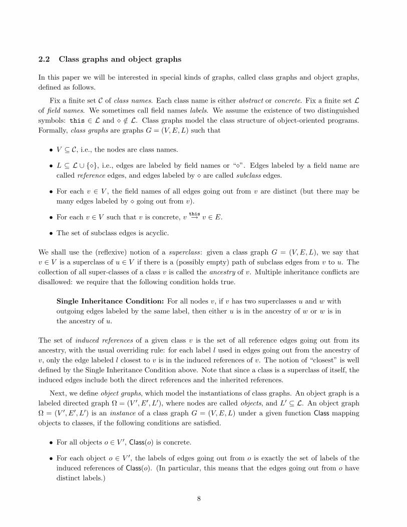
2.2 Class graphs and object graphs

In this paper we will be interested in special kinds of graphs, called class graphs and object graphs,

defined as follows.

Fix a finite set C of class names. Each class name is either abstract or concrete. Fix a finite set L

of field names. We sometimes call field names labels. We assume the existence of two distinguished

symbols: this ∈ L and /∈ L. Class graphs model the class structure of object-oriented programs.

Formally, class graphs are graphs G = (V, E, L) such that

• V ⊆ C, i.e., the nodes are class names.

• L ⊆ L ∪ , i.e., edges are labeled by field names or “”. Edges labeled by a field name are

called reference edges, and edges labeled by are called subclass edges.

• For each v ∈ V , the field names of all edges going out from v are distinct (but there may be

many edges labeled by going out from v).

• For each v ∈ V such that v is concrete, vthis→ v ∈ E.

• The set of subclass edges is acyclic.

We shall use the (reflexive) notion of a superclass: given a class graph G = (V, E, L), we say that

v ∈ V is a superclass of u ∈ V if there is a (possibly empty) path of subclass edges from v to u. The

collection of all super-classes of a class v is called the ancestry of v. Multiple inheritance conflicts are

disallowed: we require that the following condition holds true.

Single Inheritance Condition: For all nodes v, if v has two superclasses u and w with

outgoing edges labeled by the same label, then either u is in the ancestry of w or w is in

the ancestry of u.

The set of induced references of a given class v is the set of all reference edges going out from its

ancestry, with the usual overriding rule: for each label l used in edges going out from the ancestry of

v, only the edge labeled l closest to v is in the induced references of v. The notion of “closest” is well

defined by the Single Inheritance Condition above. Note that since a class is a superclass of itself, the

induced edges include both the direct references and the inherited references.

Next, we define object graphs, which model the instantiations of class graphs. An object graph is a

labeled directed graph Ω = (V ′, E′, L′), where nodes are called objects, and L′ ⊆ L. An object graph

Ω = (V ′, E′, L′) is an instance of a class graph G = (V, E, L) under a given function Class mapping

objects to classes, if the following conditions are satisfied.

• For all objects o ∈ V ′, Class(o) is concrete.

• For each object o ∈ V ′, the labels of edges going out from o is exactly the set of labels of the

induced references of Class(o). (In particular, this means that the edges going out from o have

distinct labels.)

8

• For each edge ol→ o′ ∈ E′, Class(o) has an induced reference edge v

l→ u such that v is a

superclass of Class(o) and u is a superclass of Class(o′).

For the greater part of this paper, we shall assume that object graphs are acyclic. We discuss an

extension to cyclic object graphs in Section 5.4.

2.3 Non-standard notions

In this paper, we assume that class graphs are simple, formally defined as follows.

Definition 2.1 A class graph G = (V, E, L) is simple if

1. for all edges ul→ v ∈ E, we have that l = if and only if u is abstract, and

2. for all edges u→ v ∈ E, we have that v is concrete.

The first requirement says that all edges going out from abstract classes are subclass edges and all

edges going out from concrete classes are reference edges. This property is called flatness. Flatness

helps us map paths in a class graph G to paths in an object graph which is an instance of G. The

second requirement says that all subclass edges are coming into concrete classes; this helps us find all

subclasses of a given class quickly. Note that no generality is lost by the assumption that class graphs

are simple, as the following proposition asserts.

Proposition 2.1 Let G = (V, E, L) be an arbitrary class graph. Then there exists a simple class

graph Simplify(G) = (V ′, E′, L) such that an object graph Ω is an instance of G if and only if Ω is an

instance of Simplify(G). Moreover, |V ′| = O(|V |) and |E′| = O(|E|2).

The Simplify transformation is outlined in Appendix A. Note that the output of our compilation

algorithm is a set of methods on an arbitrary class graph, i.e. it need not be simple. An existing class

structure does not need to be modified to be used with our algorithm; it is only the graph representation

of the class structure that may need to be pre-processed by the Simplify transformation.

Define a concrete path to be an alternating sequence of concrete class names and labels (excluding

). We shall map paths in class graphs to concrete paths by omitting abstract classes and subclass

edges. We refer to this mapping as the natural correspondence, and denote it by X(p), where p is a

path in a class graph G and X(p) is the corresponding concrete path. Similarly, we denote the concrete

path resulting from taking the sequence of class names and edge labels in an object graph path p′ by

Y (p′), and (overloading the term) we call this mapping also a natural correspondence. The motivation

for these definitions is that if p is a path in a class graph G, then there is some object graph Ω which

is an instance of G, and a path p′ in Ω, such that X(p) = Y (p′).

For a class graph path set P , define X(P )def= X(p) | p ∈ P.

9

3 Definition of traversals

We now arrive at the central topic of this paper: traversals of object graphs. Informally, a traversal is

a (possibly infinite) set of concrete paths; when used in conjunction with an object graph, it results

in a sequence of objects, called the traversal history. The traversal history is a depth-first traversal of

the object graph along object paths agreeing with the given concrete path set. To make the traversal

useful, each object has a special visit method attached to it; when an object is added to the traversal

history, this method is invoked. (A more comprehensive discussion of the Visitor design pattern and

visitor methods can be found in [GHJV95, SPL96, SPL98].)

But first, we define traversals formally. The definition here is adapted from the “simplified seman-

tics” from [PPL97]. We use a few technical notions. For a set of sequences R ⊆ Σ∗ for an alphabet Σ,

define

head(R) = x ∈ Σ | ∃α.(xα ∈ R)

tail(R, x) = α | xα ∈ R for some x ∈ Σ .

Intuitively, head(R) is the set of all first elements of R, and tail(R, x) is the set of all “tails” of sequences

of R that start with x (where a tail of a sequence is the whole sequence except its first element).

In the definition below, we assume that there exists a total order ≺ on the set of field names L

(this assumption may be weakened somewhat). We first give the formal definition, then explain it in

words.

Definition 3.1 (from [PPL97]) Fix a class graph G. If Ω is an acyclic object graph which is an

instance of G, o an object in Ω, R a set of concrete paths corresponding to paths of G, and H a

sequence of objects, then the judgment

Ω `s o : R H

means that when traversing the object graph Ω starting with o, and guided by the concrete path set R,

then H is the traversal history.1 This judgment holds when it is derivable using the following rules:

Ω `s o : R εif tail(R, Class(o)) = ∅, (1)

where ε denotes the empty history, and

Ω `s oi : tail(tail(R, Class(o)), li) Hi ∀i ∈ 1..n

Ω `s o : R o ·H1 · ... ·Hn

if head(tail(R, Class(o))) = li | i ∈ 1..n,

oli→ oi is in Ω, i ∈ 1..n, and

lj ≺ lk for 1 ≤ j < k ≤ n.(2)

In other words, a traversal of an object graph Ω starting with an object o guided by a path set R, is

done as follows. First, the first elements of the sequences of R are compared to Class(o): sequences

beginning with another element are immediately thrown out of consideration. If the remaining path

set is not empty, then o becomes the first element of the history; it is followed by the histories resulting

from starting a traversal from each descendent of o, guided by the remainder of the path set after

1The label s of the turnstile indicates “semantics.”

10

“peeling off” the first two elements (corresponding to o and the edge going out to the descendent).

Intuitively, this procedure is depth-first search on Ω with R used to determine how to prune the search.

Please note that concatenation of traversal histories does not use the same definition as concatenation

of paths; it is the usual concatenation of sequences.

Remarks. Note that the guarantee made by a traversal guided by a path set R is the following: A

path p in the object graph is followed so long as there is a path q ∈ R such that q has a prefix which

is equal to the current prefix of p (taking the Class(o) instead of o in p). In other words, the decision

whether the traversal takes a certain branch in the object graph depends only on the portion of the

graph visited so far and on the current branch, and not on the links further ahead. This means, for

example, that even if all paths in R end with the same class A, some of the traversal paths may end

with a node o with Class(o) 6= A just because the path to o is a prefix of a path in R. This relaxation

is necessary to enable efficient implementation of traversals by looking only ahead in the class graph

and not in the object graph as discussed earlier.

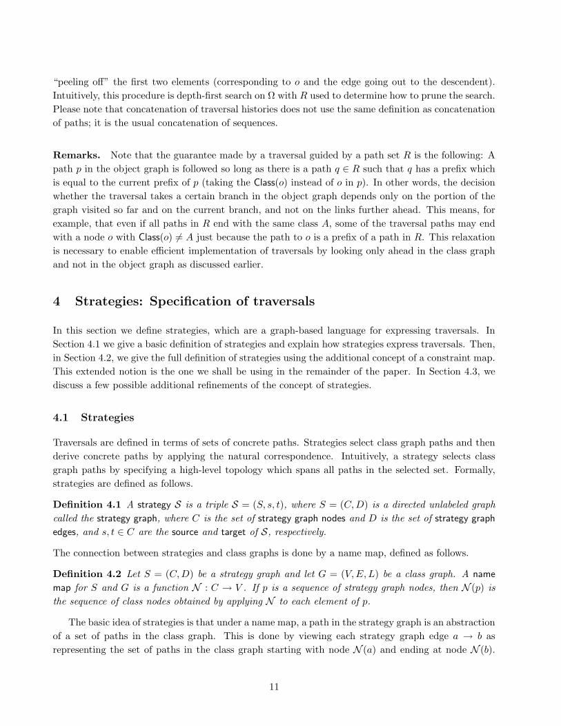
4 Strategies: Specification of traversals

In this section we define strategies, which are a graph-based language for expressing traversals. In

Section 4.1 we give a basic definition of strategies and explain how strategies express traversals. Then,

in Section 4.2, we give the full definition of strategies using the additional concept of a constraint map.

This extended notion is the one we shall be using in the remainder of the paper. In Section 4.3, we

discuss a few possible additional refinements of the concept of strategies.

4.1 Strategies

Traversals are defined in terms of sets of concrete paths. Strategies select class graph paths and then

derive concrete paths by applying the natural correspondence. Intuitively, a strategy selects class

graph paths by specifying a high-level topology which spans all paths in the selected set. Formally,

strategies are defined as follows.

Definition 4.1 A strategy S is a triple S = (S, s, t), where S = (C, D) is a directed unlabeled graph

called the strategy graph, where C is the set of strategy graph nodes and D is the set of strategy graph

edges, and s, t ∈ C are the source and target of S, respectively.

The connection between strategies and class graphs is done by a name map, defined as follows.

Definition 4.2 Let S = (C, D) be a strategy graph and let G = (V, E, L) be a class graph. A name

map for S and G is a function N : C → V . If p is a sequence of strategy graph nodes, then N (p) is

the sequence of class nodes obtained by applying N to each element of p.

The basic idea of strategies is that under a name map, a path in the strategy graph is an abstraction

of a set of paths in the class graph. This is done by viewing each strategy graph edge a → b as

representing the set of paths in the class graph starting with node N (a) and ending at node N (b).

11

This representation naturally extends to paths in the strategy graph: A path in the strategy graph

represents a set of paths in the class graph obtained by concatenating the sets of class graph paths

obtained from each strategy graph edge.

We now make this intuition formal using the concept of path expansion, defined as follows.

Definition 4.3 Given a nontrivial sequence p, a sequence is called an expansion of p if it can be

obtained by inserting one or more elements between the elements of p. The only expansion of a trivial

sequence is itself.

Note that if p′ is a path which is an expansion of another path p (possibly in another graph), then

Source(p) = Source(p′) and Target(p) = Target(p′).

We now formally define the basic way strategies express paths in object graphs. Recall that PG(s, t)

denotes that set of all paths in G starting at s and ending at t and X is the natural correspondence

mapping class graph paths to concrete paths.

Definition 4.4 Let S = (S, s, t) be a strategy, let G = (V, E, L) be a class graph, and let N be a name

map for S and G. Then

S[G,N ] =

X(p′) | p′ ∈ PG(N (s),N (t)) and ∃p ∈ PS(s, t) such that p′ is an expansion of N (p)

.

Note that S[G,N ] is a set of concrete paths: intuitively, first a set of class graph paths is selected,

and then the natural correspondence is applied to obtain concrete paths. These concrete paths can

be used (playing the role of “R”) in Definition 3.1.

4.2 Using a constraint map

Strategies impose positive constraints on paths, in the sense that they specify which nodes must be

traversed in which order. It turns out that it is quite useful to also have negative constraints: what

nodes and edges cannot be used between the specified milestones. We formalize this idea with the

concepts of element predicates and constraint maps.

Definition 4.5 Given a class graph G = (V, E, L), an element predicate EP for G is a predicate over

V ∪E. Given a strategy graph S, a function B mapping each edge of S to an element predicate for G

is called a constraint map for S and G.

(Of course, some predicate specification languages may be very hard to compute. For computational

complexity purposes, we assume that there exists a parameter, denoted τ , such that given an element

of G, determining whether it satisfies an element predicate can be computed in no more than τ time

units.)

The constraint map is used to specify, for each edge in the strategy graph, which elements of the

class graph may be used in the traversal corresponding to that edge. Formally, we have the following

definition.

Definition 4.6 Let S be a strategy graph, let G be a class graph, let N be a name map for S and G,

and let B be a constraint map for S and G. Given a strategy graph node path p = 〈a0a1 . . . an〉, we

12

say that a class graph path p′ is a satisfying expansion of p with respect to B under N if there exist

nontrivial paths p1, . . . , pn such that p′ = 〈N (a0)〉 · p1 · p2 · · · pn and:

1. For all 1 ≤ i ≤ n, Source(pi) = N (ai−1) and Target(pi) = N (ai).

2. For all 1 ≤ i ≤ n, the interior elements of pi satisfy the element predicate B(ai−1 → ai).

If n = 0, i.e., p is a trivial path 〈a0〉, then its only satisfying expansion is 〈N (a0)〉.

Note that there may be many ways to decompose a path in accordance with Condition 1 in the

definition above; a path p′ is a satisfying expansion of a path p if for one of these decompositions,

Condition 2 holds as well.2 Note also that the element constraints are never applied to the ends of the

sub-paths.

One consequence of our definition is that every edge in a strategy graph path corresponds to one

or more class graph edges in a satisfying expansion: if N (ai−1) = N (ai), the path pi may not be the

trivial path 〈N (ai)〉. A further consequence is that every class graph edge in a satisfying expansion

satisfies at least one element predicate in the constraint map.

Using the constraint map, we now define a more elaborate way in which a strategy expresses paths

in object graphs.

Definition 4.7 Let S = (S, s, t) be a strategy, let G = (V, E, L) be a class graph, let N be a name

map for S and G, and let B be a constraint map for S and G. Then S[G,N ,B] is the set of concrete

paths defined by

S[G,N ,B] =

X(p′) | p′ ∈ PG(N (s),N (t)) and

∃p ∈ PS(s, t) such that p′ is a satisfying expansion of p w.r.t. B

.

Note that S[G,N ] = S[G,N ,Btrue] for the constraint map Btrue which maps all strategy graph edges

to the trivial element predicate that is always true.

4.3 Remarks

Encapsulated strategies. The way strategies are presented above, a constraint map can be speci-

fied only when the class graph is given, as the element predicates are expressed in terms of class graph

nodes and edges. An important design consideration, however, is to encapsulate the constraint map

with the strategy and use the name map as the only interface to the class graph; we call this approach

“encapsulated strategies.” The advantage of encapsulated strategies is that they allow one to have a

clean interface between the strategy and the class graph, captured completely by the name map.

We only outline the details of the concept here, since it is not central to the algorithmic issues we

focus on in the remainder of this paper. The idea is that instead of letting the element predicates

2Other definitions are possible, for example to require that a subpath ends when its target node is reached. We have

found the non-deterministic definition above to be the most useful. Constraint maps can be used to reduce or eliminate

the non-determinism.

13

range over the (yet unspecified) class graph, they range over variables called symbolic names. Binding

to actual class graph elements is done only later, when the name map is introduced. Technically, we

have an additional level of indirection in the encapsulated strategy: instead of explicit references to

the class graph elements in the constraint map, the element predicates are predicates over symbolic

nodes and symbolic edges. These are denoted using a setM of strings, which are used as place-holders

for class names and labels (symbolic edges are constructed from a pair of symbolic node names and

a symbolic label). More formally, an encapsulated strategy is a tuple E = (S,M,B′), where S is a

strategy, M is a set of symbolic names, and B′ is a function mapping edges of the strategy graph to

predicates over the symbolic elements. To support encapsulated strategies, the name map is extended

to map also symbolic names to actual class names and label names in the class graph.

Wildcard notation in predicate specification. We left the issue of how to specify the predicates

open. One naive way of doing it is to enumerate all elements to be used, or alternatively to enumerate

all elements to be excluded (cf. “only-through” and “bypassing” clauses presented in Section 7.1).

More expressive power is given by allowing wildcard symbols to be used in the predicate specification.

For example, an element predicate may be false for all elements of the form ∗l→ ∗, which means

that no edges labeled l can be traversed. The unique feature of this notation is that it allows the

programmer to refer to elements whose identity is not necessarily known at predicate-specification

time. Even when using encapsulated strategies as above, the programmer can only refer to symbolic

names, which are later mapped to only a subset of the elements of the actual class graph, while the

wildcard notation is implicitly mapped to all elements in the class graph as appropriate.

There is a difference between the strategies used by the algorithm, on the one hand, and the data

structures available in our implementation (described in Section 7). In the former, strategy graph edges

are general, with a restriction only on the cost of verifying the governing condition per vertex and per

edge. In the latter, only a small set of predefined predicates are used (bypassing, only-through). The

reason for this difference is that we wanted the abstract model to be easy to express and it turned

out that a more general formulation is easier to express. The general model can easily handle the

particular edge predicates actually in use in the implementation. For the current applications the

expressive power of the model used by our implementation is sufficient. Indeed, when the class graph

is known, all strategies can be simulated by single edge strategies using bypassing clauses bypassing

sufficiently many nodes and edges in the class graph.

Cyclic graphs. Strategy graphs may be cyclic and so may class graphs and object graphs. However

for the purpose of dealing with traversals, it is sufficient to consider object trees. Non-object trees

need to be addressed by appropriate visitors. See Section 5.4 for more discussion.

5 Compilation algorithm

In this section we show how to implement traversal strategies efficiently by compiling them into

executable programs. Formally, the compilation problem is defined as follows.

14

Input: A strategy S = (S, s, t), a simple class graph G = (V, E, L), a name map N for S and G, and

a constraint map B for S and G.

Output: A set of methods such that for any object graph Ω, invoking the traversal method at an

object o in Ω yields a traversal history H satisfying the judgment Ω `s o : S[G,N ,B] H.

Recall that S[G,N ,B] is a path set which can guide traversals of object graphs directly. Our compi-

lation consists of two algorithms. For an overview of the algorithms see Section 1.4.

1. We first invoke an algorithm (called TGA below) which uses S, G, N , and B to construct a

graph which expresses the traversal S[G,N ,B] in a more convenient way; we call this graph the

traversal graph, and denote it by TG(S, G,N ,B).

2. We then generate traversal methods that employ another algorithm (called TMA below), which

uses TG(S, G,N ,B)—the result of TGA—at runtime.

The remainder of this section is organized as follows. In Section 5.1 we describe TGA. In Section 5.2 we

describe TMA. In Section 5.3 we analyze the computational complexity of the algorithms. We conclude

this section with numerous extensions and variants for the basic algorithm, listed in Section 5.4.

5.1 The traversal graph

In this section we explain how the traversal graph is computed, based on a strategy S = (S, s, t), a

simple class graph G = (V, E, L), a name map N for S and G, and a constraint map B for S and G.

The traversal graph, denoted TG(S, G,N ,B), is created by a series of transformations based on the

class graph, the strategy, the name map, and the constraint map. The basic idea is to replace each

strategy graph edge by a copy of the class graph appropriately pruned down to elements that satisfy

the edge’s element predicate.

The reader may follow a running example presented in Figure 3 (DJ code for the example is given

in Section 7).

Traversal Graph Algorithm (TGA): Let the strategy graph be S = (C, D), and let the strategy

graph edges be D = e1, e2, . . . , ek.

1. Create a graph G′ = (V ′, E′) by taking k copies of G, one for each strategy graph edge. Denote

the ith copy as Gi = (V i, Ei). We will use the correspondence between each strategy graph edge

ei and Gi. The nodes in V i and edges in Ei will be denoted with a superscript i, as in vi, ei etc.

Each class graph node v corresponds to k nodes in V ′, denoted v1, . . . , vk. We extend the Class

mapping to apply to the nodes of G′ by setting Class(vi)def= v, where vi ∈ V ′ and v ∈ V .

2. For each strategy graph edge ei = a → b: Let N (a) = u and N (b) = v. Remove from Gi the

15

targetsourceA Ee1 e2

e3 e4

2

D

Z

A B

ED Y Z

C

1c

b

d ez

y

3

A B

ED Y Z

C A B

ED Y Z

C

A B

ED Y Z

C B

ED Y Z

C

A B

ED Y Z

C A B

ED Y Z

C

A B

ED Y Z

C B

ED Y Z

C

s*

A

D Y

A B

D Y Z

C

A B

D Y Z

B

D Y Z

4

A B

ED Y

C A B

ED Y Z

C

A B

ED Y Z

C B

ED Y Z

C

5 6

Z

E*

E*

E*

Figure 3: An example of traversal graph computation. 1: the input class graph. Edge labels are

omitted from subsequent graphs. 2: The input strategy (the name map is indicated). In this example,

the constraint map is as follows: B(e1)(Bz→ Z) = false and B(e1)(x) = true for all x 6= B

z→ Z;

B(e2)(x) = true for all x; B(e3)(Ad→ D) = false and B(e3)(x) = true for all x 6= A

d→ D; and

B(e4)(x) = false if x = A or if x is an edge incident to A, and B(e4)(x) = true otherwise. 3: G′

after Steps 1 and 2. 4: G′ after Steps 3a and 3b. Intercopy edges are dashed. 5: G′ after Steps 3c, 3d,

and 4. 6: The final traversal graph, as returned in Step 6. The shaded A nodes are the start set Ts,

and the shaded node E∗ is the finish set Tf .

16

elements which do not satisfy B(ei). More precisely, set

V i ←

ui, vi

∪

wi | B(ei)(w) = true

, and

Ei ←

ui l→ vi | B(ei)(u

l→ v) = true

∪

ui l→ yi | B(ei)(u

l→ y) = B(ei)(y) = true

∪

wi l→ vi | B(ei)(w

l→ v) = B(ei)(w) = true

∪

wi l→ yi | B(ei)(w

l→ y) = B(ei)(w) = B(ei)(y) = true

.

3. (a) For each strategy graph node a ∈ C: Let I = ei1 , . . . , ein be the set of strategy graph

edges coming into a, and let O = eo1, . . . , eom be the set of strategy graph edges going

out from a. Let N (a) = v ∈ V . Add to G′ n · m edges vij → vol for j = 1, . . . , n and

l = 1, . . . , m. Call these edges intercopy edges.

(b) Add to G′ a node N (t)∗ and, for each edge ei coming into the target node t in S, an

intercopy edge N (t)i → N (t)∗.

(c) For each node vi in G′ with an outgoing intercopy edge: Add to G′ edges ui l→ vj for all ui

and vj such that ui l→ vi ∈ Ei and vi → vj is an intercopy edge.

(d) Remove all the intercopy edges added in Steps 3a and 3b.

4. Add to G′ a node s∗ and, for each edge ei going out from the source node s in S, an edge

s∗ → N (s)i. If s = t, add to G′ an edge s∗ → N (t)∗.

5. Mark all nodes and edges in G′ which are both reachable from s∗ and from which N (t)∗ is

reachable, and remove unmarked nodes and edges from G′. Call the resulting graph G′′ =

(V ′′, E′′).

6. Return the following objects:

• The set of all nodes v such that s∗ → v is an edge in G′′. This is the start set, denoted Ts.

• The graph obtained from G′′ after removing s∗ and all its incident edges. This is the

traversal graph, denoted TG(S, G,N ,B).

For the purpose of analysis, we also define the finish set of the traversal graph, denoted Tf , to be the

singleton set containing the node N (t)∗.

Correctness

We now prove that TGA is correct, in the sense that the set of paths in the traversal graph (from the

start set to the finish set) is exactly the set of paths defined by the strategy. This property is formally

stated in Lemma 5.2.

First, we show a basic property of paths in the traversal graph.

Lemma 5.1 If p is a path in the traversal graph, then under the extended Class mapping, p is a path

in the class graph.

17

Proof: Note that for any edge ui l→ vj in the traversal graph, we have that the corresponding edge

ul→ v is in the class graph. This can be verified by inspection: the only edges added to the graph

which remain after Step 6 are added in Step 3c.

By Lemma 5.1, we can apply the natural correspondence X to paths in the traversal graph to obtain

concrete paths. This allows us to state the main property of the traversal graph in the following lemma.

Lemma 5.2 Let S be a strategy, let G be a class graph, let N be a name map, and let B be a constraint

map. Let TG = TG(S, G,N ,B), let Ts be the start set and let Tf be the finish set generated by TGA.

Then X(PTG(Ts, Tf )) = S[G,N ,B].

Proof: Let p ∈ PTG(Ts, Tf ) be a path in the traversal graph. To see that X(p) ∈ S[G,N ,B], we

decompose p according to the different copies of G it passes through. Intuitively, we take the maximal

segments of p which are contained in the same copy of G, and the next node (which is in another

copy). Formally, we decompose p = 〈vs〉 · p1 · p2 · · · pn inductively by the following algorithm:

i← 0; v ← head(p)

output v

while v 6∈ Tf

i← i + 1

let j(i) be such that v ∈ Gj(i)

// accumulate prefix of p until exiting Gj(i)

pi ← 〈v〉

repeat

p← tail(p); l← head(p)

p← tail(p); v′ ← head(p)

pi ← pi · 〈vlv′〉

v ← v′

until v /∈ Gj(i)

output pi

Suppose that the algorithm above outputs vs and n sub-paths p1, . . . , pn. For i = 1, . . . , n, let

vi−1 → vi = ej(i) with j(i) as defined by the algorithm, i.e., ej(i) is the edge in S corresponding to

the index of the copy of G through which pi is passing. With this notation, consider the sequence

of strategy graph nodes q = 〈v0v1 . . . vn〉. (If n = 0, let q = 〈s〉, where s is the source of S.) By

construction, q is a path in the strategy graph: this is because the only edges in the traversal graph

which go from one copy of G to another are created in Step 3c of TGA, where an edge goes from

Gi to Gj only if Target(ei) = Source(ej). Next, note that since Source(p) ∈ Ts we have by Step 4

and the definition of Ts that Class(Source(p)) = N (s), where s is the source of S, and similarly,

Class(Target(p)) = N (t) where t is the target of S. Finally, note that p is a satisfying expansion of q

with respect to B. It therefore follows that X(p) ∈ S[G,N ,B].

Suppose now that p ∈ S[G,N ,B]. By Definition 4.7, there exists a path p′ in the strategy graph

and a path p′′ in the class graph such that p = X(p′′) and p′′ is a satisfying expansion of p′. Hence p′′

can be decomposed into sub-paths p′′ = 〈N (s)〉 · p1 · p2 · · · pn as in Definition 4.6. It is straightforward

18

to verify from Definition 4.6 and the specification of the traversal graph that p′′ ∈ PTG(Ts, Tf ).

5.2 Traversal methods algorithm

To carry out traversals, we attach a traversal method definition to each concrete class. In this section

we describe the algorithm of these methods.

Intuitively, the idea is to traverse the object graph while using the traversal graph as a road map

that tells the traversal which of the possible branches to take. To do that, the algorithm maintains

a set of tokens placed on the traversal graph. When a traversal method is invoked at an object, it

gets the set of tokens as a parameter; the interpretation of a token placed on a node v in the traversal

graph is roughly “the traversal made so far may have led to v.” The fact that there may be more than

one token simultaneously is a reflection of the fact that the path leading to an object in the object

graph may be (under the natural correspondence Y ) a prefix of several distinct paths in S[G,N ,B].

This matters, because if there are several tokens, we might have more possibilities for selecting the

next traversal step.

The traversal method is denoted below by Traverse(T ), where T is the set of tokens, i.e., a set of

nodes in the traversal graph. When the traversal method invokes the visit method at an object, that

object is added to the traversal history. The description below is generic in the sense that the same

method is used for all objects; it can be used for different traversals, using different traversal graphs.

We assume that each object can find its class name and can iterate through all its constituent fields

at run time. This assumption can be fulfilled either by some minor preprocessing or by reflection.

Traversal Methods Algorithm (TMA): Traverse(T ), guided by a traversal graph TG.

1. Define a set of traversal graph nodes T ′ by

T ′ ←

v | Class(v) = Class(this) and ∃u ∈ T such that u = v or u→ v is an edge in TG

.

2. If T ′ = ∅, return.

3. Call this.visit().

4. Let Q be the set of labels which appear both on edges going out from a node in T ′ in TG and

on edges going out from this in the object graph. For each label l ∈ Q, let

Tl =

v | ul→ v ∈ TG for some u ∈ T ′

.

5. Call this.l.Traverse(Tl) for all l ∈ Q, ordered by “≺”, the ordering of the labels.

Step 1 of TMA makes sure that the token set corresponds to the class of the current object: the

tokens in T placed on concrete classes appear in T ′ only if they are placed on a node corresponding

to Class(this). And the tokens in T placed on abstract classes are moved in T ′ to their subclass node

19

whose class is Class(this) (if there is one; otherwise, they are simply discarded). In any event, all

tokens in T ′ are placed on nodes corresponding to Class(this).

An example run of the algorithm is given in Figure 4, based on the traversal graph of Figure 3.

The following remarks help to understand Figure 4.

• For simplicity, child order is assumed alphabetical.

• In step 3, the traversal from B to D passes through the abstract class Z (and similarly in other

steps).

• Step 4 could also derive a step to D if there were such a child, but there is no such child in the

object graph.

• Step 6 represents the second child of the original token A in step 1. However, the token set is

empty because the A→C edge is missing in copies 1 and 3 of the class graph. Note that in step 1

only the A in copies 1 and 3 is shaded.

• The process hits the target node in steps 5 and 9.

Correctness

The following lemma states the main property of the traversal algorithm.

Lemma 5.3 Let Ω be an object tree, and let o be an object in Ω. Suppose that the Traverse methods

are guided by a traversal graph TG with finish set Tf . Let H(o, T ) be the sequence of objects which

invoke visit while o.Traverse(T ) is active, where T is a set of nodes in TG. Then

Ω `s o : X(PTG(T, Tf )) H(o, T ) .

Proof: By induction on |H(o, T )|. For the base case, suppose that H(o, T ) = ε. By the algorithm,

this can occur only if after Step 1, T ′ = ∅, which means that for all concrete nodes v ∈ T , Class(v) 6=

Class(o), and that no abstract node in T has a child whose class is Class(o). It follows from Definition 3.1

that tail(X(PTG(T, Tf )), Class(o)) = ∅ and hence Ω `s o : X(PTG(T, Tf )) ε, as required.

For the induction step, assume that |H(o, T )| > 0. Let l1, . . . , ln be the set of labels of traversal

graph edges which start with a node in T ′, and let oi = o.li for i = 1, . . . , n. In this case, by the

algorithm we have that H(o, T ) = o · H(o1, T1) · · ·H(on, Tn), where Ti is the set of traversal graph

nodes v such that uli→ v for some u ∈ T ′ and such that o

li→ o′ is an edge in the object graph. It is

follows directly from the definitions that X(PTG(Ti, Tf )) = tail(tail(X(PTG(T, Tf )), Class(o)), li), and

hence, by the induction hypothesis, Ω `s o : X(PTG(Ti, Tf )) H(oi, Ti) and we are done.

We summarize in the following theorem.

Theorem 5.4 Let S be a strategy, let G be a class graph, let N be a name map, and let B be a

constraint map. Let TG be the traversal graph generated by TGA, and let Ts and Tf be the start and

20

B

D Y Z

B

D Y Z

B

D Y Z

B

D Y Z

B

D Y Z

B

D Y Z

B

D Y Z

B

D Y Z

A

A

D Y

A B

D Y Z

C

A B

D Y ZE

A

D Y

A B

D Y Z

C

A B

D Y Z

B

D

B

C

E

D

B

E

A

E

B

D

B

C

E

D

B

E

A

A

D Y

A B

D Y Z

C

A B

D Y ZE

A

D Y

A B

D Y Z

C

A B

D Y Z

B

D

B

C

E

D

B

E

A

E

B

D

B

C

E

D

B

E

A

A

D Y

A B

D Y Z

C

A B

D Y ZE

A

D Y

A B

D Y Z

C

A B

D Y Z

B

D

B

C

E

D

B

E

A

E

B

D

B

C

E

D

B

E

A

A

D Y

A B

D Y Z

C

A B

D Y ZE

A

D Y

A B

D Y Z

C

A B

D Y Z

B

D

B

C

E

D

B

E

A

E

B

D

B

C

E

D

B

E

A

A

D Y

A B

D Y Z

C

A B

D Y ZE

B

D

B

C

E

D

B

E

1 2

3 4

5 6

7 8

9

B

D Y Z

E *

E *

E *

E *

E *

E *E *

E *

E *

Figure 4: An example of an execution of traversal using the traversal of Figure 3. At each step, the

left-hand side shows the object tree with the currently active object shaded, and the right-hand side

shows the traversal graph with the token set shaded.

21

finish sets, respectively. Let Ω be an object tree and let o be an object in Ω. Let H be the sequence of

nodes visited when o.Traverse is called with argument Ts, guided by TG. Then

Ω `s o : X(S[G,N ,B]) H .

Proof: By Lemma 5.3, the judgment Ω `s o : X(PTG(Ts, Tf )) H holds true. The claim of the

theorem follows from the fact that S[G,N ,B] = X(PTG(S,G,N ,B)(Ts, Tf )) by Lemma 5.2, and from the

definitions of the start set Ts and the finish set Tf .

From the theorem above it is clear how to start a traversal at an object o: Call o.Traverse with

argument Ts, where Ts is the start set of the traversal.

Remarks

Closed-world assumption. The class graph provided as input to TGA is assumed to be the entire

class graph of the program. If an object whose class is not in G is encountered while executing TMA,

even a subclass of a class in TG, step 1 of TMA will produce an empty T ′, and step 2 will stop the

traversal from continuing out of this instance.

Non-simple class graphs. While the class graph G is assumed to be simple, and thus the edges

whose labels are in Q (computed in step 4) go out of Class(this), the Traverse methods are equally

suitable for a non-simple class graph whose simplification is G, because these edges are induced

references, i.e. fields inherited from the ancestry of Class(this).

Null references. Our definition of object graphs disallows null references (though they may be

simulated using something like the Null Object pattern [Woo96]), but in a language such as Java or

C++ that permits null references, step 5 should check that each this.l is non-null before invoking

Traverse on it.

5.3 Computational complexity of the algorithm

It is easy to see that the time complexity of TGA is polynomial in the size of its input. All steps run

in time linear in the size of their input and output. Steps 1 and 2 take time linear in |G′| = O(|S| · |G|)

and in τ , where τ is the time bound for evaluating an element predicate for a given element. To bound

the size of the traversal graph, let do be the maximal number of edges going out from a node in the

class graph. Note that all edges added in Step 3 correspond to class graph edges. It follows that the

number of outgoing edges added to a traversal graph node in Step 3 is do times the number of copies

of G in G′. Hence Step 3 may increase the size of of the graph to O(|S|2 · |G| · do) in the worst case.

Steps 3b, 4, and 5 run in time linear in |G′′| = O(|S|2 · |G| · do).

As for TMA, we note that the size of the argument T is bounded by the size of the strategy graph.

This follows from the observation that in all recursive invocations of Traverse made by the algorithm,

for all v, u ∈ T we have that Class(v) = Class(u). Since each copy of the class graph in the traversal

22

graph contains at most one node of each class, it follows that the number of nodes in T is never more

than the number of edges in the strategy graph.

The proper way to describe the complexity of TMA is to express it in terms of the number of

edges in the object graph and to consider the traversal graph size and the token set size as a constant.

For each edge in the object graph we query a traversal graph edge and when the object graph edge is

selected, we need to manipulate the token set. The complexity of TMA is proportional to the number

of edges in the object graph.3

5.4 Extensions

Multiple sources and targets. As evident in the statement of Lemma 5.3, the initial set of nodes

in the traversal graph from which the traversal starts can be arbitrary: the set of paths traversed would

change, but in accordance with the traversal strategy, using an appropriate definition. In particular,

one may have more than one start node in the strategy graph, which is interpreted as several optional

“entry points”: it may be the case that the same traversal is sometimes started with a node of class

A and at another time with a node of class B (or, more generally, with different nodes in the strategy

graph). Similarly, it may be the case that we don’t need all traversal paths to end with the same

target node. This can be useful, for example, if we want to traverse a tree of classes, rather than

traverse all paths leading towards the same target class.

This situation of multiple sources and targets can be easily handled by our algorithm: suppose

that we have a set A of source nodes and a set B of target nodes for the strategy. All we need to do

is to change Steps 3b and 4 of TGA to be

3b′. For each t ∈ B, add to G′ a node N (t)∗ and, for each edge ei coming into t in S, an intercopy

edge N (t)i → N (t)∗.

4′. Add to G′ a node s∗ and, for each edge ei = s→ v ∈ D where s ∈ A, an edge s∗ → N (s)i. For

each t ∈ A ∩B, add to G′ the edges s∗ → N (t)∗.

The finish set Tf is then defined to be the set of nodes N (t)∗ for all t ∈ B.

The extension to multiple targets is particularly useful when the target of the traversal is an

abstract class: suppose we want to traverse to a class A which happens to be abstract. The natural

interpretation is that the traversal should end at whatever subclass of A which happens to be in the

object graph. However, with the semantics specified above, if the target of the strategy is A, then the

object (whose class is concrete) substituting for A is not visited. To visit the object substituting for

A regardless of its actual class, we can simply state that the target of the strategy is the set of all

subclasses of A.

“Before,” “after” and “around” methods. The semantics presented in Section 3 imposes a pre-

order of visiting the objects selected by the traversal, as evident in TMA: first the object is verified

3Note that if we allow users to call the initial traversal with arbitrary values of T (to allow multiple sources, see

Section 5.4), then it may be the case, at the first call only, that |T | is greater than the number of strategy graph edges.

23

to be on a traversal path, then it is visited, and then the traversal proceeds down the tree. We call

such visitor methods before visitor methods. It is sometimes useful to have the visitor methods invoked

in post-order, namely first descend down the tree and then invoke the visitor method. These visitor

methods are accordingly called after visitor methods. It is a simple exercise to adapt the definition of

traversals to deal with after visitor methods.

Both before and after visitor methods are generalized by the notion of around visitor methods,

whose code is interleaved with the traversal method code of TMA. This allows for before and after

methods (which can communicate directly by shared data structures), and it also allows the visitor to

directly manipulate the traversal, e.g., by invoking it multiple times, or by pruning it.

Cyclic object graphs. One of the apparent disadvantages of the approach presented in the current

paper is that it deals only with tree (or forest) object graphs. This problem can be solved in many

ways, depending on the intended semantics. In the current implementations, we use visitor methods

to make sure that a visited node is not revisited in directed acyclic or in cyclic object graphs. The

main point is that we already have all the machinery to carry out a depth-first traversal of a part of

the object graph as selected by the strategy, so it is quite easy to vary the implementation slightly to

accommodate for our needs. In a sense, what we need is a specialized around method (see above).

For example, one reasonable choice is that no object is visited twice. This can be easily implemented

by associating a “visited” bit with each object (or alternatively a hash table), and using it as

expected, namely to execute the following as the first step in the traversal method (TMA) (initially,

o.visited = false for all objects o):

0. If this.visited = true, return. Else this.visited← true.

6 The limits of static traversal code

One appealing approach to compiling executable code from traversal strategies is to use only static

analysis: in this context, this means that only method invocations are used to traverse the graph, with

no further computation while the program is running. The advantage of the static approach is that the

run time overhead due to traversals is minimal; the possible disadvantages are larger compile time and

higher space requirement for the executable code, but how large can they be? Early implementations

of traversals were static, but they suffered from either being limited in scope [PXL95, PPL97], or

inefficient. in particular, the automata-based algorithm presented in [PPL97] may result in exponential

compilation time and exponential number of traversal methods in the executable code.

In this section we show that this phenomenon is not accidental: for some strategies and class graphs,

static compilation algorithms must output exponentially many methods, thereby making the space

requirement of the code, as well as the running time of the compiler, infeasible in the worst case. We

remark that our proof technique is similar to the standard technique of simulating non-deterministic

finite automata in polynomial space and time [ASU86].

To state the result formally, we first define the notion of static traversal compilation. We then

give an example of a traversal strategy and a class graph where static compilation must result in an

24

A

B1 B2 Bn

E

1 2 nC C C

D

A

D

B B B1 2

C1 C2 C

n

n

A

B

A

1 2 nC C C

1 2 nC C CB

i

j

D

A

DD

A

c1 c2 cn

d d d

b

a a a

a

F

Z

Z

b c1 c2 cn

d d d

a a a

a

b c1 c2 cn

Figure 5: Example considered in lower-bound proof. Left: the strategy graph. The source of the strategy

is the node labeled A and the target is the node labeled D. Middle: the class graph. The name map

is indicated by the node labels on the strategy graph. Right: a typical object tree. The shaded regions

represent a recursive occurrence of the tree.

exponential number of methods. We remark that the strategy graph we use is not cyclic; in fact, a

tree strategy is sufficient to prove the same result.

6.1 The target language

An algorithm is said to compile a traversal strategy and a class graph to static traversal code if it

generates traversal code in a language which supports only method invocation without parameter

passing. The target language of a static compilation algorithm is formally defined in [PXL95, PPL97],

and is given in Appendix B. Informally, a program attaches method definitions to each class, and a

method body is a list of (qualified) method names. There are no arguments passed to the methods

and no return values. Executing a method in a given object graph is done simply by unfolding the

method definition. To perform a traversal starting with a given object, a special method attached

to this object is invoked. When a method is invoked, the corresponding object may be added to the

traversal history.

6.2 The lower bound

We now prove the main result of this section.

Theorem 6.1 For any n > 0 there exists a traversal strategy Sn with |Sn| = O(n) and a class graph

Gn with |Gn| = O(n) such that the number of methods in a static traversal code corresponding to Sn

and Gn is at least 2n.

25

Proof: By contradiction. Consider the strategy graph and the class graph depicted in Figure 5.

Intuitively, starting with an object of class A, an object of class Ci can be visited only if it has an

ancestor of class Bi. The strategy graph has 2n + 2 nodes and 3n edges; The class graph has 2n + 3

nodes and 4n + 2 edges. Note that we can construct object trees where an A-object has any desired

set of B-ancestors. We claim that in a static traversal code, there are at least 2n methods attached

to objects of class A. For suppose not. Then there exists a set S0 ⊆ C1, C2, . . . , Cn such that there

is no method attached to A which consists of calls precisely to the methods in the objects pointed to

by the elements of S0. Let I0 be the set of indices in S0. Consider an object tree containing an object

o with Class(o) = A such that o has an ancestor of class Bi if and only if i ∈ I0. Put differently, we

think of an object tree which satisfies the following condition:

Class(o′) | o′ is an ancestor of o

∩ B1, B2, . . . , Bn = Bi | Ci ∈ S0 .

As noted before, such an object graph exists. By definition, when o is invoked, it should call precisely

those children whose class is in S0. But by assumption, no such method is attached to A.

We note that the strategy graph in the proof of Theorem 6.1 is acyclic (in fact, it is a series-parallel

graph expressible in the syntax for traversal specifications of [PPL97]). The proof extends directly to

the case of tree strategies (see Section 5.4) by omitting the node corresponding to D in the strategy

graph.

It may be instructive to see how the algorithm described in Section 5 avoids the exponential lower

bound. In that algorithm, the traversal graph serves as a “road map,” and whenever a traversal

method is called in an object o, it gets as an input argument a set of “tokens.” The token set reflects

the current location of the traversal, i.e., what prefixes of paths have already been covered when the

traversal reached o. This set controls the next traversal actions while being updated as the traversal

continues. As the argument of Theorem 6.1 implies, the number of possible continuations of the

traversal may be exponential; however, this only means that the number of possible configurations of

the token set must be exponential, which can be achieved with an argument whose size is linear in the

size of the strategy graph.

7 Implementation notes

In this section we describe some of the practical issues and design decisions taken in the course of

development of the Demeter software [Lieb], based on the idea of traversal strategies as described in

this paper.

7.1 User-level representation

An LL(1) grammar has been developed to support textual representation of strategies. The syntax of

strategies is given as an edge list between curly brackets, with the source and target nodes prefixed

with source: or target:, respectively. The default name map associates a strategy node with a class

with the same label.

Example:

26

source: A -> B B -> C C -> target: D

If a strategy’s graph is a line graph, we may also use from–via–to syntax; the above strategy could

also be written as:

from A via B via C to D

In fact, the textual representation is a much more effective way to specify the constraint map.

Specifically, each strategy edge may be followed by an element predicate expressed with any of the

following forms:

bypassing A, B

bypassing -> *,l,*

only-through -> A,l,B

The first predicate is true for all elements except for nodes A and B. The second predicate is true for

all elements except for edges whose label is l. The third predicate is false for all elements except for

the edge Al→ B.

The expression for the strategy given in pane 2 of Figure 3, including the constraint map, is given

below:

source: A -> D bypassing -> B,z,Z

D -> target: E

A -> Z bypassing -> A,d,D

Z -> E bypassing A

7.2 Tool responsibilities

The Demeter software [Lieb] includes several different tools and libraries, all using the technology

described in this paper. We briefly describe the responsiblities of those tools, how they relate, and

what their limits are.

7.2.1 AP Library

The AP Library is a Java implementation of TGA. It includes a set of Java interfaces and default

implementations (including parsers) for the concepts of class graphs, traversal strategies, name maps,

and constraint maps, as well as a Traversal class that represents a traversal graph constructed from

these four objects. The AP Library includes a number of enhancements to the basic structures and

algorithms defined in this paper; one recent enhancement is the ability to intersect two strategies,

which is efficiently implemented by computing two traversal graphs which can be traversed in parallel,

only moving ahead in the object graph when both traversal graphs allow it. More details about this

and other enhancements will appear in a future paper.

27

7.2.2 DJ

The idea of the DJ library [OL01, LOO01] is to add traversal strategies to Java without extending the

language; instead, traversal is done using an API that computes traversal graphs at runtime (using

the AP Library) and interprets them using TMA. A vector of Visitor objects can be carried along the

traversal to perform behavior along the way. The Java Reflection API is used to create class graphs,

traverse object graphs, and invoke visitor methods.

DJ also integrates generic programming with adaptive programming. DJ supports the adaptive

definition of iterators that are used by generic algorithms. The tool works with the Java collection

classes and offers the capability to use strategies to view an object graph as a list even though the

paths to the objects in the list may be complex.

7.2.3 DemeterJ

DemeterJ [LO97], is our oldest Java tool improving on our C++ implementation described in [Lie96].

DemeterJ takes as input a class dictionary file and a set of behavior files, which contain plain Java

methods, traversal strategies, and visitor methods. It then generates Java source code for the traversals

that implements TMA, invoking the visitor methods along the way. DemeterJ is often used after a

project has been prototyped using the DJ library because DemeterJ generates traversal code, which

is faster than traversing with reflection.

The class dictionary syntax is a concise way of defining a class graph, including its fields and

accessor methods. For example, the class dictionary for the class graph of pane 1 of Figure 3 can be

expressed as follows:

A = "a" <b> B <c> C <d> D.

B = "b" <z> Z.

D = "d" <y> Y.

C = <e> E.

Y : A | B.

Z : D | E.

E = "e".

Essentially, the graph is represented as a list of nodes, where each node is represented by a list of its

outgoing edges, with the edge labels in angle brackets. The class dictionary is annotated with some

syntactic sugar in double quotes to make an LL(1) grammar which is used to generate a parser that

creates an object graph for a given input sentence. For example, assuming the above class dictionary,

the object graph in Figure 4 can be created with the following Java code:

A a = A.parse("a b d b e e d b e");

DemeterJ also generates several utility visitors from a class dictionary, such as for printing, copying,

or comparing object graphs or tracing traversals.

28

7.2.4 DAJ

DAJ [Orla, Sun02] is our latest tool and it takes AspectJ [KHH+01], rather than Java, as the starting

point. DAJ performs a similar task as DemeterJ, taking as input a set of class dictionaries and aspects

(augmented with declarations of strategies and traversals) and using the AP Library to generate

traversal code that implements TMA. Integrating with AspectJ allows the user to benefit from both

adaptive programming and aspect-oriented programming [EFB01] in the same program. All of the

current features of DemeterJ will eventually be available in DAJ, and future development will be

geared towards enhancing DAJ, DJ, and the AP Library.

See Section 10 for other ways traversal strategies can fit into AspectJ.

8 Related work

It is surprising to see that despite the universality of traversals in programming, only very little work

has been done in this direction, although the pace is picking up. Until recently, the automation of

traversal of object structures using succinct representations has been unique to Demeter ([LSX94], see

above); the rising popularity of markup languages in general, and XML in particular, created a new

interest in traversals. In this section we list some work relevant to traversals.

XML is a new standard for defining and processing markup languages for the web [BPe98]. XML

uses grammars (also called document type definitions or schemas) to define a markup language for

a class of documents. To select subsets of XML document elements, the W3 Consortium recently

introduced a language called XPath [Ce99]. The way elements are selected in XPath is by navigation,

somewhat resembling the way one selects files from an interactive shell, but with a much richer

language. Recently [MS01], XPath has been proposed as input to a universal object model walker for

arbitrary Java objects. XPath expressions are used to describe sets of objects, in the sense that the

value of an expression is an unordered collection of objects without duplicates. This is in contrast to

traversals, whose value is a set of paths, so that the objects of each path are explictly ordered and may

appear more than once, even on the same path. It is quite easy to implement XPath using strategies,

using specialized “visitors.” The converse, however, does not hold, due to the lack of structure in

XPath expression values. While XPath is a powerful language to address parts of an XML document,

there are cases in which strategies can be used to select the same sets with exponentially shorter

representation than the representation of XPath.

A bad example for XPath is (currently) as follows (XPath is in the process of being extended

moving closer to the traversal strategy model to make this also easily expressible). Take a strategy

graph with start node S and target node T and nodes Ai and Bi for i from 1 to n and nodes Cj for j

from 1 to n− 1. There are edges from S to A1 and B1; from Ci to Ai+1 and Bi+1 and from Ai and Bi

to Ci for i from 1 to n− 1; from An and Bn to T. Note that there are exponentially many paths from

S to T and if we want to express the T nodes that we want to select in XPath, we have to enumerate

all those paths using the XPath notation. The size of the strategy graph solution is linear, while the

size of the XPath solution is exponential.

This example may lead to exponential running times for some input objects both for the XPath

29

and the traversal strategy case. It is the responsibility of the programmer to recognize this possibility

and deal with it using appropriate visitor objects.

In the context of object-oriented databases, traversals are heavily used. Some automation of traver-

sal was suggested in [NS88, VdBV93, MS93, KKS92, IL94]. Roughly speaking, the idea in these papers

is to traverse to a target without specifying the full path leading to it. Cast in our terms, one can view

these techniques as a variant of line-graph strategies (i.e., strategy graphs with a single path) ; how-

ever, their goal is to allow the user to abbreviate the laborious specification of a full query, and their

main concern is how to complete the abbreviation when it is ambiguous, sometimes using heuristics.

Another complication these approaches confront is that queries are specified on-line and can therefore

refer to run-time structures. By contrast, our approach ignores the ambiguity problem by traversing all

qualified objects, and requires traversal specifications to refer only to compile-time structures. On the

other hand, strategies allow for general graph specification, and entail (when combined with visitors)

the power of a full-fledged programming language.

In the context of programming languages, traversals are frequently used as a part of attribute

grammars, for traversing abstract syntax trees [WG84]. Using conventional programming techniques,

the details of traversals must be hard-coded in the attribute grammar; this fact makes attribute

grammars hard to maintain, say in the case of some modifications in the grammar [KW94]. In the

Eli system [GHL+92], this problem is addressed by separating the details of the grammar from the

underlying algorithm, using traversal specifications which basically correspond to single edge strategy

graphs. There are papers dealing with a more modular, component-based approach to attribute

grammars, such as [FMY92]. This allows traversals for different aspects or phases to be separated,

partially addressing the concerns of scattering and tangling of traversal code. However, the mapping

from specific attribute grammars to high-level attribute grammars needed in a modular attribute

grammar approach could be expressed more conveniently with traversal strategies.

Meta-programming techniques have also been developed for traversals. For example, in [CI84],

a simple kind of traversal (corresponding to a one layer tree graph) is used in a meta-program; this

traversal scans all objects and executes the specified code at the desired targets.

Strategic programming (SP) [LVV03] provides the programmer with full traversal control with

traversal schemes that can be built up modularly using a rich set of combinators. A key difference

between SP and AP is that traversals in SP may follow paths in an object graph that can never lead

to target classes; no reachability computation is done. In general, this is undecidable in SP, because

the traversal combinators form a Turing-complete language.

The Visitor design pattern is discussed in many software-engineering works (e.g., [GHJV95]). While

this approach identifies and isolates the task of traversal, no mechanism to automate the task and

make it adaptive was previously proposed. Moreover, no formal treatment of traversal was offered. As

a side remark from the software engineering perspective, we note that our approach of separating the

traversal task from the class-structure of an object oriented program can be viewed as a special case

of aspect-oriented programming [EFB01], where the idea is to try to align different conceptual aspects

of programming with actual code modules.

Visitor generators have been around for a while (e.g., [JP98, SD01, BV01]), usually generating a

default DepthFirst visitor with before and after hooks. Since these visitors only need to be manually

30

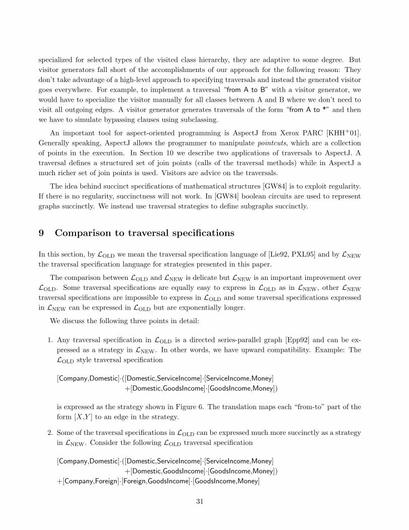
specialized for selected types of the visited class hierarchy, they are adaptive to some degree. But

visitor generators fall short of the accomplishments of our approach for the following reason: They

don’t take advantage of a high-level approach to specifying traversals and instead the generated visitor

goes everywhere. For example, to implement a traversal “from A to B” with a visitor generator, we

would have to specialize the visitor manually for all classes between A and B where we don’t need to

visit all outgoing edges. A visitor generator generates traversals of the form “from A to *” and then

we have to simulate bypassing clauses using subclassing.

An important tool for aspect-oriented programming is AspectJ from Xerox PARC [KHH+01].

Generally speaking, AspectJ allows the programmer to manipulate pointcuts, which are a collection

of points in the execution. In Section 10 we describe two applications of traversals to AspectJ. A

traversal defines a structured set of join points (calls of the traversal methods) while in AspectJ a

much richer set of join points is used. Visitors are advice on the traversals.

The idea behind succinct specifications of mathematical structures [GW84] is to exploit regularity.

If there is no regularity, succinctness will not work. In [GW84] boolean circuits are used to represent

graphs succinctly. We instead use traversal strategies to define subgraphs succinctly.

9 Comparison to traversal specifications

In this section, by LOLD we mean the traversal specification language of [Lie92, PXL95] and by LNEW

the traversal specification language for strategies presented in this paper.

The comparison between LOLD and LNEW is delicate but LNEW is an important improvement over

LOLD. Some traversal specifications are equally easy to express in LOLD as in LNEW, other LNEW

traversal specifications are impossible to express in LOLD and some traversal specifications expressed

in LNEW can be expressed in LOLD but are exponentially longer.

We discuss the following three points in detail:

1. Any traversal specification in LOLD is a directed series-parallel graph [Epp92] and can be ex-

pressed as a strategy in LNEW. In other words, we have upward compatibility. Example: The

LOLD style traversal specification

[Company,Domestic]·([Domestic,ServiceIncome]·[ServiceIncome,Money]

+[Domestic,GoodsIncome]·[GoodsIncome,Money])

is expressed as the strategy shown in Figure 6. The translation maps each “from-to” part of the

form [X,Y ] to an edge in the strategy.

2. Some of the traversal specifications in LOLD can be expressed much more succinctly as a strategy

in LNEW. Consider the following LOLD traversal specification

[Company,Domestic]·([Domestic,ServiceIncome]·[ServiceIncome,Money]

+[Domestic,GoodsIncome]·[GoodsIncome,Money])

+[Company,Foreign]·[Foreign,GoodsIncome]·[GoodsIncome,Money]

31

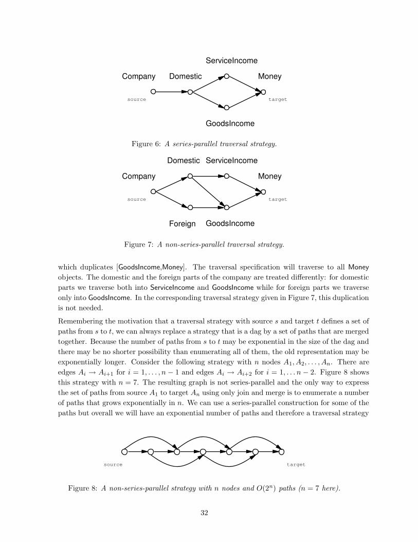
Company Domestic

ServiceIncome

GoodsIncome

Money

source target

Figure 6: A series-parallel traversal strategy.

Company

Domestic ServiceIncome

GoodsIncome

Money

source target

Foreign

Figure 7: A non-series-parallel traversal strategy.

which duplicates [GoodsIncome,Money]. The traversal specification will traverse to all Money

objects. The domestic and the foreign parts of the company are treated differently: for domestic

parts we traverse both into ServiceIncome and GoodsIncome while for foreign parts we traverse

only into GoodsIncome. In the corresponding traversal strategy given in Figure 7, this duplication

is not needed.

Remembering the motivation that a traversal strategy with source s and target t defines a set of

paths from s to t, we can always replace a strategy that is a dag by a set of paths that are merged

together. Because the number of paths from s to t may be exponential in the size of the dag and

there may be no shorter possibility than enumerating all of them, the old representation may be

exponentially longer. Consider the following strategy with n nodes A1, A2, . . . , An. There are

edges Ai → Ai+1 for i = 1, . . . , n − 1 and edges Ai → Ai+2 for i = 1, . . . n − 2. Figure 8 shows

this strategy with n = 7. The resulting graph is not series-parallel and the only way to express

the set of paths from source A1 to target An using only join and merge is to enumerate a number

of paths that grows exponentially in n. We can use a series-parallel construction for some of the

paths but overall we will have an exponential number of paths and therefore a traversal strategy

source target

Figure 8: A non-series-parallel strategy with n nodes and O(2n) paths (n = 7 here).

32

Flight City BusRoute

flights

cities

routes

cities*

*

*

*

Figure 9: Class graph for a transportation network.

source target

bypassing City

bypassing City

City BusRoute

Figure 10: A cyclic strategy.

that grows exponentially in n.

3. There are cyclic strategies (expressed in LNEW) which cannot be simulated by LOLD. Consider

the following traversal that cannot be simulated by a traversal specification in LOLD. For a given

city, we want to find all other cities reachable through zero or more bus routes. Consider this

specification in the context of the class graph in Figure 9. Using this class graph, we can start

at a city and follow paths of the form

〈City (routes BusRoute cities City)∗〉

to find all cities connected to it by bus routes only. We are not interested in the cities reachable

through flights. We can use the cyclic strategy shown in Figure 10, which selects the desired

City objects. But this cyclic strategy cannot be expressed by a series-parallel graph. We could

try:

from City bypassing City via BusRoute bypassing City to City

but this allows only cities reachable through an immediate bus route.

To summarize: the new language is exponentially more expressive in some cases and combined with

the exponential algorithmic improvement presented in this paper the new approach is considerably

more efficient than the old approach.

10 Applications of traversal strategies

This paper focuses on succinctly definining behavior for traversing through object graphs and on

efficient implementations of the traversals. However, our traversal theory (the expressive model and

the efficient algorithms) is applicable in a much wider context which we outline in this section.

The traversal theory relies on three layers of graphs: top, middle and bottom. The bottom layer

consists of trees that we want to traverse to select subtrees. Each bottom layer tree has a graph from

33

the middle layer associated with it that contains meta-information about the bottom layer tree. The

meta-information expresses that certain edges must or may exist. Each middle layer graph is associated

with at least one top layer graph. The top layer graph is basically a subgraph of the transitive closure

of the middle layer graph, decorated with additional information attached to the edges. The purpose

of the top layer graph is to define subtrees of the bottom layer graphs. In other words, when the

bottom layer graph is traversed, the top layer graph tells us at each node which outgoing edges to

traverse. The purpose of the middle layer graph is to act as an abstraction barrier between the top

and bottom layers. At the middle layer we program the specification given by the top layer and we

use the middle layer to reduce the search space.

The top layer graphs are an abstraction A of the associated middle layer graphs and the middle

layer graphs are an abstraction B of the associated bottom layer graphs. The abstractions A and

B, however, are different. Abstraction A involves the transitive closure and abstraction B involves

compatibility rules where relations at the middle layer imply relations at the bottom layer.

The traversal theory is also useful if we only use the top and the middle layer. In this case we are

interested in defining succinctly a set of paths in the graph in the middle layer. Sometimes we are not

interested in the details of the path set, just the subgraph or set of nodes that all those paths in the

set cover.

This general description fits many practical situations of which we mention a few, all of them of

interest to aspect-oriented programming.

• The standard application: Top: strategy graph, Middle: class graph, Bottom: object trees. The

strategy graph serves as a specification of a set of introductions of new traversal methods into

the class graph. This standard application is used extensively in DemeterJ and DAJ. DJ also

falls into this standard application, however, the traversal behavior is created at run-time by

specializing a generic traversal algorithm.

If we focus on the top and middle layer only, we need only our Traversal Graph Algorithm (TGA)

described in Section 5.1. One application of TGA is to use it to succinctly specify a set of types.

In AspectJ, type patterns could benefit from using strategies to specify a set of types succinctly.

A second application of TGA is the adapter generation approach by Bart Wydaeghe and Wim

Vanderperren [Wyd02, WV01, Van01]. The components that need to be connected might not

match and therefore an adapter has to be generated. The idea is that a traversal graph that is

constructed by TGA succinctly describes all possible adapters from which the programmer can

choose the most suitable one. The top layer graph represents the interactions of a high-level

component and the middle layer graph represents the interactions of a low-level component that

offers more detail than the other component asks for. The PacoSuite is a tool in which those

ideas have been successfully implemented and tested in an industrial context. The application

uses the full power of traversal strategies, including bypassing clauses and the name maps.

• The call graph application: Top: computational pattern, Middle: static call graph, Bottom: call

tree.

Static call graph: It is derived from the program source as follows. The nodes correspond

to methods and the edges to method invocation expressions (e.g. a.foo(b,c)) contained in the

34

methods. There are two types of methods: concrete and abstract. A concrete method has an

outgoing edge for every method the method calls or might call. Some of the outgoing edges

are marked required and others are marked optional. The required edges are to calls of other

methods that are reached unconditionally while optional edges correspond to calls that are

reached conditionally (some conditional statement might prevent the execution of the call; e.g.

an if, loop or switch statement). An abstract method has several outgoing edges marked as

virtual edges. Each leads to one of the method calls that might happen as a result of the virtual

method call. A static call graph has the shape of a class graph.

Dynamic call tree: It is a tree conforming to a static call graph. The nodes are calls of methods

(called join points) and the edges represent immediate method call nesting. Conformance means

that

1. the dynamic call graph can only contain instances of call sites appearing in the static call

graph;

2. the dynamic call graph can only contain edges prescribed by the static call graph;

3. if in the static call graph a required edge exits a call site then the edge must be in the

dynamic call graph; and

4. a call of a virtual method is not shown in the dynamic call graph; instead it shows the

concrete method that actually gets called.

A dynamic call tree has the shape of an object tree where call nodes correspond to object nodes

and immediately nested calls correspond to immediately nested objects.

As an example, consider the set of all method calls that might happen between a call to f and a

call to g. For each of those method calls we would like to print some information and we would

like to know how the join points are related. In other words, we want to know the structure

of the dynamic call tree between calls to f and calls to g. We would like to describe this slice

of the dynamic call tree as from pc1 to pc2, where pc1 = call(* f(..)) and pc2 = call(* g(..)).

(The pointcuts pc1 and pc2 specify that both f and g may return any type and both may have

arguments of any types.)

In a second example, we want to know for a thread and a resource type R all the read, write,

lock, and unlock calls that happen during the thread. Furthermore, we want to check that none

of those primitives call each other; for example, we want to disallow that write calls lock directly.

We consider four kinds of nodes in the static call graph corresponding to calls of the four

primitives.

pointcut read(): call(Object R.read(..));

pointcut write(): call(void R.write(..));

pointcut lock(): call(void R.lock(..));

pointcut unlock(): call(void R.unlock(..));

pointcut primitive(): read() || write() || lock() || unlock();

The pointcut start contains a node in the static call graph where the computation starts. We

consider the following two strategies:

35

s1 = from start() to primitive()

s2 = from start() bypassing primitive() to primitive()

(Note that bypassing a node does not bypass that node if it is a start or end point.)

The primitives don’t call each other iff, for the given static call graph, s1 = s2 (more precisely,

if the traversal graphs determined by the two strategies are equal). This second example is

interesting because it shows that strategies are useful to formulate architectural properties of

call graphs at a high level of abstraction.

Finally, we present a use of the call graph application in serialization/marshalling which is a very

common example of object traversal. A serializer is a tool transforming partial graphs of objects into a

stream of bytes. In [Lop96], simple traversal directives (which are single edge strategy graphs) are used

to specify which parts of a compound object should be copied and which should be passed by reference

when using remote method invocations. Our work on traversals is useful to current work in object

serialization [PHN00, Bar97, HH19] in the following way: A common concern in serialization is how to

generate serialization code with minimal impact on the code size of the application, or alternatively,

how to arrange dynamic traversal with minimal run-time impact. We address this concern by showing

in Section 6 that if the traversal methods are not generated carefully from a partial object specification

(as described in this paper), one might end up with exponential code size. Our implementation of DJ

shows how to arrange dynamic traversal and the DemeterJ and DAJ implementations show how to

generate efficient code efficiently. We also show a general way to specify partial objects. This paper

solves the problem by using a marshalling language (our traversal strategy language) to specify partial

object graphs.

11 Experience and empirical evidence

The algorithms described in this paper have been used extensively in our tools and tools developed by

others. Surprisingly, neither the exponential algorithmic improvements nor the more general model

seem to be so important for the applications where we used traversals so far. The earlier compilation

algorithm, called the Xiao-algorithm, described in [PXL95] worked very well in practice and the expo-

nentially bad cases described in this paper did not seem to appear in practice. But the Xiao-algorithm

was challenging to program and occasionally required the programmer to rewrite the traversal speci-

fications in case the algorithm could not handle the combination of current strategy and class graph.

The threat of slow performance and the lack of generality made us to switch to the algorithm described

in this paper.

The remark that the Xiao algorithm worked well in practice is supported by the following statistics

for DemeterJ, which is implemented in its own language. The entire tool uses 236 strategies of which

only 32 strategies are multi-edge. This gives an average of 1.144 edges per strategy. The largest

strategy has 4 edges. (It should be remarked that in a redesign of DemeterJ the average would be

higher because, due to tool limitations, some strategies make use of bypassing instead of using more

strategy edges.) Because strategies are small in DemeterJ, the efficiency of our new algorithm is not so

36

important for the DemeterJ application. The complete set of strategies used in DemeterJ are available

in [Orlb].

Traversal strategies are usually much smaller than the corresponding traversal graph. Mitchell

Wand and Pengcheng Wu have done some statistics collecting by implementing and applying another

traversal generating algorithm [LW01] with the same traversal strategy syntax as ours on the traversals

used in DemeterJ’s generate package source files, which have 80 traversals in total. Table 1 lists the

distribution of the ratio of the length of traversal methods call path vs. the length of strategy for the

80 traversals. As you can see from the table, of the 80 traversals, over 40 traversals have ratios bigger

than 4, which reflects the size difference between traversal strategy and traversal graph. More detailed

data are available in [WW].

Range of the ratios [0,2) [2,4) [4,6) [6,8) [8,10) [10,12) [12,∞)

Number of traversals 11 26 19 13 4 5 2

Table 1: Distribution of the ratio of the length of call path vs. the length of strategy.

An industrial project at Verizon which uses DemeterJ was presented at the first International

Conference on Aspect-Oriented Software Development (AOSD) in April 2002 [BM02] as an example

of successful use of AOSD technology in industry. The traversal specifications worked very well in this

project over a period of five years. The evolution history of the project is available on the web [Bla02].

Further evidence that traversal strategies work can be obtained from the successful use of the

Demeter/C++ system [Lie96]. Demeter/C++ was used at Northeastern University from 1992 to 1996,

and in other places, including at Citibank, IBM, Bell Northern Research, Credit Suisse and at several

universities. See [Lieb] for an extensive description of the system and relevant references. The first

version of Demeter allowed only very simple traversals (corresponding to single-edge strategy graphs

with bypassing clauses), and generated code in C++. Demeter/C++ compiles traversals which can be

described by a series-parallel graph, but only for a restricted set of class graph/strategy combinations.

Hewlett-Packard has reported a positive experience in using the traversal/visitor style of program-

ming for writing installation software for the HP printers family [Liea].

Finally, another piece of empirical evidence is that the Law of Demeter [LH89] is still considered

to be a good idea [HT00]. However, writing all of the methods needed to forward calls is tedious

and error prone. Traversal strategies may be used to specify the forwarding calls at a high level of

abstraction.

12 Conclusion

Traversals are fundamental to object-oriented programming and programming in general. In order to

process an object we need to traverse through a part of it and perform appropriate actions during

the traversal. The importance of traversals of object structure is well recognized in the literature.

For example, the Visitor design pattern [GHJV95] and its variants [Vli95, Vli96, JP98] attest to this

fact. We believe that the notion of strategies is a significant contribution to software developers—both

37

by providing a more intuitive and conceptually simpler programming model, and by automating the

frequent-and-tedious task of programming traversals.

In this paper we have extended the state of knowledge regarding traversals by providing a general

definition as well as an efficient implementation and a working prototype. We improve on all previous

implementations and at the same time we present a model that is more general than previous traversal

models. In addition, the lower bound result improves the understanding of the inherent properties of

run-time traversals, whose implementation has been notoriously tricky.

U.S. patent 5,946,490 covers the algorithms in this paper.

Acknowledgments

We wish to thank Dean Allemang, James Deikun, Lars Hansen, Jens Palsberg, Kedar Patankar, Salil

Pradhan, Johan Ovlinger, Binoy Samuel, Benedikt Schulz, and Mitch Wand for numerous discussions

and suggestions. Special thanks are due to Michal Young, for bringing [ASU86] to our attention.

Many thanks to the ACM reviewers for their detailed and helpful feedback.

38

References

[ASU86] Alfred V. Aho, Ravi Sethi, and Jeff D. Ullman. Compilers—Principles, Techniques, and

Tools, pages 126–127. Addison-Wesley, 1986. (Algorithm 3.4).

[Bar97] A. Bartoli. A novel approach to marshalling. Software–Practice and Experience, 27(1):63–

85, January 1997.

[Bla02] Luis Blando. Mission Critical Verizon Project Using DemeterJ. Technical report, Verizon,

2002. http://www.ccs.neu.edu/research/demeter/evaluation/gte-labs/.

[BM02] Luis Blando and Nosherwan Minwalla. Commercial AOSD Deployment in Action: Five

Years and Counting. In Gregor Kiczales, editor, First International Conference on Aspect-

Oriented Software Development, Enschede, The Netherlands, 2002.

[BPe98] Tim Bray, Jean Paoli, and C. M. Sperberg-McQueen (eds.). Extensible Markup Language.

http://www.w3.org/TR/REC-XML, February 1998.

[BRJ99] Grady Booch, James Rumbaugh, and Ivar Jacobson. The Unified Modeling Language User

Guide. Object Technology Series. Addison Wesley, 1999. ISBN 0-201-57168-4.

[BV01] M. Bravenboer and E. Visser. Guiding visitors: Separating navigation from computation.

Technical report, Institute of Information and Computing Sciences, Utrecht University,

2001.

[Ce99] James Clark and Steve DeRose (eds.). XML Path Language (XPath), version 1.0.

http://www.w3.org/TR/XPath, November 1999.

[CI84] Robert D. Cameron and M. Robert Ito. Grammar-based definition of metaprogramming

systems. ACM Transactions on Programming Languages and Systems, 6(1):20–54, January

1984.

[Con] W3 Consortium. XML schema home page. http://www.w3.org/XML/Schema/. Continu-

ously updated.

[EFB01] Tzilla Elrad, Robert Filman, and Atef Bader. Aspect-Oriented Programming. Communi-

cations of the ACM, 44(10):28–97, 2001.

[Epp92] David Eppstein. Parallel recognition of series-parallel graphs. Information and Computa-

tion, 98(1):41–55, 1992.

[FMY92] R. Farrow, T.J. Marlow, and D.M. Yellin. Composable Attribute Grammars: Support for

modularity in translator design and implementation. In ACM Symposium on Principles of

Programming Languages, pages 223–234. ACM Press, 1992.

[GHJV95] Erich Gamma, Richard Helm, Ralph Johnson, and John Vlissides. Design Patterns: Ele-

ments of Reusable Object-Oriented Software. Addison-Wesley, 1995.

39

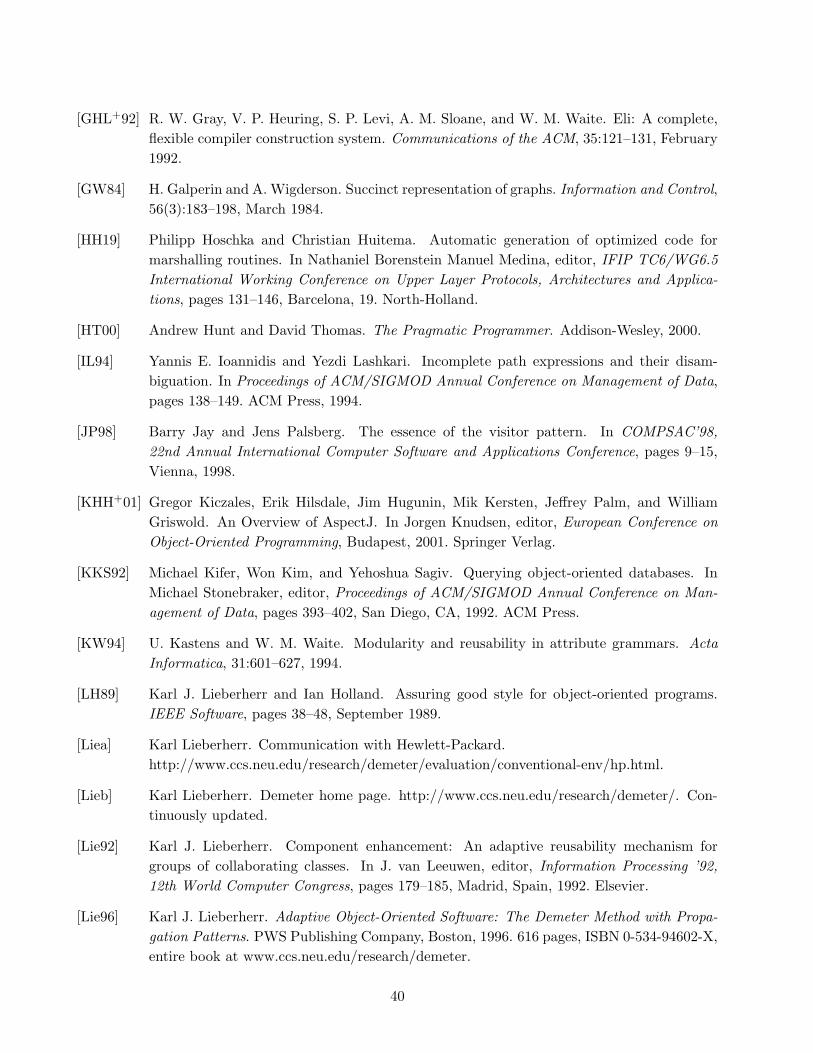
[GHL+92] R. W. Gray, V. P. Heuring, S. P. Levi, A. M. Sloane, and W. M. Waite. Eli: A complete,

flexible compiler construction system. Communications of the ACM, 35:121–131, February

1992.

[GW84] H. Galperin and A. Wigderson. Succinct representation of graphs. Information and Control,

56(3):183–198, March 1984.

[HH19] Philipp Hoschka and Christian Huitema. Automatic generation of optimized code for

marshalling routines. In Nathaniel Borenstein Manuel Medina, editor, IFIP TC6/WG6.5

International Working Conference on Upper Layer Protocols, Architectures and Applica-

tions, pages 131–146, Barcelona, 19. North-Holland.

[HT00] Andrew Hunt and David Thomas. The Pragmatic Programmer. Addison-Wesley, 2000.

[IL94] Yannis E. Ioannidis and Yezdi Lashkari. Incomplete path expressions and their disam-

biguation. In Proceedings of ACM/SIGMOD Annual Conference on Management of Data,

pages 138–149. ACM Press, 1994.

[JP98] Barry Jay and Jens Palsberg. The essence of the visitor pattern. In COMPSAC’98,

22nd Annual International Computer Software and Applications Conference, pages 9–15,

Vienna, 1998.

[KHH+01] Gregor Kiczales, Erik Hilsdale, Jim Hugunin, Mik Kersten, Jeffrey Palm, and William

Griswold. An Overview of AspectJ. In Jorgen Knudsen, editor, European Conference on

Object-Oriented Programming, Budapest, 2001. Springer Verlag.

[KKS92] Michael Kifer, Won Kim, and Yehoshua Sagiv. Querying object-oriented databases. In

Michael Stonebraker, editor, Proceedings of ACM/SIGMOD Annual Conference on Man-

agement of Data, pages 393–402, San Diego, CA, 1992. ACM Press.

[KW94] U. Kastens and W. M. Waite. Modularity and reusability in attribute grammars. Acta

Informatica, 31:601–627, 1994.

[LH89] Karl J. Lieberherr and Ian Holland. Assuring good style for object-oriented programs.

IEEE Software, pages 38–48, September 1989.

[Liea] Karl Lieberherr. Communication with Hewlett-Packard.

http://www.ccs.neu.edu/research/demeter/evaluation/conventional-env/hp.html.

[Lieb] Karl Lieberherr. Demeter home page. http://www.ccs.neu.edu/research/demeter/. Con-

tinuously updated.

[Lie92] Karl J. Lieberherr. Component enhancement: An adaptive reusability mechanism for

groups of collaborating classes. In J. van Leeuwen, editor, Information Processing ’92,

12th World Computer Congress, pages 179–185, Madrid, Spain, 1992. Elsevier.

[Lie96] Karl J. Lieberherr. Adaptive Object-Oriented Software: The Demeter Method with Propa-

gation Patterns. PWS Publishing Company, Boston, 1996. 616 pages, ISBN 0-534-94602-X,

entire book at www.ccs.neu.edu/research/demeter.

40

[LO97] Karl J. Lieberherr and Doug Orleans. Preventive program maintenance in Demeter/Java

(research demonstration). In International Conference on Software Engineering, pages

604–605, Boston, MA, 1997. ACM Press.

[LOO01] Karl Lieberherr, Doug Orleans, and Johan Ovlinger. Aspect-Oriented Programming with

Adaptive Methods. Communications of the ACM, 44(10):39–41, 2001.

[Lop96] Cristina Videira Lopes. Adaptive parameter passing. In 2nd International Symposium on

Object Technologies for Advanced Software, pages 118–136, Kanazawa, Japan, March 1996.

Springer-Verlag.

[LSX94] Karl J. Lieberherr, Ignacio Silva-Lepe, and Cun Xiao. Adaptive object-oriented program-

ming using graph-based customization. Communications of the ACM, 37(5):94–101, May

1994.

[LVV03] Ralf Lammel, Eelco Visser, and Joost Visser. Strategic programming meets adaptive

programming. In Proc. of AOSD’03. ACM Press, 2003.

[LW01] Karl Lieberherr and Mitchell Wand. Traversal semantics in object graphs. Technical Report

NU-CCS-2001-05, Northeastern University, May 2001.

[MS93] Victor M. Markowitz and Arie Shoshani. Object queries over relational databases: Lan-

guage, implementation, and application. In 9th International Conference on Data Engi-

neering, pages 71–80. IEEE Press, 1993.

[MS01] Bob McWhirter and James Strachan. Extensible Markup Language. http://jaxen.org/,

2001.

[NS88] Erich J. Neuhold and Michael Schrefl. Dynamic derivation of personalized views. In

Proceedings of the 14th VLDB Conference, pages 183–194, 1988.

[OL01] Doug Orleans and Karl Lieberherr. DJ: Dynamic Adaptive Programming in Java. In

Reflection 2001: Meta-level Architectures and Separation of Crosscutting Concerns , Kyoto,

Japan, September 2001. Springer Verlag. 8 pages.

[Orla] Doug Orleans. DAJ home page. http://daj.sf.net/. Continuously updated.

[Orlb] Doug Orleans. DemeterJ Strategy Statistics.

http://www.ccs.neu.edu/research/demeter/DemeterJ/strategy-usage-in-DemeterJ.txt.

[PHN00] M. Phillipsen, B. Haumacher, and C. Nester. More Efficient Serialization and RMI for

Java. Concurrency: Practice and Experience, 12(7):495–518, May 2000.

[Pol49] George Polya. How To Solve It. Princeton University Press, 1949.

[PPL97] Jens Palsberg, Boaz Patt-Shamir, and Karl Lieberherr. A new approach to compiling

adaptive programs. Science of Computer Programming, 29(3):303–326, 1997.

41

[PXL95] Jens Palsberg, Cun Xiao, and Karl Lieberherr. Efficient implementation of adaptive soft-

ware. ACM Transactions on Programming Languages and Systems, 17(2):264–292, March

1995.

[SD01] Kurt Stirewalt and Laura K. Dillon. Generation of visitor components that implement

program transformations. In ACM SIGSOFT Symposium on Software Reusability, pages

86–94, 2001.

[Sma] Yannis Smaragdakis. Personal communication. 1997.

[SPL96] Linda M. Seiter, Jens Palsberg, and Karl J. Lieberherr. Evolution of Object Behavior

using Context Relations. In David Garlan, editor, Symposium on Foundations of Software

Engineering, SIGSOFT, pages 46–57, San Francisco, 1996. ACM Press (SIGSOFT).

[SPL98] Linda M. Seiter, Jens Palsberg, and Karl J. Lieberherr. Evolution of Object Behavior using

Context Relations. IEEE Transactions on Software Engineering, 24(1):79–92, January

1998.

[Sun02] John Sung. Aspectual Concepts. Technical Report NU-CCS-02-06, Northeastern Univer-

sity, June 2002. Master’s Thesis, http://www.ccs.neu.edu/home/lieber/theses-index.html.

[Van01] Wim Vanderperren. Applying aspect-oriented programming ideas in a component based

context: Composition adapters. In GCSE, Erfurt, Germany, 2001.

[VdBV93] Jan Van den Bussche and Gottfried Vossen. An extension of path expressions to simplify

navigation in object-oriented queries. In Stefano Ceri, Katsumi Tanaka, and Shalom Tsur,

editors, Deductive and Object-Oriented Databases, pages 267–282, Phoenix, Arizona, 1993.

Springer Verlag, Lecture Notes in CS, No. 760.

[Vli95] John Vlissides. Visiting rights. C++ Report, September 1995.

[Vli96] John Vlissides. The Trouble with Observer. C++ Report, September 1996.

[WG84] William Waite and Gerhard Goos. Compiler Construction. Springer Verlag, 1984.

[Woo96] Bobby Woolf. The Null Object pattern. In Pattern Languages of Program Design, 1996.

[WV01] Bart Wydaeghe and Wim Vanderperren. Towards a new component composition process.

In ECBS, Washington, April 2001.

[WW] Mitch Wand and Pengcheng Wu. Part of the Statistics of Traversing Methods Generated

For DemeterJ Source Code. http://www.ccs.neu.edu/home/wupc/statistics/statistics.htm.

[Wyd02] Bart Wydaeghe. PACOSUITE: Component Composition Based on Composition Patterns

and Usage Scenarios. PhD thesis, Free University of Brussels, 2002.

42

l

b

c d

e f

m

l

b

c d

e f

ml m

l

b

c d

e f

ml m

a l b

c d

e f

m

aa’

l la aa’ a’

A B C D

Figure 11: An example of class graph simplification. A: the original class graph. Concrete classes are

depicted as squares, and abstract classes are hexagons. Reference edges are regular, and subclass edges

are heavy. B: after step 1. C: after step 2. D: after step 3.

APPENDICES

A Class graph Simplification

In this appendix we prove Proposition 2.1. For the convenience of the reader, we reproduce it below.

Proposition 2.1. Let G = (V, E) be an arbitrary class graph. Then there exists a simple class graph

Simplify(G) = (V ′, E′) such that an object graph Ω is an instance of G if and only if Ω is an instance

of Simplify(G). Moreover, |V ′| = O(|V |) and |E′| = O(|E|2).

The proposition is proven by the following transformation algorithm (see example in Figure 11).

1. For each concrete class v ∈ V with an outgoing subclass edge v→ u ∈ E, add a new abstract

node v′ into V , along with the following changes of the edge set:

• Divert all edges coming into v to end at v′. That is,

E ← E ∪

ul→ v′ | u

l→ v ∈ E

\

ul→ v | u

l→ v ∈ E

• Divert all subclass edges going out from v to originate at v′. That is,

E ← E ∪

v′→ u | v

→ u ∈ E

\

v→ u | v

→ u

• Make v a subclass of v′:

E ← E ∪

v′→ v

When this step is completed, no concrete class has subclass edges going out from it.

2. For each concrete class v: add edges so that the set of edges going out from v is exactly the

induced edges of v. Then, delete all reference edges going out from abstract classes.

3. Contract long inheritance chains. For each abstract class v: find all concrete classes u which can

be reached from v using subclass edges only, and add a subclass edge v→ u if one does not exist

already. Finally, delete all subclass edges leading to abstract classes.

43

Informally, Step 1 decouples the sub-classing role from concrete classes by introducing an additional

abstract class for each class which has both subclass and reference edges going out from it.

Step 2 unfolds inherited reference edges by pushing them down the subclass hierarchy. This can

be done efficiently by traversing the subclass edges in a top-down fashion, starting with nodes with no

subclass edges coming into them, and “collecting” reference edges as we go down. Details are omitted.

Step 3 can be viewed as taking the transitive (non-reflexive) closure of the subclass relation. This

step can be done in parallel with Step 2.

For the bound on the size of the resulting graph, note first that only Step 1 may change the

number of nodes by at most doubling it. Next, note that since Steps 2 and 3 do not change the

connectivity structure of the graph, we can deal with each connected component separately. Consider

such a component with n nodes. Since it is connected, there are at least n−1 nodes in the component

before Steps 2 and 3. Since these steps do not introduce nodes or parallel edges, they may introduce

at most O(n2) new edges. We may therefore conclude that the number of nodes in Simplify(G) is at

most doubled and the number of edges is at most squared.

B Target language for static compilation

Static traversal compilers compile strategies and class graphs into an object-oriented program where

the sequence of methods invoked by an object depends only on the object structure and the method

name (no parameter passing is allowed). Formally, the language is defined as follows.

A program in the target language is a partial function which maps a class name and a method name

to a method. A method is a tuple of the form 〈l1.m1, . . . , ln.mn〉, where l1 . . . ln ∈ L and m1 . . .mn

are method names. When invoked, such a method executes by invoking li.mi in order. We distinguish

two kinds of methods: visiting and non-visiting, prescribed by a predicate visit defined on the set of

method names.

An invocation of a program is defined as follows. If Ω is an object graph, o a node in Ω, m a

method name, P a program in the target language, and H a sequence of objects, then the judgment

Ω `c o : m : P H

means that when sending the message m to o, we get a traversal of the object graph Ω starting in

o so that H is the traversal history. Formally, this holds when the judgment is derivable using the

following rules:

Ω `c oi : mi : P Hi ∀i ∈ 1..n

Ω `c o : m : P o ·H1 · ... ·Hn

if P(Class(o), m) = 〈l1.m1 . . . ln.mn〉, and

visit(m), and oli→ oi is in Ω for all i ∈ 1..n.

and

Ω `c oi : mi : P Hi ∀i ∈ 1..n

Ω `c o : m : P H1 · ... ·Hn

if P(Class(o), m) = 〈l1.m1 . . . ln.mn〉, and

¬visit(m), and oli→ oi is in Ω for all i ∈ 1..n.

The label c of the turnstile indicates “code”. Intuitively, the rule says that when sending the message

m to o, we check if o understands the message, and if so, we invoke the method. The object o is added

44

to the traversal history only if visit(m) is true. Notice that for n = 0, the rule is an axiom; in the case

that visit(m) is true, it is simply

Ω `c o : m : P oif P(Class(o), m) = 〈〉

and if visit(m) is false, then it is

Ω `c o : m : P εif P(Class(o), m) = 〈〉,

where ε denotes the empty history.

Given a program in the target language, it is straightforward to generate, for example, a C++ or a

Java program.

45