Traveling-Wave Modeling of Semiconductor Lasers and Amplifiers · 2005-11-15 · Traveling-Wave Modeling of Semiconductor Lasers and Amplifiers Hans-Jürgen Wünsche Humboldt University

Traveling-Wave Modeling of Semiconductor Lasers and Amplifiers

Hans-Jürgen Wünsche Humboldt University of Berlin, Germany

Mindaugas Radziunas Weierstrass Institute for Applied Analysis and Stochastics, Berlin, Germany

outline

NUSOD05 Tutorial MB1 Wünsche/Radziunas Traveling-Wave Modeling: 2

introductionbasic traveling-wave (TW) modeladvanced aspectsexamplaric simulationsmode analysismode approximationsbifurcation analysissummary

chapter 1: introduction


what is traveling wave modeling?relations to other model classesadvantagesorigins

what is traveling wave modeling ?


devices with good waveguides

z: 102 µm

x: 1 µm

y: 1 µm transverse-longitudinalseparation possible

subjects of TW modeling: optical amplitude

inversion density

relation to other model classes


• sophisticated:

Hess O, ... Prog Quant Electr 20, 85 (96)

• TW models:

• rate equations:

advantages of TW models


intermediate level of complexity: as fast as rate equationsbut more flexible and detailed

time domain model: stationary, small & large signal properties

covers many types of devices:

• semiconductor optical amplifier (SOA)• standard edge emitting laser• multisection laser• ring laser configurations• coupled laser structures

but not: tapered structures, VCSELs, LEDs, ...

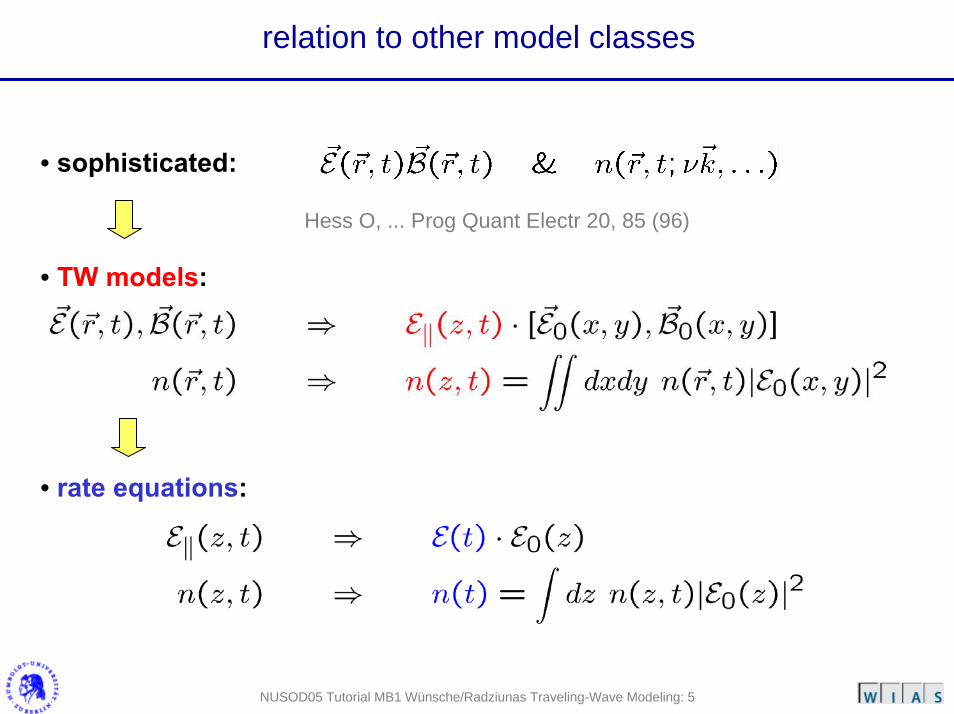
origins of traveling wave modeling


• Maxwell-Bloch equations prototype of TW modelsArecchi & Bonifaci, JQE 1,169 (65)Theory of optical maser amplifiers

TU of Denmark• small-signal laser modelingTromborg B, ... JQE 23, 1875 (87)

Nottingham: transmission-line model• large-signal laser modelingLowery AJ, IEE Proc J 134, 281 (87)

Gent: CLADISSMorthier G, ... JQE 26, 1728 (90)

Cambridge Carroll JE ... JQE 28, 604 (92)

Berlin Bandelow U, ... PTL 5, 1176 (93)

chapter 2: basic traveling-wave model


let us understand the equations

• ingredients from waveguiding• slowly varying amplitudes• propagation equations• carrier rate equations

ingredients from waveguiding


relativerelative z

Henry factor

gain

n=const.reference reference

supposed to be known:

higher ordercontributions

fundamentaldispersion

basic model:

losses

slowly varying amplitudes


z

n=const.

propagation equation for forward traveling wave

backward wave: analogouskeeps valid for

propagation equations: distributed feedback


z grating with period

2 equations coupled by

reflections at grating couple forward-backward

choosing k0=π/Λ yields

boundary conditions


example: device facet0

z

R

general junction at z0:

may connect multiple incoming waveguides uwith multiple outgoing waveguides v

very flexible !

carrier rate equations


averaging in appropriate subsections s:

...n1(t) n2(t) n3(t) n4(t)

pumprate

spontreco stimulated recombination

backgroundlosses in β

basic model:

summary of basic equations


optical TW equation

carrier rate equations:

waveguide propagation model: propagation constantrelative to k0

taken at ω0

chapter 3: advanced aspects


some important extensions of the basic model

• nonlinear gain saturation• gain dispersion• spontaneous emission• current redistribution• few words on numerics

nonlinear gain saturation


gain decreases with optical intensity |E|2

possible reasons: redistribution of carriers• in energy (carrier heating,

spectral hole burning)• in transverse space (transverse spatial hole burning)effective refractive index is much less influenced

model:

... Schimpe R, APL 60, 2720 (92)also tutorial Koch (MA2)

typical order of magnitude: ε ≈ 1 W -1 ⇒ small effect

but important for dynamics, e.g. damping of relaxation oscillations,

four-wave mixing

Petermann K, chapter 5 inLaser diode modulation and noise,Kluwer 1988

gain dispersion


gain

ω

30-100 nmgain dispersion:

although gain bandwidth >> width of laser spectrum,gain disperision is important for• mode selection in FP & index coupled DFB lasers• avoiding unphysical spurious solutions

(high frequency components)

treating gain dispersion in TW models


basic model

• numerical temporal filtering

• additional polarization equation(simplest: Lorentzian line shape)

• spatial digital filtering

main methods:

Ning... JQE 33, 1543 (97)Bandelow… JQE 37, 183 (01)

Carroll JE, … DFB lasersIEE Publishing (98)

Kolesik & MoloneyJQE 37, 936 (01)

inclusion of gain dispersion : operator in time domain models

spontaneous emission


spontaneous emission = quantum-optical effectsemiclassical approximation by spatially uncorrelated white-noise:

more details in:

Langevin Equ.

Henry CH & Kazarinov RFquantum noise in photonics Rev Mod Phys 68, 801 (96)Carroll JE, … DFB lasersIEE Publishing (98)

current redistribution


metallic contact = equipotential

intensity |E|2 nonuniformstimulated reco nonuniforminversion n nonuniform= longitudinal spatial hole burning

(LSHB)

injection rate J nonuniform= current redistribution,

counteracts LSHBmodel:

Champagne Y... JAP 72, 2110 (92)Eliseev PG... JSTQE 3, 499 (97)

few words on traveling-wave numerics


finite difference schemes approximating fields Ψ(z,t) along characteristic lines • basics with numerical filtering:

J. Carroll ... DFB lasers, Chapter 7, IEE & SPIE 1998

• with polarization equations:M. Radziunas ... Chapter 5 in ``Optoelectronic Devices ...'', J. Piprek ed., Springer, 2005

further approaches:

• transfer matrix method Zhang LM, JQE 28, 604 (92)Marcenac DD, PhD Thesis,Cambridge 93

• split step method Kim BS … JQE 36, 787 (00)

• transmission line approach Lowery AJ, IEE Proc J 134, 281 (87)

chapter 4: examplaric simulations


TW modeling on work - settle back and enjoy!

• semiconductor optical amplifier (SOA)• simple Fabry-Perot (FP) laser• simple index-coupled distributed feedback (DFB) laser• small signal modulation response• large signal modulation• mode locked laser• self-pulsating multi-section DFB laser• locking to external bit streams• ring laser

semiconductor optical amplifier (SOA): idle running


z

ASEASE• ideal SOA: zero facet reflectivities • idle running: without optical injection• only radiation source: spontaneous emission• device emits amplified spontaneous emission (ASE)

TW modeling

components & measurements: HHI Berlin

experiment

TW model well describesASE spectra of idle SOA

wavelength (nm)

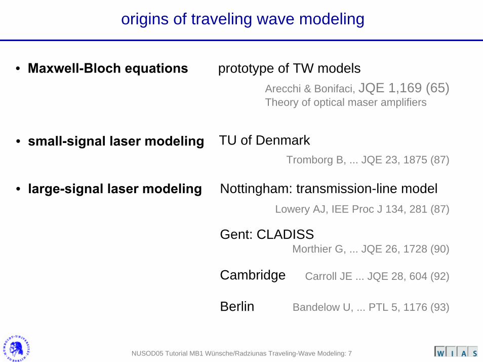
SOA: four wave mixing (FWM)


λ2λ1

experiment (HHI)

experiment: two waves are injected withdifferent wavelengths

SOA

λ1spectrum?

λ2wavelength (nm)

TW model inherently containsthe generation of satellite wavesby four wave mixing

TW modeling


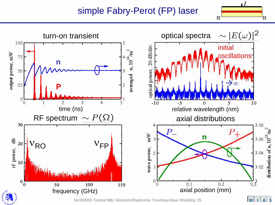
RRsimple Fabry-Perot (FP) laser

axial distributions

n

optical spectra

t ∞

initialoscillations

turn-on transient

n

P

RF spectrum

νRO νFP

time (ns)

frequency (GHz)

relative wavelength (nm)

axial position (mm)


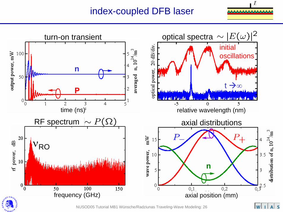
index-coupled DFB laser

optical spectrainitialoscillations

turn-on transient

n

P t ∞

axial distributions

n

RF spectrum

νRO

time (ns)

frequency (GHz)

relative wavelength (nm)

axial position (mm)

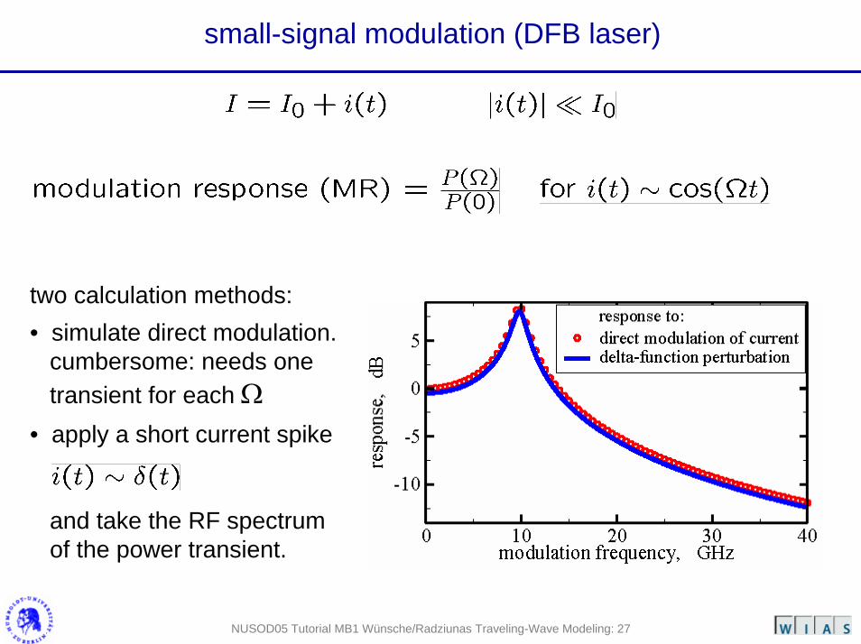
small-signal modulation (DFB laser)


two calculation methods: • simulate direct modulation.

cumbersome: needs onetransient for each Ω

• apply a short current spike

and take the RF spectrumof the power transient.

large signal modulation


DFB+EC laser: direct modulation with 40 Gb/s NRZ PRBS

eye histogram

M. Radziunas: talk TuD2 Tuesday afternoon

self-pulsating multisection laser


t/ps=

time (ps)

locking of self-pulsations to external signals


fext

dashed: injected frequencies fext

blue:the pulsation locks to the externalfrequency

red:the pulsation does not lockbut shows repeated phase slips

monolithitic mode-locked laser


RR

SA

benchmark device of COST 288

optical spectra: many locked modestransient pulse sequence

time (ps) relative wavelength (nm)

RF spectrum: SNR sampled pulses (eye)

frequency (GHz) time (ps)

ring laser with extended cavity


optical switching betweentwo stable cw states

S. Zhang ..., IEEE JSTQE 10, 2004

chapter 5: mode analysis


optical fields can be represented by modes in time and frequency domains

• mode definition• how to compute modes• meaning of complex mode frequencies• how modes depend on inversion• mode expansion of the field• examples

motivation


Wünsche .... J Sel Top QE 9 857 (03)

-2 -1 0 1

modes

inte

nsity

(10d

B/d

iv )

FWMFWM

rel. wavelength ( nm )

optical modes = natural oscillations of the laser cavity• they govern the optical spectra• but not all spectral lines are modes

Marcuse .... JQE 19 1397 (83)

multimode rate equations

• modes play an important rolein laser dynamics

• modal intensities are subjectof multimode rate equations

• how to treat modes in thetraveling-wave approach?

mode definition


full TW equation: +b.c.

mode function

mode equation: +b.c.

mode frequency (complex)

facet reflectivitiescharacteristic equ.:

overall transfer matrix

how to compute modes


FP laser: analytic solution

Other lasers: homotopy method, starting from FP

M. Aubry, Homotopy Theory and Models Boston, MA:Birkhäuser, 1995.

meaning of complex mode frequencies Ωm


2 Im Ω

full mode field

intensity

DFB

2 Im Ωm = modal decay rateRe Ωm = mode frequency

⇔ wavelength

how modes depend on inversion


simple laser

5ps decay

solitary DFB

compound laser3-section DFB

mode expansion of the optical field


mode functions form basis of the Hilbert spaceoptical field can be expanded in a mode series

rigorous formulations:J. Rehberg ... ZAMM 77, 75 (97)J. Sieber, PhD Thesis, HU Berlin (01)

adjoint mode Hilbert space scalar product

such expansion is possible for any choosen β

the instantaneous modes adapt themselves adiabaticallyto slow changes of the optical cavity.

examples


turn-on spiking FP laserstable two-mode pulsation

mode expansion allows:• to identify dominant modes• to identify which peaks of the optical spectra belong to modes• to interprete properly nontrivial transients of the field

chapter 6: finite dimensional mode approximations


field projection onto moving subspaces spanned by few instantaneous modes

• amplitude equations• the simple case of solitary lasers• restriction to essential modes • precision of mode approximations • math foundation: center manifold theorem

amplitude equations


moving modes:

how evolve the mode amplitudes? H. Wenzel ... IEEE JQE 32, 69 (96)

mode coupling factors

spontaneous emissioninto mode k

the simple case of solitary lasers


=0independent of t

↓ (drop noise for simplicity)

↓noncoupled rate equationsfor photon number Sk ~ |fk|2

Marcuse .... JQE 19 1397 (83)

mode coupling by Kkl is a specific effect of compound lasers

restriction to essential modes


|fk|2: only few modeswith noticeableamplitude

restriction to these essental modes yields closed set of ODE:

t ∞

precision of mode approximations


most relevant modes dependence on number q of modes

2 3>3 circles:simulation

time (ns)

mathematical foundation: center manifold theorem


consider the TW model

It holds:• only finitely many eigenvalues iΩ (n) of iH(n) are critical

(close to imaginary axis or with positive real part).• All they have finite algebraic multiplicity• it exists an exponentially attracting smooth invariant manifold

J. Sieber, PhD Thesis, HU Berlin, 2001

asymptotic motion on a finite dimensional center manifold

chapter 7: bifurcation analysis


an elegant way to understand the inherent nonlinearities

• what is a bifurcation? • why bifurcation analysis?• how doing bifurcation analysis of TW models?• example• live demonstration

what is a bifurcation?


a famous old example:river Orinoke splits in two arms

in our context:• qualitative change of a solution

under smooth variation of a control parameter

• border in parameter space betweenregions of different behaviour

drawing by Humboldt, fromhttp://www.uni-potsdam.de/u/romanistik/humboldt/hin/leitner-HINIII.htm

why bifurcation analysis?


How do operation regimes depend on parameters?You can scan parameters by simulation, but:• this procedure is mostly very laborious• possible multistabilities (hysteresis) require

to check different initial conditions.

Bifurcation analysis is more elegant: • it calculates only the border lines between regimes• it allows to classify the different bifurcations

B. Krauskopf in ``Fundamental issues of Nonlinear Laser Dynamics'', AIP 2000

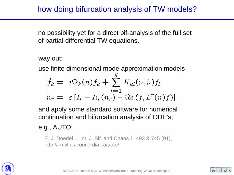
how doing bifurcation analysis of TW models?


no possibility yet for a direct bif-analysis of the full setof partial-differential TW equations.

way out: use finite dimensional mode approximation models

and apply some standard software for numerical continuation and bifurcation analysis of ODE's,e.g., AUTO:

E. J. Doedel ... Int. J. Bif. and Chaos 1, 493 & 745 (91), http://cmvl.cs.concordia.ca/auto/

example


live demonstration: DFB laser with integrated external cavity


summary of the tutorial


traveling-wave modeling• bases on transverse-longitudinal separation• resolves longitudinal coordinate z and time t• is the method of choice for compound-cavity devices• but is useful for simpler configurations, too.

more information on the used simulation tool LDSL:http://www.wias-berlin.de/software/ldsl/

one-parameter bifurcation diagrams


Documents

Traveling-Wave Modeling of Semiconductor Lasers and Amplifiers · 2005-11-15 · Traveling-Wave Modeling of Semiconductor Lasers and Amplifiers Hans-Jürgen Wünsche Humboldt University