1

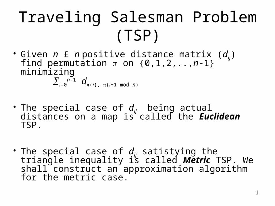
Traveling Salesman Problem (TSP)

• Given n £ n positive distance matrix (dij) find permutation on {0,1,2,..,n-1} minimizing i=0

n-1 d(i), (i+1 mod n)

• The special case of dij being actual distances on a map is called the Euclidean TSP.

• The special case of dij satistying the triangle inequality is called Metric TSP. We shall construct an approximation algorithm for the metric case.

2

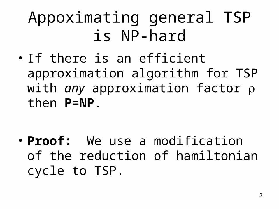
Appoximating general TSP is NP-hard

• If there is an efficient approximation algorithm for TSP with any approximation factor then P=NP.

• Proof: We use a modification of the reduction of hamiltonian cycle to TSP.

3

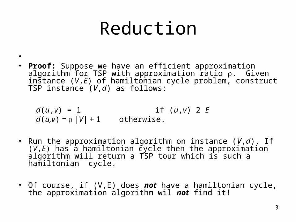
Reduction• • Proof: Suppose we have an efficient approximation algorithm for

TSP with approximation ratio . Given instance (V,E) of hamiltonian cycle problem, construct TSP instance (V,d) as follows:

d(u,v) = 1 if (u,v) 2 E d(u,v) = |V| + 1 otherwise.

• Run the approximation algorithm on instance (V,d). If (V,E) has a hamiltonian cycle then the approximation algorithm will return a TSP tour which is such a hamiltonian cycle.

• Of course, if (V,E) does not have a hamiltonian cycle, the approximation algorithm wil not find it!

4

5

General design/analysis trick

• Our approximation algorithm often works by constructing some relaxation providing a lower bound and turning the relaxed solution into a feasible solution without increasing the cost too much.

• The LP relaxation of the ILP formulation of the problem is a natural choice. We may then round the optimal LP solution.

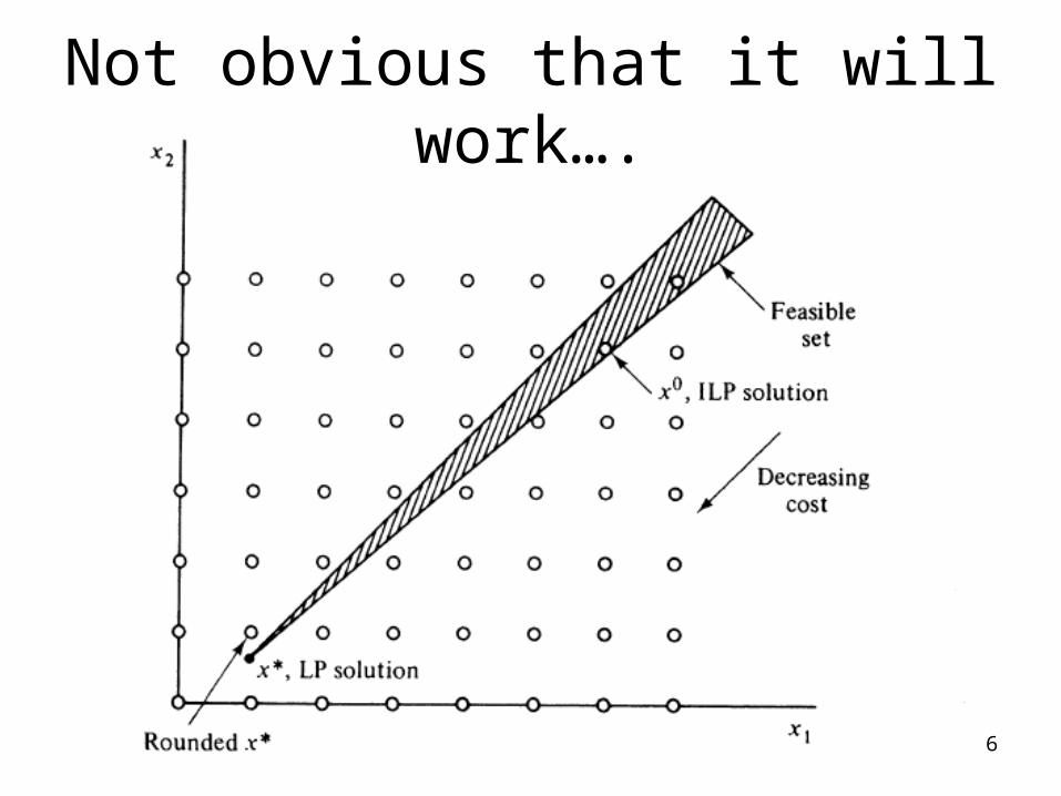
6

Not obvious that it will work….

7

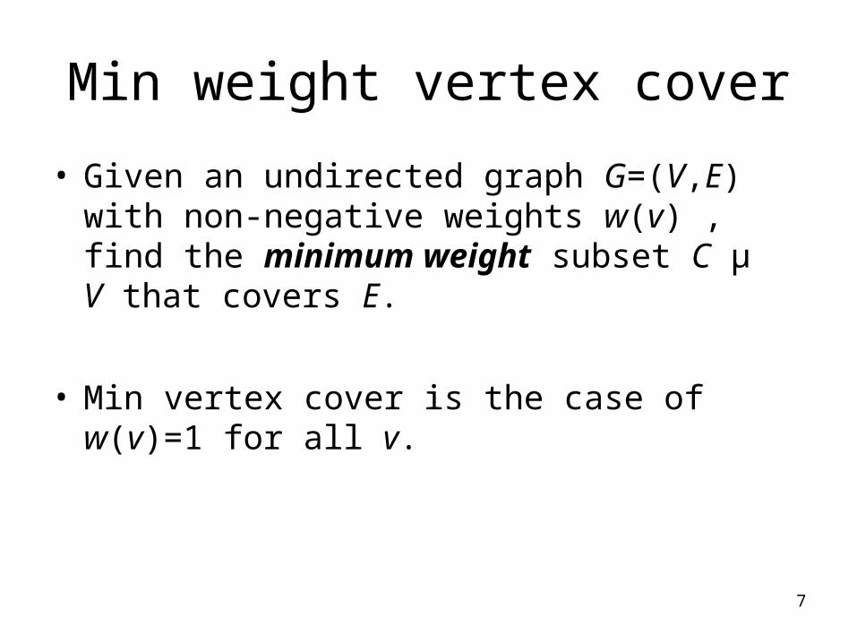
Min weight vertex cover

• Given an undirected graph G=(V,E) with non-negative weights w(v) , find the minimum weight subset C µ V that covers E.

• Min vertex cover is the case of w(v)=1 for all v.

8

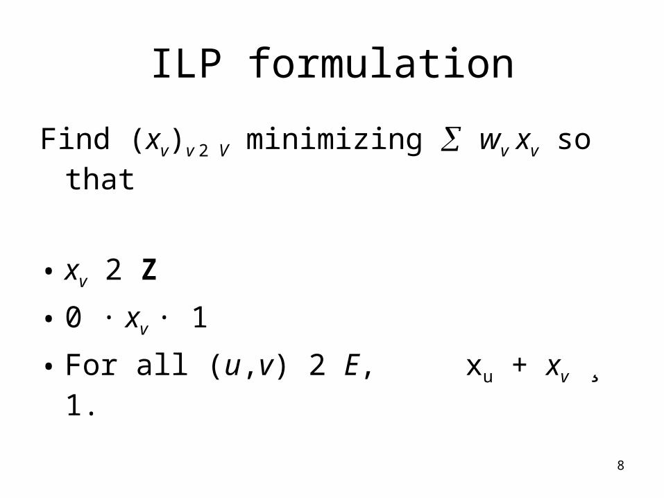
ILP formulation

Find (xv)v 2 V minimizing wv xv so that

• xv 2 Z

• 0 · xv · 1

• For all (u,v) 2 E, xu + xv ¸ 1.

9

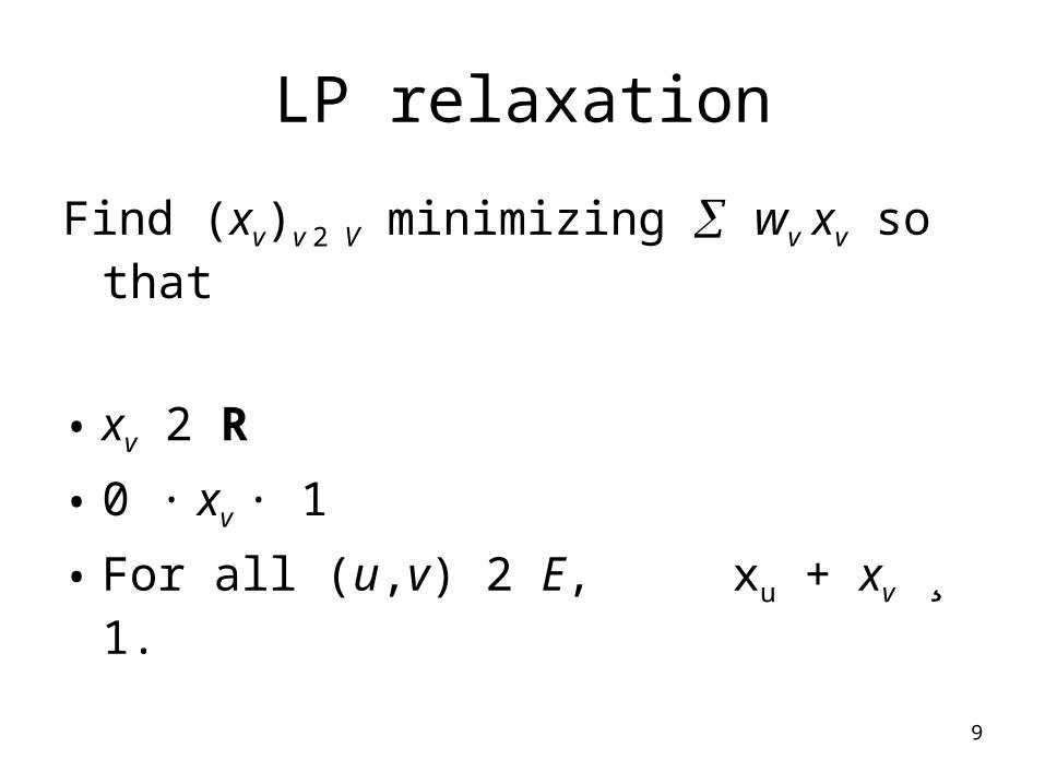
LP relaxation

Find (xv)v 2 V minimizing wv xv so that

• xv 2 R

• 0 · xv · 1

• For all (u,v) 2 E, xu + xv ¸ 1.

10

Relaxation and Rounding

• Solve LP relaxation.

• Round the optimal solution x* to an integer solution x: xv = 1 iff x*v ¸ ½.

• The rounded solution is a cover: If (u,v) 2 E, then x*u + x*v ¸ 1 and hence at least one of xu and xv is set to 1.

11

Quality of solution found

• Let z* = wv xv* be cost of optimal LP solution.

• wv xv · 2 wv xv*, as we only round up if xv* is bigger than ½.

• Since z* · cost of optimal ILP solution, our algorithm has approximation ratio 2.

12

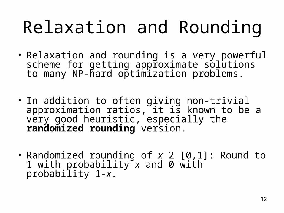
Relaxation and Rounding

• Relaxation and rounding is a very powerful scheme for getting approximate solutions to many NP-hard optimization problems.

• In addition to often giving non-trivial approximation ratios, it is known to be a very good heuristic, especially the randomized rounding version.

• Randomized rounding of x 2 [0,1]: Round to 1 with probability x and 0 with probability 1-x.

13

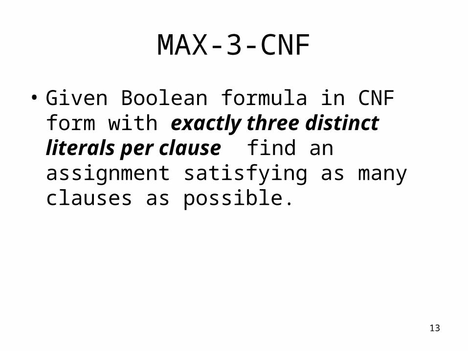
MAX-3-CNF

• Given Boolean formula in CNF form with exactly three distinct literals per clause find an assignment satisfying as many clauses as possible.

14

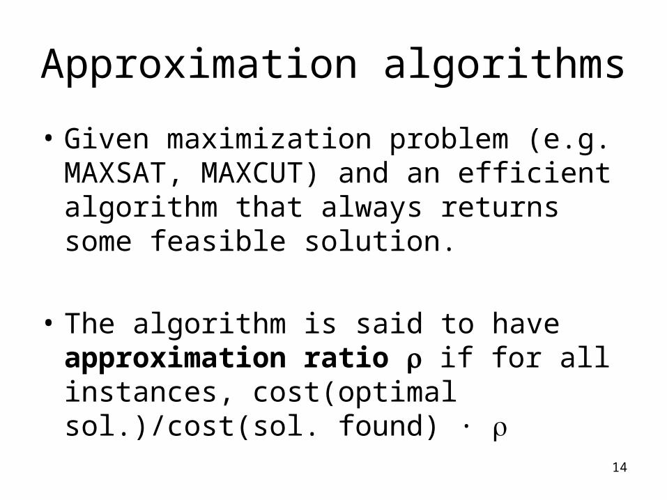
Approximation algorithms

• Given maximization problem (e.g. MAXSAT, MAXCUT) and an efficient algorithm that always returns some feasible solution.

• The algorithm is said to have approximation ratio if for all instances, cost(optimal sol.)/cost(sol. found) ·

15

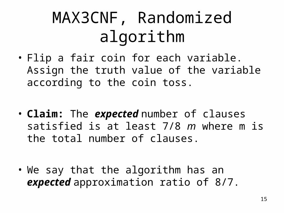
MAX3CNF, Randomized algorithm

• Flip a fair coin for each variable. Assign the truth value of the variable according to the coin toss.

• Claim: The expected number of clauses satisfied is at least 7/8 m where m is the total number of clauses.

• We say that the algorithm has an expected approximation ratio of 8/7.

16

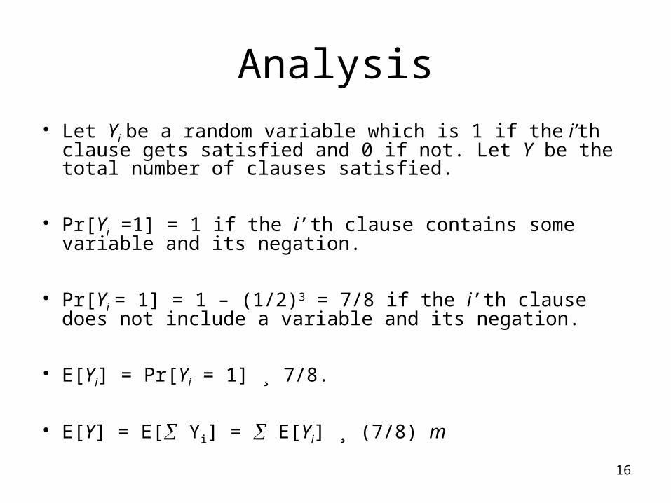
Analysis

• Let Yi be a random variable which is 1 if the i’th clause gets satisfied and 0 if not. Let Y be the total number of clauses satisfied.

• Pr[Yi =1] = 1 if the i’th clause contains some variable and its negation.

• Pr[Yi = 1] = 1 – (1/2)3 = 7/8 if the i’th clause does not include a variable and its negation.

• E[Yi] = Pr[Yi = 1] ¸ 7/8.

• E[Y] = E[ Yi] = E[Yi] ¸ (7/8) m

17

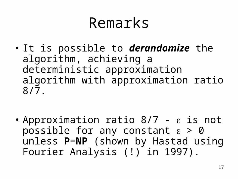
Remarks

• It is possible to derandomize the algorithm, achieving a deterministic approximation algorithm with approximation ratio 8/7.

• Approximation ratio 8/7 - is not possible for any constant > 0 unless P=NP (shown by Hastad using Fourier Analysis (!) in 1997).

18

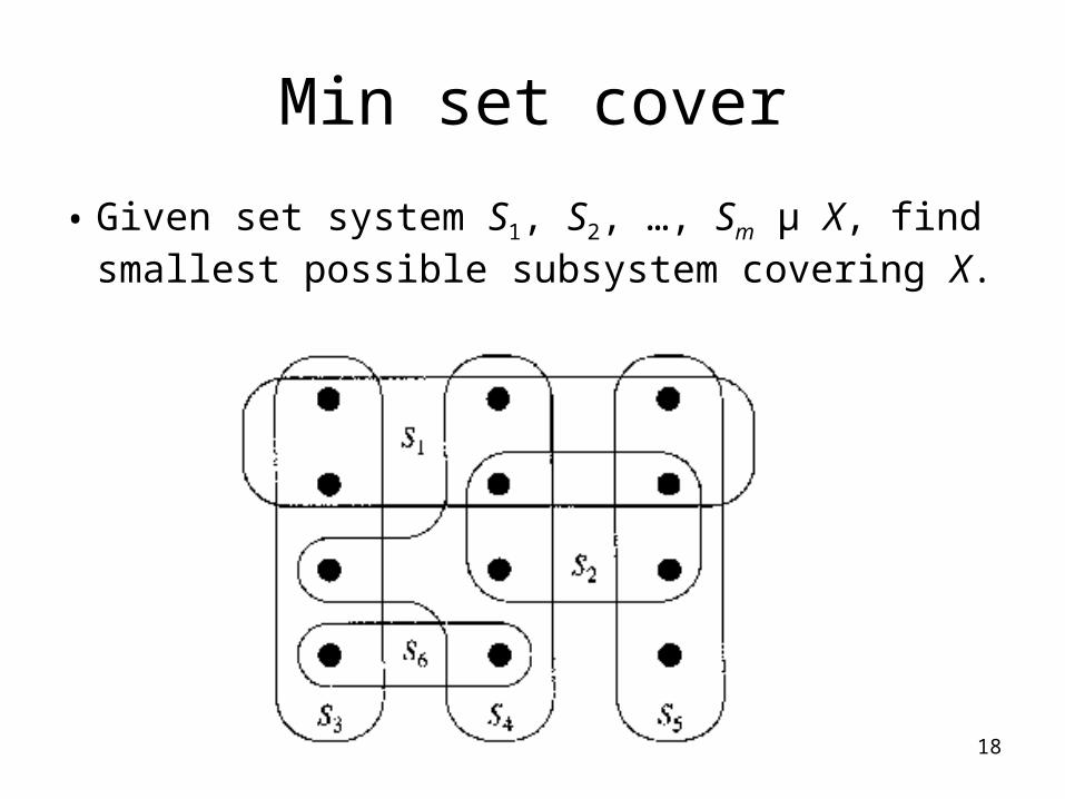
Min set cover

• Given set system S1, S2, …, Sm µ X, find smallest possible subsystem covering X.

19

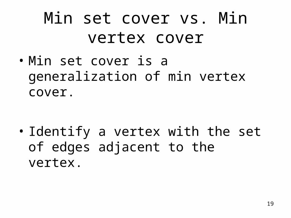
Min set cover vs. Min vertex cover

• Min set cover is a generalization of min vertex cover.

• Identify a vertex with the set of edges adjacent to the vertex.

20

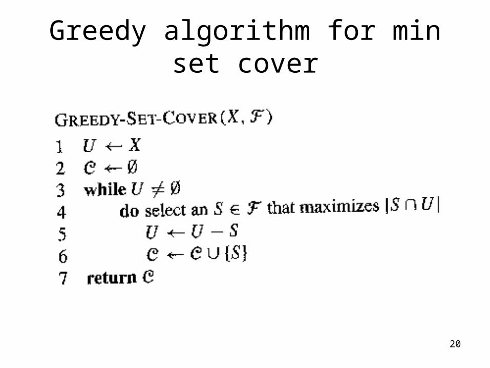
Greedy algorithm for min set cover

21

Approximation Ratio

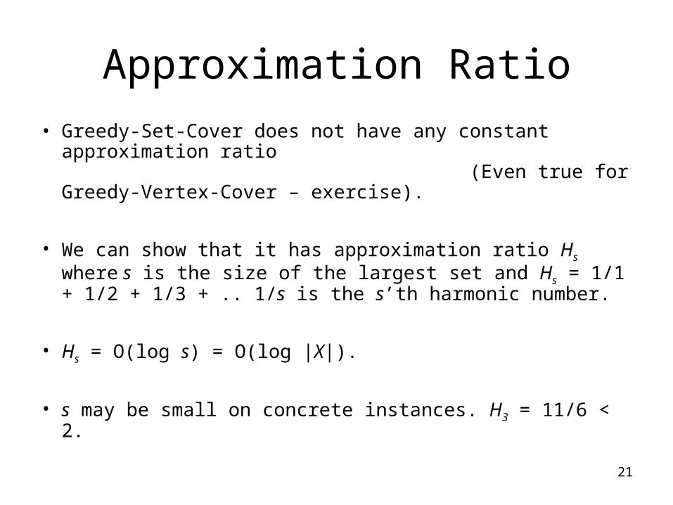
• Greedy-Set-Cover does not have any constant approximation ratio (Even true for Greedy-Vertex-Cover – exercise).

• We can show that it has approximation ratio Hs where s is the size of the largest set and Hs = 1/1 + 1/2 + 1/3 + .. 1/s is the s’th harmonic number.

• Hs = O(log s) = O(log |X|).

• s may be small on concrete instances. H3 = 11/6 < 2.

22

Analysis I

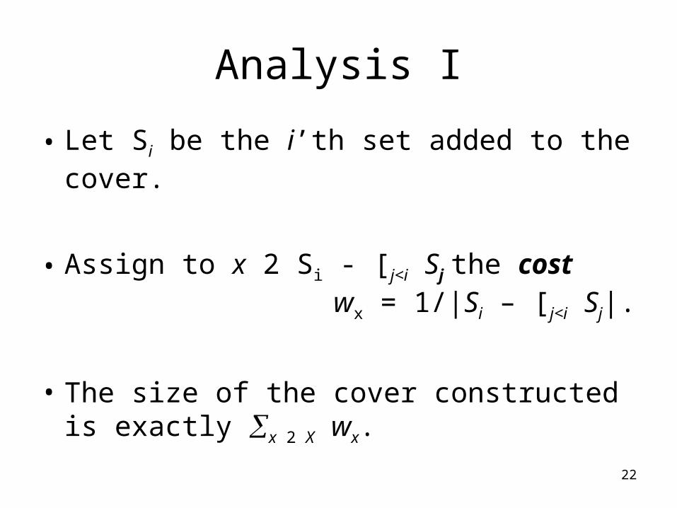
• Let Si be the i’th set added to the cover.

• Assign to x 2 Si - [j<i Sj the cost wx = 1/|Si – [j<i Sj|.

• The size of the cover constructed is exactly x 2 X wx.

23

Analysis II

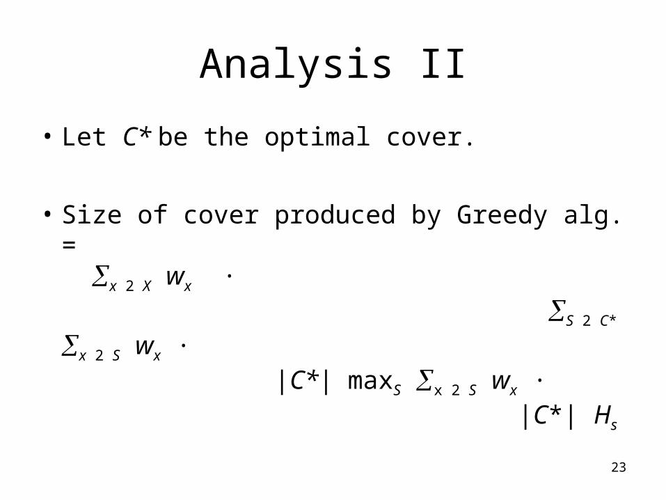
• Let C* be the optimal cover.

• Size of cover produced by Greedy alg. = x 2 X wx · S 2 C* x 2 S wx · |C*| maxS x 2 S wx · |C*| Hs

24

It is unlikely that there are efficient approximation algorithms with a very good approximation ratio for

MAXSAT, MIN NODE COVER, MAX INDEPENDENT SET, MAX CLIQUE, MIN SET COVER, TSP, ….

But we have to solve these problems anyway – what do we do?

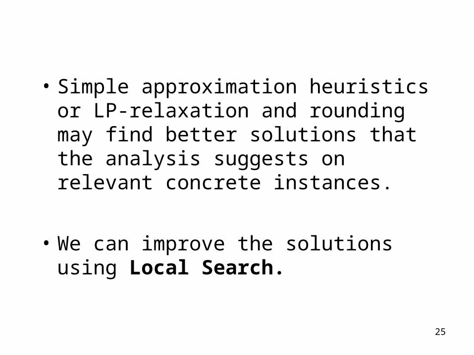
25

• Simple approximation heuristics or LP-

relaxation and rounding may find better solutions that the analysis suggests on relevant concrete instances.

• We can improve the solutions using Local Search.

26

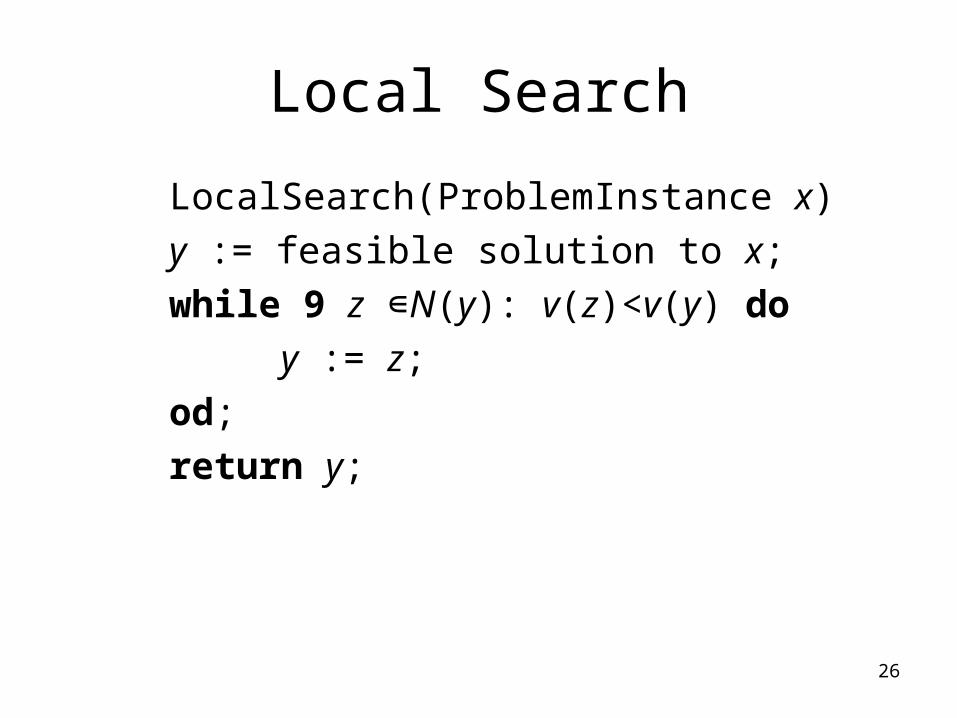
Local Search

LocalSearch(ProblemInstance x)

y := feasible solution to x;

while 9 z ∊N(y): v(z)<v(y) do

y := z;

od;

return y;

27

To do list

• How do we find the first feasible solution?

• Neighborhood design?

• Which neighbor to choose?

• Partial correctness?

• Termination?

• Complexity?

Never Mind!

Stop when tired! (but optimize the time of each iteration).

28

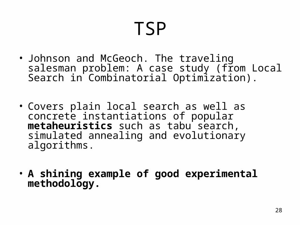
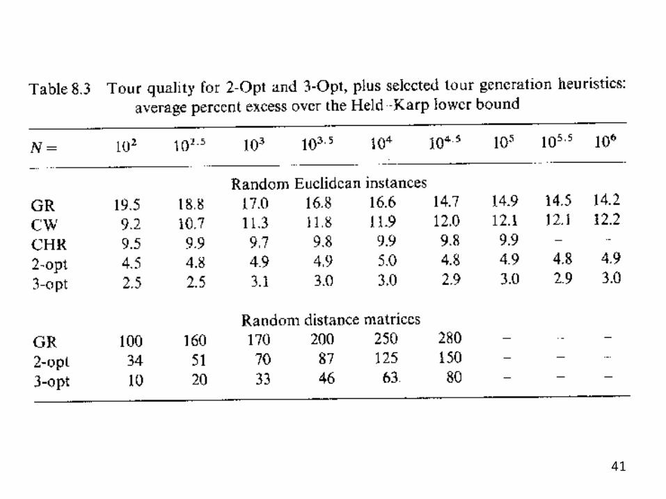
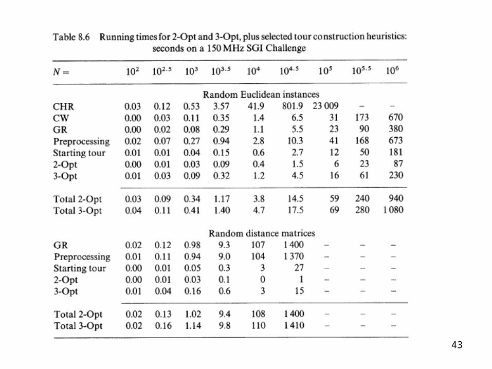
TSP

• Johnson and McGeoch. The traveling salesman problem: A case study (from Local Search in Combinatorial Optimization).

• Covers plain local search as well as concrete instantiations of popular metaheuristics such as tabu search, simulated annealing and evolutionary algorithms.

• A shining example of good experimental methodology.

29

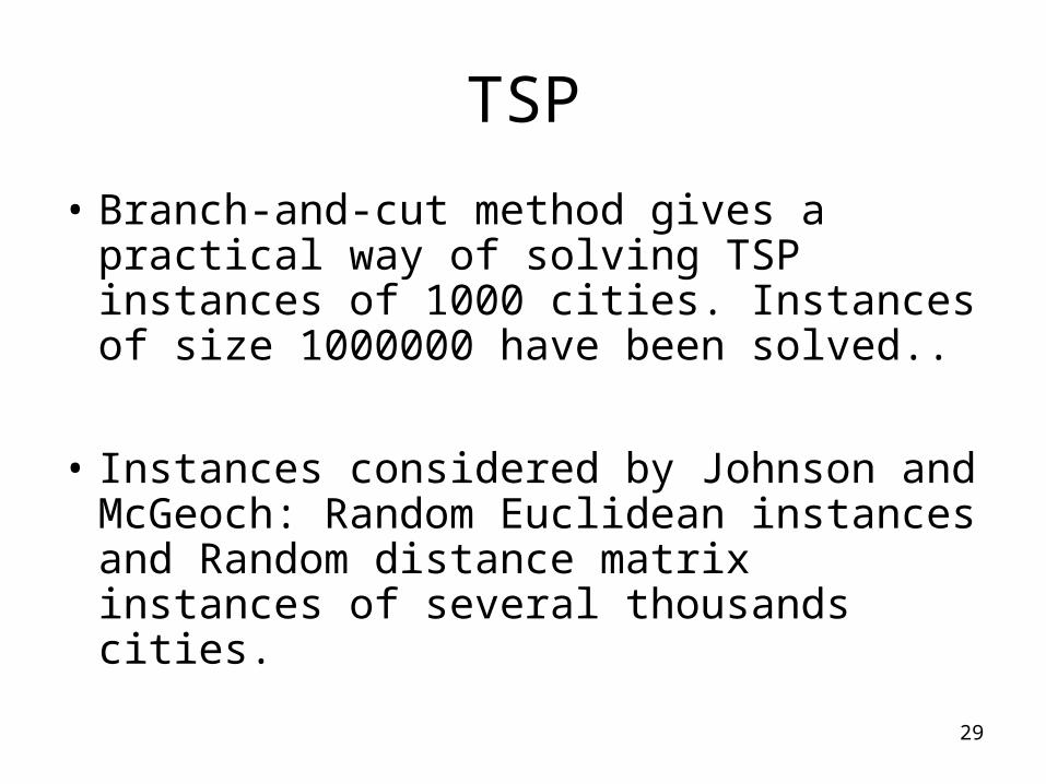
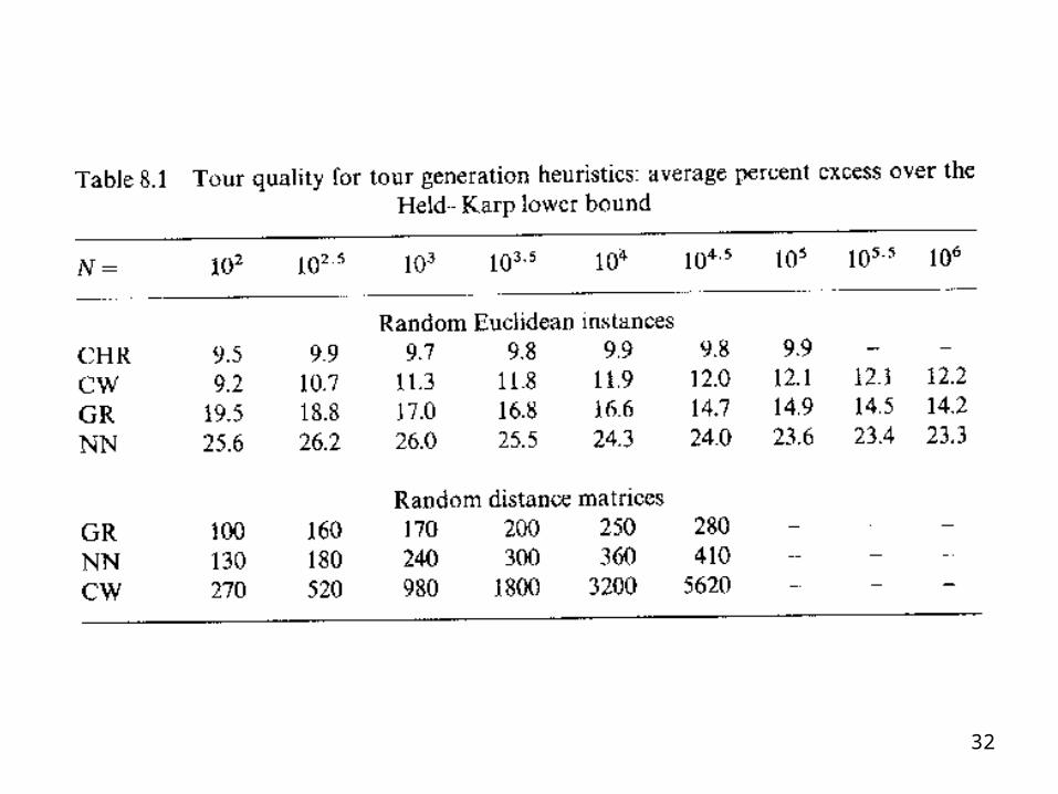
TSP

• Branch-and-cut method gives a practical way of solving TSP instances of 1000 cities. Instances of size 1000000 have been solved..

• Instances considered by Johnson and McGeoch: Random Euclidean instances and Random distance matrix instances of several thousands cities.

30

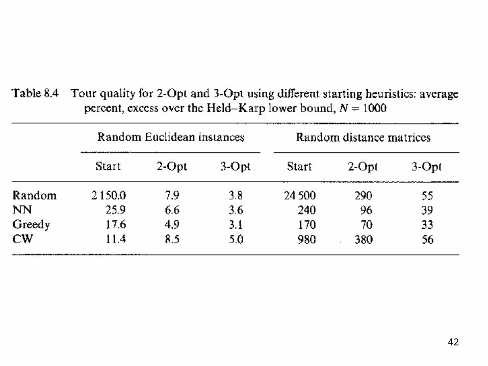
Local search design tasks

• Finding an initial solution

• Neighborhood structure

31

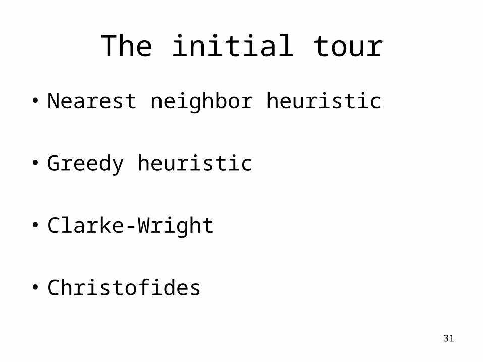
The initial tour

• Nearest neighbor heuristic

• Greedy heuristic

• Clarke-Wright

• Christofides

32

33

Neighborhood design

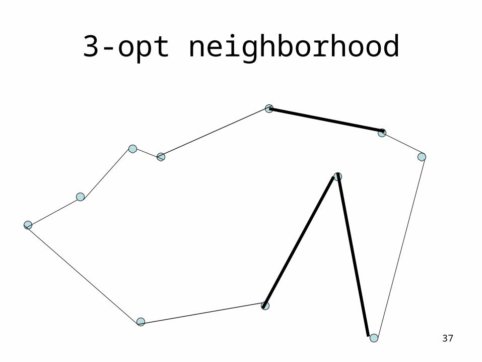
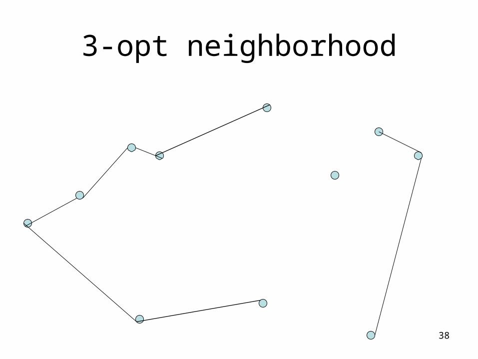
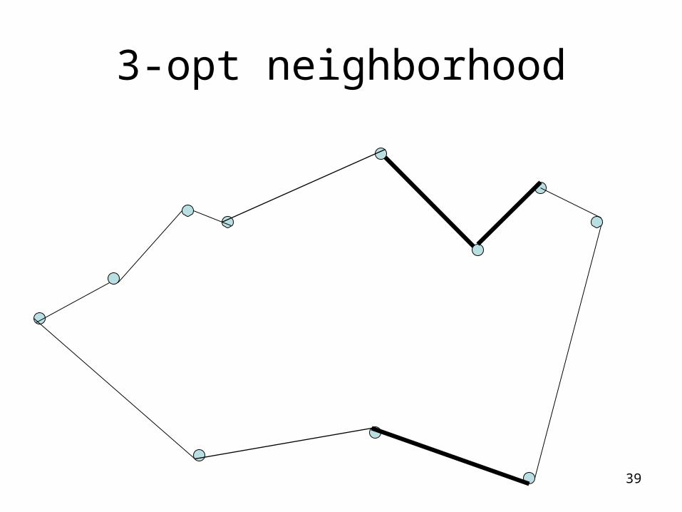
Natural neighborhood structures:

2-opt, 3-opt, 4-opt,…

34

2-opt neighborhood

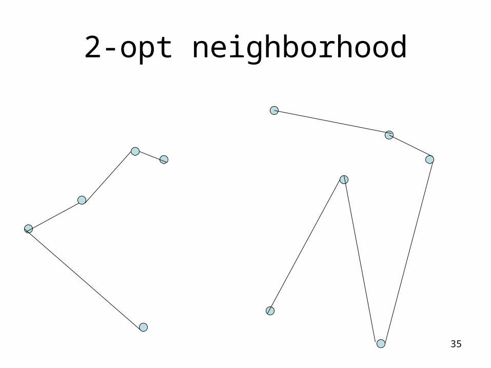
35

2-opt neighborhood

36

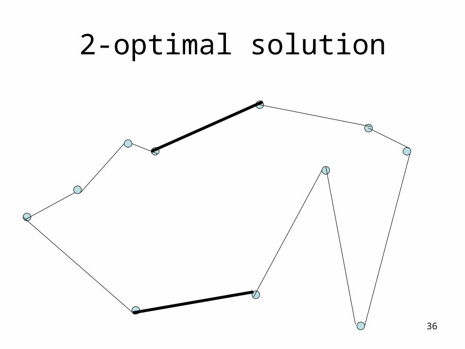
2-optimal solution

37

3-opt neighborhood

38

3-opt neighborhood

39

3-opt neighborhood

40

Neighborhood Properties

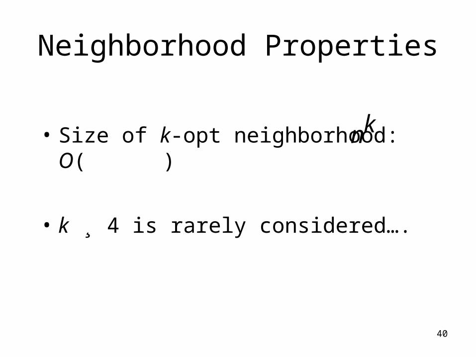
• Size of k-opt neighborhood: O( )

• k ¸ 4 is rarely considered….

kn

41

42

43

44

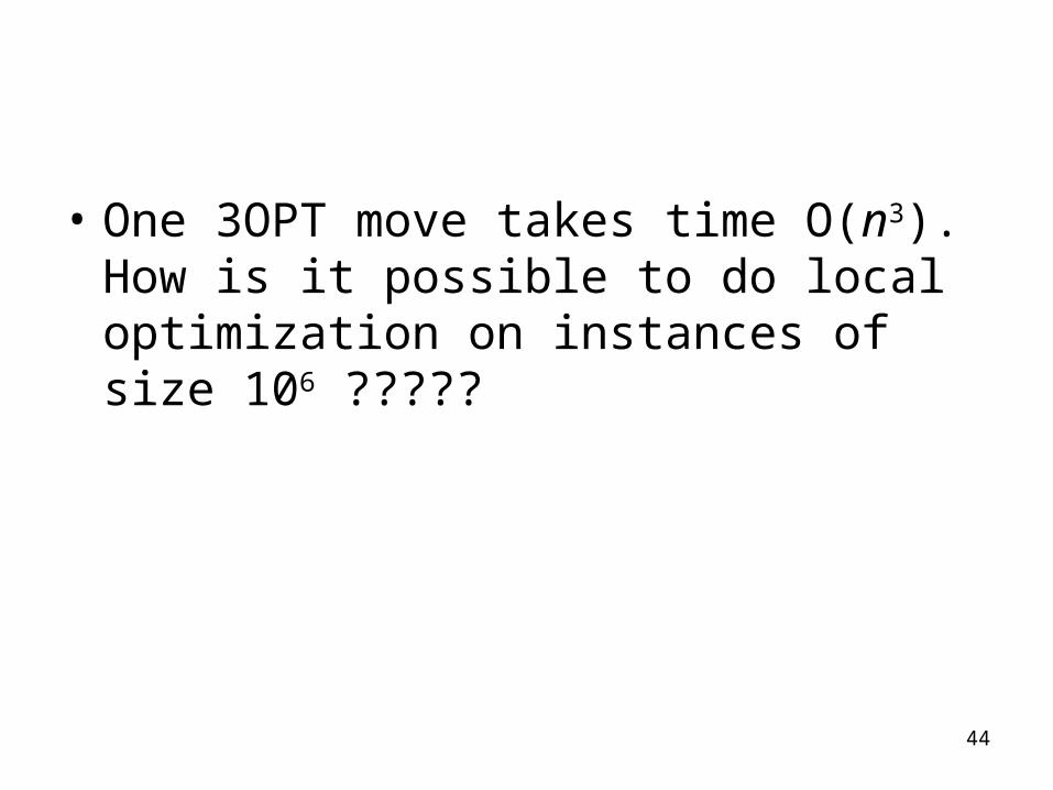
• One 3OPT move takes time O(n3). How is it possible to do local optimization on instances of size 106 ?????

45

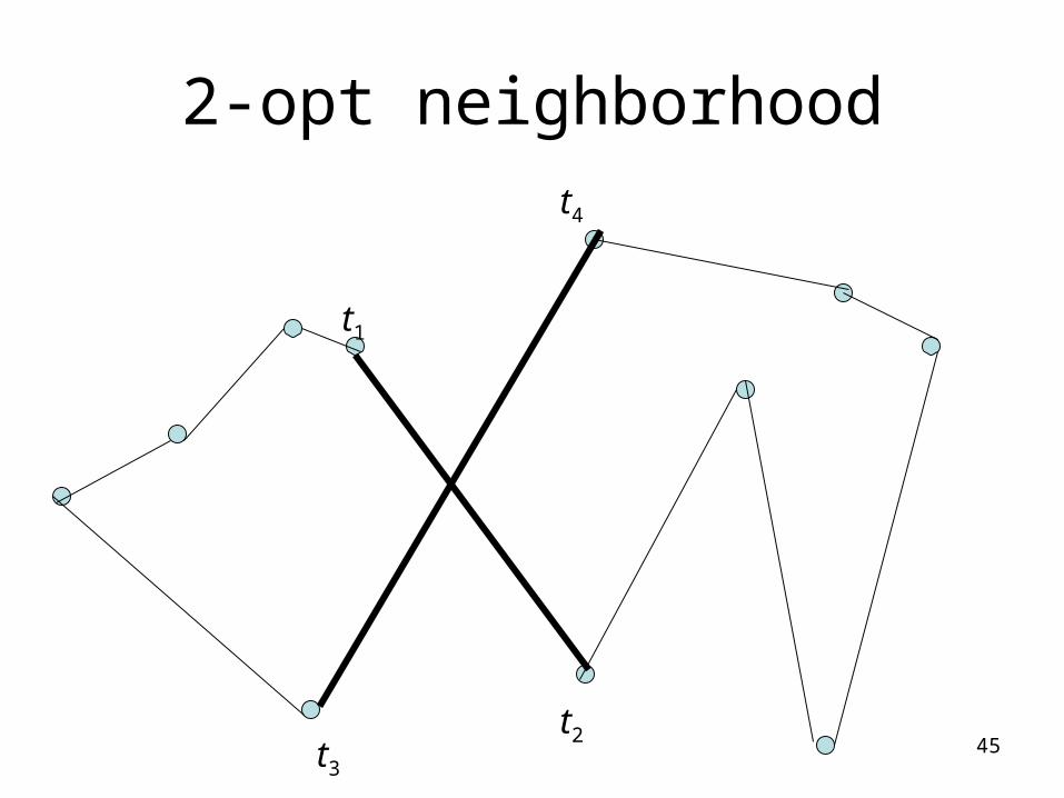
2-opt neighborhood

t1

t4

t3

t2

46

A 2-opt move

• If d(t1, t2) · d(t2, t3) and d(t3,t4) · d(t4,t1), the move is not improving.

• Thus we can restrict searches for tuples where either d(t1, t2) > d(t2, t3) or d(t3, t4) > d(t4, t1).

• WLOG, d(t1,t2) > d(t2, t3).

47

Neighbor lists

• For each city, keep a static list of cities in order of increasing distance.

• When looking for a 2-opt move, for each candidate for t1 with t2 being the next city, look in the neighbor list for t2 for t3 candidate. Stop when distance becomes too big.

• For random Euclidean instance, expected time to for finding 2-opt move is linear.

48

Problem

• Neighbor lists becomes very big.

• It is very rare that one looks at an item at position > 20.

49

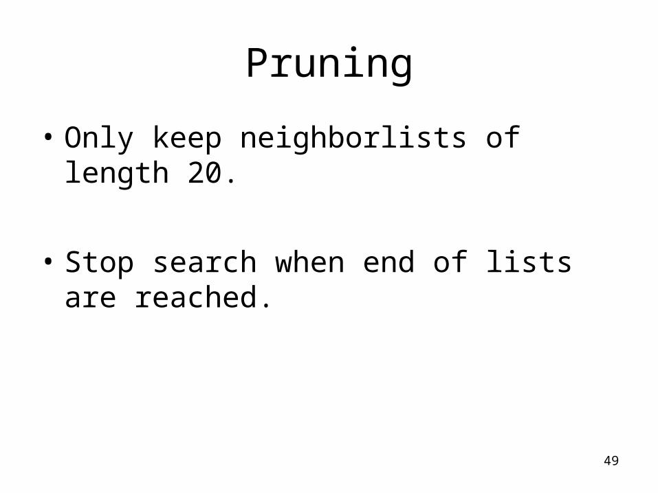
Pruning

• Only keep neighborlists of length 20.

• Stop search when end of lists are reached.

50

• Still not fast enough……

51

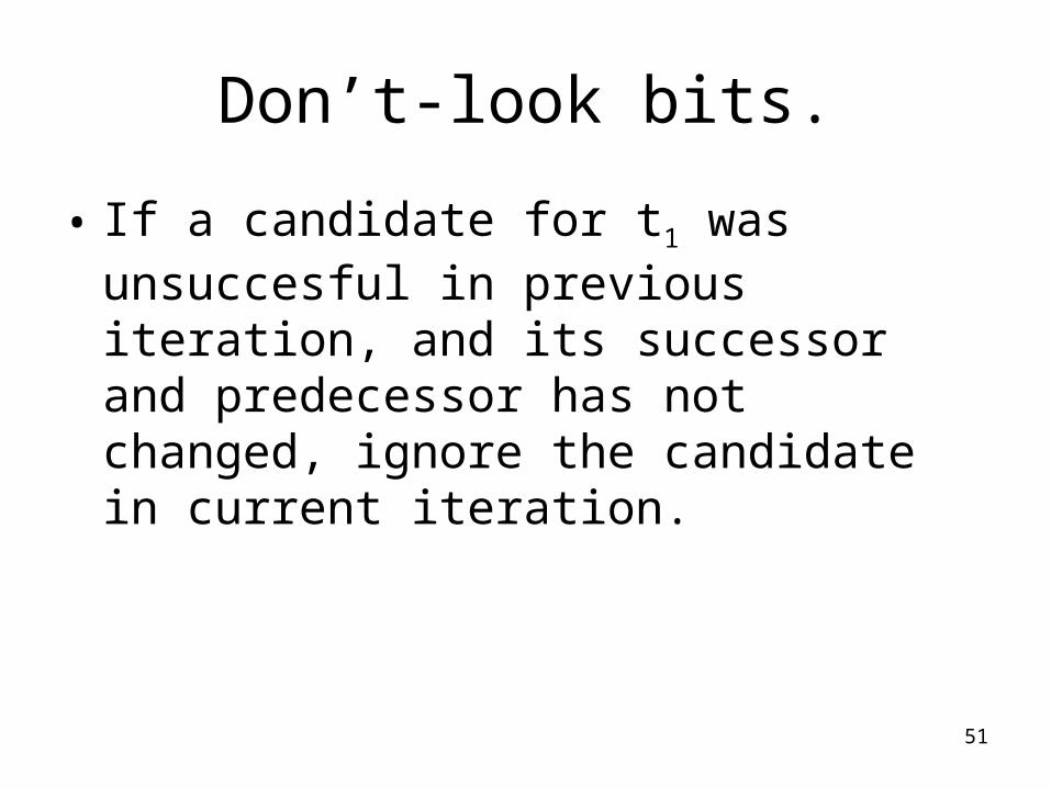
Don’t-look bits.

• If a candidate for t1 was unsuccesful in previous iteration, and its successor and predecessor has not changed, ignore the candidate in current iteration.

52

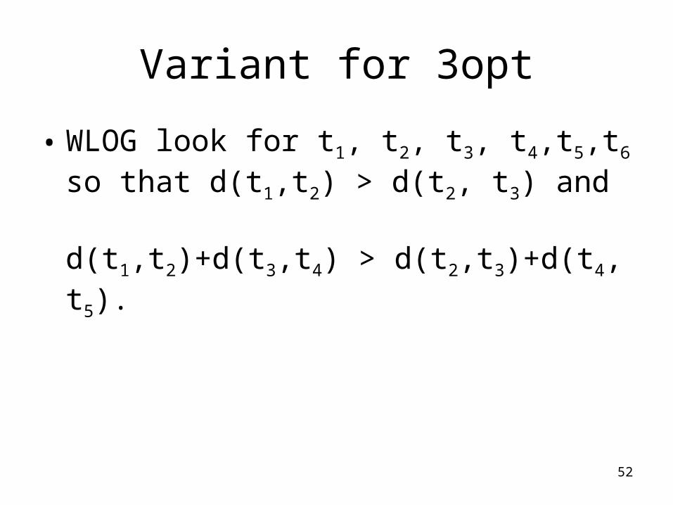
Variant for 3opt

• WLOG look for t1, t2, t3, t4,t5,t6 so that d(t1,t2) > d(t2, t3) and d(t1,t2)+d(t3,t4) > d(t2,t3)+d(t4, t5).

53

On Thursday

….we’ll escape local optima using Taboo search and Lin-Kernighan.