Perspectives 50

STRATEGIES FOR SAMPLE ATTRITION ANALYSES IN THE NA-TIONAL SURVEY OF BLACK AMERICANS

Marc A. Musick, Assistant Professor, Department of Sociology, Population ResearchCenter, The University of Texas at Austin

Anna M. Campbell, Graduate Research Assistant, Department of Sociology, Popula-tion Research Center, The University of Texas at Austin

Christopher G. Ellison, Associate Professor, Department of Sociology, PopulationResearch Center, The University of Texas at Austin

Introduction

Since its inception in 1979-80, the National Survey of Black Americans (NSBA) hasserved as an extensive storehouse of information on African Americans for research-ers around the U.S. Studies using the NSBA have focused on numerous topics in avariety of fields, including religion (e.g., Ellison and Sherkat 1990; Sherkat and Ellison1991), mental and physical health (e.g., Jackson, et al. 1996; Johnson and Broman1987; Neighbors, et al. 1983), family (e.g., Taylor and Chatters 1991), social support(Lewis 1989; Taylor and Chatters 1986), and health and social services utilization(Neighbors 1985; Neighbors, Musick and Williams 1998; Taylor, Neighbors, andBroman 1989). Clearly, the data set has provided insights into the lives of AfricanAmericans that would have been difficult to gain through other mechanisms.

Following the initial wave of data collection in 1979-80, NSBA staff collected dataover 3 subsequent waves in 1987-88, 1988-89, and 1992. Researchers have and con-tinue to use these data to examine the multiple topics, including those listed above.However, the NSBA faces a major limitation that is encountered by all longitudinaldata sets but is difficult to remedy: sample attrition. By the fourth wave in 1992,approximately 1,456 respondents, or 69% of the original sample size, had departedthe sample. Most of the sample attrition (n = 1,301 or 62%) was non-mortality attri-tion. That is, sample respondents left the survey due to refusal, an inability to partici-pate, or because the survey staff were unable to reach them.

Sample attrition over time is a problem due to the patterned nature of the attrition.For example, a variety of research (e.g., Pappas, et al. 1993, Rogers, et al. 2000,Sorlie, et al. 1995) has shown that mortality over time is non-random; that is, it ispatterned by certain factors, such as age, socioeconomic status, and health. Researchhas indicated that non-mortality attrition is also non-random. Indeed, Wolford andTorres (2001) documented this fact for the NSBA sample. When sample attrition is

Perspectives 51

non-random and cases from reduced latter waves are used, it is possible that anyestimates arrived through regression analyses will be problematic (Breen 1996;Heckman 1979). Consequently, it has been argued that adjustments must be made tothe analyses to account for the possible biases that might result. Although, morerecently some researchers, notably Stolzenberg and Relles (1997) have argued thattechniques used to adjust for attrition bias can be overused and thus produce errone-ous results. Nevertheless, it is reasonable to expect that techniques designed to over-come the attrition problem should be used whenever analyzing data from the latterthree waves of the NSBA.

The purpose of this paper is to explore the sample selection issue within the NSBA.Drawing on the findings of Wolford and Torres (2001), we construct models to pre-dict selection within the NSBA. However, we go beyond the work of Wolford andTorres by incorporating additional variables that are significant predictors of attri-tion. Once we establish the attrition models, we provide a substantive example usingdata from the fourth wave of the NSBA. In this example, we show estimates that areunadjusted for attrition compared to those that are adjusted using two different meth-ods. This example focuses on distress, a topic which has been previously examinedin the fourth wave of the NSBA (e.g., Ellison, et al. 1997).

Readers should note that our goal here is to provide a guide to constructing sampleattrition models with the NSBA data. Keeping that in mind, we will attempt to pro-vide an explicit rationale for the models and for the variables we include in the mod-els. Moreover, we provide detailed explanations of the variables used in our analysesto facilitate replication and extension in future NSBA studies. Our goal is to showthat attrition is a matter of serious concern in the NSBA, but one that can be mini-mized with the proper procedures.

Predicting Attrition

If we consider that attrition falls into one of two categories, mortality and non-mortal-ity, then the task of searching for predictors of attrition becomes somewhat easier. Anumber of studies oriented towards understanding the mortality process have docu-mented the factors that often contribute to increased mortality. Here we review sev-eral sets of these factors, many of which would overlap with the non-mortality type.

Mortality-based Attrition

Sociodemographics. Generally speaking, research shows that a number ofsociodemographic factors are associated with mortality. For instance, men, olderadults, those living in urban areas, and unmarried adults all carry greater risk of mor-tality (Lantz, et al. 1998; Rogers, Hummer and Nam 2000; Smith, et al. 1995). Other

Perspectives 52

research (e.g., Kaplan 1996) has suggested that household characteristics, such ascrowding, might have effects on individual mortality rates as well. Consequently,studies of attrition should attempt to account for these sorts of factors.

Socioeconomic Status. One set of factors receiving a great deal of attention in themortality process is socioeconomic status (SES). In essence, research using popula-tions both in the U.S. and abroad shows that adults with lower SES tend to have worsehealth and higher mortality rates (e.g., Lantz, et al. 1998; Rogers, Hummer and Nam2000). In these studies, SES is measured in a variety of ways, including educationlevel, family or personal income, occupation, and wealth. Given the strong associa-tion between SES and mortality noted in previous studies, it is likely that these factorswill emerge as significant predictors of attrition within the NSBA.

Employment. Related to the research on socioeconomic status, studies of the effectsof unemployment and work factors have shown the importance of these factors forlongevity. Findings indicate that adults who are unemployed or who face hazardousor stressful work conditions are at greater risk for mortality compared to those whowork and have jobs that are characterized by safe and stable work environments (Smith,et al. 1998). Without firm data on the nature of the work environment, it can bedifficult to ascertain the nature of the work involved. However, through measuressuch as job prestige and similar factors, we can arrive at approximations of the workexperience.

Community Involvement and Social Integration. A number of studies have focusedon the role that community involvement and social integration play in the mortalityprocess. For example, Moen and her colleagues (1989) showed that women whowere active members of an organization had lower mortality rates than their uninvolvedcounterparts over a 30-year follow-up period. In their work in Tecumseh, Michigan,House and his colleagues (1982) showed similar findings for participation in organi-zational meetings. Another set of research focuses specifically on involvement inreligious institutions and how those affect the mortality process. In general, thesestudies show that respondents who are more involved in the church tend to live longerthan those who are less involved (e.g., Hummer, et al. 1999; Strawbridge, et al. 1997).

Health. Perhaps one of the strongest predictors of mortality shown through numer-ous studies is respondent health status. Most studies of mortality show that poorhealth, measured along multiple dimensions, is predictive of greater mortality risk.More specifically, authors have noted strong associations with self-rated health(Greiner, et al. 1996; Idler and Benyamini 1997; Idler and Kasl 1991; Wolinsky andJohnson 1992), functional health (Rogers, Hummer and Nam 2000), and the pres-ence of chronic health conditions (Musick, Herzog and House 1999). Any studypurporting to predict sample attrition over time, especially in terms of mortality, should

Perspectives 53

adjust for these factors.

Non-mortality Attrition

Ordinarily, non-mortality forms of attrition break down into three main forms. First,respondents may have departed the sample because they simply refused to cooperatewith the additional waves. Second, data staff might be unable to locate, and thereforeinterview, respondents. Third, respondents might be incapacitated, either throughhealth problems, institutionalization, incarceration, or enlistment in military servicerendering them difficult if not impossible to interview. Given these three forms ofnon-mortality attrition, we should look for sets of factors that would apply to one ormore.

Of the factors outlined above for mortality, several non-mortality predictors are pos-sible. First, good health in the first wave might be indicative of people who would notbe incapacitated or institutionalized (e.g., in a nursing home) during later waves.Consequently, we would expect that healthy first wave respondents would more fre-quently appear in latter waves.

Second, high levels of socioeconomic status should lead people to be more coopera-tive with the survey. Indeed, we know that higher SES is associated with other formsof community participation, such as volunteering and participating in other formalorganizations (Wilson and Musick 1997); it is likely the same processes underlyingthe linkage between SES and these activities would hold true for survey research. Inaddition, higher levels of SES might be indicative of stability. Given that much of thesample attrition in the NSBA is due to the inability of the survey staff to relocaterespondents, those with greater residential stability in the first wave will be morelikely to be relocated during subsequent waves. In this regard, whether the respon-dents own their homes is a potentially strong predictor given that homeowners aremore tied to their residences and thus are less likely to move. In fact, Wolford andTorres (2001) found that one of the strongest predictors of attrition in the NSBA washome ownership. Another indicator of SES, education, might have substantial im-pacts on attrition in the following way: more educated respondents might place ahigher value on the survey and its goals leading to a greater willingness to participate.

Third, active involvement in the community should predict greater retention. It shouldbe the case that respondents who are engaged in their community will feel more a partof the community and therefore will have more residential stability and be easier tolocate. Further, even if involved respondents had moved, it is possible that friendsand neighbors in the community will know enough about respondents’ new residencesto help relocation efforts. Active involvement in community life might also be in-dicative of an underlying proclivity to participate in voluntary activities, such as re-

Perspectives 54

search studies. In this regard, work by Ellison (1992) indicates that more religiousAfrican Americans tend to be more cooperative in interview settings. Consequently,we should see fewer refusals among active community members, and especially reli-gious respondents, than among those who are not as active.

Other factors, such as employment status and residence might also play a part inpredicting non-mortality attrition. Respondents with steady jobs will be those lesslikely to relocate residences. Further, given the tight-knit nature of less urban com-munities (Beggs, Haines and Hurlbert 1996), people living in less urban areas may belocated relatively easily through friends and family even if they have changed resi-dences. In sum, there are a number of ways in which the factors listed above couldaffect sample attrition both in terms of mortality and non-mortality mechanisms.

The Utility of Interviewer Observations

Researchers can use variables in many of the areas listed above in their studies tocontrol the effects of sample attrition. A problem arises, however, when the substan-tive outcome of the study is predicted by many of the same variables as the sampleattrition. For example, given the processes outlined above, a researcher wanting tostudy changes in health across the waves would probably use many of the variableslisted above to predict changes in health status. If those same variables are used in theselection models, a problem could arise. More specifically, the variables used in theselection model must be somewhat different than those in the substantive model,otherwise the selection model will be unable to effectively adjust for the selectionprocess. Indeed, as Breen (1996) has noted, if all of the variables in the selectionmodel overlap with the variables in the substantive model, the predictive power of theselection portion rests only in the non-linearity in the probit model used to computethe selection adjustments. Consequently, a major goal for constructing proper sampleselection models is to use as many non-overlapping factors as possible in the selec-tion and substantive models.

One source of non-overlapping factors that often go unused in surveys is the inter-viewer observations. Interviewers are commonly asked to assess the respondents’demeanor during the interview, the state of their home and neighborhood, their health,and their overall apparent quality of life. Researchers can tap these measures aspossible predictors of selection as many of the variables fall into the same categoriesas those listed above. In general, few researchers have used these measures in theNSBA. Yet, in the few cases where these measures have been used, they have yieldedvaluable information (e.g., Ellison 1993; Hughes and Hertel 1990; Keith and Herring1991). On the topic of attrition, Wolford and Torres (2001) used interviewers’ obser-vations of respondents’ income in the first wave of the NSBA. Such a measure couldbe used as an independent appraisal of the respondents’ overall SES and can be used

Perspectives 55

in conjunction with the SES measures provided by respondents themselves. Othermeasures in the NSBA ask interviewers to rate how interested respondents seemed inthe interview, whether they were impatient, were having difficulty hearing words, orwere reluctant about signing the re-contact form. In short, variables such as thesepotentially contain great utility for predicting attrition. Moreover, because they areunlikely to be used in predicting most substantive topics, their usage will not overlapwith the variables in the main models.

Data and Methods

Sample

The data used in this analysis are taken from all four waves of the National Survey ofBlack Americans, a probability sample of 2,107 African Americans (Jackson and Gurin1997). The first wave of the study was conducted using face-to-face interviews in1979-80. Follow-up surveys were conducted using phone interviews in 1987-88(N=931), 1988-89 (N=785), and 1992 (N=651).

Attrition Measures

Socioeconomic Status. Socioeconomic status was measured using four variables.The first measure (Home Ownership) is coded one if respondents own their homesand zero otherwise. Education is categorized into four groups: (1) 0 to 11 years, (2)12 years or high school graduate, (3) 13 to 15 years or some college, and (4) 16 yearsor more or college graduate. Personal Income is grouped into eight categories rang-ing from 0 to $15,000 or more. Interviewers’ estimation of respondent income (LowIncome – IW) was coded one if interviewers felt the respondent’s income fell below$10,000 per year and zero otherwise. The final measure (No Problems Paying Bills)asks how much respondents worry that their total family income will not be enoughto meet expenses and bills. The response categories range from (1) a great deal to (4)not at all.

Sociodemographics. All models were adjusted for the effects of sociodemographiccharacteristics including gender (Female: 0 = male, 1 = female), living in a threegeneration family (Three Generation Family: 0 = no, 1 = yes), number of personsliving in the household (Number in HH) ranging from 0 to 13, and living in a self-representing urban area (Urban Residence: 0 = no, 1 = yes).

Employment. The first measure of employment (Employment Search Status) is codedone if the respondent was laid off or not working at all and zero if otherwise. Thesecond measure (Employed only Part of 1978) is coded one if the respondent did notwork for some weeks in 1978 and zero if otherwise. The most important factor in a

Perspectives 56

job (Most Important Job Factor) is coded one if the respondent reported friendlypeople to work with and zero if otherwise. Frequency of absence from work (Ab-sence from Work) is coded one if the respondent reported missing work very oftenand zero otherwise. Finally, wage type (Paid a Salary) is coded one if the respondentis paid a salary and zero otherwise.

Community Involvement. Level of community involvement is measured using threevariables. Whether or not the respondent voted in the last presidential election (Votedin Presidential Election) is coded one for yes and zero if otherwise. Frequency ofchurch activity besides attendance at regular services (Church Activity) is coded onefor nearly everyday or more zero otherwise. An additional variable is included tomeasure whether or not the topic of the study affected nonresponse. Whether or notthe respondent would vote for a candidate with the best platform for blacks even if he/she did not belong to the respondent’s party (Supports Black Platform) is assigned avalue of one for yes and zero otherwise.

Interviewer Observations. Several measures were used in order to assess individual’saffective states and attitudes toward the survey (as observed by the interviewer) atbaseline on the likelihood of their participation in subsequent waves. These includewhether or not the respondent ever asked how much longer the interview would take(Asked Interview Length: 0 = no, 1 = yes), ever had difficulty with any of the wordingused in the interview (Difficulty with Words: 0 = no, 1 = yes), was reluctant to signthe recontact sheet (Reluctant to Sign Re-contact: 0 = no, 1 = yes), and if therespondent’s home appeared to be in need of minor (Minor Repairs Needed: 0 = no,1 = yes) or major repairs (Major Repairs Needed: 0 = no, 1 = yes). For the latter twovariables, the reference category was no repairs appeared needed. A three-item indexof physical problems (Physical Problems) was coded one if the respondent had hear-ing problems, vision problems such as blindness or unusually thick lenses, or physi-cal impairments such as missing limbs, artificial limbs, facial scars, etc. and zero if noproblems were reported.

Psychological Distress Example

The variables gender, employment search status, education, and problems payingbills as described above are also included in the distress example. Additional mea-sures included in the distress example are grouped into the following categories: socio-demographics, religion, social integration, and health and well-being.

Psychological Distress. Distress was measured in the fourth wave using an indexcreated by taking the arithmetic mean of ten items: (a) under strain, stress or pressure;(b) in low or very low spirits; (c) been moody or brooded about things; (d) felt down-hearted and blue; (e) feel depressed; (f) felt tense or high-strung; (g) able to relax

Perspectives 57

(reverse-coded); (h) bothered by nervousness or your nerves; (i) felt restless and up-set; and (j) been anxious and worried. For each of the items, respondents were askedhow much they had felt that way over the past month. Responses range from (1) noneof the time to (4) all of the time.

Sociodemographics. All models were adjusted for the effects of certain social anddemographic characteristics including, age (Age: in years), marital status (Married: 0= not married, 1 = currently married), and family income (Family Income: in catego-ries ranging from 0 to $30,000 or more).

Religion. We include three measures of religious attendance and practice. First,Religious Attendance asks respondents how often they usually attend religious ser-vices. The five response categories include (1) less than once a year or never, (2) afew times a year, (3) a few times a month (1 to 3 times), (4) at least once a week (1 to3 times), and (5) nearly everyday (4 or more times a week). The second and thirdvariables indicate how often the respondent prays. The responses range from (1)never to (5) nearly everyday or 4 or more times per week. It should be noted that wecentered the prayer variable (Prayer) and then squared it (Prayer2) to estimate curvi-linear effects.

Social Integration. The first measure of social integration (Confidants) indicates howmany friends, not including relatives, the respondent feels free to talk with about theirproblems. The response categories range from (1) none to (4) many. The secondmeasure (Social Interaction) asks how often the respondent sees, writes, or talks onthe telephone with friends. The response categories range from (1) hardly ever ornever to (6) nearly everyday or 4 or more times per week. Finally, we include a two-item index of family support that asks respondents (a) how often people in their fam-ily help them out, and (b) how much help they are. The response categories rangefrom (1) never to (4) very often, and from (1) only a little help to (4) a great deal ofhelp, respectively.

Health and Well-Being. Health and well-being are measured using three variables. Inorder to measure the degree of personal problems, respondents were asked whetheror not they had ever (a) had a personal problem they could not handle themselves, (b)felt down and depressed, so low they could not get along, (c) had a personal problemwhere they felt so nervous they could not do much of anything, or (d) felt they wereabout at the point of a nervous breakdown. We created a new variable (Mental HealthProblems) with response categories that range from (1) never experienced any ofthese personal problems to (5) felt they were about at the point of a nervous break-down (categories a, b, and c from above were coded 2, 3, and 4, respectively). Self-esteem is a six-item index created using the following items: (a) I am a useful personto have around; (b) I feel that I’m a person of worth; (c) As a person, I do a good job

Perspectives 58

these days; (d) I feel I do not have much to be proud of; (e) I feel that my life is notvery useful; and (f) I feel that I can’t do anything right. For each item, respondentswere asked to indicate whether the statement was (1) never true, (2) not often true, (3)often true, or (4) almost always true of them. The latter three items were reversecoded so that higher scores are indicative of greater self-esteem. Finally, functionalhealth at the first wave (Wave 1 Functional Health) is a sum of the number of thefollowing debilitating conditions that keep the respondent from working or carryingout their daily tasks: arthritis/rheumatism, ulcers, cancer, high blood pressure, diabe-tes, liver problems, kidney problems, stroke, circulation problems, sickle cell anemia,or any other health problems.

Research Plan

In the remainder of this paper we examine the attrition process in the NSBA usingdata from the first wave. Given that Wolford and Torres (2001) have already done asubstantial amount of work on the topic, we use their paper as a starting point in ourown work. Our plan of analysis is as follows. First, we show that the sample attritionin the NSBA is indeed non-random and thus should be taken into account when usingdata beyond the first wave. Second, we attempt to replicate the Wolford and Torres(2001) attrition prediction models for both all-cause and non-mortality attrition usinglogistic regression. Although we were unable to completely replicate their findings,we have made efforts to come as close as possible to doing so. After presenting theWolford and Torres models, we make adjustments by removing several variables thatare not predictive of attrition and add others, especially interviewer observations thatwe found to be predictive of attrition across multiple waves. We further show theimprovements in model fit and predictive ability that are made based on these newmodel specifications.

Finally, we examine a model that predicts distress in the fourth wave based on covariatesin the first. In this section, we estimate a model that is unadjusted for attrition, onethat is adjusted using the Heckman two-step least squares estimator, and a third usingthe Heckman two-step maximum likelihood estimator. We then compare coefficientsacross models and note the changes made through different forms of adjustment.Note that for the recoding of data and logistic regression models, SAS 6.12 for Win-dows was used. Because SAS is not ideal for computing attrition models, we rely onLIMDEP 7.0 for that portion of the analyses. For readers without access to LIMDEPbut who can use SAS, a macro program is available from the SAS website(www.sas.com) that can be used to estimate the models.

Perspectives 59

Results

NSBA Attrition: Non-Random?

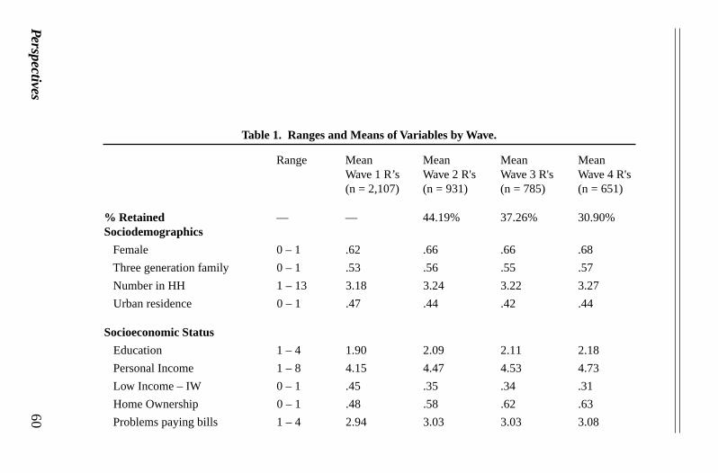
In Wolford and Torres’s (2001) paper, the authors showed a few examples of the waysin which the NSBA sample is affected through attrition. In Table 1, we provide moredetails on this issue. More specifically, we report mean levels of the variables used inthe attrition analyses across all four waves of the sample. We would expect that if theattrition across the waves was completely random, the means for each of the variableswould remain virtually unchanged. Note that the means reported for each wave arethe means of the first wave variables for those remaining in each wave.

As one can see looking across the table, the means of the variables do indeed changeas the sample becomes more reduced in size. For example, in terms ofsociodemographic factors, the sample becomes more female and rural over time. Re-garding socioeconomic status, the sample rises appreciably in terms of education andincome. Indeed, the proportion of the sample owning homes between waves one andfour rises by fifteen percentage points. We also note large changes in employmentstatus across the four waves. Likewise, some changes in community involvement areapparent, such as voting rates increase as does church activity and support of a Blackplatform. In short, across all sets of factors used to predict attrition, we observechanges in mean levels indicating fundamental changes in the composition of thesample.

The implications of the change in sample composition are twofold. First, it is readilyapparent that by the fourth wave, and indeed even the second, the sample is no longerrepresentative of the population from which it was drawn. Unfortunately, this prob-lem cannot be resolved using sample selection methods; however, other techniques,such as weighting, could reduce the problem of representativeness. Second, and moreimportantly for our purposes, the changes indicate that the attrition has been non-random. That is, it has been patterned in a variety of ways. Unless we take accountof these selection patterns in our analyses of the latter waves of data, biased andinconsistent estimates are possible (Breen 1996).

Predictors of All-cause Attrition

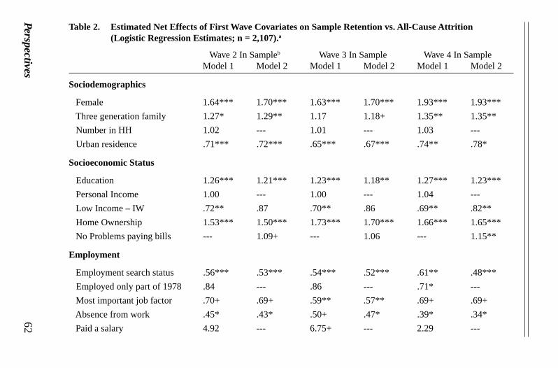
Most researchers using the NSBA data will be concerned with all-cause attrition, thatis, attrition from both mortality and non-mortality sources. Because the attrition modelsmust take account of all attrition to function correctly, these are the most appropriateoutcomes to model. We show the results of these models in Table 2. All of thevariables in the sociodemographics, socioeconomic status, employment, and com-munity involvement sections were those used in Wolford and Torres’s (2001) final

Perspectives60

Range Mean Mean Mean MeanWave 1 R’s Wave 2 R's Wave 3 R's Wave 4 R's(n = 2,107) (n = 931) (n = 785) (n = 651)

% Retained — — 44.19% 37.26% 30.90%Sociodemographics

Female 0 – 1 .62 .66 .66 .68

Three generation family 0 – 1 .53 .56 .55 .57

Number in HH 1 – 13 3.18 3.24 3.22 3.27

Urban residence 0 – 1 .47 .44 .42 .44

Socioeconomic Status

Education 1 – 4 1.90 2.09 2.11 2.18

Personal Income 1 – 8 4.15 4.47 4.53 4.73

Low Income – IW 0 – 1 .45 .35 .34 .31

Home Ownership 0 – 1 .48 .58 .62 .63

Problems paying bills 1 – 4 2.94 3.03 3.03 3.08

Table 1. Ranges and Means of Variables by Wave.

Perspectives61

Table 1 (continued). Ranges and Means of Variables by Wave.

Range Mean Mean Mean MeanWave 1 R’s Wave 2 R's Wave 3 R's Wave 4 R's(n = 2,107) (n = 931) (n = 785) (n = 651)

Employment

Employment search status 0 – 1 .42 .31 .30 .27

Employed only part of 1978 0 – 1 .56 .46 .45 .41

Most important job factor 0 – 1 .07 .06 .06 .06

Absence from work 0 – 1 .02 .01 .01 .01

Paid a salary 0 – 1 .00 .01 .01 .01

Community Involvement

Voted in presidential election 0 – 1 .54 .63 .64 .66

Church Activity 0 – 1 .18 .21 .23 .23

Supports Black Platform 0 – 1 .62 .68 .69 .71

Interviewer Observations

Asked interview length – IW 0 – 1 .22 .18 .16 .15

Difficulty with words – IW 0 – 1 .14 .11 .09 .08

Reluctant to sign re-contact – IW 0 – 1 .04 .02 .02 .02

Major repairs needed – IW 0 – 1 .17 .11 .10 .10

Minor repairs needed – IW 0 – 1 .35 .30 .29 .27

Physical problems – IW 0 – 1 .10 .05 .05 .05

Perspectives62

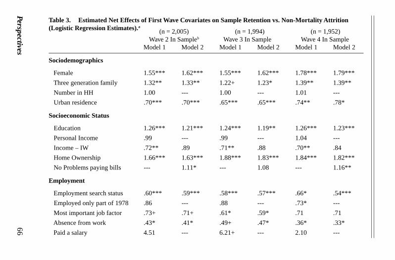
Wave 2 In Sampleb Wave 3 In Sample Wave 4 In SampleModel 1 Model 2 Model 1 Model 2 Model 1 Model 2

Sociodemographics

Female 1.64*** 1.70*** 1.63*** 1.70*** 1.93*** 1.93***

Three generation family 1.27* 1.29** 1.17 1.18+ 1.35** 1.35**

Number in HH 1.02 --- 1.01 --- 1.03 ---

Urban residence .71*** .72*** .65*** .67*** .74** .78*

Socioeconomic Status

Education 1.26*** 1.21*** 1.23*** 1.18** 1.27*** 1.23***

Personal Income 1.00 --- 1.00 --- 1.04 ---

Low Income – IW .72** .87 .70** .86 .69** .82**

Home Ownership 1.53*** 1.50*** 1.73*** 1.70*** 1.66*** 1.65***

No Problems paying bills --- 1.09+ --- 1.06 --- 1.15**

Employment

Employment search status .56*** .53*** .54*** .52*** .61** .48***

Employed only part of 1978 .84 --- .86 --- .71* ---

Most important job factor .70+ .69+ .59** .57** .69+ .69+

Absence from work .45* .43* .50+ .47* .39* .34*

Paid a salary 4.92 --- 6.75+ --- 2.29 ---

Table 2. Estimated Net Effects of First Wave Covariates on Sample Retention vs. All-Cause Attrition(Logistic Regression Estimates; n = 2,107).a

Perspectives 63

models, except for problems with bills in the socioeconomic section. We add thatvariable as well as the interviewer observations near the bottom of the table to themodels. In the first two columns, we regress retention (i.e., respondents coded one ifthey were in the sample at the second wave and zero otherwise) on the Wolford andTorres variables. According to this model, we find a number of significant predictorsof retention, notably home ownership, urban residence, and employment search sta-tus. Note that the estimates shown are odds ratios, meaning that values over one areindicative of greater retention based on higher levels of the predictor variable. Forexample, respondents who are home owners in the first wave are about 53% morelikely to be in the second wave sample than those who do not own homes in the firstwave. Similarly, women are more likely to be retained than men, as are those who aremore educated and who voted in the presidential election. In contrast, people livingin urban areas and those with low interviewer ratings of income were less likely to beretained. Looking at the fit statistics of this model, we note that the model explainsabout 12% of the variance in the dependent variable and is able to accurately predictcases about 69.9% of the time.

In the second column we present a similar model to the first but remove several vari-ables and add others, notably the interviewer observations. The variables we chosefor exclusion in the second model were those that were not significant predictors ofretention across more than one of the outcomes in either the all-cause or non-mortal-ity attrition cases. These variables include number in household, personal income,employed only part of 1978, paid a salary, and supports Black platform. Even thoughwe add several variables, with these subtractions the degrees of freedom used by themodel only increases by two. Looking at the estimates in the second column we notethat all except church activity and difficulty with words are significant predictors ofretention. The estimates of the Wolford and Torres variables do not change substan-tially, although in some cases, such as gender and voting, they do change somewhat.Among the new variables, respondents who had no problems paying bills were morelikely to be retained. In contrast, those who asked about the interview length, werereluctant to sign the re-contact form, who had physical problems, or who lived inpremises in need of repair were all less likely to be retained in the second wave.

Although these new variables are significant predictors themselves, it is important todetermine whether they actually improve the overall fit and predictive power of themodel. Looking at the fit statistics in column two, we see some improvement ismade. The change in chi-square (D X2 = 49.67) is significant, indicating better modelfit. The change in R2 reflects that the model explains slightly more variance. Further,the new model is better able to accurately predict retention by about 1.8%. In sumthen, the second model is an improvement over the first and entails little loss in parsi-mony.

Perspectives64

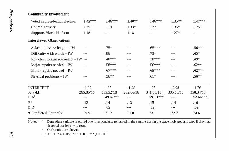
Community Involvement

Voted in presidential election 1.42*** 1.46*** 1.40** 1.46*** 1.35** 1.47***

Church Activity 1.25+ 1.19 1.33* 1.27+ 1.36* 1.25+

Supports Black Platform 1.18 --- 1.18 --- 1.27* ---

Interviewer Observations

Asked interview length – IW --- .75* --- .65*** --- .56***

Difficulty with words – IW --- .86 --- .73+ --- .65*

Reluctant to sign re-contact – IW --- .40*** --- .30*** --- .49*

Major repairs needed – IW --- .58*** --- .56*** --- .62**

Minor repairs needed – IW --- .67*** --- .65*** --- .62***

Physical problems – IW --- .56** --- .61* --- .56**

INTERCEPT -1.02 -.85 -1.28 -.97 -2.08 -1.76X2 / d.f. 265.85/16 315.52/18 282.66/16 341.85/18 305.68/16 358.34/18D X2 --- 49.67*** --- 59.19*** --- 52.66***

R2 .12 .14 .13 .15 .14 .16D R2 --- .02 --- .02 --- .02

% Predicted Correctly 69.9 71.7 71.0 73.1 72.7 74.6

Notes: a Dependent variable is scored one if respondents remained in the sample during the wave indicated and zero if they haddropped out for any reason.

b Odds ratios are shown.+ p < .10; * p < .05; ** p < .01; *** p < .001

Perspectives 65

The second and third sets of models follow the same patterns as those shown for thefirst. That is, both the Wolford and Torres and new variables all predict retention inthe third and fourth waves in fairly the same fashion as in the second wave. However,the changes in the models made in the third and fourth waves incur somewhat greaterfit and precision than that in the second wave. That is, in the third wave, the newmodel incurs a change of 59.19 in X2 and about 2.1% in accurate prediction. Thenumbers are similar for the fourth wave (D X2 = 52.66; prediction = +1.9%). In sum,for all-cause attrition, the changes we have made to the models do provide better fitand predictive ability. Further, given that the interviewer variables are unlikely tooverlap with variables used in a substantive model, the new model could be applied ina number of situations to predict attrition.1

Non-mortality Attrition

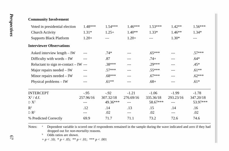
In Table 3 we display the results of the non-mortality attrition models. The estimatedeffects shown in these models are very similar to those shown for the all-cause attri-tion models. This similarity should not be surprising given that a large majority of thesample attrition is due to non-mortality causes. Like the all-cause mortality models,the most powerful predictors of non-mortality attrition are SES factors such as educa-tion and home ownership and some of the interviewer observations. Likewise, themodel fit statistics and changes between the Wolford and Torres models and our ownare similar. Consequently, in the interest of conserving space, we do not furtherdiscuss the pattern of these findings.

Distress Example

In Table 4 we display the results of our distress example. In the first column, wereport the effects of the first wave covariates on fourth wave distress modeled usingordinary least squares regression. Note that our choice of variables in this examplewas theoretically derived only to the extent that we wanted to find a set of variablesthat would have some effect on the fourth wave outcome. Consequently, we chosevariables along several dimensions known to influence distress, such as gender, so-cioeconomic status, prior mental health problems, current physical health problems,self-esteem, and religious activity. Very few of these variables overlap with the vari-

1 We considered the possibility that self-reported health problems would predict attrition giventhat some of the attrition is likely due to mortality or an incapacity to participate. Conse-quently, we examined whether the health measure used in the distress example also predictedattrition. We found that in both the all-cause and non-mortality cause attrition models, thisindex had no significant effect. This non-significant finding for self-reported health under-scores the utility of the interviewer observations, especially for health problems.

Perspectives66

(n = 2,005) (n = 1,994) (n = 1,952) Wave 2 In Sampleb Wave 3 In Sample Wave 4 In Sample

Model 1 Model 2 Model 1 Model 2 Model 1 Model 2

Sociodemographics

Female 1.55*** 1.62*** 1.55*** 1.62*** 1.78*** 1.79***

Three generation family 1.32** 1.33** 1.22+ 1.23* 1.39** 1.39**

Number in HH 1.00 --- 1.00 --- 1.01 ---

Urban residence .70*** .70*** .65*** .65*** .74** .78*

Socioeconomic Status

Education 1.26*** 1.21*** 1.24*** 1.19** 1.26*** 1.23***

Personal Income .99 --- .99 --- 1.04 ---

Income – IW .72** .89 .71** .88 .70** .84

Home Ownership 1.66*** 1.63*** 1.88*** 1.83*** 1.84*** 1.82***

No Problems paying bills --- 1.11* --- 1.08 --- 1.16**

Employment

Employment search status .60*** .59*** .58*** .57*** .66* .54***

Employed only part of 1978 .86 --- .88 --- .73* ---

Most important job factor .73+ .71+ .61* .59* .71 .71

Absence from work .43* .41* .49+ .47* .36* .33*

Paid a salary 4.51 --- 6.21+ --- 2.10 ---

Table 3. Estimated Net Effects of First Wave Covariates on Sample Retention vs. Non-Mortality Attrition(Logistic Regression Estimates).a

Perspectives67

Community Involvement

Voted in presidential election 1.48*** 1.54*** 1.46*** 1.53*** 1.42** 1.56***

Church Activity 1.31* 1.25+ 1.40** 1.33* 1.46** 1.34*

Supports Black Platform 1.20+ --- 1.20+ --- 1.30* ---

Interviewer Observations

Asked interview length – IW --- .74* --- .65*** --- .57***

Difficulty with words – IW --- .87 --- .74+ --- .64*

Reluctant to sign re-contact – IW --- .38*** --- .29*** --- .45*

Major repairs needed – IW --- .57*** --- .55*** --- .61**

Minor repairs needed – IW --- .68*** --- .67*** --- .62***

Physical problems – IW --- .61** --- .68+ --- .61*

INTERCEPT -.95 -.92 -1.21 -1.06 -1.99 -1.78X2 / d.f. 257.96/16 307.32/18 276.69/16 335.36/18 293.23/16 347.20/18D X2 --- 49.36*** --- 58.67*** --- 53.97***

R2 .12 .14 .13 .15 .14 .16D R2 --- .02 --- .02 --- .02

% Predicted Correctly 69.9 71.7 71.1 73.2 72.6 74.6

Notes: a Dependent variable is scored one if respondents remained in the sample during the wave indicated and zero if they haddropped out for non-mortality reasons.

b Odds ratios are shown.+ p < .10; * p < .05; ** p < .01; *** p < .001

Perspectives 68

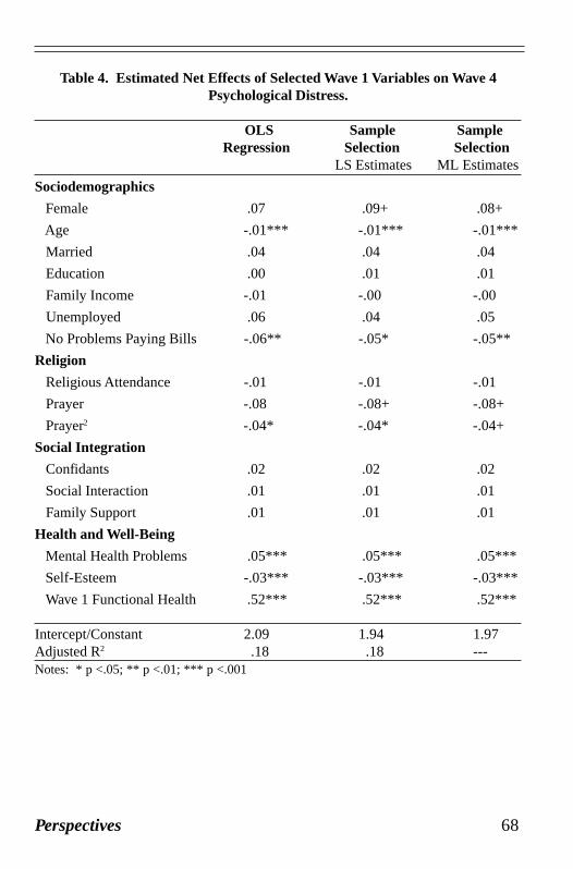
Table 4. Estimated Net Effects of Selected Wave 1 Variables on Wave 4Psychological Distress.

OLS Sample Sample Regression Selection Selection LS Estimates ML Estimates

Sociodemographics

Female .07 .09+ .08+

Age -.01*** -.01*** -.01***

Married .04 .04 .04

Education .00 .01 .01

Family Income -.01 -.00 -.00

Unemployed .06 .04 .05

No Problems Paying Bills -.06** -.05* -.05**

Religion

Religious Attendance -.01 -.01 -.01

Prayer -.08 -.08+ -.08+

Prayer2 -.04* -.04* -.04+

Social Integration

Confidants .02 .02 .02

Social Interaction .01 .01 .01

Family Support .01 .01 .01

Health and Well-Being

Mental Health Problems .05*** .05*** .05***

Self-Esteem -.03*** -.03*** -.03***

Wave 1 Functional Health .52*** .52*** .52***

Intercept/Constant 2.09 1.94 1.97Adjusted R2 .18 .18 ---Notes: * p <.05; ** p <.01; *** p <.001

Perspectives 69

ables in the attrition models; consequently, we can be certain that our attrition modelsare having the intended effect.

In Table 4 we display the results of the distress models. In the first model we reportthe estimates from an uncorrected ordinary least squares regression model. In thesecond column we show the estimates generated from a Heckman two-step least squaressample selection model, while in the third the estimates are derived from a sampleselection model with maximum likelihood estimation. According to Breen (1996)the latter of these models tends to provide the best estimates of the population param-eters.

In comparing coefficients across the models, we note one important pattern: verylittle change is evidenced through the incorporation of the sample selection analyses.Indeed, only three effect sizes, those for gender, income, and employment status,changed between the first and latter two models. Although the effect of gender be-came significant (p < .05) in the sample selection models, the absolute change incoefficient size was small (D b = .02). Another variable, the squared form of prayer,dropped slightly in significance. However, overall, incorporating the selection mod-els had very little effect on the analyses.

Discussion

Our analyses revealed three important findings. First, the attrition in the NSBA overthe four waves is nonrandom; consequently, analyses using latter waves of the samplemay be biased unless the nonrandom attrition is accounted for. It should be noted thatthe approximate 8 to 9 year gap between the first and second waves of the NSBAlargely accounts for the exceptionally high level of attrition in wave 2. This long gapexacerbates the already difficult process of relocating respondents that is experiencedby all longitudinal surveys. It suggests that new data collection efforts that anticipateany form of follow-up interviewing should plan to recontact respondents over shorterperiods of time. Second, the inclusion of interviewer observations is important forthe prediction of attrition. Further, because these variables will not often be used insubstantive analyses, they will not face the problem of overlap with other variablesthat are often used. Our findings also suggest that interviewers are fairly skilled atrecognizing potential problems with certain respondents. Given declining participa-tion and cooperation rates in all surveys including those with face-to-face interviews,these analyses suggest the need for additional research regarding the dynamics ofinterview processes. Finally, even though the attrition is non-random, once it is takeninto consideration, the coefficient estimates in our example change very little.

Generally speaking, we found several groups of factors to be predictive of attrition inthis sample. One of the strongest sets of predictors involved socioeconomic status

Perspectives 70

measured in several ways. For instance, we found across both forms of attrition andall waves that education, and especially home ownership, were strong predictors ofattrition. These findings support our assertion that those SES factors promote stabil-ity and perhaps a willingness to advance the goals of the study. Severalsociodemographic variables were also predictive, notably gender and urban residence.With regard to gender, it is somewhat unclear why women were less likely to drop outof the sample. In order to better understand this finding, we examined the actualreasons for attrition during the second wave, which had the largest amount of attri-tion. In reviewing these reasons by gender, we noted that 12.6% of men but only8.9% of women were not recontacted due to the “too ill/circumstantial” reason cat-egory. Based on this difference, it may be the case that men were sicker than womenat later waves. Likewise, other analyses show that men were more likely to have died(men: 10.9%, women: 6.0%). However, it might also be the case that men wereprevented from participating more often than women due to incarceration. Data fromthe Department of Justice (Snell 1995) supports this assertion showing that the incar-ceration rate as of 1993 for Black men was 4.63% compared to only .24% for Blackwomen.2 In short, it appears that the differences in attrition we observe are either dueto health reasons, death, or some other incapacitation, such as incarceration.

The final set of factors showing great utility for predicting attrition are the interviewerobservations. Several of these factors, notably home repair status, physical problems,and reluctance to sign the re-contact sheet were strong predictors of attrition. Indeed,the addition of these factors significantly improved the overall fit and predictive abil-ity of the model. These findings buttress the few studies that have profitably usedthese measures in the past. They further suggest that future studies on health andother outcomes should consider their usage both in terms of modeling substantiveoutcomes and/or selection.

At this point, readers might question whether engaging these models is worth theeffort for outcomes such as distress or other factors commonly analyzed by behav-ioral scientists. Indeed, the time involved in undertaking these models for research-ers not already familiar with them would be non-negligible. So then, is it worth theeffort to undertake these models? In our opinion, it is. As more and more data setsbecome longitudinal, researchers, and manuscript reviewers, are becoming increas-ingly sensitive to issues of sample attrition. Consequently, even though accountingfor attrition may yield little effect, readers will want to know that such analyses wereundertaken to rule out the possibility of those effects. Likewise, even though we did

2 Our estimates of incarceration rates were based on 1993 incarceration figures reported in theSnell (1995) report and the population size for African American men and women aged eigh-teen and older as reported in the 1990 census.

Perspectives 71

not find substantial differences in our own example, differences can exist. Withoutproper analytical techniques being applied, these differences could go undiscoveredleading to erroneous findings and conclusions.

Acknowledgements

The authors would like to thank Rachel Deckler with her assistance in manuscriptpreparation. Address correspondence to Marc A. Musick, Population Research Cen-ter, MAI 1800, The University of Texas at Austin, Austin, TX 78712 (email:musick@prc.utexas.edu).

References

Beggs, John J., Valerie A. Haines, and Jeanne S. Hurlbert. 1996. “Revisiting the Ru-ral-Urban Contrast: Personal Networks in Nonmetropolitan and Metropolitan Set-tings.” Rural Sociology 61(2):306-325.

Breen, Richard. 1996. Regression Models: Censored, Sample Selected, or TruncatedData. Thousand Oaks, CA: Sage.

Ellison, Christopher G. 1992. “Are Religious People Nice People? Evidence from theNational Survey of Black Americans.” Social Forces 71:411-430.

Ellison, Christopher G. 1993. “Religious Involvement and Self-Perception amongBlack Americans.” Social Forces 71:1027-1055.

Ellison, Christopher G., and Darren E. Sherkat. 1990. “Patterns of Religious MobilityAmong Black Americans.” The Sociological Quarterly 31:551-568.

Ellison, Christopher G., Jeffrey S. Levin, Robert J. Taylor, and Linda M. Chatters.1997. “The Effects of Religious Attendance, Guidance, and Support on Psychologi-cal Distress: Longitudinal Findings from the National Survey of Black Americans.”Paper presented at the annual meetings of the Society for the Scientific Study ofReligion, San Diego.

Greiner, P.A., D.A. Snowdon, and L.H. Greiner. 1996. “The Relationship of Self-Rated Function and Self-Rated Health to Concurrent Functional Ability, FunctionalDecline, and Mortality: Findings from the Nun Study.” Journal of Gerontology: So-cial Sciences 46:55-65.

Heckman, James J. 1979. “Sample Selection Bias as a Specification Error.”Econometrica 47:153-161.

Perspectives 72

House, James S., Cynthia Robbins, and Helen L. Metzner. 1982. “The Association ofSocial Relationships and Activities with Mortality: Prospective Evidence from theTecumseh Community Health Study.” American Journal of Epidemiology 116:123-14.

Hughes, Michael, and Bradley R. Hertel. 1990. “The Significance of Color Remains:A Study of Life Chances, Mate Selection, and Ethnic Consciousness Among BlackAmericans.” Social Forces 68:1105-1120.

Hummer, Robert A., Richard G. Rogers, Charles B. Nam, and Christopher G. Ellison.1999. “Religious Involvement and U.S. Adult Mortality.” Demography 36:273-285.

Idler, Ellen L., and Stanislav Kasl. 1991. “Health Perceptions and Survival: Do Glo-bal Evaluations of Health Status Really Predict Mortality?” Journal of Gerontology:Social Sciences 46:S55-S65.

Idler, Ellen L., and Yael Benyamini. 1997. “Self-Rated Health and Mortality: A Re-view of Twenty-Seven Community Studies.” Journal of Health and Social Behavior38:21-37.

Jackson, James S., and Gerald Gurin. 1997. National Survey of Black Americans,Waves 1-4, 1979-1980, 1987-1988, 1988-1989, 1992 [Computer file]. Conducted byUniversity of Michigan, Survey Research Center. ICPSR version Ann Arbor, MI:Inter-university Consortium for Political and Social Research [producer and distribu-tor].

Jackson, J.S., T.B. Brown, D.R. Williams, M.E. Torres, S.L. Sellers, and K.B. Brown.1996. ‘’Racism and the Physical and Mental Health Status of African Americans: A13-Year National Panel Study.’’ Ethnicity and Disease 6:132-147.

Johnson, Ernest H., and Clifford L. Broman. 1987. “The Relationship of Anger Ex-pression to Health Problems among Black Americans in a National Survey.” Journalof Behavioral Medicine 10:103-116.

Kaplan, George A. 1996. “People and Places: Contrasting Perspectives on the Asso-ciation Between Social Class and Health.” International Journal of Health Services26:507-519.

Keith, Verna M., and Cedric Herring. 1991. “Skin Tone and Stratification in the BlackCommunity.” American Journal of Sociology 97:760-768.

Lantz, Paula M. and James S. House, James M. Lepkowski, David R. Williams, Rich-

Perspectives 73

ard P. Mero, and Jieming Chen. 1998. “Socioeconomic Status, Health Behaviors, andMortality: Results from a Nationally-Representative Prospective Study of U.S. Adults.”Journal of the American Medical Association 279:1703-1708.

Lewis, Edith A. 1989. “Role Strain in African-American Women: The Efficacy ofSupport Networks.” Journal of Black Studies 20:155-169.

Moen, Phyllis, Donna Dempster-McClain, and Robin M. Williams, Jr. 1989. “SocialIntegration and Longevity: An Event History Analysis of Women’s Roles and Resil-ience.” American Sociological Review 54:635-647.

Musick, Marc A., A. Regula Herzog, and James S. House. 1999. “Volunteering andMortality Among Older Adults: Findings From A National Sample.” Journal of Ger-ontology: Social Sciences 54:S173-S180.

Neighbors, Harold W. 1985. “Seeking Professional Help for Personal Problems: BlackAmericans’ Use of Health and Mental Health Services.” Community Mental HealthJournal 21:156-166.

Neighbors, Harold W., James S. Jackson, Phillip J. Bowman, and Gerald Gurin. 1983.“Stress, Coping and Black Mental Health: Preliminary Findings from a National Study.”Prevention in Human Services 2:5-29.

Neighbors, Harold W., Marc A. Musick, and David R. Williams. 1998. “African Ameri-can Ministers as a Source of Help for Serious Personal Crises: Bridge or Barrier toMental Health Care?” Health Education and Behavior 25:759-777.

Pappas, G., S. Queen, W. Hadden, and G. Fisher. 1993. “The Increasing Disparity inMortality Between Socioeconomic Groups in the United States, 1960 and 1986.”New England Journal of Medicine 329:103-109.

Rogers, Richard G., Robert A. Hummer, and Charles B. Nam. 2000. Living and Dy-ing in the USA: Behavioral, Health and Social Differentials of Adult Mortality. SanDiego: Academic Press.

Sherkat, Darren E., and Christopher G. Ellison. 1991. “The Politics of Black Reli-gious Change: Disaffiliation from Black Mainline Denominations.” Social Forces70:431-454.

Smith, G.D., C. Hart, D. Hole, P. MacKinnon, C. Gillis, G. Watt, D. Blane, and V.Hawthorne. 1998. “Education and Occupational Social Class: Which Is the MoreImportant Indicator of Mortality Risk?” Journal of Epidemiology and Community

Perspectives 74

Health 52:153-160.

Smith, Mark H., Roger T. Anderson, Douglas D. Bradham, and Charles F. Longino,Jr. 1995. “Rural and Urban Differences in Mortality Among Americans 55 Years andOlder: Analysis of the National Longitudinal Mortality Study.” The Journal of RuralHealth 11:274-285.

Snell, Tracy L. 1995. Correctional Populations in the United States, 1993. Bureau ofJustice Statistics (NCJ-156241).

Sorlie, P.D., E. Backlund, and J.B. Keller. 1995. “U.S. Mortality by Economic, De-mographic, and Social Characteristics: The National Longitudinal Mortality Study.”American Journal of Public Health 85:949-956.

Stolzenberg, Ross M., and Daniel A. Relles. 1997. “Tools for Intuition About SampleSelection Bias and Its Correction.” American Sociological Review 62:494-507.

Strawbridge, William J., Richard D. Cohen, Sarah J. Shema, and George A. Kaplan.1997. “Frequent Attendance at Religious Services and Mortality Over 28 Years.”American Journal of Public Health 87:957-961.

Taylor, Robert J., and Linda M. Chatters. 1986. “Patterns of Informal Support toElderly Black Adults: Family, Friends, and Church Members.” Social Work 31:432-438.

Taylor, Robert J., Harold W. Neighbors, and Clifford L. Broman. 1989. “Evaluationby Black Americans of the Social Service Encounter during a Serious Social Prob-lem.” Social Work 34:205-211.

Taylor, Robert J., and Linda M. Chatters. 1991. “Extended Family Networks of OlderBlack Adults.” Social Sciences 46:S210-217.

Wilson, John, and Marc Musick. 1997. “Who Cares? Toward an Integrated Theory ofVolunteer Work.” American Sociological Review 62:694-713.

Wolford, Monica L., and Myriam Torres. 2001. “Nonresponse Adjustment in a Lon-gitudinal Survey of African Americans.” African American Research Perspectives7:37-49.

Wolinsky, Fredric D., and Robert J. Johnson. 1992. “Perceived Health Status andMortality Among Older Men and Women.” Journal of Gerontology: Social Sciences47:S304-S312.