Transversal structures on triangulations: A combinatorial study and straight-line drawings

Discrete Mathematics 309 (2009) 1870–1894www.elsevier.com/locate/disc

Transversal structures on triangulations: A combinatorial study andstraight-line drawings

Eric Fusy

Algorithms Project, INRIA Rocquencourt and LIX, Ecole Polytechnique, France

Received 9 February 2006; accepted 27 December 2007Available online 4 March 2008

Abstract

This article focuses on a combinatorial structure specific to triangulated plane graphs with quadrangular outer face and noseparating triangle, which are called irreducible triangulations. The structure has been introduced by Xin He under the name ofregular edge-labelling and consists of two bipolar orientations that are transversal. For this reason, the terminology used here isthat of transversal structures. The main results obtained in the article are a bijection between irreducible triangulations and ternarytrees, and a straight-line drawing algorithm for irreducible triangulations. For a random irreducible triangulation with n vertices,the grid size of the drawing is asymptotically with high probability 11n/27×11n/27 up to an additive error of O(

√n). In contrast,

the best previously known algorithm for these triangulations only guarantees a grid size (dn/2e − 1)× bn/2c.c© 2008 Elsevier B.V. All rights reserved.

Keywords: Triangulations; Bipolar orientations; Bijection; Straight-line drawing

1. Introduction

A plane graph, or planar map, is a connected graph embedded in the plane without edge-crossings, and consideredup to orientation-preserving homeomorphism. Many drawing algorithms for plane graphs [1,4,9,12,18,20,27] endowthe graph with a particular structure, from which coordinates are assigned to vertices in a natural way. For example,triangulations, i.e., plane graphs with only triangular faces, are characterized by the fact that their inner edges canbe partitioned into three spanning trees with specific incidence relations, the so-called Schnyder woods [27]. Thesespanning trees yield a natural method for assigning coordinates to a vertex, by counting the number of faces in specificregions. Placing the vertices accordingly on an integer grid and linking adjacent vertices by segments yields a straight-line drawing algorithm, which can be refined to produce a drawing on an integer grid (n − 2) × (n − 2), with n thenumber of vertices; see [4,28].

In this article we focus on so-called irreducible triangulations, which are plane graphs with quadrangular outer face,triangular inner faces, and no separating triangle, i.e., each 3-cycle is the boundary of a face. Irreducible triangulationsform an important class of triangulations, as they are closely related to 4-connected triangulations. In addition, asdiscussed in [3], many plane graphs, including bipartite plane graphs and 4-connected plane graphs with at least fourouter vertices, can be triangulated into an irreducible triangulation. There exist more compact straight-line drawing

E-mail address: [email protected].

0012-365X/$ - see front matter c© 2008 Elsevier B.V. All rights reserved.doi:10.1016/j.disc.2007.12.093

http://www.elsevier.com/locate/disc

mailto:[email protected]

http://dx.doi.org/10.1016/j.disc.2007.12.093

E. Fusy / Discrete Mathematics 309 (2009) 1870–1894 1871

algorithms for irreducible triangulations [19,22], the size of the grid being guaranteed to be (dn/2e − 1) × bn/2c inthe worst case. By investigating a bijection with ternary trees, we have observed that each irreducible triangulationT can be endowed with a so-called transversal structure, which can be summarized as follows. Naming as W , N ,E , S (like West, North, East, South) the four outer vertices of T in clockwise order, the inner edges of T can beoriented and partitioned into two sets: red edges that “flow” from S to N , and blue edges that “flow” from W to E .As we learned after completing a first draft of this paper, X. He [18] has defined the same structure under the nameof regular edge-labelling, and derived a nice algorithm of rectangular-dual drawing, which has been recently appliedto the theory of cartograms [8,29]. We give two equivalent definitions of transversal structures in Section 2: onewithout orientations called a transversal edge-partition, and one with orientations called a transversal pair of bipolarorientations (which corresponds to the regular edge-labelling of X. He). Transversal structures characterize irreducibletriangulations in the same way as Schnyder woods characterize triangulations, and they share similar combinatorialproperties. In particular, we show in Section 3 that the set of transversal structures of an irreducible triangulation is adistributive lattice, and that the “flip” operation has a simple geometric interpretation (Theorem 2).

The transversal structure at the bottom of the lattice, called minimal, has a strong combinatorial role, as it allows usto establish a bijection between ternary trees and irreducible triangulations. The bijection, called the closure mapping,is described in Section 4. The mapping from ternary trees to irreducible triangulations relies on “closure operations”,as introduced by G. Schaeffer in his PhD [25]; see also [17,24]. This bijection has in fact brought about our discoveryof transversal edge-partitions, as a natural edge-bicoloration of a ternary tree is mapped to the minimal transversaledge-partition of the associated triangulation (similarly, the bijection of [24] maps the structure of Schnyder woods).Classical algorithmic applications of bijections between trees and plane graphs are random generation – as detailedin [25,26] – and encoding algorithms for plane graphs – as detailed in [17,24] – with application to mesh compressionin computational geometry. The closure mapping presented in this article yields linear time procedures for randomsampling (under a fixed-size uniform distribution) and optimal encoding (in the information theoretic sense) of 4-connected triangulations. These algorithms are described in the thesis of the author [16]. The focus in this article(besides the graph drawing algorithm) is on the application to counting; the bijection yields a combinatorial way toenumerate rooted 4-connected triangulations, which were already counted by Tutte in [30] using algebraic methods.

In Section 5, we derive from transversal structures a straight-line drawing algorithm for irreducible triangulations.Like for algorithms using Schnyder woods [4,27], the drawing is obtained by using face-counting operations. Ouralgorithm outputs a straight-line drawing on an integer grid of half-perimeter n − 1 if the triangulation has n vertices(Theorem 5). This is to be compared with previous algorithms for irreducible triangulations by He [19] and Miuraet al. [22]. The latter produces a grid (dn/2e − 1) × bn/2c; the half-perimeter is also n − 1, but the aspect ratio ofthe outer face is better. However, the algorithms of [19] and [22] rely on a particular order for treating the vertices,the canonical ordering, and a step of coordinate-shifting makes them difficult to implement and to carry out by hand.In contrast, our algorithm can readily be performed on a piece of paper, because the coordinates of the vertices arecomputed independently with simple face-counting operations.

Furthermore, some coordinate-deletions can be performed on the drawing obtained using the face-countingalgorithm, with the effect of reducing the size of the grid (Theorem 6). For an irreducible triangulation with n verticestaken uniformly at random and endowed with its minimal transversal structure (for the distributive lattice), we showin Section 6 (Theorem 7) that the size of the grid after coordinate-deletions is asymptotically with high probability11n/27×11n/27 up to an additive error of order

√n. Compared to [19] and [22], we do not improve on the size of the

grid in the worst case, but we improve asymptotically with high probability by a reduction factor 27/22 on the widthand height of the grid; see Fig. 12 for an example. The proof of the grid size 11n/27× 11n/27 makes use of severalingredients: a combinatorial interpretation of coordinate-deletions, the bijection with ternary trees, and modern toolsof analytic combinatorics such as the quasi-power theorem [14].

The following diagram summarizes the connections between the different combinatorial structures and the rolethey play for the drawing algorithms.

1872 E. Fusy / Discrete Mathematics 309 (2009) 1870–1894

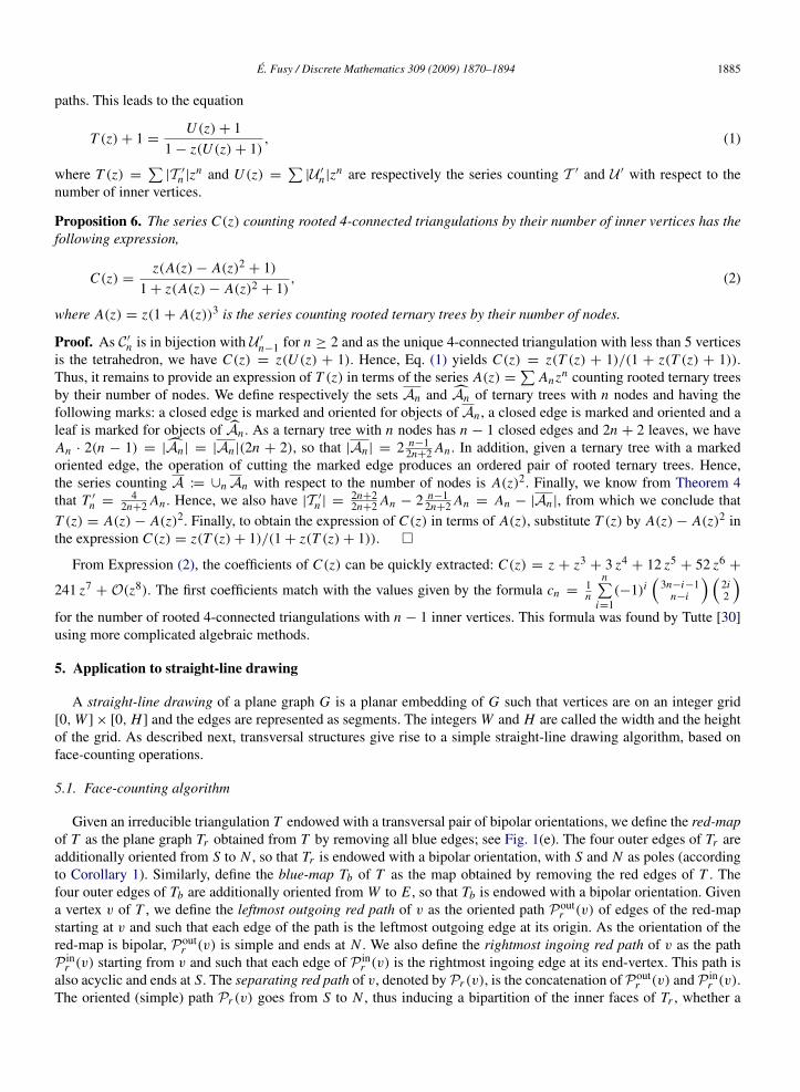
Fig. 1. Transversal edge-partition: local condition (a) and a complete example (b). In parallel, the transversal pair of bipolar orientations: localcondition (c) and a complete example (d) with the two induced bipolar orientations (e).

2. Transversal structures: Definitions

In this section we give two definitions of transversal structures, one without orientations called the transversal edge-partition and one with orientations called the transversal pair of bipolar orientations. As we will prove in Proposition 2,the two definitions are in fact equivalent, i.e., the additional information given by the orientations is redundant. Thedefinition without orientations is more convenient for the combinatorial study (lattice property and bijection withternary trees), while the definition with orientations fits better for describing the straight-line drawing algorithm inSection 5.

2.1. Transversal edge-partition

Let T be an irreducible triangulation. Edges and vertices of T are said to be inner or outer according to whetherthey are incident to the outer face or not. A transversal edge-partition of T is a combinatorial structure where eachinner edge of T is given a color – red or blue – such that the following conditions are satisfied.

C1 (Inner vertices): In clockwise order around each inner vertex v, the edges incident to v form: a non-empty intervalof red edges, a non-empty interval of blue edges, a non-empty interval of red edges, and a non-empty intervalof blue edges; see Fig. 1(a).

C2 (Outer vertices): Writing a1, a2, a3, a4 for the outer vertices of T in clockwise order, all inner edges incident toa1 and to a3 are of one color and all inner edges incident to a2 and to a4 are of the other color.

An example of transversal edge-partition is illustrated in Fig. 1(b), where red edges are DARK GREY and blue edgesare LIGHT GREY (the same convention will be used for all figures).

2.2. Transversal pair of bipolar orientations

An orientation of a graph G is said to be acyclic if it has no oriented circuit (a circuit is an oriented simple cycleof edges). Given an acyclic orientation of G, a vertex having no ingoing edge is called a source, and a vertex havingno outgoing edge is called a sink. A bipolar orientation is an acyclic orientation with a unique source, denoted s anda unique sink, denoted t . Such an orientation is also characterized by the fact that, for each vertex v 6= {s, t}, thereexists an oriented path from s to t passing by v; see [10] for a detailed discussion. An important property of a bipolarorientation on a plane graph is that the edges incident to a vertex v 6= {s, t} are partitioned into a non-empty intervalof ingoing edges and a non-empty interval of outgoing edges; and, dually, each face f of M has two particular verticess f and t f such that the boundary of f consists of two non-empty oriented paths both going from s f to t f , the pathwith f on its right (left) is called the left lateral path (right lateral path, resp.) of f .

Let T be an irreducible triangulation. Call N , E , S and W the four outer vertices of T in clockwise order aroundthe outer face. A transversal pair of bipolar orientations of T is a combinatorial structure where each inner edge ofT is given a direction and a color – red or blue – such that the following conditions are satisfied (see Fig. 1(d) for anexample):

C1’ (Inner vertices): In clockwise order around each inner vertex v of T , the edges incident to v form: a non-emptyinterval of outgoing red edges, a non-empty interval of outgoing blue edges, a non-empty interval of ingoingred edges, and a non-empty interval of ingoing blue edges; see Fig. 1(c).


C2’ (Outer vertices): All inner edges incident to N , E , S and W are respectively ingoing red, ingoing blue, outgoingred, and outgoing blue.

This structure is also considered in [18,20] under the name of regular edge-labelling.

Proposition 1. The orientation of the edges given by a transversal pair of bipolar orientation is acyclic. The sourcesare W and S, and the sinks are E and N.

Proof. Let T be an irreducible triangulation endowed with a transversal pair of bipolar orientations. Assume thereexists a circuit, and consider a minimal one C, i.e., the interior of C is not included in the interior of any other circuit.It is easy to check from Condition C2’ that C is not the boundary of a face of T . Thus the interior of C contains at leastone edge e incident to a vertex v of C. Assume that e is going out of v. Starting from e, it is always possible, whenreaching a vertex inside C, to go out of that vertex toward one of its neighbours. Indeed, a vertex inside C is an innervertex of T , and hence has positive outdegree according to Condition C1’. Thus, there is an oriented path startingfrom e, that either loops C into a circuit in the interior of C – impossible by minimality of C – or reaches C again —impossible as a chordal path for C would yield two smaller circuits. Thus, the orientation is acyclic. Finally ConditionC1’ ensures that no inner vertex of T can be a source or a sink, and Condition C2’ ensures that W and S are sources,and E and N are sinks. �

The following corollary of Proposition 1, also proved in [18], explains the name transversal pair of bipolarorientations; see also Fig. 1(e).

Corollary 1 ([18]). Let T be an irreducible triangulation endowed with a transversal pair of bipolar orientation.Then the (oriented) red edges induce a bipolar orientation of the plane graph obtained from T by removing W , E,and all non-red edges. Similarly, the blue edges induce a bipolar orientation of the plane graph obtained from T bydeleting S, N , and all non-blue edges.

3. The lattice property of transversal edge-partitions

We investigate the set E(T ) of transversal edge-partitions of a fixed irreducible triangulation T . Kant and He [20]have shown that E(T ) is not empty and that an element of E(T ) can be computed in linear time. In this section, weprove that E(T ) is a distributive lattice. This property is to be compared with the lattice property of other similarcombinatorial structures on plane graphs, such as bipolar orientations [23] and Schnyder woods [6,13]. Our prooftakes advantage of the property that the set of orientations of a plane graph with a prescribed outdegree for eachvertex is a distributive lattice. To apply this result to transversal edge-partitions, we establish a bijection betweenE(T ) and some orientations with prescribed vertex outdegrees on an associated plane graph, called the angular graphof T .

3.1. Lattice structure of α-orientations on a plane graph

Let us first recall the definition of a distributive lattice. A lattice is a partially ordered set (E,≤) such that, for eachpair (x, y) of elements of E , there exists a unique element x ∧ y and a unique element x ∨ y satisfying the conditions:

• x ∧ y ≤ x , x ∧ y ≤ y, and ∀z ∈ E , z ≤ x and z ≤ y implies z ≤ x ∧ y,• x ∨ y ≥ x , x ∨ y ≥ y, and ∀z ∈ E , z ≥ x and z ≥ y implies z ≥ x ∨ y.

In other words, each pair admits a unique common lower element dominating all other common lower elements,and the same holds with common upper elements. The lattice is said to be distributive if the operators ∧ and ∨ aredistributive with respect to each other, i.e., ∀(x, y, z) ∈ E , x∧(y∨z) = (x∧y)∨(x∧z) and x∨(y∧z) = (x∨y)∧(x∨z).The nice feature of distributive lattices is that, in most cases, moving from an element of the lattice to a covering lower(upper) element has a simple geometric interpretation, which we informally call a flip (flop). As we recall next, in thecase of orientations of a plane graph with prescribed vertex outdegrees, the flip (flop) operation consists in reversinga clockwise circuit (counterclockwise circuit).

Given a plane graph G = (V, E), and a function α : V → N, an α-orientation of G is an orientation of G suchthat each vertex v of G has outdegree α(v). An oriented circuit C is called essential if it has no chordal path (a chordalpath is an oriented path of edges in the interior of C with the two extremities on C).


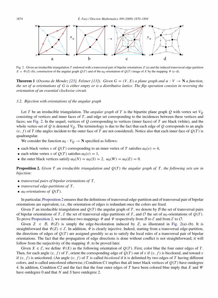
Fig. 2. Given an irreducible triangulation T endowed with a transversal pair of bipolar orientations Z (a) and the induced transversal edge-partitionE = Φ(Z) (b), construction of the angular graph Q(T ) and of the α0-orientation of Q(T ) image of E by the mapping Ψ (c–d).

Theorem 1 (Ossona de Mendez [23], Felsner [13]). Given G = (V, E) a plane graph and α : V → N a function,the set of α-orientations of G is either empty or is a distributive lattice. The flip operation consists in reversing theorientation of an essential clockwise circuit.

3.2. Bijection with orientations of the angular graph

Let T be an irreducible triangulation. The angular graph of T is the bipartite plane graph Q with vertex set VQconsisting of vertices and inner faces of T , and edge set corresponding to the incidences between these vertices andfaces; see Fig. 2. In the sequel, vertices of Q corresponding to vertices (inner faces) of T are black (white), and thewhole vertex-set of Q is denoted VQ . The terminology is due to the fact that each edge of Q corresponds to an angle(v, f ) of T (the angles incident to the outer face of T are not considered). Notice also that each inner face of Q(T ) isquadrangular.

We consider the function α0 : VQ → N specified as follows:

• each black vertex v of Q(T ) corresponding to an inner vertex of T satisfies α0(v) = 4,• each white vertex v of Q(T ) satisfies α0(v) = 1,• the outer black vertices satisfy α0(N ) = α0(S) = 2, α0(W ) = α0(E) = 0.

Proposition 2. Given T an irreducible triangulation and Q(T ) the angular graph of T , the following sets are inbijection:

• transversal pairs of bipolar orientations of T ,• transversal edge-partitions of T ,• α0-orientations of Q(T ).

In particular, Proposition 2 ensures that the definitions of transversal edge-partition and of transversal pair of bipolarorientations are equivalent, i.e., the orientation of edges is redundant once the colors are fixed.

Given T an irreducible triangulation and Q(T ) the angular graph of T , we denote by B the set of transversal pairsof bipolar orientations of T , E the set of transversal edge-partitions of T , and O the set of α0-orientations of Q(T ).To prove Proposition 2, we introduce two mappings Φ and Ψ respectively from B to E and from E to O.

Given Z ∈ B, Φ(Z) is simply the edge-bicoloration induced by Z , as illustrated in Fig. 2(a)–(b). It isstraightforward that Φ(Z) ∈ E . In addition, Φ is clearly injective. Indeed, starting from a transversal edge-partition,the directions of edges of Q(T ) are assigned greedily so as to satisfy the local rules of a transversal pair of bipolarorientations. The fact that the propagation of edge directions is done without conflict is not straightforward; it willfollow from the surjectivity of the mapping Φ, to be proved later.

Given X ∈ E , we define Ψ(X) as the following orientation of Q(T ). First, color blue the four outer edges of T .Then, for each angle (v, f ) of T , orient the corresponding edge of Q(T ) out of v if (v, f ) is bicolored, and toward vif (v, f ) is unicolored. (An angle (v, f ) of T is called bicolored if it is delimited by two edges of T having differentcolors, and is called unicolored otherwise.) Condition C1 implies that all inner black vertices of Q(T ) have outdegree4. In addition, Condition C2 and the fact that the four outer edges of T have been colored blue imply that E and Whave outdegree 0 and that N and S have outdegree 2.


The following lemma ensures that all white vertices have outdegree 1 in Ψ(X), so that Ψ(X) is an α0-orientation.

Lemma 1. Let T be a plane graph with quadrangular outer face, triangular inner faces, and endowed with atransversal edge-partition, the four outer edges being additionally colored blue. Then there is no mono-colored innerface, i.e., each inner face of T has two sides of one color and one side of the other color.

Proof. Let Λ be the number of bicolored angles of T and let n be the number of inner vertices of T . ConditionC1 implies that there are 4n bicolored angles incident to an inner vertex of T . Condition C2 and the fact that allouter edges are colored blue imply that two angles incident to N and two angles incident to S are bicolored. Hence,Λ = 4n + 4.

Moreover, as T has a quadrangular outer face and triangular inner faces, Euler’s relation ensures that T has 2n+ 2inner faces. For each inner face, two cases can arise: either the three sides have the same color, or two sides are ofone color and one side is of the other color. In the first (second) case, the face has 0 (2) bicolored angles. As there are2n + 2 inner faces and Λ = 4n + 4, the pigeonhole principle implies that all inner faces make a contribution of 2 tothe number of bicolored angles, which concludes the proof. �

Lemma 1 ensures that Ψ is a mapping from E to O. In addition, it is clear that Ψ is injective. To prove Proposition 2,it remains to prove that Φ and Ψ are surjective. As Φ is injective, it is sufficient to show that Ψ ◦Φ is surjective. Thus,given O ∈ O, we have to find Z ∈ B such that Ψ ◦ Φ(Z) = O .

Computing the preimage of an α0-orientation. We now describe a method for computing a transversal pair ofbipolar orientations Z consistent with a given α0-orientation O , i.e., such that Ψ ◦ Φ(Z) = O . The algorithm makesuse of a sweeping process to orient and color the inner edges of T ; a simple (i.e., not self-intersecting) path P of inneredges of T going from W to E is maintained, the path moving progressively toward the vertex S (at the end, the pathis P = W → S→ E). We require that the following invariants are satisfied throughout the sweeping process.

(1) Each vertex of P \ {W, E} has two outgoing edges on each side of P for the α0-orientation O .(2) The inner edges of T already oriented and colored are those on the left of P .(3) Condition C1’ holds around each inner vertex of T on the left of P .(4) A partial version of C1’ holds around each vertex v of P \ {W, E}. The edges incident to v on the left of P form

in clockwise order: a possibly empty interval of ingoing blue edges, a non-empty interval of outgoing red edges,and a possibly empty interval of outgoing blue edges.

(5) All edges already oriented and colored and incident to N , E , S, W are ingoing red, ingoing blue, outgoing red,and outgoing blue, respectively.

(6) The edges of T already colored (and oriented) are consistent with the α0-orientation O , i.e., for each angle (v, f )delimited by two edges of T already colored, the corresponding edge of Q(T ) is going out of v iff the angle isbicolored.

At first we need a technical result ensuring that Invariant (1) is sufficient for a path to be simple.

Lemma 2. Let T be an irreducible triangulation and Q(T ) be the angular graph of T , endowed with an α0-orientation O. Let P be a path of inner edges of T from W to E such that each vertex of P \ {W, E} has outdegree 2on each side of P for the α0-orientation. Then the path P is simple.

Proof. Assume that the path P loops into a circuit; and consider an inclusion-minimal such circuit C =

(v0, v1, . . . , vk = v0). We define n•, n◦ and e as the numbers of black vertices (i.e., vertices of T ), white verticesand edges of Q(T ) inside C. As T is triangulated and C has length k, Euler’s relation ensures that T has 2n• + k − 2faces inside C, i.e., n◦ = 2n• + k − 2. Counting the edges of Q(T ) inside C according to their incident white vertexgives (i): e = 3n◦ = 6n• + 3k − 6. The edges of Q(T ) inside C can also be counted according to their origin for theα0-orientation. Each vertex of C – except possibly the self-intersection vertex v0 – has outdegree 2 in the interior of Cfor the α0-orientation. Hence, (ii): e = 4n• + n◦ + 2k − 2+ δ = 6n• + 3k − 4+ δ, where δ ≥ 0 is the outdegree ofv0 inside C. Taking (ii)− (i) yields δ = −2, a contradiction. �

The path P is initialized with all neighbours of N , from W to E . In addition, all inner edges incident to N areinitially colored red and directed toward N ; see Fig. 5(b). The invariants (1)–(6) are clearly true at the initial step.


Fig. 3. An admissible pair v, v′ of vertices, and the matching path P(v, v′).

Fig. 4. The update step of the iterative algorithm to find the preimage of an α0-orientation.

Let us introduce some terminology in order to describe the sweeping process. Throughout the process, the verticesof P are ordered from left to right, with W as leftmost and E as rightmost vertex. Given v, v′ a pair of vertices on P –with v on the left of v′ – the part of P going from v to v′ is denoted by [v, v′]. For each vertex w on P , let f1, . . . , fkbe the sequence of faces of T incident to w on the right of P , taken in counterclockwise order. The edge of Q(T )associated with the angle (w, f1) (angle (w, fk)) is denoted by εleft(w) (by εright(w), resp.). A pair of vertices v, v′ onP – with v on the left of v′ – is called admissible if εright(v) is ingoing at v, εleft(v

′) is ingoing at v′, and for each vertexw ∈ [v, v′] \ {v, v′}, the edges εleft(w) and εright(w) are going out of w. Clearly an admissible pair always exists: takea pair v, v′ of vertices on P that satisfy {εright(v) ingoing at v, εleft(v

′) ingoing at v′} and are closest possible. Noticethat two vertices v, v′ forming an admissible pair are not neighbours on P (otherwise the white vertex associatedwith the face on the right of [v, v′] would have outdegree > 1). Let w0 = v,w1, . . . , wk, wk+1 = v′ (k ≥ 1) bethe sequence of vertices of [v, v′]. The matching path of v, v′ is the path of edges of T that starts at v, visits theneighbours of w1, w2, . . . , wk on the right of P , and finishes at v′. The matching path of v, v′ is denoted by P(v, v′).Let P ′ be the path obtained from P when substituting [v, v′] by P(v, v′). As shown in Fig. 3, the path P ′ goes fromW to E and each vertex of P ′ \ {W, E} has outdegree 2 on each side of P ′ for the α0-orientation O . Hence the path P ′is simple according to Lemma 2. Moreover, by definition of P(v, v′), all edges of T in the region enclosed by [v, v′]and P(v, v′) connect a vertex of [v, v′] \ {v, v′} to a vertex of P(v, v′) \ {v, v′}; see Fig. 4.

We can now describe the operations performed at each step of the sweeping process, as shown in Fig. 4.

• Choose an admissible pair v, v′ of vertices on P .• Color blue and orient from left to right all edges of [v, v′].• Color red all edges inside the area enclosed by [v, v′] and P(v, v′), and orient these edges from P(v, v′) to [v, v′].• Update the path P , the part [v, v′] being replaced by P(v, v′).

According to the discussion above, the path P is still simple after these operations, and satisfies Invariant (1).All the other invariants (2)–(6) are easily shown to remain satisfied, as illustrated in Fig. 4. At the end, the path Pis equal to W → S → E . The invariants (3) and (5) ensure that the directions and colors of the inner edges of Tform a transversal pair of bipolar orientations Z ; and Invariant (6) ensures that Z is consistent with the α0-orientationO , i.e., Ψ ◦ Φ(Z) = O; see also Fig. 5 for a complete execution of the algorithm. This concludes the proof ofProposition 2.

3.3. Essential circuits of an α0-orientation

Proposition 2 ensures that the set E of transversal edge-partitions of an irreducible triangulation is a distributivelattice, as E is in bijection with the distributive lattice formed by the α0-orientations of the angular graph. By definition,the flip operation on E is the effect of a flip operation on O via the bijection. Recall that a flip operation on an α-orientation consists in reversing a clockwise essential circuit (circuit with no chordal path). Hence, to describe the flipoperation on E , we have to characterize the essential circuits of an α0-orientation. For this purpose, we introduce theconcept of straight path.

Consider an irreducible triangulation T endowed with a transversal pair of bipolar orientations. Color blue the fourouter edges of T and orient them from W to E . The conditions C1’ and C2’ ensure that there are four possible typesfor a bicolored angle (e, e′) of T , with e′ following e in cw order: (outgoing red, outgoing blue) or (outgoing blue,ingoing red) or (ingoing red, ingoing blue) or (ingoing blue, outgoing red). The type of an edge of Q(T ) corresponding


Fig. 5. The complete execution of the algorithm calculating the preimage of an α0-orientation O . At each step, the vertices of the matching pathP(v, v′) are surrounded.

to a bicolored angle of T (i.e., an edge going out of a black vertex) is defined as the type of the bicolored angle. Forsuch an edge e, the straight path of e is the oriented path P of edges of Q(T ) that starts at e and such that each edgeof P going out of a black vertex has the same type as e. Such a path is unique, as there is a unique choice for theoutgoing edge at a white vertex (each white vertex has outdegree 1).

Lemma 3. The straight path P of an edge e ∈ Q(T ) going out of a black vertex is simple and ends at an outer blackvertex of Q(T ).

Proof. Notice that the conditions of a transversal pair of bipolar orientations remain satisfied if the directions of theedges of one color are reversed and then the colors of all inner edges are switched; hence the edge e can be assumedto have type (outgoing red, outgoing blue) without loss of generality. Let v0, v1, v2, . . . , vi , . . . be the sequence ofvertices of the straight path P of e, so that the even indices correspond to black vertices of Q(T ) and the odd indicescorrespond to white vertices of Q(T ). Observe that, for k ≥ 0, the black vertices v2k and v2k+2 are adjacent inT and the edge (v2k, v2k+2) is either outgoing red or outgoing blue. Hence (v0, v2, v4, . . . , v2k, . . .) is an orientedpath of T , so that it is simple, according to Proposition 1. Hence, P does not pass twice by the same black vertex,i.e., v2k 6= v2k+2 for k 6= k′; and P neither passes twice by the same white vertex (otherwise v2k+1 = v2k+3 for k 6= k′

would imply v2k+2 = v2k+4 by unicity of the outgoing edge at each white vertex, a contradiction). Thus P is a simplepath, so that it ends at a black vertex of Q(T ) having no outgoing edge of type (outgoing red, outgoing blue), i.e., Pends at an outer black vertex of Q(T ). �

Proposition 3. Given T an irreducible triangulation and Q(T ) its angular graph endowed with an α0-orientation X,an essential clockwise circuit C of X satisfies either of the two following configurations:

• The circuit C is the boundary of a (quadrangular) inner face of Q(T ); see Fig. 6(a).• The circuit C has length 8. The four black vertices of C have no outgoing edge inside C. The four white vertices of

C have their unique incident edge not on C inside C; see Fig. 6(b) for an example.

Proof. First we claim that no edge of Q(T ) inside C has its origin on C; indeed the straight path construction ensuresthat such an edge could be extended to a chordal path of C, which is impossible. We define n•, n◦ and e as the numberof black vertices, white vertices and edges inside C. We denote by 2k the number of vertices on C, so that there are kblack and k white vertices on C. Euler’s relation and the fact that all inner faces of Q(T ) are quadrangular ensure that(i): e = 2(n•+n◦)+k−2. As each white vertex of Q(T ) has degree 3, a white vertex on C has a unique incident edgenot on C. Let l be the number of white vertices such that this incident edge is inside C (notice that l ≤ k). Counting theedges inside C according to their incident white vertex gives (ii): e = 3n◦ + l. The edges inside C can also be countedaccording to their origin for the α0-orientation. As no edge inside C has its origin on C, we have (iii) : e = 4n• + n◦.


Fig. 6. The two possible configurations of an essential clockwise circuit C of Q(T ). In each case, an alternating 4-cycle is associated with thecircuit; and reversing the circuit orientation corresponds to switching the edge colors inside the alternating 4-cycle.

Taking 2(i)− (ii)− (iii) yields l = 2k − 4. As k is a positive integer and l is a non-negative integer satisfying l ≤ k,the only possible values for l and k are {k = 4, l = 4}, {k = 3, l = 2}, and {k = 2, l = 0}. It is easily seen that thecase {k = 3, l = 2} would correspond to a separating 3-cycle. Hence, the only possible cases are {k = 2, l = 0} and{k = 4, l = 4}, shown in Fig. 6(a) and (b), respectively. The first case corresponds to a circuit of length 4, which hasto be the boundary of a face, as the angular graph of an irreducible triangulation (more generally, of a 3-connectedplane graph) is well known to have no filled 4-cycle. �

3.4. Flip operation on transversal structures

As we prove now, the essential circuits of α0-orientations correspond to specific patterns on transversal structures,making it possible to have a simple geometric interpretation of the flip operation, formulated directly on the transversalstructure.

Given T an irreducible triangulation endowed with a transversal edge-partition, we define an alternating 4-cycleas a cycle C = (e1, e2, e3, e4) of four edges of T that are color-alternating (i.e., two adjacent edges of C have differentcolors). Given a vertex v on C, we name as the left-edge (right-edge) of v the edge of C starting from v and having theexterior of C on its left (on its right).

Lemma 4. An alternating 4-cycle C in a transversal structure satisfies either of the two following configurations.• All edges inside C and incident to a vertex v of C have the color of the left-edge of v. Then C is called

a left alternating 4-cycle• All edges inside C and incident to a vertex v of C have the color of the right-edge of v. Then C is called

a right alternating 4-cycle.

Proof. Let k be the number of vertices inside C. Condition C1 ensures that there are 4k bicolored angles incident to avertex inside C. Moreover, Euler’s relation ensures that there are 2k + 2 faces inside C. Hence Lemma 1 implies thatthere are 4k+ 4 bicolored angles inside C. As a consequence, there are four bicolored angles inside C that are incidentto a vertex of C. As C is alternating, each of the four vertices of C is incident to at least one bicolored angle. Hence thepigeonhole principle implies that each vertex of C is incident to one bicolored angle inside C. Moreover, each of thefour inner faces ( f1, f2, f3, f4) inside C and incident to an edge of C has two bicolored angles, according to Lemma 1.As such a face fi has two angles incident to vertices of C, at least one bicolored angle of fi is incident to a vertexof C. As there are four bicolored angles inside C incident to vertices of C, the pigeonhole principle ensures that eachface f1, f2, f3, f4 has exactly one bicolored angle incident to a vertex of C. As each vertex of C is incident to onebicolored angle inside C, these angles are in the same direction. If they start from C in clockwise (counterclockwise)direction, then C is a right alternating 4-cycle (left alternating 4-cycle). �

Theorem 2. The set of transversal edge-partitions of a fixed irreducible triangulation is a distributive lattice. Theflip operation consists in switching the edge-colors inside a right alternating 4-cycle, turning it into a left alternating4-cycle.


Fig. 7. The execution of the closure mapping on an example.

Proof. The two possible configurations for an essential clockwise circuit of an α0-orientation are representedrespectively in Fig. 6(a) and (b). In each case, the essential circuit of the angular graph corresponds to a rightalternating 4-cycle on T . Notice that a clockwise face of Q(T ) corresponds to the vertex-empty alternating 4-cycle,whereas essential circuits of length 8 correspond to all possible alternating 4-cycles with at least one vertex in theirinterior (Fig. 6(a) gives an example). As shown in Fig. 6, the effect of reversing a clockwise essential circuit of theangular graph is clearly a color switch of the edges inside the associated alternating 4-cycle. �

Definition. Given an irreducible triangulation T , the transversal structure of T with no right alternating 4-cycle iscalled minimal, as it is at the bottom of the distributive lattice.

4. Bijection with ternary trees

This section focuses on the description of a bijection between ternary trees and irreducible dissections, wherethe minimal transversal structure (for the distributive lattice) plays a crucial role. The mapping from ternary trees toirreducible triangulations relies on so-called closure operations, as introduced by G. Schaeffer in his PhD [25].

4.1. The closure mapping: From trees to triangulations

A plane tree is a plane graph with a unique face (the outer face). A ternary tree is a plane tree with vertex degreesin {1, 4}. Vertices of degree 4 are called nodes and vertices of degree 1 are called leaves. An edge of a ternary tree iscalled a closed edge if it connects two nodes and is called a stem if it connects a node and a leaf. It will be convenientto consider closed edges as made of two opposite half-edges meeting at the middle of the edge, whereas stems will beconsidered as made of a unique half-edge incident to the node and having not (yet) an opposite half-edge. A ternarytree is rooted by marking one leaf. The root allows us to distinguish the four neighbours of each node, taken in ccworder, into a parent (the neighbour in the direction of the root), a left-child, a middle-child, and a right-child. Thus, ourdefinition of rooted ternary trees corresponds to the classical definition, where each node has three ordered children.

Starting from a ternary tree, the three steps to construct an irreducible triangulation are: local closure, partial closureand complete closure. Perform a counterclockwise walk alongside a ternary tree A (imagine an ant walking around Awith the infinite face on its right). If a stem s and then two sides of closed edges e1 and e2 are successively encounteredduring the traversal, create a half-edge opposite to the stem s and incident to the farthest extremity of e2, so as to losea triangular face. This operation is called a local closure; see the transition Fig. 7(a)–(b).

The figure obtained in this way differs from A by the presence of a triangular face and, more importantly, a stems of A has become a closed edge, i.e., an edge made of two half-edges. Each time a sequence (stem, closed edge,closed edge) is found ccw around the outer face of the current figure, we perform a local closure, update the figure,and restart, until no local closure is possible. This greedy execution of local closures is called the partial closure of A;see Fig. 7(c). It is easily shown that the figure F obtained by performing the partial closure of A does not depend onthe order of execution of the local closures. Indeed, a cyclic parenthesis word is associated with the counterclockwisewalk alongside the tree, with an opening parenthesis of weight 2 for a stem and a closing parenthesis for a side ofclosed edge; the future local closures correspond to matchings of the parenthesis word.


At the end of the partial closure, the number ns of unmatched stems and the number ne of sides of closed edgesincident to the outer face of F satisfy the relation ns − ne = 4. Indeed, this relation is satisfied on A because a ternarytree with n nodes has n − 1 closed edges and 2n + 2 leaves (as proved by induction on the number of nodes); and therelation ns − ne = 4 remains satisfied throughout the partial closure, as each local closure decreases ns and ne by 1.When no local closure is possible anymore, two consecutive unmatched stems on the boundary of the outer face of Fare separated by at most one closed edge. Hence, the relation ns = ne + 4 implies that the unmatched stems of F arepartitioned into four intervals I1, I2, I3, I4, where two consecutive stems of an interval are separated by one closededge, and the last stem of Ii is incident to the same vertex as the first stem of I(i+1)mod 4; see Fig. 7(c).

The last step of the closure mapping, called complete closure, consists of the following operations. Draw a 4-gon(v1, v2, v3, v4) outside of F ; for i ∈ {1, 2, 3, 4}, create an opposite half-edge for each stem s of the interval Ii , the newhalf-edge being incident to the vertex vi . Clearly, this process creates only triangular faces, so it yields a triangulationof the 4-gon; see Fig. 7(d).

Let us now explain how the closure mapping is related to transversal edge-partitions. A ternary tree A is said to beedge-bicolored if each edge of A (closed edge or stem) is given a color – red or blue – such that any angle incident toa node of A is bicolored; see Fig. 7(a). Such a bicoloration, which is unique up to the choice of the colors, is calledthe edge-bicoloration of A.

Lemma 5. Let A be a ternary tree endowed with its edge-bicoloration. The following invariant is maintainedthroughout the partial closure of A,

(I ): any angle incident to the outer face of the current figure is bicolored.

Proof. By definition of the edge-bicoloration, (I ) is true on A. We claim that (I ) remains satisfied after each localclosure. Indeed, let (s, e1, e2) be the succession (stem, closed edge, closed edge) intervening in the local closure, let vbe the extremity of e2 farthest from s, and let e3 be the ccw follower of e2 around v. Invariant (I ) implies that s ande2 have the same color. As we give to the new created half-edge h the same color as its opposite half-edge s (in orderto have unicolored edges), h and e2 have the same color. The effect of the local closure on the angles of the outerface is the following: the angle (e1, e2) disappears from the outer face, and the angle (e2, e3) is replaced by the angle(h, e3). As e2 has the same color as h, the bicolored angle (e2, e3) is replaced by the bicolored angle (h, e3), so that(I ) remains true after the local closure. �

It also follows from this proof that Condition C1 remains satisfied throughout the partial closure, because thenumber of bicolored angles around each node is not increased, and is initially equal to 4. At the end of the partialclosure, Invariant (I ) ensures that all stems of the intervals I1 and I3 are of one color, and all stems of the intervalsI2 and I4 are of the other color. Hence, Condition C2 is satisfied after the complete closure; see Fig. 7(d). Thus, theclosure maps the edge-bicoloration of A to a transversal edge-partition of the obtained triangulation of the 4-gon,which is in fact the minimal one:

Proposition 4. The closure of a ternary tree A with n nodes is an irreducible triangulation T with n inner vertices.The closure maps the edge-bicoloration of A to the minimal transversal edge-partition of T .

Proof. Assume that T has a separating 3-cycle C. Observe that Lemma 1 was stated and proved without theirreducibility condition. Hence, when the four outer edges of T are colored blue, each inner face of T has exactlytwo bicolored angles. Let k ≥ 1 be the number of vertices inside C. Euler’s relation implies that the interior of Ccontains 2k + 1 faces, so that there are 4k + 2 bicolored angles inside C, according to Lemma 1. Moreover, ConditionC1 implies that there are 4k bicolored angles incident to a vertex that is in the interior of C. Hence there are exactlytwo bicolored angles inside C incident to a vertex of C. However, for each of the three edges {e1, e2, e3} of C, the faceincident to ei in the interior of C has at least one of its two bicolored angles incident to ei . Hence, there are at leastthree bicolored angles inside C and incident to a vertex of C, a contradiction.

Now we show that the transversal edge-partition of T induced by the closure mapping is minimal, i.e., has no rightalternating 4-cycle. Let C be an alternating 4-cycle of T . This cycle has been closed during a local closure involvingone of the four edges of C. Let e be this edge and let v be the origin of the stem whose completion has created theedge e. The fact that the closure of a stem is always performed with the infinite face on its right ensures that e is theright-edge of v on C, as defined in Section 3.4. A second observation following from Invariant (I ) is that, when a stem


Fig. 8. The opening algorithm performed on an example.

s is merged, the angle formed by s and by the edge following s in counterclockwise order around the origin of s is abicolored angle. This ensures that C is a left alternating 4-cycle. �

4.2. Inverse mapping: The opening

In this section, we describe the inverse of the closure mapping, from irreducible triangulations to ternary trees. Aswe have seen in the proof of Lemma 5, during a local closure, the newly created half-edge h has the same color as theclockwise-consecutive half-edge around the origin of h. Hence, for each half-edge h incident to an inner vertex of T ,

• if the angle formed by h and its cw-consecutive half-edge is unicolored, then h has been created during a localclosure,• if the angle is bicolored, then h is one of the 4 original half-edges of A incident to v.

This property indicates how to inverse the closure mapping. Given an irreducible triangulation T , the opening ofT consists of the following steps, illustrated in Fig. 8.

(1) Endow T with its minimal transversal edge-partition.(2) Remove the outer quadrangle of T and all half-edges of T incident to a vertex of the quadrangle.(3) Remove all the half-edges whose clockwise-consecutive half-edge has the same color.

The following lemma is a direct consequence of the definition of the opening mapping:

Lemma 6. Let A be a ternary tree and let T be the irreducible triangulation obtained by performing the closure ofA. Then the opening of T is A.

Hence, the closure Φ and the opening Ψ are such that Ψ ◦ Φ = Id. To prove that the opening and the closuremapping are mutually inverse, it remains to prove that Φ ◦Ψ = Id, which is more difficult and is done in two steps:

(1) Show that the opening of an irreducible triangulation T is a ternary tree,(2) Show that the closure of this ternary tree is T .

The first step is to define an orientation of the half-edges of T induced by the minimal transversal edge-partition.Each half-edge of T is associated with the angle on its right (looking from the incident vertex). We orient half-edgesof T toward (outward of) their incident vertex if the associated angle is unicolored (bicolored); with the restrictionthat half-edges on the outer quadrangle are left unoriented and all angles incident to an outer vertex are considered asunicolored. This yields an orientation of the half-edges of T , which is called the 4-orientation of T . Each inner vertexof T is incident to four bicolored angle, hence has outdegree 4 in the 4-orientation. By definition of the 4-orientation,the opening of an irreducible triangulation consists in removing the outer 4-gon and all ingoing half-edges.

Let e be an inner edge of T . An important remark is that the two half-edges of e can not be simultaneously directedtoward their respective incident vertex (otherwise, the 4-cycle C bordering the two triangular faces incident to e wouldbe a right alternating 4-cycle, a contradiction).

Hence, only two cases arise for an inner edge e of T .

• If one half-edge of e is ingoing, then e is called a stem-edge. A stem-edge can be considered as simply oriented(both half-edges have the same direction) for the 4-orientation.


Fig. 9. The existence of a clockwise circuit in the 4-orientation of T implies the existence of a clockwise circuit in the minimal α0-orientation ofQ(T ).

• If the two half-edges of e are outgoing, then e is called a tree-edge. A tree-edge can be considered as a bi-orientededge for the 4-orientation.

We define a clockwise circuit of the 4-orientation of T as a simple cycle C of inner edges of T such that each edgeof C is either a tree-edge (i.e., a bi-oriented edge) or a stem-edge having the interior of C on its right.

Lemma 7. The 4-orientation of T has no clockwise circuit.

Proof. Assume there exists a clockwise circuit C in the 4-orientation of T . For a vertex v on C, we denote by hvthe half-edge of C going out of v when doing a clockwise traversal of C, and by ev the edge of Q(T ) following hvin clockwise order around v (notice that ev is the most counterclockwise edge of Q(T ) incident to v inside C). AsC is a clockwise circuit for the 4-orientation of T , hv is directed outward of v. Hence the angle θ on the right ofhv is a bicolored angle for the minimal transversal edge-partition of T , so that ev is going out of v for the minimalα0-orientation Omin of Q(T ).

We use this observation to build iteratively a clockwise circuit of Omin (see Fig. 9), yielding a contradiction. Let v0be a vertex on C and P(v0) the straight path starting at ev0 , as defined in Section 3.3, for the minimal α0-orientationOmin of Q(T ). Lemma 3 ensures that P(v0) is simple and ends at an outer vertex of Q(T ). In particular, P(v0) hasto reach C at a vertex v1 different from v0. We denote by P1 the part of P(v0) between v0 and v1, by Λ1 the part of Cbetween v1 and v0, and by C1 the cycle obtained by concatenating P1 and Λ1. Let P(v1) be the straight path startingat ev1 . The fact that ev1 is the most counterclockwise incident edge of v1 in the interior of C ensures that P(v1) startsin the interior of C1. The path P(v1) has to reach C1 at a vertex v2 6= v1. We denote by P2 the part of P(v1) betweenv1 and v2. If v2 belongs to P1, then the concatenation of the part of P1 between v2 and v1 and of P2 is a clockwisecircuit of Omin, a contradiction. Hence v2 is on Λ1 strictly between v1 and v0. We denote by P2 the concatenation ofP1 and P2, and by Λ2 the part of C going from v2 to v0. As v2 is strictly between v1 and v0, Λ2 is strictly includedin Λ1. We denote by C2 the cycle made of the concatenation of P2 and Λ2. Similarly as for the path P(v1), the pathP(v2) must start in the interior of C2.

Then we continue iteratively; see Fig. 9. At each step k, we consider the straight path P(vk) starting at evk . Thispath starts in the interior of the cycle Ck , and reaches again Ck at a vertex vk+1. The vertex vk+1 can not belong toPk , otherwise a clockwise circuit of Omin would be created. Hence vk+1 is strictly between vk and v0 on C, i.e., is inΛk \ {vk, v0}. In particular the path Λk+1 going from vk+1 to v0 on C, is strictly included in the path Λk going from vkto v0 on C. Thus, Λk shrinks strictly at each step. Hence, there must be a step k0 where P(vk0) reaches Ck0 at a vertexon Pk0 , thus creating a clockwise circuit of Omin, a contradiction. �

Lemma 8. The tree-edges of T form a tree spanning the inner vertices of T .

Proof. Denote by H the graph consisting of the tree-edges of T and their incident vertices. A first observation is thatH has no cycle, as such a cycle of bi-oriented edges of T would be a clockwise circuit in the 4-orientation of T . Letn be the number of inner vertices of T . Observe that H can not be incident to the outer vertices of T , so that H can


cover at most the set of inner vertices of T . A well known result of graph theory ensures that an acyclic graph Hhaving n − 1 edges and covering a subset of an n-vertex set V is a tree covering exactly all vertices of V . Hence itremains to show that H has (n − 1) edges. Let s be the number of stem-edges and t be the number of tree-edges ofT . As T has n inner vertices, there are 4n outgoing half-edges in the 4-orientation of T . Moreover, each stem-edgehas contribution 1 and each tree-edge has contribution 2 to the number of outgoing half-edges. Hence, s + 2t = 4n.Finally, Euler’s relation ensures that T has (3n + 1) inner edges, so that s + t = 3n + 1. These two equalities ensurethat t = n − 1, which concludes the proof that H is a tree spanning the inner vertices. �

Lemma 9. The opening of an irreducible triangulation T is a ternary tree.

Proof. As we have seen from the definition of the 4-orientation, the opening of an irreducible triangulation consists inremoving the outer 4-gon and all ingoing half-edges. The figure obtained in this way consists of the tree-edges, whichform a spanning tree according to Lemma 8, and of the half-edges that have lost their opposite half-edge. The edgesof the first and second type correspond respectively to the closed edges and to the stems of the tree. In addition, afterremoving all ingoing half-edges, each vertex has degree 4, so that the tree satisfies the degree-conditions of a ternarytree. �

Lemma 10. Let T be an irreducible triangulation and let A be the ternary tree obtained by doing the opening of T .Then the closure of A is T .

Proof. First it is clear that the complete closure (transition between Fig. 7(c) and Fig. 7(d)) is the inverse of Step 2 ofthe opening algorithm. Let F be the figure obtained from T after Step 2 of the opening mapping.

To prove that the partial closure of A is F , it is sufficient to find a chronological order of deletion of the ingoinghalf-edges of F (for the 4-orientation) such that the inverse of each half-edge deletion is a local closure. A localclosure satisfies the property that the new created half-edge h has the outer face on its right when h is traversed towardits incident vertex. Thus the half-edge h chosen to be disconnected at step k must be incident to the outer face ofthe current figure Fk , with Fk on the right when h is traversed toward its incident vertex. We claim that there alwaysexists such a half-edge as long as there remain stem-edges in Fk . In that case, Fk contains the spanning tree H madeof the tree-edges of T plus at least one stem-edge. Hence Fk contains at least a cycle, thus a simple cycle C can beextracted from the boundary of Fk . There is at least one stem-edge e on C, because no cycle is formed by tree-edgesonly. We claim that e has the outer face of Fk on its right, so that the ingoing half-edge h of e is a candidate to bedeleted (indeed if e had the outer face of Fk on its left, the concatenation of e and of the path of tree-edges connectingthe two extremities of e would be a clockwise circuit in the 4-orientation, a contradiction). As discussed above, theinverse operation of the deletion of h is a local closure, which concludes the proof. �

Finally, Lemmas 6 and 10 yield the following theorem:

Theorem 3 (Bijection). For n ≥ 1, the closure mapping is a bijection between the set of ternary trees with n nodesand the set of irreducible triangulations with n inner vertices. The inverse mapping of the closure is the opening.

Theorem 4 (Bijection, Rooted Version). For n ≥ 1, the closure mapping induces a (2n + 2)-to-4 correspondencebetween the set A′n of rooted ternary trees with n nodes and the set T ′n of rooted irreducible triangulations with ninner vertices. In other words, A′n × {1, . . . , 4} is in bijection with T ′n × {1, . . . , 2n + 2}.

Proof. It can easily be proved by induction on the number of nodes that a ternary tree with n nodes has 2n + 2leaves. Hence, when rooting the ternary tree obtained by doing the opening of a triangulation in T ′n , there are 2n + 2possibilities to place the root. Conversely, starting from a rooted ternary tree with n nodes, there are four possibilitiesto place the root on the irreducible triangulation obtained by doing the closure of the tree, because the root has to beplaced on one of the four outer edges. �

4.3. Application to counting triangulations

In this section we focus on the application to exact enumeration. The key point is that the bijection reduces thetask of counting irreducible triangulations to the much easier task of counting ternary trees. Then, we show that theenumeration of irreducible triangulations naturally leads to the enumeration of rooted 4-connected triangulations,


which are closely related; the ingredients are generating functions and a decomposition of a rooted irreducibletriangulation as a sequence of rooted 4-connected triangulations.

4.3.1. Counting irreducible triangulationsAs a first direct application, the bijection with ternary trees yields counting formulas for irreducible triangulations.

Proposition 5 (Counting Irreducible Triangulations). For n ≥ 1, the number of rooted irreducible triangulationswith n inner vertices is

|T ′n | = 4(3n)!

n!(2n + 2)!.

The number of unrooted irreducible triangulations with n inner vertices is

|Tn| =(3n)!

n!(2n + 2)!+

12

(3k)!

k!(2k + 1)!if n ≡ 0 mod 2 [n = 2k],

|Tn| =(3n)!

n!(2n + 2)!+

12(3k + 1)!

k!(2k + 2)!+

12

(3k′)!

k′!(2k′ + 1)!if n ≡ 1 mod 4 [n = 2k + 1 = 4k′ + 1],

|Tn| =(3n)!

n!(2n + 2)!+

12(3k + 1)!

k!(2k + 2)!if n ≡ 3 mod 4 [n = 1+ 2k].

Proof. The enumerative formula follows from |T ′n | = 42n+2 |A′n| and from the well known fact that |A′n| =

(3n)!/((2n + 1)!n!), which can be derived from the Lagrange inversion formula applied to the generating functionA(z) = z(1+ A(z))3. The formula for |Tn| = |An| follows from the enumeration of unrooted ternary trees, which iseasily obtained by considering the possible rotation symmetries (order 2 around a vertex or an edge, order 4 around avertex). �

The formula for rooted irreducible triangulations can easily be obtained from the series counting rootedtriangulations of the 4-gon by using a composition scheme; see [30]. To our knowledge, the counting formulafor unrooted irreducible triangulations is new. However, a composition scheme should make it possible to countirreducible triangulations with a given rotation symmetry (order 2 around a vertex or an edge, order 4 around a vertex),starting from triangulations of the 4-gon with a given rotation symmetry, which have been counted by Brown [7].

4.3.2. Counting rooted 4-connected triangulationsA graph is said to be 4-connected if it has more than three vertices and if at least four vertices have to be removed

to disconnect it. In this section we derive the enumeration of rooted 4-connected triangulations from the countingformula for rooted irreducible triangulations. The idea is to translate a decomposition linking these two families ofrooted triangulations to an equation linking their generating functions. The net result we obtain is an explicit formulafor the generating function of rooted 4-connected triangulations (Proposition 6). We take advantage of the well knownproperty that a triangulation is 4-connected iff the interior of any 3-cycle, except for the outer triangle, is a face. In allthis section, we denote by T ′ = ∪n T ′n and by C′ = ∪n C′n the sets of rooted irreducible triangulations and of rooted4-connected triangulations counted with respect to the number of inner vertices.

Observe the close connection between the definition of 4-connected triangulations and irreducible triangulations.In particular, for n ≥ 2, the operation of removing the root edge of an object of C′n and carrying the root on thecounterclockwise-consecutive edge is an injective mapping from C′n to T ′n−1. However, given T ∈ T ′n−1, the inverseedge-adding operation can create a separating 3-cycle if there exists an internal path of length 2 connecting the originof the root of T to the vertex diametrically opposed in the outer (quadrangular) face of T . Objects of T ′ havingno such internal path are said to be undecomposable and their set, counted with respect to the number n of innervertices, is denoted by U ′ = ∪n U ′n . The above discussion ensures that C′n is in bijection with U ′n−1 for n ≥ 2. Inaddition, a maximal decomposition of an object γ ∈ T ′ along the above mentioned interior paths of length 2 ensuresthat γ is a sequence of objects of U ′. Precisely, the graph enclosed by two consecutive paths of length 2 is eitheran undecomposable triangulation or is a quadrangle with a unique interior edge that connects the middles of the two


paths. This leads to the equation

T (z)+ 1 =U (z)+ 1

1− z(U (z)+ 1), (1)

where T (z) =∑|T ′n |zn and U (z) =

∑|U ′n|zn are respectively the series counting T ′ and U ′ with respect to the

number of inner vertices.

Proposition 6. The series C(z) counting rooted 4-connected triangulations by their number of inner vertices has thefollowing expression,

C(z) =z(A(z)− A(z)2 + 1)

1+ z(A(z)− A(z)2 + 1), (2)

where A(z) = z(1+ A(z))3 is the series counting rooted ternary trees by their number of nodes.

Proof. As C′n is in bijection with U ′n−1 for n ≥ 2 and as the unique 4-connected triangulation with less than 5 verticesis the tetrahedron, we have C(z) = z(U (z) + 1). Hence, Eq. (1) yields C(z) = z(T (z) + 1)/(1 + z(T (z) + 1)).Thus, it remains to provide an expression of T (z) in terms of the series A(z) =

∑Anzn counting rooted ternary trees

by their number of nodes. We define respectively the sets An and An of ternary trees with n nodes and having thefollowing marks: a closed edge is marked and oriented for objects of An , a closed edge is marked and oriented and aleaf is marked for objects of An . As a ternary tree with n nodes has n − 1 closed edges and 2n + 2 leaves, we haveAn · 2(n − 1) = |An| = |An|(2n + 2), so that |An| = 2 n−1

2n+2 An . In addition, given a ternary tree with a markedoriented edge, the operation of cutting the marked edge produces an ordered pair of rooted ternary trees. Hence,the series counting A := ∪n An with respect to the number of nodes is A(z)2. Finally, we know from Theorem 4that T ′n =

42n+2 An . Hence, we also have |T ′n | = 2n+2

2n+2 An − 2 n−12n+2 An = An − |An|, from which we conclude that

T (z) = A(z)− A(z)2. Finally, to obtain the expression of C(z) in terms of A(z), substitute T (z) by A(z)− A(z)2 inthe expression C(z) = z(T (z)+ 1)/(1+ z(T (z)+ 1)). �

From Expression (2), the coefficients of C(z) can be quickly extracted: C(z) = z + z3+ 3 z4

+ 12 z5+ 52 z6

+

241 z7+ O(z8). The first coefficients match with the values given by the formula cn =

1n

n∑i=1(−1)i

(3n−i−1

n−i

) (2i2

)for the number of rooted 4-connected triangulations with n − 1 inner vertices. This formula was found by Tutte [30]using more complicated algebraic methods.

5. Application to straight-line drawing

A straight-line drawing of a plane graph G is a planar embedding of G such that vertices are on an integer grid[0,W ] × [0, H ] and the edges are represented as segments. The integers W and H are called the width and the heightof the grid. As described next, transversal structures give rise to a simple straight-line drawing algorithm, based onface-counting operations.

5.1. Face-counting algorithm

Given an irreducible triangulation T endowed with a transversal pair of bipolar orientations, we define the red-mapof T as the plane graph Tr obtained from T by removing all blue edges; see Fig. 1(e). The four outer edges of Tr areadditionally oriented from S to N , so that Tr is endowed with a bipolar orientation, with S and N as poles (accordingto Corollary 1). Similarly, define the blue-map Tb of T as the map obtained by removing the red edges of T . Thefour outer edges of Tb are additionally oriented from W to E , so that Tb is endowed with a bipolar orientation. Givena vertex v of T , we define the leftmost outgoing red path of v as the oriented path P out

r (v) of edges of the red-mapstarting at v and such that each edge of the path is the leftmost outgoing edge at its origin. As the orientation of thered-map is bipolar, P out

r (v) is simple and ends at N . We also define the rightmost ingoing red path of v as the pathP in

r (v) starting from v and such that each edge of P inr (v) is the rightmost ingoing edge at its end-vertex. This path is

also acyclic and ends at S. The separating red path of v, denoted by Pr (v), is the concatenation of P outr (v) and P in

r (v).The oriented (simple) path Pr (v) goes from S to N , thus inducing a bipartition of the inner faces of Tr , whether a


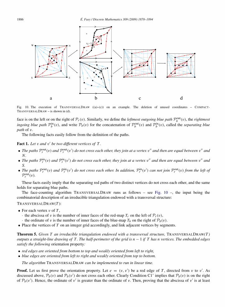
Fig. 10. The execution of TRANSVERSALDRAW ((a)–(c)) on an example. The deletion of unused coordinates – COMPACT-TRANSVERSALDRAW – is shown in (d).

face is on the left or on the right of Pr (v). Similarly, we define the leftmost outgoing blue path P outb (v), the rightmost

ingoing blue path P inb (v), and write Pb(v) for the concatenation of P out

b (v) and P inb (v), called the separating blue

path of v.The following facts easily follow from the definition of the paths.

Fact 1. Let v and v′ be two different vertices of T .

• The paths P outr (v) and P out

r (v′) do not cross each other, they join at a vertex v′′ and then are equal between v′′ andN.• The paths P in

r (v) and P inr (v′) do not cross each other, they join at a vertex v′′ and then are equal between v′′ and

S.• The paths P out

r (v) and P inr (v′) do not cross each other. In addition, P in

r (v′) can not join P out

r (v) from the left ofP out

r (v).

These facts easily imply that the separating red paths of two distinct vertices do not cross each other, and the sameholds for separating blue paths.

The face-counting algorithm TRANSVERSALDRAW runs as follows – see Fig. 10 –, the input being thecombinatorial description of an irreducible triangulation endowed with a transversal structure:

TRANSVERSALDRAW(T ):

• For each vertex v of T ,· the abscissa of v is the number of inner faces of the red-map Tr on the left of Pr (v),· the ordinate of v is the number of inner faces of the blue-map Tb on the right of Pb(v).• Place the vertices of T on an integer grid accordingly, and link adjacent vertices by segments.

Theorem 5. Given T an irreducible triangulation endowed with a transversal structure, TRANSVERSALDRAW(T )outputs a straight-line drawing of T . The half-perimeter of the grid is n − 1 if T has n vertices. The embedded edgessatisfy the following orientation property:

• red edges are oriented from bottom to top and weakly oriented from left to right,• blue edges are oriented from left to right and weakly oriented from top to bottom.

The algorithm TRANSVERSALDRAW can be implemented to run in linear time.

Proof. Let us first prove the orientation property. Let e = (v, v′) be a red edge of T , directed from v to v′. Asdiscussed above, Pb(v) and Pb(v

′) do not cross each other. Clearly Condition C1’ implies that Pb(v) is on the rightof Pb(v

′). Hence, the ordinate of v′ is greater than the ordinate of v. Then, proving that the abscissa of v′ is at least


Fig. 11. The direction properties of the edges ensure that the drawing is planar, step after step.

as large as the abscissa of v reduces to proving that Pr (v) is not on the right of Pr (v′). This follows from two easy

observations: P outr (v) is (weakly) on the left of P out

r (v′); and P inr (v′) is (weakly) on the right of P in

r (v′). Similarly, the

blue edges are oriented from left to right and weakly oriented from top to bottom.The proof that the embedding is a straight-line drawing relies on the orientation property and on the fact that the

red and the blue edges are combinatorially transversal. To carry out the proof, we use a sweeping process akin to theiterative algorithm used to find the preimage of an α0-orientation in Section 3.2. The idea consists in maintaining anoriented blue path P from W to E called the sweeping path, such that the following invariant is maintained, (Idraw):“the embedding of the edges of T that are not topologically on the right of P is a straight-line drawing delimited to thetop by the embedding of (W, N ), to the right by the embedding of (N , E), and to the bottom left by the embeddingof P ”. The sweeping path is initially (W, N , E) and then “moves” toward S. At each step, an inner face f of theblue-map of T is chosen, such that the left lateral path of f is included in P . Then, P is updated by replacing the leftlateral path of f by the right lateral path of f . Thus P remains an oriented path from W to E and is moved toward thebottom left corner of the embedding, i.e., the vertex S. The fact that the invariants are maintained is easily checkedfrom the orientation property and the fact that all the red edges inside f connect transversally the two lateral bluepaths; see Fig. 11. At the end, the sweeping path is equal to (W, S, E), so that the invariant (Idraw) exactly impliesthat the embedding of T is planar.

We show now that the half-perimeter of the grid is equal to n − 1 if T has n vertices. By definition ofTRANSVERSALDRAW, the minimal abscissa is 0 and the maximal abscissa is equal to the number of inner faces fr ofthe red-map. Similarly, the minimal ordinate is 0 and the maximal ordinate is equal to the number of inner faces fb ofthe blue-map. Hence, the half-perimeter is equal to fr + fb. We write respectively er and eb for the number of edgesof Tr and Tb. Euler’s relation ensures that the total number e of edges of T is 3n−7. Hence, eb+er = e+4 = 3n−3.In addition, Euler’s relation, applied respectively to Tr and Tb, ensures that n + fr = er + 1 and n + fb = eb + 1.Thus, fr + fb = er + eb − 2n + 2 = n − 1.

Finally, a linear implementation is obtained by suitably performing the face-counting operations. For each innervertex v of T , consider the rightmost outgoing red path, the leftmost outgoing red path, the leftmost ingoing red path,and the rightmost ingoing red path. These four paths P1, P2, P3, P4 partition the set of inner faces of the red-mapTr into four areas U(v), L(v), D(v), and S(v), that are respectively enclosed by (P1, P2), (P2, P3), (P3, P4), and(P4, P1). Let U (v), L(v), D(v) and S(v) be the numbers of inner faces of Tr in each of the four areas. The quantitiesU (v) are easily computed in one pass, by doing a traversal of the vertices of T from S to N . Similarly, the quantitiesD(v) are computed in one pass doing a traversal from N to S. Then, the quantities L(v) are computed in one pass(using D(v) and U (v)) by doing a traversal from W to E . Finally, the abscissas of all vertices can be computed usingAbs(v) = D(v)+ L(v). �

5.2. Compaction step by coordinate-deletions

Consider an irreducible triangulation T endowed with a transversal structure and embedded using the face-countingalgorithm TRANSVERSALDRAW. As observed in Fig. 10(c), some coordinate-lines might be unoccupied. Hence, anatural further step is to delete the unused coordinates, yielding a more compact drawing, as illustrated in Fig. 10(d).The corresponding algorithm is called COMPACTTRANSVERSALDRAW.

Theorem 6. Given T an irreducible triangulation endowed with a transversal structure, COMPACTTRANSVERSAL-DRAW(T ) outputs a straight-line drawing of T . The half-perimeter of the grid is at most n − 1 if T has n vertices.The embedded edges satisfy the same orientation property as TRANSVERSALDRAW(T ), and the algorithm can beimplemented to run in linear time.


Fig. 12. A random triangulation with 200 vertices embedded with the algorithms DRAW and COMPACTDRAW.

Proof. Clearly, the orientation property of the red and of the blue edges remains satisfied after coordinate-deletions.Notice that the planarity of TRANSVERSALDRAW has been proved using only the orientation property, so that thesame proof of planarity works as well for COMPACTTRANSVERSALDRAW. The linear complexity follows from theeasy property that coordinate-deletions can be performed in linear time. �

5.3. Drawing with the minimal transversal structure

Notice that, in the definition of both TRANSVERSALDRAW and COMPACTTRANSVERSALDRAW, the irreducibletriangulation is already equipped with a transversal structure. A complete straight-line drawing algorithm forirreducible triangulations is thus obtained by computing a transversal structure first, and then launching the face-counting algorithm TRANSVERSALDRAW, possibly followed by the additional step of deletion of unused coordinates(COMPACTTRANSVERSALDRAW). A natural choice for the transversal structure computed is to take the minimal onefor the distributive lattice, with the further advantage of making it possible to perform an average-case analysis of thegrid size, as we will see in Section 6. The minimal transversal structure can be computed in linear time: (1) computea transversal structure in linear time using an algorithm by Kant and He [20], (2) make the transversal structureminimal by iterated circuit reversals on the associated α0-orientations of the angular graph (the fact that the overallcomplexity of circuit reversions is linear easily follows from ideas presented in [21]). Alternatively, a linear algorithmCOMPUTEMINIMAL computing directly the minimal transversal structure is described in the PhD of the author [16].We define the following straight-line drawing algorithms for irreducible triangulations.DRAW(T ): COMPACTDRAW(T ):• Call COMPUTEMINIMAL(T ) • Call COMPUTEMINIMAL(T )• Call TRANSVERSALDRAW(T ) • Call COMPACTTRANSVERSALDRAW(T )

Simulations on random irreducible triangulations of large size (n ≈ 50000) indicate that the grid size is alwaysapproximately n

2 ×n2 with DRAW and n

2 (1−α)×n2 (1−α) with COMPACTTRANSVERSALDRAW, for some constant

α ≈ 0.18; see Fig. 12 for an example. It turns out that the size of the grid can be analyzed thanks to the closuremapping presented in Section 4. In the same way, as described by Bonichon et al. [5], the bijection of [24] makes itpossible to perform a probabilistic analysis of the grid size for straight-line drawing algorithms based on Schnyderwoods [4]. Finally let us mention that a more general procedure of compaction is described in the PhD of the author:(1) delete a set E = Er ∪ Eb of red and of blue edges such that the red orientation and the blue orientation remainbipolar, (2) call the face-counting algorithm TRANSVERSALDRAW, (3) re-insert the edges that have been deleted. Itcan be checked that the drawing thus obtained is planar and has semi-perimeter n− 1− |E |. (However the orientationproperties might not be satisfied.)

6. Analysis of the grid size of the drawing algorithms

In this section, we explain how the closure mapping gives rise to a precise probabilistic analysis of the grid size ofthe algorithms DRAW and COMPACTDRAW. The main result is as follows.


Theorem 7. Let T be a rooted irreducible triangulation with n inner vertices taken uniformly at random. Let W × Hbe the grid size of DRAW(T ) and let Wc × Hc be the grid size of COMPACTDRAW(T ). Then, the following resultshold asymptotically with high probability, up to fluctuations of order

√n,

W × H 'n

2×

n

2, Wc × Hc '

1127

n ×1127

n.

Let us mention that the concentration property also holds in a so-called ε-formulation: “for any ε > 0, theprobability that W or H are outside of [(1/2 − ε)n, (1/2 + ε)n] and the probability that Wc or Hc are outside of[(11/27− ε)n, (11/27+ ε)n] are asymptotically exponentially small”.

We first deal with the analysis of W and H , i.e., the width and the height of DRAW(T ). This task is rather easyand allows us to introduce some tools that will also be used to analyze the grid size of COMPACTDRAW(T ), namelygenerating functions and the so-called quasi-power theorem. In the sequel, the set of rooted irreducible triangulationswith n inner vertices is denoted by T ′n .

6.1. Analysis of the grid size of DRAW(T )

Given T ∈ T ′n endowed with its minimal transversal pair of bipolar orientations, the width of the grid of DRAW(T )is, by definition, the number of inner faces of the red-map Tr . Let er and fr be the numbers of inner edges and of innerfaces of Tr . Euler’s relation applied to Tr ensures that er = n+ fr − 1. By definition of the opening, er is equal to thenumber of red edges (including the stems) of the edge-bicolored ternary tree obtained by doing the opening of T . Aneasy adaptation of the proof of Theorem 4 ensures that the uniform distribution on T ′n is mapped by the opening tothe uniform distribution on rooted edge-bicolored ternary tree with n nodes. These observations lead to the followingstatement:

Fact 2. The distribution of the width of DRAW(T ) for T uniformly sampled in T ′n is equal to the distribution ofer − n − 1, where er is the number of red edges of a uniformly sampled rooted edge-bicolored ternary tree with nnodes.

We denote by R (resp. B) the set of rooted edge-bicolored ternary trees whose root leaf is incident to a red stem(resp. blue stem). For a rooted edge-bicolored ternary tree γ , we denote by |γ | the number of nodes of γ and by ξ(γ )the number of red edges of γ . We define the generating functions

R(z, u) =∑γ∈R

z|γ |uξ(γ ), B(z, u) =∑γ∈B

z|γ |uξ(γ )

that count the set R and the set B with respect to the number of nodes and the number of red edges. The generatingfunction E(z, u) counting rooted edge-bicolored ternary trees with respect to the number of nodes and the number ofred edges is thus equal to R(z, u)+ B(z, u). The classical decomposition of a rooted ternary tree at the root node intothree subtrees translates to the following equation system:{

R(z, u) = zu (1+ B(z, u)) (u + R(z, u)) (1+ B(z, u)) ,B(z, u) = z (u + R(z, u)) (1+ B(z, u)) (u + R(z, u)) .

This system is polynomial in R, B, z and u, so that one derives, by algebraic elimination, a trivariate polynomialP(E, z, u) that satisfies P(E(z, u), z, u) = 0, i.e., E(z, u) is an algebraic series.

We state now an adaptation of the quasi-power theorem [14, Thm. IX.7, Cor. IX.1], [11] for algebraic series. Thistheorem makes it possible to analyze the distribution of the number of red edges in a rooted edge-bicolored ternarytree.

Theorem 8 (Algebraic Quasi-Power Theorem). Let E(z, u) be the generating function of a combinatorial classE , where the variable z marks the size |γ | of an object γ ∈ E and the variable u marks a parameter ξ ,i.e., E(z, u) =

∑γ∈E z|γ |uξ(γ ). Assume that E(z, u) is an algebraic series, i.e., there exists a trivariate polynomial

P(E, z, u) with rational coefficients such that P(E(z, u), z, u) = 0. Consider the polynomial system:

(S) :={

P(E, z, u) = 0,∂P

∂E(E, z, u) = 0

}.


Assume that (S) has a solution {τ, ρ} at u = 1 such that τ and ρ are positive real values and thereexists no other complex solution (E, z) of (S) at u = 1 such that |z| ≤ ρ. Assume further thatthe derivative-condition { ∂

2 P∂E2 (τ, ρ, 1) 6= 0, ∂P

∂z (τ, ρ, 1) 6= 0} is satisfied. Assume also that the Jacobian of (S) withrespect to E and z does not vanish at (τ, ρ, 1), i.e.,

det

∂P

∂E(τ, ρ, 1)

∂2 P

∂E2 (τ, ρ, 1)

∂P

∂z(τ, ρ, 1)

∂2 P

∂z∂E(τ, ρ, 1)

6= 0.

Then there exists a unique pair of algebraic series (τ (u), ρ(u)) such that{P(τ (u), ρ(u), u) = 0,

∂P

∂E(τ (u), ρ(u), u) = 0, τ (1) = τ, ρ(1) = ρ

}.

Finally, assume that ρ(u) satisfies the mean condition ρ′(1) 6= 0 and variance condition ρ′′(1)ρ(1) + ρ′(1)ρ(1) −ρ′(1)2 6= 0. Then, for γ taken uniformly at random in the set of objects of E of size n, the random variable Xn = ξ(γ )

is asymptotically equal to µn, up to Gaussian fluctuations of order σ√

n, where

µ = −ρ′(1)ρ(1)

, σ 2= −

ρ′′(1)ρ(1)

−ρ′(1)ρ(1)

+

(ρ′(1)ρ(1)

)2

.

In other words, (Xn − µn)/(σ√

n) converges to the normal law.

This theorem, despite a rather long statement and several conditions to check, is easy to apply in practice. In our case,E(z, 1) is clearly equal to 2A(z) with A(z) = z(1 + A(z))3 the generating function of rooted ternary trees. Hence,at u = 1, we have P(E, z) = E/2 − z(1 + E/2)3. Using a computer algebra software, the solution of (S) at u = 1is found to be {τ = 1, ρ = 4/27}. The derivative condition and the Jacobian condition are then easily checked. Thealgebraic function ρ(u) is obtained by taking the resultant of the two equations of (S) with respect to E ; then thefactor Q(z, u) of the resultant such that Q(ρ, 1) = 0 gives an algebraic equation for ρ(u), i.e., Q(ρ(u), u) = 0.From the algebraic equation Q(ρ(u), u) = 0, the derivative and second derivative of ρ(u) at u = 1 are readilycalculated. To calculate ρ′(1), we derive Q(ρ(u), u) = 0 and find ∂Q

∂z (ρ(u), u)ρ′(u) + ∂Q∂u (ρ(u), u) = 0, so that

ρ′(1) = − ∂Q∂u (ρ, τ )/

∂Q∂z (ρ, τ ). The mean condition and variance condition are readily checked and we find µ = 3/2.

Hence, the number er of red edges in a random rooted edge-bicolored ternary tree is asymptotically equal to 3n/2, upto fluctuations of order

√n. This result, together with Fact 2, ensure that the width of DRAW(T ), for T taken uniformly

at random in T ′n , is asymptotically equal to n/2 up to fluctuations of order√

n. The result is the same for the height Hof DRAW(T ), by stability of T ′n and of the algorithm DRAW under the π/2 clockwise rotation. Thus, we have provedthe statement of Theorem 7 on the distribution of the grid size of DRAW(T ).

6.2. Analysis of the grid size of COMPACTDRAW(T )

6.2.1. Overview of the proofNow we concentrate on the distribution of the grid width of COMPACTDRAW(T ), for T taken uniformly at random

in T ′n (the analysis of the grid height is similar). By definition, the width of COMPACTDRAW(T ) is W−∆abs(T ), whereW is the width of DRAW(T ) and ∆abs is the number of abscissas not used by DRAW(T ). We have already proved thatW is asymptotically equal to n/2 up to fluctuations of order

√n. Hence, to obtain the statement of Theorem 7 about

Wc, it is sufficient to prove that ∆abs(T ) is asymptotically equal to 5n/54 up to fluctuations of order√

n. The steps ofthe proof are the following: first, the abscissas that are not used by DRAW(T ) are associated with specific edges of T ;then these edges of T are shown to correspond to specific red edges of the ternary tree obtained by doing the openingof T . Finally, using generating functions and the algebraic quasi-power theorem, it is proved that the number of suchedges in a random rooted edge-bicolored ternary tree with n nodes is asymptotically equal to 5n/54, up to fluctuationsof order

√n.

6.2.2. Characterization of unused abscissas as particular edges of TWe analyze the number of unused abscissas of DRAW(T ), i.e., the number of vertical lines of the grid that bear no

vertex of T . Recall that the width of the grid of DRAW(T ) is the number of inner faces fr of the red-map Tr of T ,


where Tr is obtained by computing the minimal transversal pair of bipolar orientations of T and then removing all blueedges. By definition of TRANSVERSALDRAW(T ), the abscissa Abs(v) of a vertex v of T is obtained by associatingwith v an oriented path Pr (v) of the red-map, called the separating red path of v (as defined in Section 5), and thencounting the number of inner faces of Tr on the left of Pr (v). We show first that each abscissa-candidate 1 ≤ i ≤ frcan be associated with a unique inner face of Tr – for which we write Abs( f ) = i – such that the existence of a vertexv of T with Abs(v) = i only depends on the configuration of the edge at the bottom right corner of f .

Let us start with a few definitions. Given e = (v, v′) an edge of Tr directed from v to v′, the separating red pathof e, denoted by Pr (e), is the path obtained by concatenating the leftmost outgoing red path of v′, the edge e, andthe rightmost ingoing red path of v. We recall that, for each inner face f of Tr , there are two vertices s f and t f of fsuch that the boundary of f consists of a left and a right lateral paths going from s f to t f . The separating red path off , denoted by Pr ( f ), is defined as the concatenation of the leftmost outgoing red path of t f , of the right lateral pathPright( f ) of f , and of the rightmost ingoing red path of s f . Observe that the first edge e f of Pright( f ), called bottomright edge of f , satisfies Pr ( f ) = Pr (e f ).

Lemma 11. Let e and e′ be two different edges of the red-map Tr . Then the separating paths Pr (e) and Pr (e′) do notcross each other.

Proof. First it is easily checked that the bipolar orientation on red edges (and similarly the one on blue edges) hasno transitive edge; otherwise, there would be a face of the red-map with one lateral path reduced to an edge, incontradiction with the presence of transversal blue edges within the face. Hence only three cases can arise: either e′

and Pr (e) do not intersect, or they intersect at a unique extremity of e′, or e′ is on Pr (e). Fact 1 allows us to checkthat Pr (e) and Pr (e′) do not cross each other for each of the three cases. �

Recall that the separating red path of a face f is the separating red path of its bottom right edge. Thus, Lemma 11ensures that the separating red paths Pr ( f ) and Pr ( f ′) of two different inner faces f and f ′ of Tr do not cross eachother. In addition, it is easy to see that they are different using the fact that the bottom right edge of a face is not theleftmost outgoing red edge at its origin. As a consequence, Abs( f ) 6= Abs( f ′). There are fr inner faces in Tr , eachinner face f clearly satisfying 1 ≤ Abs( f ) ≤ fr . Hence the pigeonhole principle yields:

Fact 3. For 1 ≤ i ≤ fr , there exists a unique inner face f of T such that Abs( f ) = i .

Thus, the inner faces of Tr are strictly ordered from left to right according to their associated abscissa.

Lemma 12. The separating red paths of an edge e of the red-map Tr and of a vertex v ∈ T do not cross each other.In addition, given e an edge of Tr , there exists a vertex v such that Pr (v) = Pr (e) iff either e is the rightmost ingoingred edge at its end-vertex or e is the leftmost outgoing red edge at its origin.

Proof. The fact that Pr (e) and Pr (v) do not cross each other is easily checked using Fact 1. The second statementof the lemma follows from a few observations. Denote by v1 the origin of e and by v2 the end-vertex of e. If v isnot on Pr (e) then clearly Pr (v) is not equal to Pr (e). If v is on Pr (e) between v2 and N , then Pr (v) = Pr (e) iffall edges of Pr (e) between v1 and v are the rightmost ingoing red edge at their end-vertex. If v is on Pr (e) betweenS and v1, then Pr (v) = Pr (e) iff all edges of Pr (e) between v and v2 are the leftmost outgoing red edge at theirorigin. It follows from these observations that Pr (v2) = Pr (e) if e is the rightmost ingoing red edge at its end-vertex,that Pr (v1) = Pr (e) if e is the leftmost outgoing red edge at its origin, and that no vertex v satisfies Pr (v) = Pr (e)otherwise. �

Definition. Given an irreducible triangulation T endowed with its minimal transversal edge-partition, a ccw-internaledge of T is an inner edge e of T such that the counterclockwise-consecutive edge at each extremity of e has the samecolor as e. Hence, on the minimal transversal pair of bipolar orientations, a ccw-internal red edge is an inner red edgeof T that is neither the leftmost outgoing red edge at its origin nor the rightmost ingoing red edge at its end-vertex.

Lemma 13. The number of abscissas not used by DRAW(T ) is equal to the number of ccw-internal red edges of T .Similarly, the number of ordinates not used by DRAW(T ) is equal to the number of ccw-internal blue edges of T .


Proof. Let 1 ≤ i ≤ fr be an abscissa-candidate and let f be the unique inner face of Tr such that Abs( f ) = i . Recallthat the separating red path Pr ( f ) is equal to the separating red path of the bottom right edge e f of f . Lemma 12ensures that i is not the abscissa of any vertex of T iff e f is a ccw-internal red edge of T . Hence, the number ofabscissas not used by DRAW(T ) is equal to the number of ccw-internal red edges of T that are the bottom right edgeof an inner face of Tr . This quantity is also the number of ccw-internal red edges of T . Indeed, a ccw-internal red edgee is the bottom right edge of the inner face of Tr on its left, as e is not the leftmost outgoing red edge at its origin. �

6.2.3. Reduction to the analysis of a parameter on ternary treesAccording to Lemma 13, the number of coordinate-lines that bear no vertex in DRAW(T ) is equal to the number of

ccw-internal edges of T . As we show next, the ccw-internal edges of T correspond to particular edges of the ternarytree A obtained by doing the opening of T . We define an internal edge of a ternary tree A as a closed edge e of A suchthat both edges following e in clockwise order around each extremity of e are closed edges.

Lemma 14. Let T be an irreducible triangulation and let A be the ternary tree obtained by doing the opening of T , Tbeing endowed with its minimal transversal edge-partition and A being endowed with the induced edge-bicoloration.Then each ccw-internal red (blue) edge of T corresponds, via the opening of T , to an internal red (blue) edge of A.

Proof. Let e = (v, v′) be a ccw-internal red edge of T . By definition, the ccw-consecutive edge of e at v′ is red. Hencethe cw-consecutive edge of e at v is blue (otherwise there would be a unicolored face in T , contradicting Lemma 1).Similarly, the cw-consecutive edge of e at v′ is blue. Hence, by definition of the opening mapping, e is a closed edgeof A. To prove that e is an internal edge of A, we have to prove that the cw-consecutive edge of A at each extremityof e is a closed edge of A. Let e1, . . . , ek be the clockwise interval of blue edges of T following e in clockwise orderaround v (the word interval referring to the terminology of Condition C1); and let v1, . . . , vk be the correspondingsequence of neighbours of v. By definition of the opening mapping, the edge of A following e in clockwise orderaround v is ek . To prove that ek is a closed edge of A it remains to show that the edge e′ ∈ T following ek in clockwiseorder around vk is red. If k = 1, e′ is also the edge following e in counterclockwise order around v′. Hence, the factthat e is internal red ensures that e′ is red. If k ≥ 2, then e′ = (vk, vk−1). As (v, vk) and (v, vk−1) are blue, Lemma 1ensures that (vk, vk−1) is red. Hence, ek is a closed edge of A. Similarly, the edge of A following e in clockwise orderaround v′ is a closed edge of A. Thus, e is an internal edge of A.

Conversely, let e = (v, v′) be an internal red edge of A. By definition of the opening mapping, the edge ev ∈ Tfollowing e in ccw order around v has the same color as e iff the half-edge of ev incident to v has been created duringa local closure. The same holds with the edge ev′ following e in ccw order around v′. We claim that this conditionis satisfied by e at v′ (and similarly at v). Indeed, the sides of closed edges incident to the outer face of the figure Fobtained as the partial closure of A are such that the cw-consecutive edge at their right extremity (looking toward theouter face) is a stem. Hence, e is not incident to the outer face of F , so that there exists a local closure whose effectis to close a triangular face incident to the right side of e (traversed from v to v′). The stem s involved in this localclosure can not be incident to v, as the edge of A following e in cw order around v is not a stem. Hence e = (v, v′) isthe second closed edge following the stem, so that the newly created half-edge (opposite to s) is incident to v′. Thisconcludes the proof. �

Lemma 14 yields the following result that, as Fact 3, follows from an easy adaptation of the proof of Theorem 4.

Fact 4. The distribution of the parameter ∆abs(T ), for T taken uniformly at random in T ′n , is equal to the distributionof the number of internal red edges in a rooted edge-bicolored ternary tree with n nodes taken uniformly at random.

Let Xn be the random variable denoting the number of internal red edges of a rooted edge-bicolored ternary tree withn nodes taken uniformly at random. Fact 4 and the discussion in the overview ensure that the statement of Theorem 7about Wc is proved by analyzing the distribution of Xn and showing a concentration around 5n/54.

6.2.4. Analysis of the random variable Xn

We introduce the generating functions F(z, u) and G(z, u) counting respectively red-rooted ternary trees and blue-rooted ternary trees with respect to the number of nodes and the number of internal red edges. As for the seriesR(z, u) and B(z, u) involved in the analysis of DRAW, an equation system linking the series F(z, u) and G(z, u) canbe obtained by decomposing a rooted ternary tree at its root node into three subtrees.


Fig. 13. Decomposition at the root node keeping track of the number of internal red edges.

To keep track of the parameter counting internal red edges, we introduce two auxiliary generating functions: F(z, u)is the series counting red-rooted ternary trees with respect to the number of nodes and the number of internal red edges,with the difference that the root red stem is also considered as an internal red edge if its right child-edge is a closededge; and G(z, u) is the series counting blue-rooted ternary trees with respect to the number of nodes and the numberof internal red edges, with the difference that the left child-edge e of the root node is also considered as an internal rededge if e is a closed edge and if the right child-edge of e is a closed edge. The decomposition at the root node keepingtrack of the number of internal red edges is shown in Fig. 13. This directly translates to the following system:

F(z, u) = z(1+ F)+ zu(1+ F)G + z(1+ F)G + zuG(1+ F)GG(z, u) = z(1+ F)(1+ F)+ z(1+ F)G(1+ F)F(z, u) = z(1+ F)(1+ G)+ zG(1+ F)(1+ G)G(z, u) = z(1+ F)2 + z(1+ F)G(1+ F)

(3)

Let H(z, u) be the series counting rooted edge-bicolored ternary trees by the numbers of nodes and internal rededges; clearly H(z, u) = F(z, u)+G(z, u). An algebraic equation P(H(z, u), z, u) = 0 is easily computed from (3).Then, the algebraic quasi-power theorem can be applied to the algebraic generating function H(z, u). All conditionsare easily checked and the algebraic series ρ(u) which we obtain satisfies µ = −ρ′(1)/ρ(1) = 5/54. This yieldsthe statement of Theorem 7 on the distribution of Wc. The result is the same for Hc, because the distribution of Hcis equal to the distribution of Wc, by stability of T ′n and of COMPACTDRAW under the π/2 clockwise rotation. Thisconcludes the proof of Theorem 7.

7. Conclusion

Several families of planar maps are characterized by the existence of a specific combinatorial structure for each mapof the family (bipolar orientations for 2-connected maps, Schnyder woods for triangulations). This article providesa detailed study of so-called transversal structures, which are specific to the family of triangulations of the 4-gonwith no filled 3-cycle — called irreducible triangulations. The two main results that we obtain related to transversalstructures are a bijection between irreducible triangulations and ternary trees, as well as a new straight-line drawingalgorithm for irreducible triangulations. The bijection allows us to count irreducible triangulations and the closelyrelated family of 4-connected triangulations.

Surprisingly, the bijection – combined with some modern tools of analytic combinatorics – also makes it possibleto analyze the grid size of the straight-line drawing; for a random irreducible triangulation with n vertices, the gridsize is with high probability 11n/27 × 11n/27 up to an additive error O(

√n). In comparison, the best previously

known algorithm [22] only guarantees a grid size (dn/2e − 1) × bn/2c. The principle of our straight-line drawingalgorithm has also been recently applied to the family of quadrangulations [15,16]; for a random quadrangulation with


n vertices, the grid size is with high probability 13n/27× 13n/27 up to an additive error O(√

n), which improves onthe grid size (dn/2e − 1)× bn/2c guaranteed by [2].

Acknowledgments

I would like to thank my advisor Gilles Schaeffer, who has greatly helped me to produce this work throughnumerous discussions, steady encouragement and useful suggestions. I also thank Nicolas Bonichon, Luca CastelliAleardi, and Philippe Flajolet for fruitful discussions, Roberto Tamassia for having pointed reference [1] out to me,and Thomas Pillot for very efficient implementations of all algorithms presented in this article. Finally, I am verygrateful to the two anonymous referees for their detailed corrections and insightful remarks.

References

[1] G. Di Battista, R. Tamassia, I.G. Tollis, Area requirement and symmetry display of planar upward drawings, Discrete Comput. Geom. 7 (1992)381–401.

[2] T. Biedl, F.J. Brandenburg, Drawing planar bipartite graphs with small area, in: Proceedings of CCCG, Windsor, 2005.[3] T.C. Biedl, G. Kant, M. Kaufmann, On triangulating planar graphs under the four-connectivity constraint, Algorithmica 19 (4) (1997) 427–446.[4] N. Bonichon, S. Felsner, M. Mosbah, Convex drawings of 3-connected plane graphs, in: GD’04: Proceedings of the Symposium on Graph

Drawing, Springer-Verlag, 2004, pp. 287–299.[5] N. Bonichon, C. Gavoille, N. Hanusse, D. Poulalhon, G. Schaeffer, Planar graphs, via well-orderly maps and trees, in: 30th International

Workshop, Graph – Theoretic Concepts in Computer Science (WG), in: Lecture Notes in Computer Science, vol. 3353, Springer-Verlag,2004, pp. 270–284.

[6] E. Brehm, 3-orientations and Schnyder 3-tree-decompositions, Master’s Thesis, FB Mathematik und Informatik, Freie Universitat Berlin,2000.

[7] W.G. Brown, Enumeration of triangulations of the disk, in: Proceedings of the London Mathematical Society, 1964, pp. 746–768.[8] M. de Berg, E. Mumford, B. Speckmann, On rectilinear duals for vertex-weighted plane graphs, in: GD’05: Proceedings of the Symposium

on Graph Drawing, Springer-Verlag, 2006.[9] H. de Fraysseix, P. Ossona de Mendez, J. Pach, Representation of planar graphs by segments, Intuitive Geom. 63 (1991) 109–117.

[10] H. De Fraysseix, P. Ossona de Mendez, P. Rosenstiehl, Bipolar orientations revisited, Discrete Appl. Math. 56 (2–3) (1995) 157–179.[11] M. Drmota, Systems of functional equations, Random Structures Algorithms 10 (1–2) (1997) 103–124.[12] S. Felsner, Convex drawings of planar graphs and the order dimension of 3-polytopes, Order 18 (2001) 19–37.[13] S. Felsner, Lattice structures from planar graphs, Electron. J. Combin. R15 (2004) 24p.[14] P. Flajolet, R. Sedgewick, Analytic Combinatorics. Available at http://algo.inria.fr/flajolet/Publications/book051001.pdf. Preliminary version

of the forthcoming book.[15] E. Fusy, Straight-line drawing of quadrangulations, in: Proceedings of Graph Drawing’06, Karlsruhe, Springer, 2006, pp. 234–239.[16] E. Fusy, Combinatoire des cartes planaires et applications algorithmiques, Ph.D. Thesis, Ecole Polytechnique, 2007.[17] E. Fusy, D. Poulalhon, G. Schaeffer, Dissections and trees, with applications to optimal mesh encoding and to random sampling, in: 16th

Annual ACM-SIAM Symposium on Discrete Algorithms, January 2005.[18] X. He, On finding the rectangular duals of planar triangulated graphs, SIAM J. Comput. 22 (1993) 1218–1226.[19] X. He, Grid embedding of 4-connected plane graphs, Discrete Comput. Geom. (1997) 339–358.[20] G. Kant, Xin He, Regular edge labeling of 4-connected plane graphs and its applications in graph drawing problems, Theoret. Comput. Sci.

172 (1–2) (1997) 175–193.[21] S. Khuller, J. Naor, P.N. Klein, The lattice structure of flow in planar graphs, SIAM J. Discrete Math. 6 (3) (1993) 477–490.[22] K. Miura, S. Nakano, T. Nishizeki, Grid drawings of four-connected plane graphs, Discrete Comput. Geom. 26 (2) (2001) 73–87.[23] P. Ossona de Mendez, Orientations bipolaires, Ph.D. Thesis, Paris, 1994.[24] D. Poulalhon, G. Schaeffer, Optimal coding and sampling of triangulations, in: Automata, Languages and Programming. 30th International

Colloquium, ICALP 2003, vol. 2719, Eindhoven, 2003, pp. 1080–1094.[25] G. Schaeffer, Conjugaison d’arbres et cartes combinatoires aleatoires, Ph.D. Thesis, Universite Bordeaux I, 1998.[26] G. Schaeffer, Random sampling of large planar maps and convex polyhedra, in: Annual ACM Symposium on Theory of Computing (Atlanta,

GA, 1999), ACM, New York, 1999, pp. 760–769 (electronic).[27] W. Schnyder, Planar graphs and poset dimension, Order 5 (1989) 323–343.[28] W. Schnyder, Embedding planar graphs on the grid, in: SODA’90: Proceedings of the First Annual ACM-SIAM Symposium on Discrete

Algorithms, 1990, pp. 138–148.[29] B. Speckmann, M. Van Kreveld, On rectangular cartograms, Technical report, 2004.[30] W.T. Tutte, A census of planar triangulations, Canad. J. Math. 14 (1962) 21–38.

http://algo.inria.fr/flajolet/Publications/book051001.pdf

Documents

Transversal structures on triangulations: A combinatorial study and straight-line drawings