Embed Size (px)
Citation preview
Transportations Systems Modeling and Applications in Earthquake Engineering
Report No. 10-03
Liang Chang Amr S. Elnashai Billie F. Spencer
JunHo Song Yanfeng Ouyang
July 2010
ii
ABSTRACT
Transportation networks constitute one class of major civil infrastructure systems that is a
critical backbone of modern society. Physical damage and functional loss to transportation
infrastructure systems not only hinder everyday societal and commercial activities, but also
impair post-disaster response and recovery, leading to substantial socio-economic consequences.
Therefore, understanding and modeling the disastrous impact on the transportation
infrastructures and the corresponding changes of travel patterns under extreme events are vital
for stakeholders, emergency managers, and government agencies to mitigate, prepare for,
respond to, and recover from the potential impact.
This research is aimed at developing a systematic approach for risk modeling and disaster
management of transportation systems in the context of earthquake engineering. First, by
employing the performance metrics that are suited for immediate post-disaster response, this
dissertation explores efficient methodologies to maximize the overall system functionality and
the benefit of mitigation investment for transportation infrastructure systems. Furthermore, the
regions potentially unreachable after a damaging earthquake are identified promptly by using
network reachability algorithms that provide essential information for rapid emergency response
decision-making. Lastly, an integrated simulation model of travel demand that accounts for
damage of bridge and building structures, release of hazardous materials, and influences of
emergency shelters and hospitals, is developed to approximate the “abnormal” post-earthquake
travel patterns and evaluate the functional loss of the transportation systems.
This study extends the understanding of disaster management of transportation
infrastructure systems. The methodologies developed in this study have the following
significance: (i) help leverage available mitigation resources to improve the disaster resilience

iii
and functionality of transportation infrastructure systems; (ii) enable emergency response and
recovery teams to rapidly identify and evaluate the performance of optimal routes for emergency
ingress and egress; (iii) accurately estimate traffic congestion under extreme events; and (iv)
provide important insights necessary to make decisions on protecting these systems to meet the
needs of current and future generations.

iv
ACKNOWLEDGMENTS
This work could not have been completed without the members of my doctoral committee.
First, I wish to express my sincere gratitude to my advisors, Professor Amr S. Elnashai and
Professor Billie F. Spencer Jr. for their continuous support and encouragement. I feel privileged
and would like to thank them for providing insight in all aspects of this research and nurturing
my academic and professional development through their mentorships. I would also extend my
gratitude to my advisory committee, Professor Junho Song and Professor Yanfeng Ouyang for
taking their time to review this work and to provide advice, criticism, and recommendations.
Many other people contributed to the development of this research. Particularly, I would
like to acknowledge Dr. YoungSuk Kim of EQECat Inc., and Dr. JongSung Lee of the National
Center for Supercomputing Applications (NCSA) for their expertise and support. I sincerely
appreciate Professor Travis S. Waller of the University of Texas at Austin for his advice on
transportation modeling, and Mr. Timothy Gress for the support and help in the acquisition of
necessary transportation data. I would like to gratefully thank Professor Tschangho John Kim,
Professor Zhenghong Tang of University of Nebraska–Lincoln, and Professor Yang Zhang of
Virginia Polytechnic Institute and State University, for their valuable discussions and assistances.
I would also like to thank many who have provided valuable information and practical
insight. These people include but not limited to: Dr. Eugene Schweig (U.S. Geological Survey),
Professor Chris Cramer (University of Memphis), Professor Reginald DesRoches (Georgia
Institute of Technology), Mr. Steve Besemer (Missouri State Emergency Management Agency),
Mr. Richard Bennett (Missouri Department of Transportation), Mr. Phillip Anello (Illinois
Emergency Management Agency), Mr. Scott Clarke and Mr. Omar Abou-Samra (American Red
Cross), Mr. Jim Wild, Ms. Lubna Shoaib, and Mr. Johnnie Smith (East-West Gateway Council

v
of Governments), Mr. Richard Bowker (Memphis Light, Gas and Water Division), Mr. Greg
Duncan, Mr. Terry Leatherwood, and Mr. Wayne Seger (Tennessee Department of
Transportation), Ms. Martha Lott and Mr. Pragati Srivastava (Memphis Urban Area Metropolitan
Planning Organization).
I am grateful to my fellow students in the Mid-America Earthquake Center, to my friends at
the University of Illinois at Urbana-Champaign, and especially to Lisa Cleveland, Can Unen,
Joshua Steelman, Young Joo Lee, Wen Hee Kang, Jun Ji, Zhongzhuo Li, Sheng-Lin Lin, Oh-
Song Kwon, Fan Peng, Xiaopeng Li, and Wei Xu. Finally, I owe my tremendous thanks to my
family for their unconditional love and steady encouragement through the course of my studies.
The work was supported by the National Science Foundation under the Award Number
EEC-9701785 through the Mid-America Earthquake Center. Additional support was provided by
the Federal Emergency Management Agency through a grant from the U.S. Army Corps of
Engineers (Army W9132T-06-2).
vi
TABLE OF CONTENTS
LIST OF FIGURES .................................................................................................................VIII
LIST OF TABLES ....................................................................................................................... X
CHAPTER I INTRODUCTION .............................................................................................. 1
1.1 BACKGROUND...................................................................................................................... 1 1.2 CHALLENGES AND ISSUES .................................................................................................... 2 1.3 OBJECTIVES AND EXPECTED IMPACT OF RESEARCH............................................................. 4 1.4 SCOPE .................................................................................................................................. 6 1.5 ORGANIZATION OF DISSERTATION ....................................................................................... 6
CHAPTER II LITERATURE REVIEW.................................................................................. 8
2.1 SEISMIC RISK ASSESSMENT OF INFRASTRUCTURE COMPONENTS......................................... 8 2.1.1 Hazard Definition............................................................................................................ 9 2.1.2 Structural Vulnerability and Functionality...................................................................... 9 2.2 PERFORMANCE MODELING AND EVALUATION OF TRANSPORTATION SYSTEMS................. 14 2.2.1 Travel Delay Cost.......................................................................................................... 15 2.2.2 Network Flow Capacity ................................................................................................ 30 2.2.3 Reliability of Network Reachability ............................................................................. 31 2.3 HAZARD MITIGATION FOR TRANSPORTATION SYSTEMS .................................................... 36 2.3.1 Component-Level Approaches...................................................................................... 37 2.3.2 Network-Level Approaches .......................................................................................... 39 2.4 SUMMARY.......................................................................................................................... 42
CHAPTER III NETWORK-BASED PERFORMANCE MODELING FRAMEWORK . 45
3.1 METHODOLOGICAL FRAMEWORK ...................................................................................... 45 3.2 THE NEW MADRID FAULT ZONE AND HAZARD CHARACTERIZATION ................................ 47 3.3 BRIDGE DAMAGE ASSESSMENT ......................................................................................... 48 3.4 BRIDGE DAMAGE-FUNCTIONALITY RELATIONSHIP............................................................ 52 3.5 NETWORK ANALYSIS OF TRANSPORTATION SYSTEMS ....................................................... 53 3.5.1 Network Flow Capacity ................................................................................................ 54 3.5.2 Reliability of Network Reachability ............................................................................. 55 3.5.3 Travel Delay Cost Metric.............................................................................................. 57
CHAPTER IV OD-INDEPENDENT PERFORMANCE EVALUATION AND SEISMIC RETROFIT PROGRAM PLANNING ..................................................................................... 60
4.1 NETWORK FLOW CAPACITY-BASED NBSR........................................................................ 60 4.1.1 Mathematical Framework ............................................................................................. 61 4.1.2 Monte Carlo Sampling of Bridge Residual Capacity Scenarios ................................... 64 4.1.3 Optimization Models..................................................................................................... 67 4.1.4 Effectiveness Measurement and Project Selection........................................................ 71 4.1.5 Convergence Tests ........................................................................................................ 73 4.1.6 Sensitivity to Ground Motion Correlation .................................................................... 76 4.1.7 Numerical Case Study: the Memphis Road Network ................................................... 80
vii
4.1.8 Discussion ..................................................................................................................... 87 4.2 RELIABILITY OF NETWORK REACHABILITY........................................................................ 88 4.2.1 Recursive Decomposition Algorithm for Reachability Reliability ............................... 89 4.2.2 Numerical Example: the Sioux-Falls Road Network.................................................... 90 4.2.3 Case Study: the Memphis Road Network ..................................................................... 92 4.2.4 Results and Discussion.................................................................................................. 93 4.3 SUMMARY.......................................................................................................................... 95
CHAPTER V MODELING THE POST-EARTHQUAKE TRAVEL DEMAND.............. 97
5.1 INTRODUCTION................................................................................................................... 97 5.2 METHODOLOGY FOR TRAVEL DEMAND MODELING........................................................... 98 5.2.1 Scenarios and Major Assumptions................................................................................ 98 5.2.2 Major Modeling Steps................................................................................................. 102 5.3 CASE STUDIES.................................................................................................................. 107 5.3.1 Sioux-Falls Road Network .......................................................................................... 107 5.3.2 Transportation Network of St. Louis MPO................................................................. 117 5.4. SUMMARY....................................................................................................................... 129
CHAPTER VI CONCLUSIONS AND FUTURE RESEARCH......................................... 130
6.1 CONCLUSIONS .................................................................................................................. 130 6.2 FUTURE RESEARCH .......................................................................................................... 133
REFERENCES.......................................................................................................................... 136
APPENDIX A EFFECTIVENESS BASED ON REDUCED REPAIR COST.................. 153
APPENDIX B VERIFICATION OF THE RECURSIVE DECOMPOSITION ALGORITHM........................................................................................................................... 154
APPENDIX C MODELING UNCERTAINTY AND CORRELATION OF GROUND MOTION ................................................................................................................................... 156
C.1 SIMULATION OF SPATIALLY VARIABLE GROUND MOTIONS ............................................ 156 C.2 PROCEDURES ................................................................................................................... 157 C.3 NUMERICAL EXAMPLE .................................................................................................... 160 C.3.1 Intra-Event Uncertainty ............................................................................................. 160 C.3.2 Inter-Event Uncertainty ............................................................................................. 163 C.3.3 Consideration of both Inter- and Intra-Event Uncertainties ...................................... 164
APPENDIX D VERIFICATION OF THE DUE MODELS ............................................... 166
APPENDIX E SIOUX-FALLS NETWORK LINK DATA AND DEMAND INFORMATION....................................................................................................................... 168
viii
LIST OF FIGURES
Figure 1 Depiction of structural fragility curves .......................................................................... 10 Figure 2 Travel demands in static and dynamic traffic assignment models ................................. 18 Figure 3 Procedures of the NBSR Approach (Kim et al. 2008) ................................................... 41 Figure 4 Methodological framework of the proposed research.................................................... 46 Figure 5 NMSZ zone structure ..................................................................................................... 49 Figure 6 PGA map of a M7.7 earthquake on all three New Madrid fault segments (g)............... 50 Figure 7 Computing exceedance probabilities for damage states................................................. 52 Figure 8 Methodological framework of network flow capacity-based NBSR ............................. 64 Figure 9 Sioux-Falls network for convergence test ...................................................................... 74 Figure 10 Convergence test of Monte Carlo sampling for network flow capacity....................... 76 Figure 11 Convergence test of network flow capacity ................................................................. 76 Figure 12 NGA hazard map (M8.0) and the Sioux-Falls road network ....................................... 78 Figure 13 Road network in the Memphis metropolitan area, Tennessee...................................... 82 Figure 14 Seismic hazard map for Memphis MPO (the M7.7 NMSZ earthquake scenario) ....... 83 Figure 15 Fragility curves of multi-span simply supported (MSSS) steel bridges....................... 83 Figure 16 Spatial distribution of bridge retrofit program under $1 million budget...................... 86 Figure 17 Budget-effectiveness curves......................................................................................... 87 Figure 18 Illustration of the recursive decomposition algorithm ................................................. 90 Figure 19 Sioux-Falls network for network reachability.............................................................. 91 Figure 20 Probability of disconnection (node 1) .......................................................................... 91 Figure 21 Nodal disconnection probability .................................................................................. 92 Figure 22 Simplified Memphis road network with the subjunctive sink...................................... 93 Figure 23 Reachability reliabilities of network nodes .................................................................. 94 Figure 24 Reliability of reachability to safe zones (case II) ......................................................... 94 Figure 25 Classification of zone types........................................................................................ 101 Figure 26 Illustration of TAZ types............................................................................................ 101 Figure 27 Methodological framework for demand modeling and performance assessment ...... 102 Figure 28 Flowchart of trip generation ....................................................................................... 103 Figure 29 Structural fragility curves for the estimation of damaged buildings .......................... 105 Figure 30 Sioux-Falls road network with evacuation and safe zones......................................... 108 Figure 31 Traffic congestion (volume-capacity ratio) by the DUE model (night scenario)....... 110 Figure 32 Traffic congestion (volume-capacity ratio) by the DUE model (day scenario) ......... 111 Figure 33 Traffic congestion (volume-capacity ratio) by the DTA model (night scenario)....... 112 Figure 34 Traffic congestion (volume-capacity ratio) by the DTA model (day scenario) ......... 113 Figure 35 Total system travel time for Sioux-Falls network ...................................................... 116 Figure 36 Transportation network of St. Louis MPO................................................................. 119 Figure 37 St. Louis MPO PGA map and bridge functionality (day 0) ....................................... 119 Figure 38 Demand generation for St. Louis MPO region........................................................... 120 Figure 39 Traffic congestion of St. Louis MPO network (day scenario) ................................... 124 Figure 40 Traffic congestion of St. Louis MPO network (night scenario)................................. 125 Figure 41 Link traffic flow on major Mississippi River crossing bridges.................................. 126 Figure 42 TSTT for the St. Louis MPO road network................................................................ 128 Figure A1 Benchmark networks for network reachability analyses........................................... 154

ix
Figure A2 Plots of PSD and autocorrelation functions............................................................... 161 Figure A3 Sample functions of inter-event uncertainty (spatial correlation) ............................. 162 Figure A4 Ground motion with intra-event uncertainty (spatial correlation)............................. 163 Figure A5 Sample function of intra-event uncertainty ............................................................... 164 Figure A6 With both intra- and inter-event uncertainties........................................................... 165
x
LIST OF TABLES
Table 1 Fragility parameters for MSC steel bridge (Padgett 2007).............................................. 50 Table 2 Bridge damage-functionality relationship (Padgett and DesRoches 2007) ..................... 53 Table 3 Bridge information for convergence test ......................................................................... 74 Table 4 Post-earthquake network flow capacity........................................................................... 75 Table 5 Effects of ground motion uncertainty and correlation on system performance............... 78 Table 6 Top 20 bridges with highest effectiveness-cost ratios..................................................... 258H84 123HTable 7 Network reachability with convergence criteria of 0.001 ............................................... 259H93 124HTable 8 Characteristics of zonal traffic generation..................................................................... 260H101 125HTable 9 Link traffic flow by the DUE model (PCU/hr).............................................................. 261H114 126HTable 10 Link traffic flow by the DTA model (PCU/hr)............................................................ 262H114 127HTable 11 Cross-sectional egress and ingress travel flow by the DUE model (PCU/hr) ............. 263H115 128HTable 12 Cross-sectional egress and ingress travel flow by the DTA model (PCU/hr) ............. 264H115 129HTable 13 St. Louis MPO major river crossing bridges ............................................................... 265H126 130HTable 14 Cross-Mississippi River traffic flow............................................................................ 266H128 131HTable A1 System connectivity reliability verification for benchmark networks........................ 267H155 132HTable A2 Verification of DUE models ....................................................................................... 268H167 133HTable A3 Link property of the Sioux-Falls network................................................................... 269H168 134HTable A4 Origin-destination matrix for Sioux-Falls network (night scenario) .......................... 270H170 135HTable A5 Origin-destination matrix for Sioux-Falls network (day scenario)............................. 271H170
1
CHAPTER I INTRODUCTION
1.1 Background
Transportation systems, together with energy, water, and telecommunication networks are
the major civil infrastructure systems providing critical backbones of modern societies (Duke
1981). Transportation systems also serve as escape routes for survivors of disasters and provide
an emergency transport network for rescue workers, construction repair teams, and disaster relief
(Earthquake Engineering Research Institute [EERI] 1986). These infrastructure systems are not
only continuously deteriorating over the course of service, but also particularly vulnerable to
seismic hazards. For example, more than 26% of the bridges in the U.S. are either structurally
deficient or functionally obsolete, requiring a $17 billion annual investment to substantially
improve their deteriorating conditions (American Society of Civil Engineers [ASCE] 2009).
The physical damage and functionality loss of the transportation infrastructure systems not
only hinder societal and commercial activities, but also impair post-disaster response and
recovery (Chang and Nojima 1998; Basőz and Kiremidjian 1996; Nojima 1998), resulting in
substantial socio-economic losses (Eguchi et al. 1998; Scawthorn et al. 1997; National Research
Council [NRC] 1999). Transportation networks with collapsed bridges could result in severe
system functionality loss and hamper post-disaster emergency response. For example, emergency
rescuers will not be able to get access to the impacted area if transportation infrastructures
collapse due to earthquake or landslide, as evidenced by the recent devastating earthquakes. It is
crucial that transportation networks retain their traffic carrying capacities after a disastrous
earthquake, so that the population at risk can evacuate efficiently to safe zones and emergency
relief resource be dispatched to the impacted area timely.
2
1.2 Challenges and Issues
Retrofitting the existing bridges of transportation infrastructure systems has been proved a
very effective and relatively economical way to enhance the performance of transportation
systems and mitigate the potential catastrophic losses (Chang et al. 2000; Shinozuka et al. 2003;
Zhou et al. 2004; Kim et al. 2008). However, it is neither practical nor economical to invest very
substantial resources to retrofit all existing bridges. Hence, it is vital to prioritize the bridges for
seismic retrofit with an optimal strategy under the funding and aging challenges (ASCE 2009;
Basőz and Kiremidjian 1996).
Government at all levels has attempted to reduce vulnerability and limit casualties, property
damage, and socio-economic disruption with pre-impact adjustments such as hazard mitigation,
emergency preparedness, and insurances (Lindell and Perry 2000). Of the four stages of
emergency management (i.e., mitigation, preparedness, response, and recovery), mitigation is the
advance action taken to reduce or eliminate the long-term risk to human life and property from
extreme events (Godschalk et al. 1999; Lindell et al. 2006). Decision makers (e.g., the state
Departments of Transportation in the United States, which are usually responsible for the
management, inspection, and maintenance of transportation infrastructures) need to decide how
to strategically allocate the limited mitigation resources to retrofit projects.
Developing such optimal retrofit programs is a challenging problem, as transportation
networks are often large systems with thousands of bridges. In addition, the lack of transparent
performance measures of transportation infrastructure systems inhibits effective reinvestment
decision-making for infrastructures (NRC 1995). Past experience also suggests that the bridge
reinvestment decisions made solely based on the lowest costs or relative importance measures
3
could yield unsatisfactory results (Patidar et al. 2007). Furthermore, stochastic bridge damages
result in the uncertainties in network configuration, making the problem more difficult.
In addition to the seismic mitigation measures that focus on retrofitting transportation
infrastructure, it is essential to understand and model travel demand in emergency situations
when considering measures to secure traffic functions immediately after earthquake and restore
the performance of the transportation systems (Masuya 1998). Under emergency conditions such
as damaging earthquakes, traffic patterns differ significantly from “normal” traffic conditions
due to the changes of post-earthquake travel demand and deteriorated network capacities (Shen
et al. 2009).
Estimation of travel demand is the first step in the traffic modeling but yet the part that has
received the least attention (Wilmot and Mei 2004). As noted by Ziliaskpopoulos and Peeta
(2002), the most challenging obstacle to overcome, before deploying traffic modeling for
planning applications, is to estimate and predict accurate origin-destination demand. The
emergency traffic relies on the operational ability of the transportation infrastructure, and largely
on the response of the evacuating public (Moriarty et al. 2007). Various factors influence public
response, including time of day and day of year, household location and structural characteristics,
gender and age, disaster-specific threat factor, perception of risk, information source and type,
provision of evacuation transportation assistance, local authority action, presence of children or
disability in the household, etc. (Lindell et al. 2005; Baker 1991; Stern and Sinuany-Stern 1989).
The manner in which these factors are addressed has direct effect on the pattern of travel demand.
Approximation of post-earthquake traffic pattern and its recovery over time is complicated
(Zhou 2006) due to too many socio-economic uncertainty aspects (Fan 2006). Post-earthquake
change of traffic demand is partially related to the evacuation of residential and other critical
4
facilities due to excessive seismic damage. Although post-earthquake travel demand contains
emergency operations (e.g., evacuation) that are common in other types of hazards, post-
earthquake traffic is unique in that, among other reasons, the impact is a “no-notice” event; and
after the occurrence, it is less urgent for people to leave. In addition, most of the people in the
impact area will be either trapped in the rubble or trying to extricate those in the rubble. Finally,
many streets in the most heavily impacted area will be blocked by debris, impeding evacuation
(Lindell 2009). Therefore, it is uncommon for governments to declare an earthquake
evacuation—the post-earthquake traffic is usually not considered as an evacuation scenario, but
the change of travel pattern with individuals seeking medical assistance, temporary shelters, etc.
1.3 Objectives and Expected Impact of Research
This brief introduction shows the challenges and issues to model and evaluate the
performance of transportation infrastructure systems under the context of extreme events such as
earthquakes. The objective of this research, focusing on strategic disaster management for
critical civil infrastructures with specific emphasis on transportation networks, is two-fold.
The first objective is to extend the infrastructure evaluation framework of the Mid-America
Earthquake (MAE) Center by providing a systematic methodology to model the performance of
transportation systems under extreme events. The second objective is to generate sound
strategies of seismic mitigation and management for transportation networks to reduce the
likelihood and consequences of extreme events. To achieve the objectives, the specific research
tasks are given as follows:
Review existing methodologies of seismic assessment and modeling of
transportation systems that can be used to improve infrastructure resilience to
disasters and sustainability;
5
Formulate an efficient network-based optimization approach to evaluate the
effectiveness of seismic retrofit projects in terms of preserving post-disaster
evacuation flows;
Develop an integrated transportation simulation model considering the change of
traffic pattern after a damaging earthquake;
Evaluate the reachability reliability of transportation systems (e.g., the accessibility
to critical facilities such as hospitals and shelters using transportation network) in
disaster impacted regions to provide decision support for emergency management;
Demonstrate the proposed methodologies with real-world regional transportation
networks in the Central United States, and assess the applicability and limitations of
these methodologies.
The distinct features of the proposed research are its introduction of the origin-destination
(OD)-independent performance metrics and efficient optimization problem formulation, its
accounting for post-earthquake travel demand changes, and its inclusion of assessment of
reachability reliability of transportation systems.
The study has important academic contribution and implications in disaster response and
mitigation for transportation systems under extreme events. With the proposed methodology, we
are able to prepare strategic mitigation plans for transportation infrastructure systems, and to
model post-earthquake performance of transportation systems. The findings are beneficial for
government agencies and emergency managers to evaluate the performance of transportation
systems and estimate losses induced from damaged bridges or road closures, to improve the
systems’ disaster resilience under economic constraints, and to evaluate the contingency plans
for transportation management.
6
1.4 Scope
This study limits its scope to road networks subject to earthquake hazards. Because bridges
are the most vulnerable components to seismic hazards in a road network (Central U.S.
Earthquake Consortium [CUSEC] 2000; Kiremidjian et al. 2007), this study is limited to
mitigating the vulnerability of road systems through retrofitting bridges. Vulnerability of the
components of road networks other than bridges is out of the scope of this study.
Airports and ports are not included since such transportation facilities are usually not
considered as part of facilities for emergency response purposes. Due to the fact that the railways
in the United States are privately owned and the data is usually not open to the public, railways
are not included due to the unavailability of network data. Tunnels are also not included in this
study, because they have been relatively free of damage during earthquake (EERI 1986).
However, the proposed model can be easily extended without changing the framework to
incorporate the damage of other network components (e.g., roadway segments).
Furthermore, the scope of emergency response such as evacuation is limited to short-term
time frame and only steady-state traffic flow is considered; i.e., the evacuation zones are
assumed to have sufficient demand during the post-earthquake evacuation process, and the flows
from different evacuation zones can be evacuated to any safe zones.
Lastly, although the transportation systems are evident in all models of travel, public transit,
bicycle, and pedestrian modes of travel are not considered since these travel modes are not
dominate for emergency response.
1.5 Organization of Dissertation
The dissertation is divided into six chapters. After this brief introduction, Chapter 2 reviews
the state of the art of earthquake risk assessment of transportation networks. Chapter 3 presents
7
the proposed methodological framework for the network-based performance modeling research.
In Chapter 4, the proposed OD-independent approaches are formulated and demonstrated by
numerical case studies, including the Memphis metropolitan transportation network. Chapter 5
discusses the OD-dependent performance assessment methodology, in which an integrated post-
earthquake demand modeling approach is presented and illustrated with the transportation
network in the greater St. Louis metropolitan area. Conclusions and recommendations for future
research are given in Chapter 6.
8
CHAPTER II LITERATURE REVIEW
The need to protect critical transportation networks against natural disasters has stimulated
intensive research activities in the fields of structural and transportation engineering since the
late 1990s. Seismic risk assessment and decision-making of spatially distributed transportation
systems are particularly challenging because it requires the modeling and assessment of system
performance at network-level as well as the component performance of transportation
infrastructures. This entails the characterization of physical damage of network components and
system response to any given earthquake events.
This chapter presents a review of prior research in risk assessment and modeling
methodologies for transportation systems. The relevant theories and empirical studies are
grouped into three broad categories: (i) the assessment of transportation infrastructure systems at
component-level, (ii) the network-level performance modeling and evaluation of transportation
systems, and (iii) the emergency management and seismic hazard mitigation for transportation
systems. The review of each category contains a discussion of the contributions as well as
limitations found in previous works.
2.1 Seismic Risk Assessment of Infrastructure Components
In emergency management community, risk is a commonly used notion and is essentially
the product of hazard and vulnerability (Alexander 2002). Hazard is the danger or threat of
occurrence of a physical impact under extreme events such as natural and man-made disasters.
Earthquakes are one of the major threats to transportation infrastructures. Broadly defined as the
potential for loss, vulnerability is an essential concept in hazards research and critical in
developing hazard mitigation strategies (Cutter 1996). For example, vulnerability assessments
are used to determine the potential damage and loss of life from extreme natural disasters under

9
the framework of the United Nation’s International Decade of Natural Disaster Reduction
(IDNDR). Seismic vulnerabilities of infrastructure systems, especially the transportation systems
have become an increasing concern since the 1971 San Fernando earthquake. In earthquake
engineering, majority of seismic risk assessment (SRA) methodologies are developed on the
basis of seismic design decision analysis (SDDA) by Whiteman et al. (1975). The generic SRA
methodology considers effects of hazard, damage vulnerability, and losses (e.g., economic loss
or travel delay).
2.1.1 Hazard Definition
Defining seismic hazard requires levels of ground motion as well as ground failure
quantified over the region of interest. Using the attenuation relationship is a way to estimate the
ground motions, which are often expressed as peak ground motion parameters (i.e., acceleration,
velocity, and deformation) or peak structural responses (e.g., peak spectral acceleration [PGA],
velocity, and displacement) (Elnashai et al. 2009). Other essential components of hazard
definition include soil amplification, liquefaction, landslide, and surface rupture.
2.1.2 Structural Vulnerability and Functionality
This section describes and groups the component structural vulnerability and functionality
of transportation infrastructure systems. A review of structural vulnerability and functionality is
given in the following subsections.
2.1.2.1 Structural Vulnerability
Structural vulnerability dictates the likelihood of a structure (e.g., bridge) being in certain
structural damage states. The probable damage states can be determined once the fragility curves
and hazard information are available. Fragility curves, also know as damage functions or
10
fragility functions, are a key input to seismic risk assessment—bridge fragility curves are
essential for evaluating the expected traffic capacity of bridges and assessing the seismic risk to
the transportation network (Padgett and DesRoches 2007).
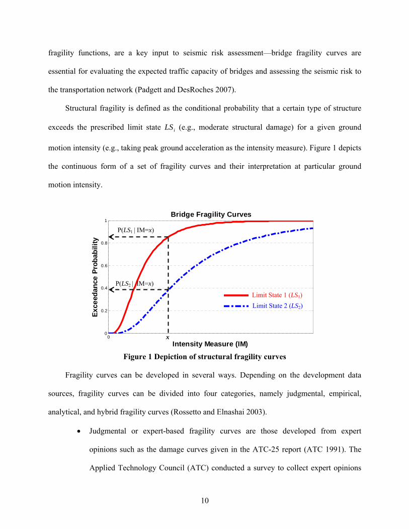
Structural fragility is defined as the conditional probability that a certain type of structure
exceeds the prescribed limit state iLS (e.g., moderate structural damage) for a given ground
motion intensity (e.g., taking peak ground acceleration as the intensity measure). Figure 1 depicts
the continuous form of a set of fragility curves and their interpretation at particular ground
motion intensity.
00
0.2
0.4
0.6
0.8
1
Intensity Measure (IM)
Ex
ceed
ance
Pro
bab
ilit
y
Bridge Fragility Curves
Figure 1 Depiction of structural fragility curves
Fragility curves can be developed in several ways. Depending on the development data
sources, fragility curves can be divided into four categories, namely judgmental, empirical,
analytical, and hybrid fragility curves (Rossetto and Elnashai 2003).
Judgmental or expert-based fragility curves are those developed from expert
opinions such as the damage curves given in the ATC-25 report (ATC 1991). The
Applied Technology Council (ATC) conducted a survey to collect expert opinions
x
P(LS1 | IM=x)
P(LS2 | IM=x)
Limit State 1 (LS1)
Limit State 2 (LS2)
11
for estimation of structural damage from earthquakes. The survey results were
represented in a damage probability matrix that describes probabilities of a facility
being in a specific damage state for different level of ground shaking using the
Modified Mercalli Intensity (MMI) scale. Based on the damage probability matrix,
damage curves were developed in the ATC-25 report. However, only five bridge
experts responded and offered their opinion on bridge damages. These judgmental
fragility curves from a small sample-based survey are usually sensitive to systematic
sampling errors and prone to bias (Lindell and Perry 2000; Harrald et al. 1994).
Fragility curves can also be developed based on observations of empirical structural
damage data from past earthquakes (Basőz et al. 1999; Basőz and Kiremidjian 1996;
Yamazaki et al. 1999; Shinozuka et al. 2003). For example, empirical fragility
curves for bridge with and without retrofit were developed based on the field
inspection data collected after the 1994 Northridge earthquake (Shinozuka et al.
2003). The major limitation of empirical fragility curves is the lack of sufficient
empirical data for various types of bridges and damage levels.
In absence of adequate empirical data in the Central United States, analytical
fragility curves are developed based on the evaluation of structural response.
Various approaches have been utilized to develop bridge fragility curves. For
example, elastic spectral method (Jernigan and Hwang 2002) and capacity spectrum
method (Dutta 1999; Mander and Basőz 1999; Federal Emergency Management
Agency [FEMA] 2006; Werner et al. 2006) were used to develop analytical bridge
fragility curves. The analytical fragility curves developed based on non-linear time
history analysis are the most reliable (Shinozuka et al. 2000) and thus have been
12
widely adopted in recent research (Mackie and Stojadinovic 2004; Choi et al. 2004;
Elnashai et al. 2004; Nielson 2005). The applications of the analytical models are
often limited to the most critical components of infrastructure systems (i.e., bridges
in transportation systems) because of their requirements for larger information and
computationally expensive analysis (Eguchi 1984).
Hybrid fragility curves combine data from various sources and compensate for the
scarcity of observational data, subjectivity of judgmental data, and modeling
deficiencies of analytical procedures (Jeong and Elnashai 2007).
With structural fragility curves, the damage probabilities of the components in
transportation infrastructure systems at a particular ground shaking intensity can be obtained.
The post-earthquake traffic carrying capacity of a component of transportation network (e.g.,
bridge) will be time-dependent in accordance to the structural damage and restoration of the
component, as defined by the damage-functionality relationship.
2.1.2.2 Damage-Functionality Relationship
The damage-functionality relationship defines the residual traffic capacity of a component
for a particular damage state. In other words, the damage-functionality relationship maps the
structural damage states to the reduced traffic throughput capacities due to bridge collapse and
lane or road closure, etc. Once the functionalities of components in the network are obtained, the
time-dependent system functionality that corresponds to the level of serviceability or traffic
carrying capacity can be determined.
Similar to the approaches used for developing fragility curves, there are three ways (i.e.,
empirical, analytical, and expert opinion-based) to develop the damage-functionality
relationships.
13
The first category of damage-functionality relationship is based on empirical data.
Observations of repair and restoration and corresponding structural damage from past events are
used to develop the relationship. This empirical approach, as indicated previously, requires
sufficient field observations for various types of structures from past earthquakes. Though this
empirical approach could be effective in regions with adequate observation data, it would be
difficult for regions with little seismic data, e.g., the Central United States.
In addition to the empirical approach, bridge damage-functionality relationship can be
developed analytically by using statistics of structural damage repair and restoration for the
regions with adequate observation data (e.g., California). Mackie (2004) investigated analytical
damage-functionality relationship for typical bridge types in California, in which the
functionality of a bridge was measured by its load carrying capacity. This approach, however, is
not representative because it does not reflect the repair or road closure decisions.
Expert opinion-based approach has been widely employed because it is easy to implement
and effective to capture the subjective nature of bridge functionality that is based on closure and
repair decisions. This approach was used in the ATC-13 (ATC 1985) to evaluate the loss of
functionality and estimate the restoration time for lifeline facilities including transportation
infrastructures. To collect the responses from professionals, a survey questionnaire was
administered to query the participants about the time elapsed before restoring 30%, 60% and
100% functionality at a given bridge damage state. Though only four participants responded to
the bridge survey, these results were later used in HAZUS to establish discrete and continuous
restoration curves (FEMA 2006). Targeting the continuous multi-span concrete bridges in the
Mid-America region, Hwang et al. (2000) conducted a survey to collect expert opinions on
stepwise restoration curves, in which only nine responses were received. More recently, Padgett
14
and DesRoches (2007) performed a web-based survey to collect expert opinions from
experienced staffs in the departments of bridge engineering maintenance and operations of the
Central and Southeastern United States (CSUS). About 75% experts responded to the survey and
the damage-functionality relationship was obtained for the CSUS bridges based on 28 samples.
The drawback of these expert-based relationships is that they are subjective and biased (Lindell
and Perry 2000; Harrald et al. 1994). In addition, the discrete relationships are limited due to the
stepwise function form with the assumption of discrete levels traffic carrying capacity.
2.2 Performance Modeling and Evaluation of Transportation Systems
The need to protect critical transportation infrastructures from extreme events has attracted
increasing research focus for the past twenty years. The contexts of these studies range from
emergency response and disaster evacuation (Jha and Behruz 2004) to disaster recovery and
mitigation (Murray-Tuite and Mahmassani 2004; Basőz and Kiremidjian 1996; Kim et al. 2008;
Liu et al. 2009). In every context, a system performance metric is needed to evaluate the
performance or serviceability of a road network and compare the effectiveness resulted from
various intervention or mitigation projects. Such system metrics for transportation networks can
be divided into three broad categories: (i) travel delay cost, (ii) network flow capacity, and (iii)
reachability (or connectivity).
The first category of metrics (i.e., travel delay cost) depends upon origin-destination (OD)
demand that describes number of vehicle (or person) trips between locations (i.e., origins and
destinations) in the road network; while the latter two categories are OD-independent. OD
demand reflects number of households, income distribution, vehicle ownership, employment
statistics, zoning, and retail-activities. OD demand can be obtained either from surveys and
automatic vehicle identification data, or by mathematical modeling.
15
2.2.1 Travel Delay Cost
Travel delay cost metrics have been widely used in assessing the seismic risk of
transportation systems (Kiremidjian et al. 2007; Nojima and Sugito 2000; Kim et al. 2008). The
travel delay cost metrics can be given by modeling traffic flow distribution and travel time (i.e.,
travel costs) over road networks in the traffic assignment step of the conventional four-step
transportation demand forecasting process (Weiner 1987).
Traffic assignment methods (static or dynamic, user equilibrium or system optimal) have
been one of the most widely used approaches to model traffic flow over road networks since the
first mathematical formulation of static traffic assignment problem was proposed by Beckmann
and colleagues (1956). Traffic assignment models require detailed OD demand and traveler
routing rules as the input. Based on the assumptions on traffic demand and link cost, traffic
assignment models can be grouped into two broad categories: static and dynamic assignment
models.
2.2.1.1 Static Traffic Assignment Models
A static traffic assignment model assumes the model parameters (e.g., traffic demand and
travel cost) do not vary over time. The static models give steady state traffic flow in user
(traveler) equilibrium (UE), in which no traveler in the network can unilaterally change routes
and improve his or her travel time thereby (Wardrop 1952; Sheffi 1985).
Based on the assumptions on the behavior of drivers in their route choices, static traffic
assignment models can be further categorized into two groups: (i) deterministic user equilibrium
(DUE) model, and (ii) stochastic user equilibrium (SUE) model.
The DUE model assumes the driver always choose the shortest path, while the driver’s
route choice is stochastically determined in the SUE model. The assumption of DUE model on
16
driver’s route choice is reasonable in urban road networks since the driver tends to minimize his
or her individual travel time. Therefore, it has been widely used to study the driving behavior in
urban area (Sheffi 1985). SUE assumes the driver chooses his or her route based on individual
preference, which can be measured with the stochastically generated utility or attractiveness. The
SUE model is especially useful for traffic planning in rural areas where traffic is less congested
compared with urban areas, and where not all drivers choose the shortest paths (Sheffi 1985;
Taplin 1999). Additionally, stochastic models can be employed to simulate optimal egress
problem during an emergency such as a fire or earthquake by characterizing the mixing and
confluence of exiting user streams, bottlenecks, slowdown due to hazard prorogation, and
blocking (Talebi and Smith 1985).
Static assignment model provides a fairly good and efficient prediction of the average travel
time and therefore has been widely accepted and employed by many transportation agencies and
practitioners (Kim et al. 2008). In a seismic risk study for a Japanese transportation network,
Nojima and Sugito (2000) evaluated its post-earthquake functional performance based on the
travel costs, which were simulated by a static traffic assignment model. Kim et al. (2008)
evaluated the seismic impact on the road network in Charleston, South Carolina with the static
traffic assignment model (DUE), in which the network performance was measured by the total
system travel time. Viswanath and Peeta (2003) also employed the traveling (routing) cost of OD
pairs as the performance metric to identify critical routes for earthquake response with a multi-
commodity maximal covering network design problem (MCNDP) formulation. In a recent study
by Liu et al. (2009), travel delay cost is taken as one of two effectiveness metrics for measuring
the benefit of bridge retrofit.
17
Although the UE model with inelastic demands (i.e., fixed OD trips) is adequate to model
the region-wide traffic flow (Werner et al. 2006) under normal conditions, its unrealistic static
assumption of the traffic information and drivers’ behavior (Ran and Boyce 1996) make it
impossible to account for dynamics of travel demand and traffic congestion after extreme events.
For example, the model cannot provide adequate estimate of traffic along specific highway links.
As indicated in a validation experiment of traffic flow after the Northridge Earthquake (Werner
et al. 2006), the fixed-demand UE model overestimated the travel time (per trip) ten times the
observed travel time from local traffic reports on some highway segments (i.e., near bridge
collapse at I-10/La Cienega, SR-119/Gothic, and I-5/SR-14) (Caltrans 1995).
2.2.1.2 Dynamic Traffic Assignment Models
In addition to static traffic assignment models, the travel delay cost performance metrics
have also been employed in dynamic traffic assignment (DTA) models to compute the average
travel time or clearance time under extreme events.
DTA models provide an alternative way to address the unrealistic issues with the static
assignment models. Instead of assuming static traffic demand, the DTA models take into account
the fluctuation of road traffic by introducing time-dependent traffic flow and route choices. The
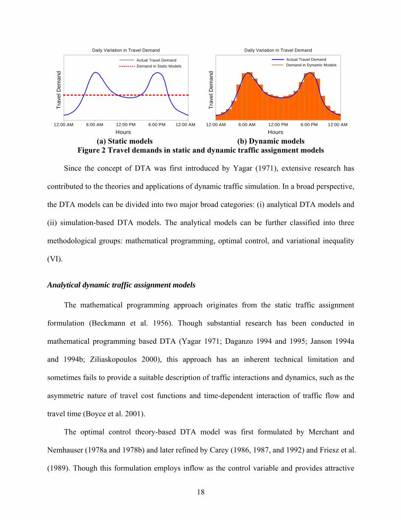
differences of travel demand assumption between static and dynamic assignment models are
illustrated in Figure 2.
18
(a) Static models (b) Dynamic models
Figure 2 Travel demands in static and dynamic traffic assignment models
Since the concept of DTA was first introduced by Yagar (1971), extensive research has
contributed to the theories and applications of dynamic traffic simulation. In a broad perspective,
the DTA models can be divided into two major broad categories: (i) analytical DTA models and
(ii) simulation-based DTA models. The analytical models can be further classified into three
methodological groups: mathematical programming, optimal control, and variational inequality
(VI).
Analytical dynamic traffic assignment models
The mathematical programming approach originates from the static traffic assignment
formulation (Beckmann et al. 1956). Though substantial research has been conducted in
mathematical programming based DTA (Yagar 1971; Daganzo 1994 and 1995; Janson 1994a
and 1994b; Ziliaskopoulos 2000), this approach has an inherent technical limitation and
sometimes fails to provide a suitable description of traffic interactions and dynamics, such as the
asymmetric nature of travel cost functions and time-dependent interaction of traffic flow and
travel time (Boyce et al. 2001).
The optimal control theory-based DTA model was first formulated by Merchant and
Nemhauser (1978a and 1978b) and later refined by Carey (1986, 1987, and 1992) and Friesz et al.
(1989). Though this formulation employs inflow as the control variable and provides attractive
Tra
vel D
ema
nd
Hours
12:00 AM 12:00 AM6:00 PM12:00 PM6:00 AM
Actual Travel Demand
Daily Variation in Travel Demand
Demand in Dynamic Models
Tra
vel D
ema
nd
Hours
12:00 AM 12:00 AM6:00 PM12:00 PM6:00 AM
Actual Travel Demand
Demand in Static Models
Daily Variation in Travel Demand

19
explicit relationship between exit flow and link flow, it requires (i) the exit flow function be
convex to establish an optimal control model with multiple OD pairs, and (ii) the exit flow rate
be positive to satisfy exit flow function and provide realistic flow propagation. In addition, this
formulation suffers from limitations such as the lack of explicit constraints to ensure first-in-
first-out (FIFO) of traffic propagation on transportation networks and preclude holding of
vehicles at nodes, the lack of a solution procedure for general networks (Peeta and
Ziliaskopoulos 2001).
Compared with mathematical programming and optimal control, VI provides a more
general platform with analytical flexibility and convenience to address various dynamic traffic
assignment problems (Peeta and Ziliaskopoulos 2001; Boyce et al. 2001; Nagurney 1998; Friesz
et al. 1996). Therefore, this approach has gained increasing attention for both static and dynamic
network modeling since it was first introduced by Dafermos (1980) for the static traffic
equilibrium problems. However, VI is computationally intensive, raising issues of computational
tractability for real-time deployment, especially for the path-based VI formulation that requires
complete path enumeration (Peeta and Ziliaskopoulos 2001).
Despite their capacities to describe spatio-temporal interactions and traffic flow propagation
in an abstract mathematical manner, analytical traffic representations that adequately replicate
theoretic time and flow relationship and yield well-behaved formulation of DTA models are
currently unavailable, due to the issues of traffic realism and intractable computational cost
arising in the context of complex transportation networks (Peeta and Ziliaskopoulos 2001; Boyce
et al. 2001).
20
Simulation-based dynamic traffic assignment models
In the context of real-world deployment, simulation-based models have gained greater
acceptability (Yang 1997; Mahmassani 2001). Simulation-based DTA models use traffic
simulators to model the complex dynamics of traffic flow and determine traffic propagation on
the network. Several simulation-based DTA models are available, including the DYNASMART
(Mahmassani and Peeta 1995), the DYNAMIT (Ben-Akiva et al. 1997), and the VISTA
(Ziliaskopoulos and Waller 2000). The key limitations of simulation-based DTA model are that:
(i) it is unable to derive the associated mathematical properties through simulations, and (ii) the
computational burden associated with the use of traffic simulator in a real-world deployment
could be operationally restrictive (Peeta and Ziliaskopoulos 2001).
Thus far, only a handful studies established the link between the travel cost metrics and
disaster management by using dynamic transportation systems modeling, though DTA model has
evolved rapidly and been used in real-time traffic operations, traffic planning and management
practices (i.e., intelligent transportation systems). Such metrics have been used to identify the
most vulnerable road segments (Murray-Tuite and Mahmassani 2004), evaluate the effectiveness
of evacuation strategies during emergency evacuation (Tuydes and Ziliaskopoulos 2006; Jha and
Behruz 2004), or determine the spatial distribution and capacities of hurricane shelters (Anil and
Ozbay 2007).
The travel delay cost metrics are highly dependent on origin-destination demand
information. During the short-term response period of a disaster (usually within the first few
days after the impact), however, the post-disaster traffic behavior and demand (i.e., route choices)
could change dramatically (Theodoulou and Wolshon 2004; Werner et al. 2006). The traffic is
most likely under the central control of the transportation management agencies (TMA) (Murray-
21
Tuite and Mahmassani 2004). For example, post-earthquake travel demand could alter
substantially due to travelers’ reaction to bridge damage, road closures, and congestions—many
travelers are unwilling to endure the travel delay and could eventually forego their trips (Werner
et al. 2006). The difficulties of obtaining realistic traveler route choice behavior, in addition to
the computational challenges associated with traffic simulation on complex networks, make
travel delay cost an unrealistic metric for modeling network behavior during the short-term
emergency response period.
2.2.1.3 Travel Demand Modeling
An alternative approach to address the issue of inelastic trip demand is to introduce more
realistic post-earthquake travel demand models to characterize the changes in traveler’s behavior
and routing choices. The following subsections provide a review of existing travel demand
models under post-earthquake situations and evidences from recent major earthquakes in both
U.S. and Japan.
Travel demand modeling, as part of the conventional four-step urban transportation demand
forecasting process (Weiner 1987), is to establish spatial distribution of travel between traffic
analysis zones (TAZ). In other words, travel demand modeling explains where the trips originate
from and where they go, with what travel modes and routes. Since a survey of actual travel
demand would be either extremely expensive or impossible at all, the travel demand modeling is
mostly carried out with simulation approaches.
Traffic modeling in extreme events was first studied in the 1970s for hurricane evacuation.
The focus was shifted to nuclear power plant evacuation after the 1979 Three Mile Island
accident but was directed back to hurricanes again in the 1990s. Earthquakes-related traffic
modeling has drawn attention lately, especially after the recent tsunamis and earthquakes in Asia.
22
Review of existing travel demand models
Though many simulation packages are available to model traffic under normal conditions
(e.g., CORSIM, VISSIM, and EMM/2), only a handful models have been developed for use in
emergency conditions. These include, but not limited to, the Oak Ridge Evacuation Modeling
System (OREMS), the Dynamic Network Evacuation (DYNEV), Transportation Emergency
Management of Post-Disaster Operations (TEMPO), and the Evacuation Traffic Information
System (ETIS). Other similar evacuation packages include NETVAC (Sheffi et al. 1981),
HURREVAC (USACE 1994), and MASSVAC (Hobeika and Jamei 1985).
OREMS is designed to estimate evacuation time and develop traffic management strategies
under different events or scenarios (Rathi and Solanki 1993; ORNL 2002; Chang 2003). OREMS
can be used to identify evacuation routes and identify bottlenecks as well as to assess the
effectiveness of alternative traffic control and evacuation strategies (Moriarty et al. 2007).
DYNEV was traditionally developed to simulate the evacuation from nuclear power plant, but
later enhanced for modeling hurricane evacuations (Moriarty et al. 2007; Chang 2003; Mei 2002).
ETIS is a transportation simulation tool developed by the U.S. Department of Transportation to
forecast large cross-state traffic volume for hurricane evacuation (Chang 2003; Wolshon et al.
2005; PBS&J 2003).
Both OREMS and DYNEV require similar TAZ-based inputs such as population of
residents, employment/income, and number of vehicles per dwell unit. Users need define
parameters of behavior patterns (participation rate), day of year/time of day, and basic weather
conditions. Gravity models are used in both OREMS and DYNEV during the trip distribution
step. The difference between OREMS and DYNEV is that DYNEV includes mode-split step and
assumes static assignment (Chiu et al. 2005). ETIS requires county-based inputs such as the
23
population of residents/tourists and the destination percentage of evacuees for each county.
Travel demand is manually generated during trip distribution period. Sigmoid curve loading
model (Yazici and Ozbay 2008; Fu 2004) is employed to simulate time-dependent behavioral
response in ETIS.
The staged model (Southworth 1991; Wilmot and Mei 2004; Moriarty et al. 2007) is the
most widely accepted approach to describe the traffic demand modeling under hurricane and
nuclear hazards. The first stage is to estimate travel demand by using the number of at-risk
population and its response to evacuation orders (Wilmot and Mei 2004); then trip distribution
models are employed to generate trip matrix with gravity model or manual assignment. The
second stage, also known as network loading stage (Southworth 1991), is to load the travel
demand to the transportation network with models that simulate the departure time.
Modeling the travel demand and traffic following earthquakes is much more complex than
hurricane or nuclear-related hazards, partially due to the fact that post-earthquake travel demand
is coupled with the deteriorated capacity of post-earthquake transportation infrastructures.
Additionally, public response to earthquake is distinct because prior warning for earthquakes is
usually unavailable or infeasible, which makes the post-earthquake traffic pattern less dependent
on the behavioral response or network loading model.
TEMPO is a decision support system developed during the aftermath of the 1989 Loma
Prieta earthquake, which specifically addresses the transportation needs following a major
earthquake such as emergency vehicles and repair crew routing and traffic diversion (Ardekani
1992b). The post-earthquake demand model used in TEMPO, however, is solely based on the
physical damage of transportation infrastructure (i.e., the closure of roads) and does not consider
the changes of travel behavior after the earthquake impact.
24
It has been noted that the pre-earthquake travel demand was inappropriate for evaluating
the post-earthquake performance of transportation networks (Fan 2006; Shinozuka et al. 2005;
Kiremidjian et al. 2007). The change of post-earthquake travel patterns has been taken into
account when evaluating the performance of transportation systems (Shinozuka et al. 2005;
Kiremidjian et al. 2007). Other related research on long-term travel demand change under
earthquake impact has been conducted with multi-regional input-output models (Ham et al.
2005a and 2005b; Kim et al. 2002).
The approaches and models that reflect short-term post-earthquake travel pattern changes
can be grouped into two broad categories: (i) model trip demand changes by modifying the pre-
earthquake normal OD matrix (Shinozuka et al. 2005; Wakabayashi and Kameda 1992); and (ii)
employ alternative assignment models such as the modified incremental assignment method
(Nojima and Sugito 2000) and the Variable Demand Model (VDM) (Fan 2006; Kiremidjian et al.
2007).
Shinozuka et al. (2005) estimated the post-earthquake demand matrix by modifying the pre-
earthquake origin-destination data. They introduced trip reduction factors by building occupancy
and trip purposes to account for zonal trip activity changes due to building damage from ground
shaking. Then a combined assignment and distribution models were employed to predict post-
earthquake travel delay. However, essential influencing factors such as emergency shelters and
release of hazardous materials (HAZMAT) were not addressed in their study. The reduction
factors are also limited, as they require additional information such as the type of trip purpose
(e.g., home-based work trips or home-based school trips) that may not be available in all traffic
planning organizations.
25
The similar idea of using travel demand modifiers was also employed in some other recent
research to incorporate the changes of travel demand and reduction of road capacities due to
seismic damage. For example, Kim (2009) designed post-earthquake emergency scenarios that
incorporate demand changes due to HAZMAT release and emergency shelters—areas with
HAZMAT release were taken as repellent zones where link capacities are reduced to 1% of their
original values; areas with shelters are taken as attraction zones with an additional 30% demand.
Wakabayashi and Kameda (1992) estimated the post-earthquake OD matrix due to the Bay
Bridge closure after the Loma Prieta earthquake, by linking the link flow data from eight traffic
observation sites and the census population data. The highway system in the San Francisco Bay
Area was simplified into a 23-node network and the gravity model was employed to distribute
the vehicle trips. This approach, however, did not consider the building damage information, nor
did it account for other demand changing factors such as shelters and HAZMAT release.
Another category of approach to modeling post-earthquake trip demand is to reflect the
demand changes with alternative traffic assignment models (Fan 2003; Werner et al. 2006;
Kiremidjian et al. 2007). Nojima and Sugito (2000) proposed the modified incremental
assignment method (MIAM), an alternative assignment model to obtain the post-earthquake OD
matrix. MIAM loads the damaged network with pre-earthquake OD trips and the output OD-
matrix from the modified method is different from the pre-earthquake one because part of the
OD trips may not be satisfied due to physical isolation of centriods, overload, and/or congestions
(Nojima and Sugito 2000). This method, however, can only provide an approximate solution and
generally is not able to find equilibrium solutions (Lu 2006).
In a study to evaluate the earthquake risk to transportation system in the San Francisco Bay
Area, Kiremidjian et al. (2007) defined the user equilibrium with a variable-demand model
26
(VDM) and compared the travel delays resulting from damage to ground shaking with a fixed
demand model (or FDM). The VDM provides a relative reasonable assumption of elastic travel
demand (DfT 2006), e.g., the travel demand decreases as the travel time between OD-pairs
increases because of reduced link capacity; while the fixed demand model assumes the travel
demand is unchanged before and after the earthquake. It was found that: (i) post-event travel
times increase significantly with FDM assumption, and (ii) the travel times remain relatively
unchanged and decrease with VDM assumption. These findings confirm the field observations
after the Northridge Earthquake (Werner et al. 2006). REDARS 2 also employs the VDM model
to account for the post-earthquake travel demand change (Werner et al. 2006).
Though the VDM models are able to represent the post-earthquake changes of travel pattern
to some extent, two major underlying assumptions may limit the application of the VDM models
in California only, because (i) the assumption of reduced network traffic capacity would cut trip
demand (Kiremidjian et al. 2007) and increase travel time may not be true for all OD-pairs, and
(ii) the predicted equilibrium OD-pair travel time may not always fall on the demand curves
(Werner et al. 2006). The VDM analysis by Kiremidjian et al. (2007) assumes that traffic
demand decreases as observed following both the 1989 Loma Prieta and 1995 Northridge
earthquakes (Yee and Leung 1996a and 1996b; Werner et al. 2006). This assumption of
decreased post-earthquake demand is based on the commuters’ behavior in the study region only
and thus the findings are pertain to traffic patterns observed in California. Traffic patterns could
be completely different in other regions or countries—the travel demand significantly increased
following the 1995 Kobe earthquake due to unique rerouting conditions (Kiremidjian et al. 2007).
27
Evidences from recent earthquakes
This section presents the observed changes of traffic patterns following major historic
earthquakes in the United States and Japan, including the 1989 Loma Prieta earthquake, the 1994
Northridge, the 1995 Hanshin-Awaji earthquake, and the 2004 Niigate Ken Chuetsu earthquake.
These two countries are chosen because both countries have well-developed transportation
infrastructures as well as high seismic risks.
Loma Prieta earthquake (U.S.)
Transportation network was the hardest hit infrastructure system in the 1989 Loma Prieta
earthquake ( wM 6.9). The major disruptions of highway service were in San Francisco, Oakland,
and the major bridges between the two cities. The collapse of a section of the Bay Bridge
seriously impacted the Bay Area travel. The cross-bay traffic volumes on other major bridges
increased significantly after the earthquake—post-earthquake traffic volume on the San Rafael
Bridge increased by 79.9% than the pre-earthquake volume (Housner and Thiel 1990). As a
result, approximately 0.3 million commuter traffic (EQE 1989) had to use alternate city surface
streets for nearly three years after the earthquake (Ardekani 1992a). Surface streets in San
Francisco were also struck heavily—the hardest hit Marina District in the City of San Francisco
was evacuated immediately after earthquake and public access was restricted.
Northridge earthquake (U.S.)
Though the 1994 Northridge earthquake ( wM 6.7) is one of the costliest earthquakes in U.S.
history and the ground acceleration was the highest ever instrumentally recorded in an urban
region in North America (SCEC n.d.), damage to the highway structures was not enormous due
to the $1.5 trillion retrofit program in California. The earthquake caused major damage on the
following four freeways and interchanges: Interstate 5 (I-5, the Golden State Freeway), Interstate
28
10 (I-10, the Santa Monica Freeway), State Route 14 (SR-14, the Antelope Valley Freeway), and
State Route 118 (SR-118, the Simi Valley Freeway). Minor damages also occurred at many other
locations, but none of the damage-incurred closures at these locations lasted more than a few
weeks. Most parts of the local street network were not significantly affected by the earthquake.
Among the four significant freeway damage locations, damages at two locations, namely
SR-14/I-5 interchange and I-10 are notable (Boarnet 1996). The damage at SR-14/I-5
interchange that links the residential suburb in Santa Clarita Valley and the City of Los Angeles
left more than 280,000 commuters with little choice but to take detour and endure traffic delays
that were initially greater than an hour during peak periods (Barton-Aschman and Associates
1994; Ardekani 1995).
Except for the first few days after the earthquake, excessive delays were not experienced
and the transportation systems in Los Angeles continued to function throughout the
reconstruction period (Yee and Leung 1996a and 1996b). The area wide traffic volumes
substantially decreased than normal during the first few days following the earthquake. Travel
delays were substantial in the first few days following the earthquake (EQE 1994), although
alternative travel modes (e.g., public transit) were taken (Debban 1995). The travel demand
increased dramatically within in the following week because workers began returning to their
jobs, but still lower than normal. After the first week, although congestion was bad in some
places, excessive congestion was not experienced except for the Santa Cruz area, which was
isolated due to lack of redundancy (Webber 1992; Tsuchida and Wilshusen 1991). During the
first month, most delays were greater than thirty minutes. Many damaged freeways were repaired
within a few months of the Northridge Earthquake. By March of 1994, the travel demand during
the peak hours stabilized throughout the area (Yee and Leung 1996a) and delays on most
29
transportation corridors stabilized at five to twenty minutes (Barton-Aschman and Associates
1994).
Note that the short-term changes in travel pattern were not entirely commuters’ responses to
transportation system disruptions—many people stayed at home for the week following
earthquake (Schmitt 1998). Moreover, because the earthquake occurred very early on the Martin
Luther King Day, a U.S. national holiday, many trips would not have occurred anyway.
Great Hanshin (Kobe) earthquake (Japan)
The 1995 Hanshin-Awaji earthquake ( wM 6.8) in the Osaka-Kobe area had an even greater
impact on the transportation systems compared with the Loma Prieta and Northridge earthquakes
in the U.S. The span collapses of the elevated Osaka-Kobe expressway (Route 3) caused long-
time closure of this major transportation corridor. The travel demand surged following the
earthquake (Kiremidjian et al. 2007). In addition, parallel routes also suffered major damage to
bridges and elevated section of both the Shinkansen and commuter rail lines (Buckle and Cooper
1995).
Niigate-Chuetsu earthquake (Japan)
In the 2004 Niigate Ken Chuetsu earthquake ( wM 6.9), transportation systems such as the
Shinkansen (the Japanese high-speed rail network) and expressways were significantly disrupted,
especially in the Chuetsu region. The overall performance of the transportation systems, however,
was good (Ashford and Kawamata 2006) partially because detour routes contributed to
interregional travel and commodity flow (Tatano and Tsuchiya 2008). Until the 13th day after
the earthquake, freight transit time between Tokyo (Kanto region) and Niigate increased by 25%
and business travel cost by 9%-30%. It took two weeks to reconstruct the damaged expressways
and two months for the Shinkansen to resume operations (Tatano and Tsuchiya 2008).
30
The observed impact on the performance of transportation systems and post-earthquake
travel patterns from the recent U.S. and Japanese earthquakes suggest that, firstly, transportation
infrastructures are especially vulnerable to earthquake impact and many of the disruptions to
transportation systems are due to damages to bridges or viaducts. In addition, transportation
corridors linking suburban residential areas to downtown region, if damaged, are prune to
significant delays. Transportation networks with less redundancy could lead to serious traffic
problem, as observed in the Santa Cruz area in Loma Prieta earthquake. Furthermore, post-
earthquake travel demand is transient, which could change drastically (surge or decrease) during
the first few days or weeks following an earthquake. The travel demand may need a few months
to stabilize—people are willing to travel as the post-earthquake recovery actions are taken (e.g.,
repair or reconstruction of damaged bridges and/or roadways). Finally, post-earthquake travel
patterns are distinct in different regions, as was found in the California and Kobe earthquakes.
2.2.2 Network Flow Capacity
As an alternative to the travel cost-based metrics, network flow capacity (Nojima 1998;
Chen and Tzeng 1999) can be used as a performance metric of transportation networks.
Maximum flow is the largest possible flow between source nodes and sink nodes without
exceeding the capacity of any link in the network (Ahuja et al. 1993).
This metric is an obvious property of the network itself, and is hence independent of the
traveler behavior and OD demand. Compared with the travel delay cost metric, the network flow
capacity metric is employed in a relatively smaller number of studies. Nojima (1998) evaluated
the post-earthquake serviceability of a transportation network, in which the maximum flow
capacity was used to find Birnbaum’s importance measure for the network links. Nojima’s
maximum flow capacity, however, is rather an intermediate measure that was used to find
31
Birnbaum’s probabilistic importance than a system-level performance metric. Feasible flow
capacity, a variation of the maximum flow capacity, was used as one of the measures in a post-
earthquake road network reconstruction-scheduling problem (Chen and Tzeng 1999). The
feasible flow capacity is taken as one of the objectives in the formulated multi-objective
optimization model. Lee et al. (2010) estimated the post-hazard traffic flow capacity of a bridge
transportation network, in which the flow capacity is given by a standard maximum flow
algorithm. In these studies, the network flow capacity-based formulation, however, did not
account for the resource constraints, nor did they include the bridge components in the
transportation systems. Although some research has been done, to the best of our knowledge,
such network capacity metrics are not currently considered in seismic retrofit planning to
improve the emergency flow capacity of a transportation network in immediate population
evacuation scenarios.
2.2.3 Reliability of Network Reachability
Defined as being able to get from one vertex in a digraph to some other vertex in graph
theory, the reliability of network reachability (also know as connectivity reliability) is one of the
most frequently used measures for networked systems. For transportation systems, the
connectivity denotes the reachability of an arbitrary node-pair via at least one path. Connectivity
highly depends on the post-earthquake completeness or connectedness of a transportation
network and hence it is suitable for the case of immediate post-disaster humanitarian aid. The
network systems’ traffic capacities, travel times, and trip lengths, however, are ignored in the
reachability analyses. Instead, the reachability analyses seek only to determine whether, or with
what probability, a path remains operational (or connected) between the given sources and
destinations (Rojahn et al. 1992). If the path (or paths) connects the selected node-pair following
32
an impact, serviceability (or performance) analyses seek additional information on the remaining
or residual capacities that can be found mathematically by convolving component capacities with
infrastructure completeness (Rojahn et al. 1992).
Considerable advances have been made in the field of network connectivity and various
algorithms proposed to analyze the network reliability since the 1970s'. These network reliability
analysis algorithms can be grouped into two broad categories: (i) simulation-based algorithms
(e.g., Monte Carlo simulation), and (ii) analytical algorithms (e.g., the decomposition methods
and binary decision approaches).
2.2.3.1 Simulation-Based Algorithms
Simulation-based algorithm such as Monte Carlo simulation (MCS) is one of the most
widely accepted approaches to evaluate system connectivity. These algorithms do not rely on
analytical models or graphical representation—all information needed to implement simulation is
the component reliabilities and network configuration (e.g., network topology). Because of its
simplicity of implementation, MCS is widely used in many engineering applications when
analytic approaches are not feasible. Though MCS cannot give exact solution and take longer
time to converge, the results are fairly good and close to exact solutions. Therefore, MCS is
widely accepted as an alternative approach to validate the results obtained in other ways.
Employing MCS approach to evaluate the connectivity reliability of a network is
straightforward—first, random numbers following the uniform distribution (0,1)U are generated
to simulate failures of network components; then graph search algorithms (e.g., the breadth-first
search [BFS]) are used to determine the connectivity of node-pair in the network. This process is
repeated for thousands of times or more and the frequencies of connectivity are takes as network
reliability. In general, a mid-size network requires two thousand to ten thousand of simulation
33
runs and a larger network ten thousand to one hundred thousand of runs to converge a stable
reliability estimate (Li 2005).
MCS is easy to implement and can be applied to any size and any types of networks. MCS
has been extensively used to evaluate utility systems’ connectivity. Oppenheim (1977) simulated
seismic damage of water delivery systems and transportation networks with Monte Carlo
simulation-based method. Shinozuka et al. (1981, 1992, 1996, and 2003) employed MCS to
assess seismic reliability of various infrastructure systems, including water delivery networks,
highway networks, and power networks in Tennessee and California.
However, the shortcomings of simulation-based MCS are also obvious. Firstly, the
convergence is not controllable. It could take thousands of simulation runs to get a stable result,
and the number of simulations to achieve convergence is sensitive to component reliability. In
addition, MCS is based on the independence assumption of component failure and thus difficulty
to account for the dependence between infrastructure systems and their components. Furthermore,
MCS is the least economical way to evaluate network reliability and usually take much longer
time than other approaches. Lastly, the results given by MCS are not informative and limited to
the estimation of reliability only.
Although the simulation-based algorithms are easy to implement and are applicable to large
networks, they are computationally inefficient and usually incapable of controlling the accuracy.
In contrast to the simulation-based algorithms, the analytical ones are able to give exact or more
accurate results with less time consumption for small-scale networks. The following section
provides a review of analytical algorithms for network reachability calculation.
34
2.2.3.2 Analytical Algorithms
The fundamental idea of analytical approach for network connectivity is to convert a
complex network to combination of simply networks such as parallel or series systems; and then
system connectivity could be computed by finding the union and intersection of these simply
networks, e.g., a generic substation can be modeled with a series system of macro-components
(Vanzi 1996).
Kroft (1967) first proposed the shortest path-based algorithm to compute the network
connectivity reliability. Panoussis (1974) and Taleb-Agha (1975 and 1977) demonstrated that
general connectivity reliability can be computed by converting complex infrastructure networks
to SSP (series systems in parallel) networks. Aggarwal and Misra (1975) proposed a disjoint
shortest path algorithm. However, these methods are constrained to small networks due to the
complexity of large network systems. Based on the idea of disjoint path searching, researchers
(Dotson and Gobien 1979; Yoo and Deo 1988; Torrieri 1994; He and Li 2001; Li and He 2002)
later improved this algorithm and found it can give exact connectivity for large complex
networks. The full-probability analytic algorithm (Wu and Sha 1998) and the ordered binary
decision diagram (OBDD) algorithm (Kuo et. al 1999) are also able to find exact network
reliability but neither of them is able to handle large networks.
Connectivity between node-pairs can be evaluated based on the network configuration with
graph theory. The connectivity reliability can then be assessed if the reliability information of
network components is available. The recursive decomposition algorithm (RDA) is a method to
evaluate seismic reliability for large infrastructure systems (Li and He 2002). Using the De
Morgan’s rule and disjoint theorem (Aggarwal and Misra 1975; Ahmad 1982; Liao 1982; He and
Li 2001; Li and He 2002), the RDA recursively decomposes the network into sub-graphs until
35
there is no path existed between the source-terminal node-pair in all the sub-graphs. It is
noteworthy that the RDA is not aiming at finding all the disjoint link or cut sets but rather
estimating system reliability or failure probability (Chang and Song 2007). In addition, this
algorithm will face difficulties in finding all the disjoint link/cut sets for large complex networks.
In such cases, the RDA gives an approximate solution with reliability bounds instead by
terminating the decomposition process with a predefined allowable error (e.g., 0.1%).
On the other hand, since complete information is not always available, especially for
complex systems, researchers chose to approximate system reliability with reliability bounds.
Ditlevsen (1979) gave the theoretical bounds for general system reliability problems. However,
the theoretical bounds are often too wide to be of practical uses. Song et al. (2003 and 2006)
obtained much narrower reliability bounds of the reliability of power substation systems by
employing a linear programming approach. Song and Kang (2007) generalized the linear
programming approach and proposed a matrix-based system reliability (MSR) method to account
for dependence and incomplete information. This method takes advantage of matrix-based
language such as MathWorks MATLAB® to compute system reliability directly from two
vectors: the c vector, which is a representation of the combination of mutually exclusive and
collectively exhaustive (MECE) events, and the p vector, describing the corresponding event
probability. This method is efficient and easy to implement by means of “dot-multiplication”
(component-wise multiplication) with MATLAB®. The MSR method has recently been further
developed for evaluating the multi-scale system reliability of lifeline infrastructure systems
(Song and Ok 2010). One of the merits of MSR is that it could give reliability bounds when
complement information is not available. In case of complete information is available, event
vector and probability vector can be constructed to find the system reliability with MSR; when
36
complete information is difficult or infeasible to obtain, linear programming can be employed to
give the narrowest reliability bounds with incomplete information. Another important merit of
MSR is that dependence issues can be handled well through updating the p vector with
conditional probability theorem. The p vector is reusable for different system events and only
the new event vector needs to be updated. MSR is easy to implement and flexible to handle
dependence and incomplete information, making it advantageous to give more insightful results.
2.3 Hazard Mitigation for Transportation Systems
Transportation networks are spatially distributed complex systems that serve as emergency
routes for evacuation, rescue, and recovery in extreme events. The components are vulnerable in
extreme events and the system performance could suffer extensive damage and functionality loss,
as evidenced in past earthquakes and bridge collapse events. Due to the lack of resources,
decision makers are faced with the problem of choosing a group of bridges with higher
mitigation priority for retrofitting or updating.
Prioritization of bridge retrofitting or allocation resource for disaster mitigation has drawn
intensive research interests in the field of structural and transportation engineering since the late
1990s. The contexts of these studies range from emergency response such as disaster evacuation,
to disaster recovery and mitigation from terrorist attack and earthquake impact. From a broad
perspective, the existing methodologies can be categorized into two groups: (i) component-level
approach, and (ii) network-level approach. The following sections highlight the uses, advantages,
and limitations of the existing approaches in the literature.

37
2.3.1 Component-Level Approaches
Component-level approaches are usually well understood by decision makers with different
backgrounds and hence have been used intensively to provide decision-making support on bridge
retrofit or repair project prioritization. Such decisions may be made based on single or multiple
attributes, which could be subjective engineering judgments (e.g., structural appraisal ratings in
the NBI database) or natural attributes (e.g., average daily traffic). A variety of methods has been
employed to obtain prioritization, varying from simple direct ranking method to the analytical
hierarchy process (AHP).
Bana e Costa et al. (2008) developed a multi-criteria additive model to evaluate the
strategic importance of bridges and tunnels in Lisbon, Portugal. The five criteria used as
fundamental points of view are: (i) emergency response, (ii) vulnerability, (iii) public safety, (iv)
interference with other lifelines, and (v) long term economical impacts. The overall strategic
importance values of bridges and tunnels were then aggregated in an additive model with scaling
factors for the five attributes. Kusakabe (2004) employed the AHP approach to perform the
weighting and calculated the overall bridge seismic retrofit priorities based a three-level and
thirty-item hierarchy. In a study that developed retrofit program for the City of Los Angeles,
California, prioritization of the seismic bridge retrofit program was carried out with a weighted
formula based on replacement cost, condition of the bridge, traffic flow, and the year of
construction (Kuprenas et al. 1998). The bridges selected for the program were prioritized based
on a weighted seismic risk value score equation:
0.5 0.2 0.15 0.15S C O T AR F F F F (1)
where SR is the seismic risk (higher risk score indicating higher retrofit priority) , CF is the
replacement cost, OF is the overall rating coming from the City Files of Structures database
38
maintained by the Structural Engineering Division, TF is the equivalent traffic, and AF is the
year of built.
Similar weights-based approaches were employed by ATC (1983), Babei and Hawkins
(1991), and Federal Highway Administration (FHWA) (1995b) by using judgmental weights and
attributes of seismic hazard, structural resistance, fragilities of bridge structural elements (e.g.,
pier, seating, abutment, foundation), and cost of failure, etc. Note that these weights or scaling
factors are all based on engineering judgment and very subjective (FIB 2007). Therefore, these
methods were most useful as a relative measure of prioritization for clearly defined objectives or
goals (e.g., economic cost, travel delay, transportation safety, etc.) and not as an absolute
measure.
In addition, ranking-based approaches have been widely used for retrofit priority. Basőz
and Kiremidjian (1996) proposed a ranking-based bridge retrofit prioritization methodology for
emergency preparedness. The relative importance of a bridge was measured by the ranking of
bridge vulnerability as well as the importance factor accounting for network behavior (e.g.,
network connectivity between a predefined OD-pair). The maximum flow-based Birnbaum’s
probabilistic importance measure was employed to obtain the prioritization in updating seismic
performance of a road network (Nojima 1998). The Birnbaum’s probabilistic importance
measure implies the probabilistic contribution of improving component reliability to that of
system reliability (Henley and Kumamoto 1981). It can be calculated for road segment i as
follows:
( )(1 , ) (0 , )B
i i ii
PI P P
p
p
p p (2)
39
where BiI is the Birnbaum’s importance measure for i -th component, ( )P p is the system
reliability as the function of the component reliability vector 1 2{ , , }np p pp = , (0 , )iP p and
(1 , )iP p are the conditional system reliabilities given that the component (i.e., road segment)
fails or not, respectively.
The level of significance for a network component can also be ranked by the incurred
transport cost or economic loss from the earthquake impact (Sohn et al. 2003). A direct approach
was also proposed by Kim et al. (2008) to select the bridges for retrofit prioritization. This
approach calculated the relative importance of each bridge (i.e., the resultant incremental of total
system travel time by reducing of the post-earthquake traffic capacity of one bridge to 1% of its
original capacity) and then sorted the bridges by descending order of their contributions, on
which the decisions on retrofit prioritization can be made.
These previous studies focused on component-level analyses, dealing the network by
individual or a group of similar components. However, the inter-relationship of bridges in a
common network (i.e., the system behavior of transportation networks) was not taken into
account (Liu and Frangopol 2005). Past experience also suggests that the decisions made solely
based on some ranking index are highly dependent on the procedures used (Small 2000) and
often yield unsatisfactory results (Patidar et al. 2007).
2.3.2 Network-Level Approaches
Although the vital role of bridges in transportation networks has long been recognized, few
research managed to prioritize retrofit projects from a network viewpoint. Since the overarching
goal of bridge retrofit and maintenance is to improve transportation system’s performance and
40
mitigate potential impact from extreme events, network-level approaches represent a significant
advancement.
A variety of mathematical programming formulations has been used for problems of
maintenance planning of transportation infrastructures. Augusti et al. (1994) studied the
allocation of retrofit resource for seismic protection of a highway network using dynamic
programming. The objective is to maximum network connectivity at given seismic intensities
and under a budget constraint.
Since the bridge retrofit prioritization problem is similar to a nondeterministic polynomial-
time hard (NP-hard) discrete network design problem (DNDP), Kim et al. (2008) proposed a
network-based seismic retrofit (NBSR) problem formulation with variable capacity constraints
and budget constraint. To propose an optimal retrofit strategy at various budget levels during the
emergency preparedness planning process, the problem was reformulated into a multi-objective
optimization problem to facilitate decision-making process. The two objectives of NBSR are: (i)
to maximize the network performance, that is, to minimize the expected total system travel time,
and (ii) to minimize the total retrofit cost, respectively. Meta-heuristic methods such as Simple
GA (SGA) and Non-Dominated Sorting Genetic Algorithm (NSGA)-II were utilized to solve the
network design problem (NDP) formulations.
The procedures of the NBSR framework are illustrated in Figure 3. The travel delay cost
metrics were employed to provide essential information on traffic flow changes of and travel
delays that result from particular route closure due to excessive damage to key infrastructure
elements, or from the reduced traffic carrying capacity because of less severe damage (e.g., lane
closure for repair or imposed lower speed limit). The post-event system performance with “as-
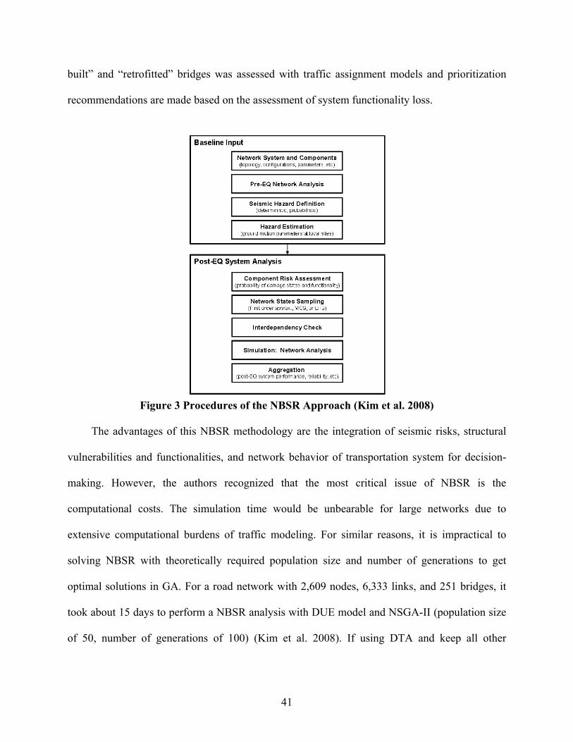
41
built” and “retrofitted” bridges was assessed with traffic assignment models and prioritization
recommendations are made based on the assessment of system functionality loss.
Figure 3 Procedures of the NBSR Approach (Kim et al. 2008)
The advantages of this NBSR methodology are the integration of seismic risks, structural
vulnerabilities and functionalities, and network behavior of transportation system for decision-
making. However, the authors recognized that the most critical issue of NBSR is the
computational costs. The simulation time would be unbearable for large networks due to
extensive computational burdens of traffic modeling. For similar reasons, it is impractical to
solving NBSR with theoretically required population size and number of generations to get
optimal solutions in GA. For a road network with 2,609 nodes, 6,333 links, and 251 bridges, it
took about 15 days to perform a NBSR analysis with DUE model and NSGA-II (population size
of 50, number of generations of 100) (Kim et al. 2008). If using DTA and keep all other
42
parameters the same, the estimated computational cost would be approximately one year
(15 24 360 days).
2.4 Summary
This chapter provides a review of previous studies on component vulnerability assessment
of transportation networks, system performance metrics, and hazard mitigation for transportation
infrastructure systems.
Particularly, relevant literature for three major categories of performance metric is
presented to highlight their computational methodologies, applications, and limitations.
Decision-making in disaster management of transportation systems is often based on the system
performance of transportation networks, which is essential for system-wide strategic mitigation
resource allocation, loss estimation, and emergency management.
Among the three categories of metric, travel delay cost is one of the most commonly used
performance metrics that provide an overall measure of the total transportation cost of all drivers.
However, this OD demand-dependent metric is usually suitable for evaluating traffic
performance under normal conditions due to (i) the lack of information on post-earthquake travel
demand (e.g., difficulties of modeling the dramatically changed post-earthquake travel behavior
and demand); (ii) the implicit assumption on the network traffic equilibrium via drivers’ route
choices. For example, the centrally controlled traffic may not be in user equilibrium because the
assumption of the shortest path-based route choice is not plausible. Instead, drivers may not be
fully informed of post-event system functionality (e.g., bridge damage or collapse, road or lane
closure) and may have to choose the routes in accordance to traffic control of central authority;
and (iii) the intractable computational cost arising in the context of emergency complex
43
transportation networks (Peeta and Ziliaskopoulos 2001; Ziliaskopoulos and Peeta 2002; Kim et
al. 2008).
Immediately after a disruptive earthquake, emergency managers and rescue workers often
face the problem of promptly identifying the emergency routes to send rescue teams and relief
resources into the impacted area. The completeness or connectivity of transportation systems is
of primary concern—the reliability of network reachability is an appropriate metric under such
conditions.
The metric of network flow capacity (Ahuja et al. 1993; Nojima 1998; Chen and Tzeng
1999) is somewhat “in-between” the other two metrics: it is essential in evaluating the
serviceability of transportation networks under specifically determined seismic damage (Fenves
and Law 1979) and it does not require detailed OD demand information or traveler behavior to
compute the travel delay cost. This metric is particularly suitable for the evaluation of emergency
serviceability of a transportation network in terms of immediate population evacuation.
Even though disaster management of transportation systems has gained increasing attention
and significant conceptual and theoretical advances have been made in the related fields, a
number of challenges need to be addressed to achieve the overarching goals of strategic disaster
management and protection of the critical transportation infrastructure networks:
The choices of different goals and performance metrics lead to different formulation,
and generally result in different decisions for seismic mitigation (FIB 2007).
Appropriate performance metrics, either OD-dependent (i.e., travel delay cost) or
OD-independent (i.e., network flow capacity and reachability), need to be carefully
selected for different purposes of disaster management.
44
The NBSR framework needs to be extended with appropriate performance metrics
(e.g., network flow capacity) and computationally efficient network-level
optimization approaches to provide practical decision support for emergency
management.
Potential bridge collapse or road closure due to seismic impact would interrupt the
integrity of transportation networks and delay the rescue and relief efforts in some
of the affected areas. The reliability of network reachability needs to be addressed
for the areas that are potentially difficult to access after the earthquake impact.
For the OD-dependent performance metrics, it is critical to understand and model
the “abnormal” post-earthquake travel demand when considering measures to
secure traffic function immediately after the earthquake and to restore the
performance of the transportation networks. The post-earthquake transportation
simulation models need take account for the change of traffic pattern after a
damaging earthquake.
45
CHAPTER III NETWORK-BASED PERFORMANCE MODELING FRAMEWORK
This chapter presents a methodological framework for addressing each of the challenges
revealed in Chapter 2 by integrating efficient problem formulation and assessing the performance
of transportation systems with appropriate metrics. Section 3.1 describes the methodological
framework for strategic disaster management of critical transportation infrastructure systems.
The subsequent sections summarize the major components of the overall methodology for risk
assessment and disaster management.
3.1 Methodological Framework
Figure 4 illustrates the major components of the overall methodological framework,
including input data, major analysis procedures, and outputs. Three groups of input data are
required for the model, including hazard, transportation infrastructure inventory, and network
operations information.
Hazard definition requires information on fault segments and ground shaking maps. The
bridge and network inventory consists of essential network configuration of topology, link
properties, and bridge information. Network components are assumed independent when
estimating the physical damage to bridges and the direct losses. The inventory, hazard, and
damage information are integrated in GIS, which provides a convenient means for data
manipulation and visualization.
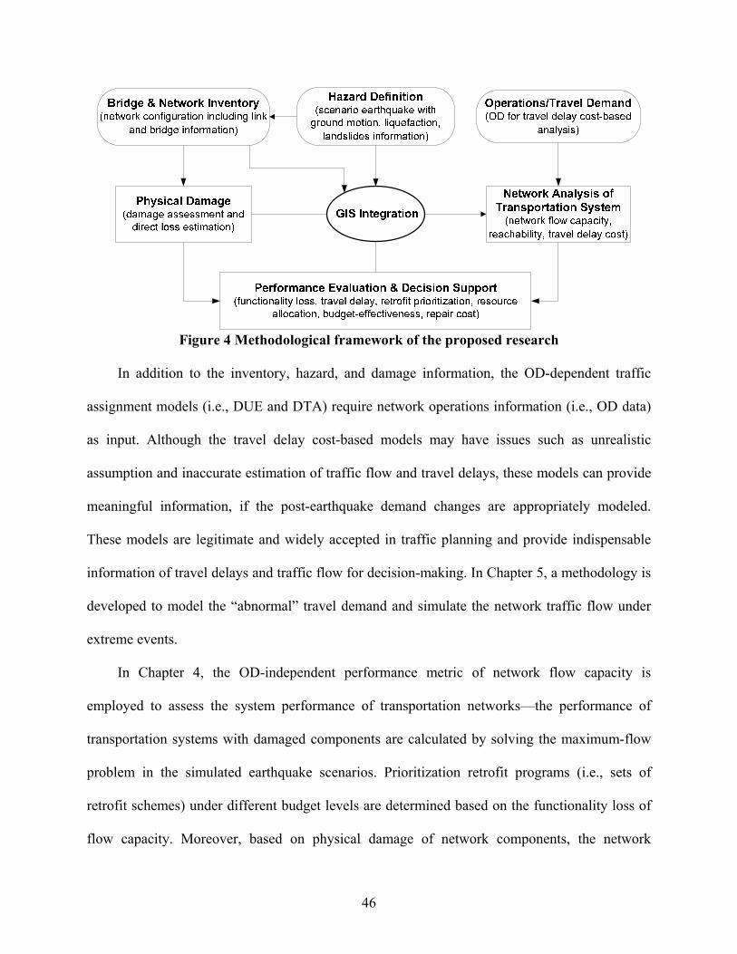
46
Figure 4 Methodological framework of the proposed research
In addition to the inventory, hazard, and damage information, the OD-dependent traffic
assignment models (i.e., DUE and DTA) require network operations information (i.e., OD data)
as input. Although the travel delay cost-based models may have issues such as unrealistic
assumption and inaccurate estimation of traffic flow and travel delays, these models can provide
meaningful information, if the post-earthquake demand changes are appropriately modeled.
These models are legitimate and widely accepted in traffic planning and provide indispensable
information of travel delays and traffic flow for decision-making. In Chapter 5, a methodology is
developed to model the “abnormal” travel demand and simulate the network traffic flow under
extreme events.
In Chapter 4, the OD-independent performance metric of network flow capacity is
employed to assess the system performance of transportation networks—the performance of
transportation systems with damaged components are calculated by solving the maximum-flow
problem in the simulated earthquake scenarios. Prioritization retrofit programs (i.e., sets of
retrofit schemes) under different budget levels are determined based on the functionality loss of
flow capacity. Moreover, based on physical damage of network components, the network
47
reachability of transportation systems can be evaluated by the system connectivity reliability.
The information can be synthesized with direct loss from component damage, traffic flow, travel
delays, etc. to provide decision-making support for disaster management of transportation
infrastructure systems.
3.2 The New Madrid Fault Zone and Hazard Characterization
The target area of this study is the Central United States, which is one of the most
vulnerable regions to seismic hazards in the U.S. This is due to the vicinity of the New Madrid
Seismic Zone (NMSZ), which is roughly located between St. Louis, Missouri and Memphis,
Tennessee. The NMSZ was responsible for the devastating 1811-1812 New Madrid earthquakes,
the largest earthquakes ever recorded in the contiguous United States.
The chance of a moderate earthquake occurring in the NMSZ in the near future is high—
scientists estimate that the probability of a magnitude 6 to 7 earthquake occurring in NMSZ
within the next 50 years is higher than 90% (Hildenbrand et al. 1996). Additionally, most
structures in the NMSZ were not seismically designed, as opposed to those have been in regions
with frequent earthquakes such as California and Japan. To make things worse, earthquake
preparations in the Mid-west region have lagged far behind as compared with other regions, due
to the low frequency high consequence nature of earthquakes in this region. According to a
recent study completed by the MAE Center, a magnitude 7.7 earthquake in the NMSZ could
cause $300 billion direct economic loss, tens of thousands of causalities, and hundreds of
thousands left without homes for the eight central states (Elnashai et al. 2009).
There are three major segments of the primary fault of the NMSZ—the northeast segment,
the Reelfoot Thrust segment, and the southwest segment, as shown in Figure 5 (Cramer 2006).
Such line source representation (on earth’s surface only) is based on the projections of presumed
48
fault planes. The fault planes in the northeast and the southwest segments are assumed vertical,
extending from 5 km to 15 km depth. The thrust segment is a dipping fault and not vertical,
which dips to the southwest at 40 degrees with updip edge at 5 km below the surface and
downdip at 15 km (Schweig 2008; Cramer 2008; Cramer 2006).
A M7.7 earthquake on all the three segments simultaneously is advised by the U.S.
Geological Survey (USGS) as the most appropriate scenario for NMSZ catastrophic earthquake
planning. This “characteristic” earthquake is designed to reflect the historic 1811-1812
earthquakes, in which characteristic means that large earthquake sequences are believed to have
a trend of occurring in approximately the same location with the same magnitude (Elnashai et al.
2009).
The ground motions for the three-rupture M7.7 scenario event are attenuated through rock,
and then propagated through the soil layer above the bedrock. Four sets of ground shaking maps
with 7-10% probability of exceedance in 50 years are developed by the USGS, including PGA
map (see Figure 6), peak ground velocity (PGV) map, spectral acceleration maps of 0.3 second
and 1.0 second.
3.3 Bridge Damage Assessment
Bridges are of primary concern among the major components of the highway transportation
system. Their loss of functionality will have the greatest impact on the system performance to
move people and equipment after the earthquake (CUSEC 2000). The structural damage and
capacity of bridges can be estimated by using fragility curves that define the conditional
exceedance probability of particular limit state (e.g., none damage, slight damage, moderate
damage, extensive damage, and complete damage) for a given ground shaking intensity.
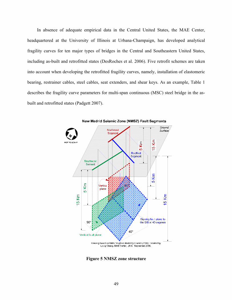
49
In absence of adequate empirical data in the Central United States, the MAE Center,
headquartered at the University of Illinois at Urbana-Champaign, has developed analytical
fragility curves for ten major types of bridges in the Central and Southeastern United States,
including as-built and retrofitted states (DesRoches et al. 2006). Five retrofit schemes are taken
into account when developing the retrofitted fragility curves, namely, installation of elastomeric
bearing, restrainer cables, steel cables, seat extenders, and shear keys. As an example, Table 1
describes the fragility curve parameters for multi-span continuous (MSC) steel bridge in the as-
built and retrofitted states (Padgett 2007).
Figure 5 NMSZ zone structure
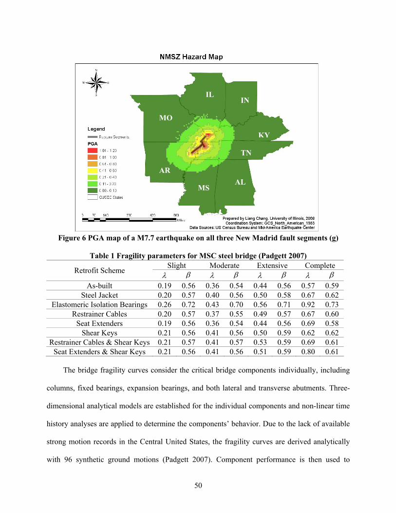
50
Figure 6 PGA map of a M7.7 earthquake on all three New Madrid fault segments (g)
Table 1 Fragility parameters for MSC steel bridge (Padgett 2007)
Slight Moderate Extensive Complete Retrofit Scheme
As-built 0.19 0.56 0.36 0.54 0.44 0.56 0.57 0.59 Steel Jacket 0.20 0.57 0.40 0.56 0.50 0.58 0.67 0.62
Elastomeric Isolation Bearings 0.26 0.72 0.43 0.70 0.56 0.71 0.92 0.73 Restrainer Cables 0.20 0.57 0.37 0.55 0.49 0.57 0.67 0.60
Seat Extenders 0.19 0.56 0.36 0.54 0.44 0.56 0.69 0.58 Shear Keys 0.21 0.56 0.41 0.56 0.50 0.59 0.62 0.62
Restrainer Cables & Shear Keys 0.21 0.57 0.41 0.57 0.53 0.59 0.69 0.61 Seat Extenders & Shear Keys 0.21 0.56 0.41 0.56 0.51 0.59 0.80 0.61
The bridge fragility curves consider the critical bridge components individually, including
columns, fixed bearings, expansion bearings, and both lateral and transverse abutments. Three-
dimensional analytical models are established for the individual components and non-linear time
history analyses are applied to determine the components’ behavior. Due to the lack of available
strong motion records in the Central United States, the fragility curves are derived analytically
with 96 synthetic ground motions (Padgett 2007). Component performance is then used to
IL
MO
AR
MS AL
TN
KY
IN

51
determine the overall performance of the bridge. The capacity of the bridge system is compared
with the demand established by the synthetic records. The combination of regionally appropriate
earthquake records and components-generated fragility curves provide the best available bridge
assessment tool that captures structural performance under probabilistic earthquake impact in the
Central United States (Nielson and DesRoches 2004, 2006a, and 2006b).
Structural fragility is often modeled by a lognormal distribution (Hwang and Jaw 1990;
Shinozuka et al. 2003; Yamazaki et al. 1999). The analytical fragilities developed by the MAE
center can be described as:
lnP( | ) i
ii
aLS PGA a
(3)
where )( is the cumulative density function of the standard normal distribution, a is the
realization of the ground motion intensity, and i and i are the median and dispersion of the
lognormal distribution, respectively, for the i -th limit state of a given structural type (Chang and
Song 2006). The fragility parameters ( i and i ) are related to the structural demand and
capacity, which are essential quantities for analytical fragility curve development. The detailed
procedure of development of the analytical fragility curves from the structural demand and
capacity can be found in Nielson and DesRoches (2004, 2006a, and 2006b).
The MAE Center has proposed five distinct states for bridge damage by ground shaking
(Nielson and DesRoches 2004): None, Slight, Moderate, Extensive, and Complete. As illustrated
in Figure 7, for any given PGA, the probabilities for the bridge to be in any of damage states
( DS ) can be computed from the limit-state exceedance probabilities as follows:
P( ) 1 P( | )DS None Slight PGA (4)
P( ) P( ) P( )DS Slight Slight PGA Moderate PGA (5)
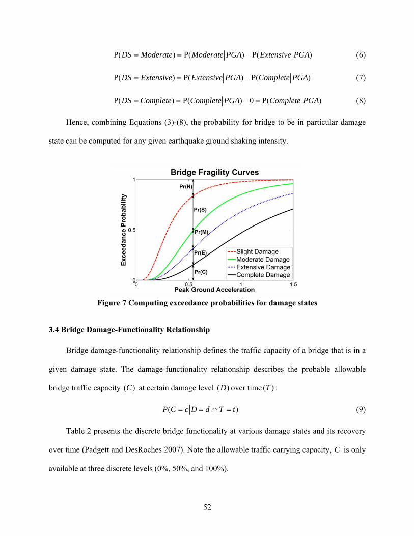
52
P( ) P( ) P( )DS Moderate Moderate PGA Extensive PGA (6)
P( ) P( ) P( )DS Extensive Extensive PGA Complete PGA (7)
P( ) P( ) 0 P( )DS Complete Complete PGA Complete PGA (8)
Hence, combining Equations (3)-(8), the probability for bridge to be in particular damage
state can be computed for any given earthquake ground shaking intensity.
Figure 7 Computing exceedance probabilities for damage states
3.4 Bridge Damage-Functionality Relationship
Bridge damage-functionality relationship defines the traffic capacity of a bridge that is in a
given damage state. The damage-functionality relationship describes the probable allowable
bridge traffic capacity ( )C at certain damage level ( )D over time ( )T :
( )P C c D d T t (9)
Table 2 presents the discrete bridge functionality at various damage states and its recovery
over time (Padgett and DesRoches 2007). Note the allowable traffic carrying capacity, C is only
available at three discrete levels (0%, 50%, and 100%).
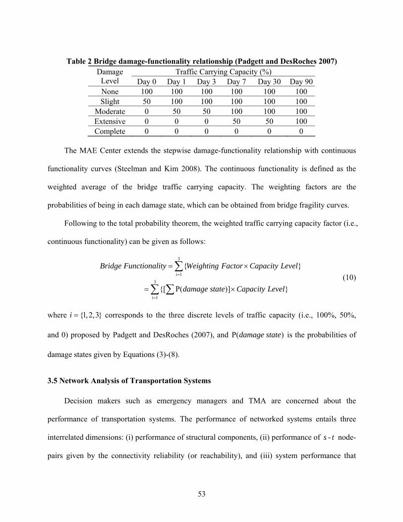
53
Table 2 Bridge damage-functionality relationship (Padgett and DesRoches 2007)
Traffic Carrying Capacity (%) Damage Level Day 0 Day 1 Day 3 Day 7 Day 30 Day 90 None 100 100 100 100 100 100 Slight 50 100 100 100 100 100
Moderate 0 50 50 100 100 100 Extensive 0 0 0 50 50 100 Complete 0 0 0 0 0 0
The MAE Center extends the stepwise damage-functionality relationship with continuous
functionality curves (Steelman and Kim 2008). The continuous functionality is defined as the
weighted average of the bridge traffic carrying capacity. The weighting factors are the
probabilities of being in each damage state, which can be obtained from bridge fragility curves.
Following to the total probability theorem, the weighted traffic carrying capacity factor (i.e.,
continuous functionality) can be given as follows:
3
1
3
1
{ }
{[ P( )] }
i
i
Bridge Functionality Weighting Factor Capacity Level
damage state Capacity Level
(10)
where {1,2,3}i corresponds to the three discrete levels of traffic capacity (i.e., 100%, 50%,
and 0) proposed by Padgett and DesRoches (2007), and P( )damage state is the probabilities of
damage states given by Equations (3)-(8).
3.5 Network Analysis of Transportation Systems
Decision makers such as emergency managers and TMA are concerned about the
performance of transportation systems. The performance of networked systems entails three
interrelated dimensions: (i) performance of structural components, (ii) performance of -s t node-
pairs given by the connectivity reliability (or reachability), and (iii) system performance that
54
measured by the travel delay costs (e.g., the total system travel time). The first dimension has
been discussed in Sections 3.2, 3.3 and 3.4. In Section 3.5, the scope of network analysis
presented is limited to the latter two dimensions.
3.5.1 Network Flow Capacity
The network flow capacity is an intrinsic property of the network, which is a suitable
performance metric of emergency flow capacity of a transportation network in immediate
population evacuation scenarios. Maximum flow is a measure of the network flow capacity of a
transportation network, which is an essential ingredient in evaluating the system serviceability
when the road network’s damage state can be specifically determined (Fenves and Law 1979). In
transportation engineering, the network flow capacity is often defined in the unit of vehicles per
hour (vph).
Maximum flow is the largest possible total flow between the source nodes and sink nodes
without exceeding the capacity of any edge (Ahuja et al. 1993). For a capacitated network
( , )G N A with nonnegative capacity iju associated with arc ( , )i j A , the maximum flow
between the source node s and the sink node t (or the network flow capacity) that satisfies the
arc capacities and mass balance constrains can be defined as:
Maximize (11)
subject to
{ :( , ) } { :( , ) }
for
0 for all { and }
forij ji
j i j A j i j A
i = s
x x i N s t
i = t
(12)
0 for each ( , )ij ijx u i j A (13)
55
where ijx is the flow on arc ( , )i j . Equation (12) is the mass balance constraint for each node in
the node set N . Equation (13) defines the capacity constraint for each link in the arc set A .
The formulation described above is a standard maximum flow problem, which can be
solved by several well-established algorithms such as the Ford-Fulkerson algorithm and the
Edmonds-Karp algorithm. However, the network seismic retrofit problem at hand deals with the
retrofit of a subset of bridges to improve the system performance with additional constraints such
as limited retrofit funding and variable capacity constraints, which falls into the category of the
NDP. Network design is a term for network optimization, and sometimes deals with the addition
of new road intersections (nodes) or segments (links) or lanes to an existing network to achieve a
certain system performance goal. The NDP problem is known as NP-hard and difficult to solve
using classic algorithms. In this study, a network flow capacity-based NDP are formulated to
solve the seismic retrofit prioritization problem. The detailed mathematical formulation and
solution methods are presented in Chapter 4.
3.5.2 Reliability of Network Reachability
Reliability of network reachability, or the probability of connectivity between node-pairs
can be assessed by using graph theory. This study employs an analytical system reliability
approach following the RDA, which is developed based on disjoint minimal path algorithms.
For a given network G , when it has at least one path between a particular node-pair, the
structure function of the network is defined as 1, otherwise 0. The structure function for the
network that has at lease one path from the source to the sink can be written as (Li and He 2002):
1
( )K
kk
G A
(14)
56
where kA is the k -th shortest path of the network, and K is the total number of shortest paths.
By recursively decomposing an arbitrary shortest path of the network until there exists no
connected sub-graphs, the structure function of the network can be given by:
1 2
1 1,
11 1 2 1
( )c c nc
c n c
m m mN N
i i i i i i i i ii i i i m i m
G L c A A c A c A c A
(15)
where iL is the i -th disjoint shortest path, N is the total number of disjoint shortest paths, ic is
the i -th recursive coefficient with Boolean simplification, ,i cm is the total number of connected
sub-graphs of the sub-graph iG , and iG is a sub-graph obtained by deleting the component
1ia A from the original network G .
When paths between the source and terminal are found in the sub-graphs, they are disjoint
link sets by nature according to the De Morgan’s Rule and thus contribute to the network
reliability; for those sub-graphs containing no paths between the node-pair, they are disjoint cut
sets and contribute to system failure probability (He and Li 2001; Li and He 2002). When
disjoint cut sets or link sets, ,iS setNi ,...,1 are identified, the system failure probability or
reliability ( )sysP E is computed by summing up the results
1
( ) ( )setN
sys ii
P E P S
(16)
The RDA can be applied to all types of infrastructure networks regardless the network size
or the topology. The RDA can efficiently compute reliability or failure probability—it can either
give exact network reliability or give an approximate reliability bound with controllable
precision when it is not plausible to find all paths in extremely complex and large infrastructure
networks (Li and He 2002).
57
3.5.3 Travel Delay Cost Metric
The travel delay cost metrics are highly dependent on detailed OD demand information.
After a disruptive event such as a major earthquake, the travel behavior (i.e., route choices) and
travel demand could change significantly due to travelers’ reaction to bridge damage, road
closures, and congestions. The conventional demand model (i.e., fixed demand model) has been
proved unsuitable for post-earthquake traffic modeling and may give inaccurate estimate of
travel delay cost.
Though it is still infeasible to obtain realistic behavior of traveler route choice and “real-
time” travel demand, post-earthquake travel demand can be approximated with some general
principles to capture the essential characteristics of post-earthquake travel patterns and effects of
emergency facilities such as hospitals and emergency shelters. The approximated post-
earthquake travel demand can then be loaded to the damaged transportation networks to predict
corresponding traffic flow on the road network with static or dynamic traffic simulation models.
Note the proposed methodology does not aim to provide “real-time” post-earthquake traffic
simulation, but rather to provide some general principles and procedures for emergency training
or planning purposes.
In this study, several travel delay cost metrics are used to measure the post-earthquake
performance of transportation systems, including the commonly used total system travel time
and the OD route travel time. Such system performance metrics can be given by static or
dynamic traffic assignment models.
The static model gives steady state traffic flow in UE (Wardrop 1952; Sheffi 1985). The
mathematical formulation of UE may be expressed as:
58
0
min ( ) ( )dix
ii
Z x t (17)
with definitional constrains , ,rs rsi k i k
r s k
x f i
subject to , ,
0, ,
rsk rs
k
rsk
f q r s
f r s
where ix is the traffic flow on arc i , arc seti A ; it is the travel time on link i ; rskf is the
traffic flow on the -thk path connecting OD pair -r s ; ,rsi k is the indictor variable: , 1rs
i k if road
segment i is part of the -thk route from r (origin) to s (destination), otherwise , 0rsa k .
For static traffic assignment models, the total system travel time can be written as:
0( ) (1 [ ] )ii i i i
i i i
xTSTT x t x x t
C (18)
where 0t is the free-flow travel time, iC is the traffic carrying capacity of link i , and are
variable parameters of the link performance function (also known as the travel delay function).
In contrast to the static models, the dynamic models do not depend upon the link
performance functions, but use cell transmission model (CTM), in which a link is divided into
several cell and the congestion on at cells determines the link travel time. The congestion on a
link is time-dependent and can propagate to other links, which is more realistic to represent the
spillback effect on road networks. For dynamic models, the total system travel time (TSTT) can
be written as:
( )E Di i
i
TSTT t t (19)
59
where Eit is the vehicle exit time of link i ; D
it is the vehicle departure time of link i . The TSTT
tends to increase as the travel demand increases and the link capacity degrades for both the static
and dynamic assignment models.
OD path cost is the total travel cost on the link segments of the shortest paths (in terms of
travel time) between the origin and destination node-pairs. The OD path cost gives a more
specific measure of the performance of the routes between interested origins and destinations,
while the TSTT provides a good overall measure of the system performance.
Chapter 5 describes a methodology to model the “abnormal” post-earthquake travel demand
and simulate the corresponding network traffic flow with the DUE and DTA. The major
assumptions are presented in Chapter 5 and the key procedures of the proposed methodology are
illustrated by case studies.
60
CHAPTER IV OD-INDEPENDENT PERFORMANCE EVALUATION AND SEISMIC
RETROFIT PROGRAM PLANNING
Aiming at assessing the system performance of transportation networks under extreme
events and providing decision support for disaster management of transportation infrastructures,
this section adapts the NBSR framework proposed by Kim and colleagues (2008) and extends
the framework with the OD-independent performance metrics discussed in Section 3.5, i.e., the
metrics of network flow capacity and reachability.
This chapter focuses on the evaluation of transportation systems and seismic retrofit
program planning with the OD-independent performance metrics. The modeling of post-
earthquake travel demand and performance evaluation of transportation systems with travel
delay cost metrics are discussed in Chapter 5.
In the following sections, first the network flow capacity-based formulation and the
solution algorithms are presented in Section 4.1. The convergence of MCS and the parameter
sensitivity are tested and the proposed methodology is demonstrated with the road network in the
Memphis metropolitan area. Next, Section 4.2 presents the application of the RDA for network
reachability and quantifies the connectivity reliability between the safe zones and evacuation
zones for the Memphis road network. Lastly, Section 4.3 summarizes the major conclusions.
4.1 Network Flow Capacity-based NBSR
This section presents the mathematical formulation and solution algorithms for the network
capacity-based NBSR. The convergence of MCS and the sensitivity to input parameters are
tested with the Sioux-Falls benchmark network. This extended NBSR methodology for bridge
61
retrofit prioritization and resource allocation is demonstrated with a real-world case study in
Section 4.1.7.
4.1.1 Mathematical Framework
In the extended NBSR framework, the road network is represented by an undirected graph
( , )G N A , where N is the node set and A is the link set. Each link ( , )i j A has a capacity of
iju . Let NNO be the set of source nodes representing the evacuation zones, and DN N be
the set of sink nodes representing the safe zones. Let z be the total evacuation flow from ON to
DN after a certain earthquake scenario. The objective of our model is to maximize the expected
value of z .
Let B A be the set of the links with a bridge. Denote ( , ) {0,1,2, }K i j as the set of
indices of mutually exclusive retrofit alternatives for bridge ( , )i j B . ( , )K i j always contains
the “do-nothing” alternative, i.e., retrofit scheme 0. If two retrofit schemes can be applied
together, the combined use of these two schemes should be considered as a third scheme,
because retrofit effectiveness is usually not additive. Let {0,1}kijy be the retrofit project
variable, where 1kijy if retrofit scheme k is applied to bridge ( , )i j (i.e., which is denoted as
project ( , )i j k ), or 0 otherwise. Then kijyy defines a retrofit program.
Let iju be the residual capacity of bridge ( , )i j B after earthquake. Given the network
( , )G N A and iju ), ijuu is only related to both retrofit program y and some random
variables ξ representing uncertainties (e.g., the earthquake intensity at a bridge location and the
damage incurred to a bridge), and could be written as ( , )u y ξ . z is only related to the post-
earthquake capacity of the bridges and could be written as ( , )z zu u y ξ . Therefore, the

62
objective of our model can be written as max E ( , )z ξy
u y ξ , and the optimal retrofit program is
* arg max E ( , )z ξy
y u y ξ , where operator Eξ is to take expectation with regard to ξ .
For any given ξ , an integer programming problem must be solved to obtain the value of
( , )z u y ξ . Therefore, it is extremely challenging to calculate max E ( , )z ξy
u y ξ when ξ is
continuous and/or contains a large number of random variables. In traditional scenario-based
stochastic programming methods, the uncertainty is represented by a small number of scenarios
with the realization of ξ , sξ , 1,...,s S , and each scenario happens with probability sp (Liu et
al. 2009). Then the objective of the problem reduces to 1
max ( , )S
s ss
p z
yu y ξ , while the optimal
retrofit program is *
1
arg max ( , )S
s ss
p z
y
y u y ξ . Because it is usually time-consuming to solve
such stochastic programming problems, this approach is suitable only when S is small.
In the present study, a simple scenario-based sampling and ranking procedure is proposed
to determine the retrofit program. First, a large number of scenarios are generated using the
simulation approach. For each scenario s , the optimum retrofit program is obtained as
* arg max ( , )s szy
y u y ξ . Then e , the effectiveness indicator of the retrofit projects (a vector of
non-negative integers), is calculated based on these *sy (a vector of binary numbers) as follows:
*
1 1
1( ) arg max ( , )
S S
s s ss s
p zS
y
e e y e u y ξ (20)
where *( )se y is the effectiveness function of projects in a single scenario. The second equality in
(20) holds because each simulated scenario is assumed to occur with equal probability 1
spS
.
63
The advantages of this method are: (i) the total number of scenarios could be much larger
than what the stochastic programming method can handle, and (ii) the effectiveness indicators e
could be easily combined with other types of cost-effectiveness measurements in the cost-
effectiveness analysis to obtain the final retrofit program. It shall be noted that the proposed
sampling and ranking procedure is not an exact method, but it is sufficiently simple and efficient
for large-scale applications.
The proposed methodology framework is illustrated in Figure 8. For a given representative
earthquake event, Monte Carlo simulation is used to generate multiple earthquake intensity
scenarios (i.e., earthquake intensity at each bridge location). For each earthquake intensity
scenario, a second round of simulation is used to generate the damage state scenarios (i.e., the
damage state of each bridge) based on the structural characteristics of bridges (i.e., the fragility
curves, Nielson and DesRoches 2004). The damage state scenarios are converted to post-
earthquake residual capacity scenarios ( , )su y ξ based on the bridge damage-functionality
relationship (Padgett and DesRoches 2007). A NDP model is run for each scenario sξ to
calculate e from Equation (20). The cost-effectiveness analysis method is then applied to
determine the final retrofit program. The expected effectiveness of the retrofit program is
obtained by running a maximum flow problem (MFP) model in another set of sampled scenarios.
The major components of this framework are explained in detail in the following sections.
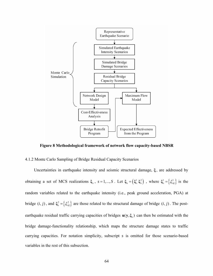
64
Figure 8 Methodological framework of network flow capacity-based NBSR
4.1.2 Monte Carlo Sampling of Bridge Residual Capacity Scenarios
Uncertainties in earthquake intensity and seismic structural damage, ξ , are addressed by
obtaining a set of MCS realizations sξ , 1,...,s S . Let 1 2s s sξ ξ ξ , where 1 1
s sijξ is the
random variables related to the earthquake intensity (i.e., peak ground acceleration, PGA) at
bridge ( , )i j , and 2 2s sijξ are those related to the structural damage of bridge ( , )i j . The post-
earthquake residual traffic carrying capacities of bridges ( , )su y ξ can then be estimated with the
bridge damage-functionality relationship, which maps the structure damage states to traffic
carrying capacities. For notation simplicity, subscript s is omitted for those scenario-based
variables in the rest of this subsection.
65
4.1.2.1 Ground Intensity
Based on a representative earthquake event, PGAij , the median of the earthquake intensity
at the location of bridge ( , )i j , can be predicted by the ground motion models (also known as an
attenuation relationship), where the probability of a ground motion exceeding a particular
threshold value is modeled with the Poisson model (Cornell 1968; Zhang et al. 2004).
In every simulated scenario, the uncertainty of PGA 1ij is first generated by MCS, and then
the simulated earthquake intensity PGAij is calculated based on PGAij and 1ij . 1
ij is often
assumed to follow a lognormal distribution (Boore 2003; Campbell 1985; Dueñas-Osorio and
Vemuru 2009), since the seismic ground motions are estimated with empirical attenuation
relationships that are usually modeled as the product of a function of magnitude, distance, site
classification, and fault rupture mechanism, etc. The logarithm of PGA at the location of
bridge ( , )i j , ln(PGA )ij , then follows a normal distribution and can be written as:
1ln PGA ln(PGA )ijij ij (21)
PGAij is calculated by assuming a coefficient of variation (c.o.v.) of 0.6 for the lognormal
distribution of PGA (Adachi and Ellingwood 2007).
4.1.2.2 Bridge Fragility and Seismic Damage
The sampling of earthquake intensities is followed by the determination of structural
damage states. With the obtained PGAij from the previous step, kijD , the structural damage level
of bridge ( , )i j under retrofit type k , can be calculated with a sampled random variable 2ij in
conjunction with the structural fragility curves:
1 2( ( ), )k kij ij ij ij ijD D PGA (22)
66
where 2ij represents the uncertainty of structural damage in the fragility curves of bridge ( , )i j .
4.1.2.3 Bridge Damage-Functionality Relationship
The bridge damage-functionality relationship is employed to propagate the uncertainties in
ground intensity and structural damage to the residual traffic-carrying capacity. Such relationship
defines kiju , the residual capacity of bridge ( , )i j when applying retrofit type k , based on the
bridge damage state kijD ; i.e.
1 2 1 2,( ), ( , )k k k k
ij ij ij ij ij ij ij ij iju u D PGA u (23)
For demonstration purposes, the cross-sectional capacity values on Day-3 are taken as the
corresponding traffic carrying capacity hereinafter, since the scope of evacuation is limited to
short-term steady-state flow. Although the allowable traffic carrying capacity is only available at
three discrete levels, for regions with low-probability-high-consequence seismic risks, e.g., the
Central United States, the scarcity of data mandates that the damage-functionality relationship
proposed by Padgett and DesRoches (2007) be utilized.
With the bridge fragility curves and the damage-functionality relationship, the performance
of bridges can be linked to earthquake intensity. The residual capacities of bridges can then be
used to determine the capacities of corresponding links in the network.
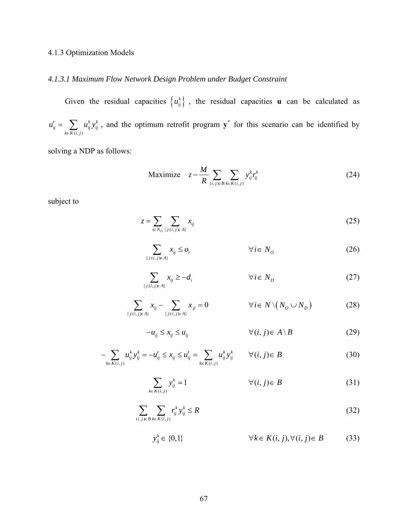
67
4.1.3 Optimization Models
4.1.3.1 Maximum Flow Network Design Problem under Budget Constraint
Given the residual capacities kiju , the residual capacities u can be calculated as
( , )
k kij ij ij
k K i j
u u y
, and the optimum retrofit program *y for this scenario can be identified by
solving a NDP as follows:
( , ) ( , )
Maximize k kij ij
i j B k K i j
Mz y r
R
(24)
subject to
{ :( , ) }O
iji N j i j A
z x
(25)
{ :( , ) }
ij ij i j A
x o
Oi N (26)
{ :( , ) }
ij ij i j A
x d
Di N (27)
{ :( , ) } { :( , ) }
0ij jij i j A j i j A
x x
\ O Di N N N (28)
ij ij iju x u ( , ) \i j A B (29)
( , ) ( , )
k k k kij ij ij ij ij ij ij
k K i j k K i j
u y u x u u y
( , )i j B (30)
( , )
1kij
k K i j
y
( , )i j B (31)
( , ) ( , )
k kij ij
i j B k K i j
r y R
(32)
{0,1}kijy ( , ), ( , )k K i j i j B (33)

68
where M is a non-negative constant indicating the numerical tolerance of flow values, ijx is the
evacuation flow on link ( , )i j , io and id are respectively the maximum evacuation flows which
the evacuation/safe zone i can generate or receive, kijr is the cost of retrofit scheme k for bridge
( , )i j , and R is the total budget.
Objective function (24) not only maximizes the total evacuation flow z but also minimizes
the adjusted total retrofit cost, ( , ) ( , )
k kij ij
i j B k K i j
My r
R . Including this cost term in the objective
function ensures that the program will use the smallest expenditure to achieve the maximum
evacuation flow, especially in low-damage scenarios where R exceeds the actual retrofit needs.
In light of (32), ( , ) ( , )
k kij ij
i j B k K i j
My r M
R
, and hence minimizing the retrofit costs does not
compromise the maximum flow z by more than the tolerance value M .
Constraint (25) defines z as the total flow evacuated from the evacuation zones.
Constraints (26)-(28) are the flow conservation constraints at each node. Constraints (29) and
(30) are respectively the capacity constraints for links without and with bridges. It is assumed
that reverse traffic is allowed for earthquake rescue and relief so the capacities for positive and
negative flows are equal. If the assumption does not hold, these constraints can be modified by
using different values of iju for the left-hand side and the right-hand side. Constraint (31)
ensures that exactly one retrofit scheme (including “do-nothing”) is applied to any bridge.
Constraint (32) is the budget constraint. Constraint (33) defines the binary variables.
NDP can be solved by commercial integer programming (IP) solvers such as ILOG
CPLEX®, especially when the problem size is small or moderate. It can also be solved with

69
various heuristic algorithms such as greedy heuristic and Lagrangian relaxation (Fisher 1981).
The following subsection presents a LR-based solution algorithm.
4.1.3.2 Lagrangian Relaxation (LR) Solution Algorithm
First the budget constraint (32) and the bridge capacity constraint (30) are relaxed, with R ,
ij , ij being the Lagrangian multipliers of (32), the right-hand part of (30) (i.e.,
( , )
k kij ij ij
k K i j
x u y
), and the left-hand part of (30) (i.e., ( , )
k kij ij ij
k K i j
u y x
), respectively. Adding
the corresponding penalty terms to the objective function (24) yields the following relaxed
problem:
( , ) ( , ) ( , ) ( , )
( , ) ( , ) ( , ) ( , )
Maximize ( ) k k k kij ij R ij ij
i j B k K i j i j B k K i j
k k k kij ij ij ij ij ij ij ij
i j B k K i j i j B k K i j
ML z r y R r y
R
u y x u y x
(34)
subject to
(25)-(28), (31) and (33),
( , )ij ij iju x u i j A (35)
where constraints (35) replace (29) for computational efficiency.
The objective function (34) can be rearranged and written as:
( , ) ( , )
( , )
Maximize ( )
( ) ( )
( )
R
k k kij ij ij R ij ij
i j B k K i j
ij ij iji j B
L R
Mu r y
R
z x
(36)

70
For any set of multipliers { } { } { }R ij ij , the relaxed problem is separable. First of
all, the first term RR is a constant. The second term ( , ) ( , )
( ) k k kij ij ij R ij ij
i j B k K i j
u r y
only
contains the variable kijy and constraints (31) and (33). Because k
ijy of different k are mutually
exclusive for any bridge ( , )i j , its value can be determined by the following equation:
( , )
( , ) ( , ) ( , )
max ( ) max ( )k k k k kij ij ij R ij ij ij ij ij R ij
k K i ji j B k K i j i j B
u r y u r
(37)
which can be solved by enumerating all elements in ( , )K i j . The third term ( , )
( )ij ij iji j B
z x
only contains variable ijx and z , and is a minimum cost flow problem with flow conservation
constraints (25)-(28) and capacity constraint (35). Such problem can be solved within
polynomial time (e.g., ( log )( log )O A N A N N as proposed by Orlin (1988). Therefore,
given any set of , the relaxed problem has the same computational complexity as a minimum
cost network flow problem and can be solved in polynomial time. The Lagrangian dual (LD)
min ( )L L
, which serves as an upper bound of the original NDP, can be solved efficiently by
iteratively solving the relaxed problem and updating the value of with methods such as the
subgradient method (Fisher 1981).
In every iteration, a heuristic feasible solution could also be obtained. ( ) kij ij iju can be
considered as the effectiveness of project ( , )i j k , incurring cost kijr . Given the budget R ,
various cost-effectiveness analysis methods (as described in the next section) can be applied to
identify the retrofit program y (Patidar et al. 2007). The maximum evacuation flow achieved by
retrofit program y is a lower bound of the original optimal flow. This lower bound can be solved

71
as a maximum flow problem*. The difference between the lower bound and the upper bound is
the optimality gap, which is the maximum possible difference between the current feasible
solution and the real optimum.
The LR method does not always yield an exact optimum solution, especially when the scale
of the problem is large. If needed, the LR algorithm can be incorporated into a branch and bound
framework (Ahuja et al. 1993) to reduce the optimality gap. However, as shown in the next
section, the solution for each scenario is only used as an estimation of the effectiveness of
projects, and hence obtaining the exact optimality is not ultimately important.
4.1.4 Effectiveness Measurement and Project Selection
The solutions to NDP for all S scenarios are used to compute the effectiveness of projects,
kijee from (20). The elements in function *( )se y are defined as:
:
, ( , ) , ( , ) \ 0k kij ij
k k kij ij ij
k u u
e r y i j B k K i j
, (38)
where kije is the effectiveness of project ( , )i j k in a single scenario, and the projects with 0k
(the “do-nothing” benchmarks) are not included in the computation. The effectiveness, kije , is
calculated as the average value of all kije across all scenarios.
In light of the project mutually exclusive constraints (31), it can be seen from (38) that in a
certain scenario, k k k kij ij ij ije r y r if project ( , )i j k is selected by NDP, i.e., 1k
ijy . This is based
on the assumption that if a project is selected, it shall at least provide a relative effectiveness
measure comparable to its cost; i.e., kijy is conceptually analogous to an effectiveness/cost ratio.
* When y is fixed, the NDP model reduces to a maximum flow model (with decision variables x and (24)-(30)), which calculates the maximum evacuation flow under retrofit program y . This problem can be solved by standard
network flow algorithms in polynomial time (e.g., Edmonds and Karp 1972).
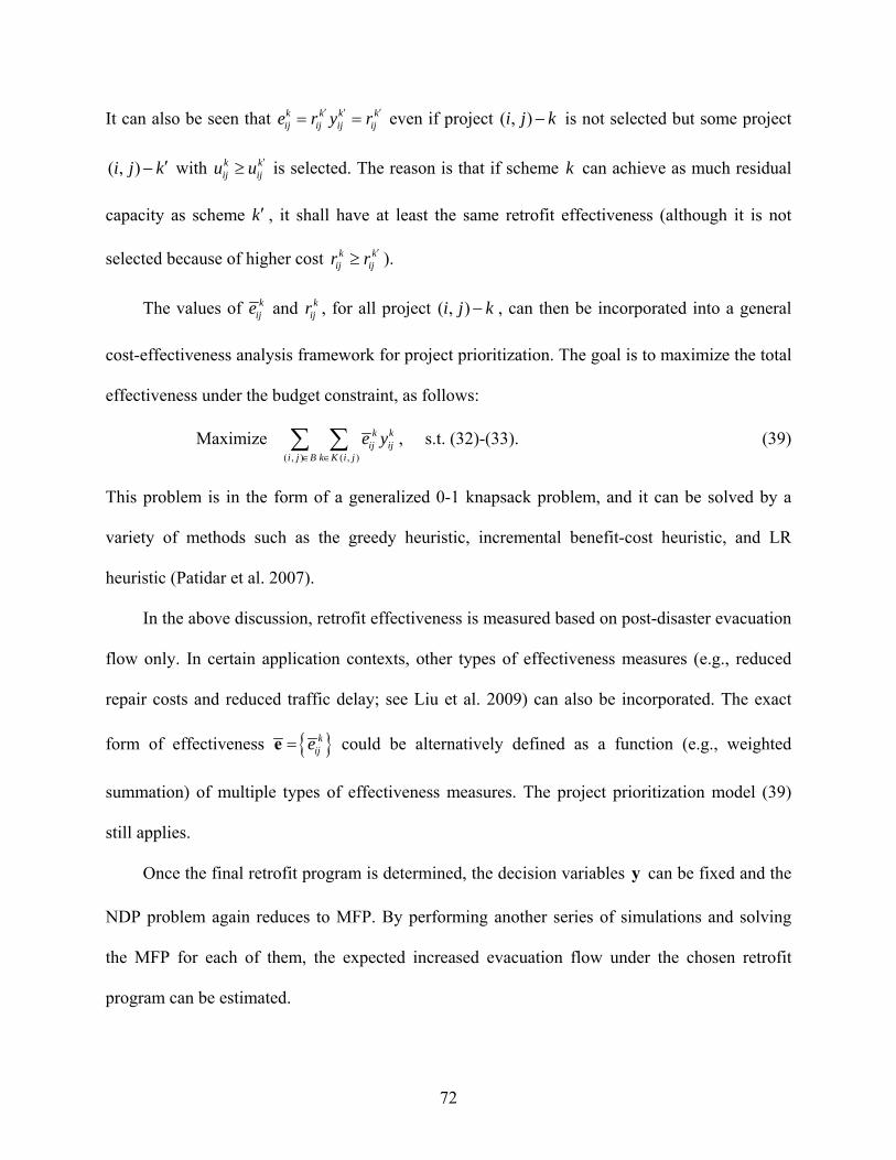
72
It can also be seen that k k k kij ij ij ije r y r even if project ( , )i j k is not selected but some project
( , )i j k with k kij iju u is selected. The reason is that if scheme k can achieve as much residual
capacity as scheme k , it shall have at least the same retrofit effectiveness (although it is not
selected because of higher cost k kij ijr r ).
The values of kije and k
ijr , for all project ( , )i j k , can then be incorporated into a general
cost-effectiveness analysis framework for project prioritization. The goal is to maximize the total
effectiveness under the budget constraint, as follows:
( , ) ( , )
Maximize k kij ij
i j B k K i j
e y , s.t. (32)-(33). (39)
This problem is in the form of a generalized 0-1 knapsack problem, and it can be solved by a
variety of methods such as the greedy heuristic, incremental benefit-cost heuristic, and LR
heuristic (Patidar et al. 2007).
In the above discussion, retrofit effectiveness is measured based on post-disaster evacuation
flow only. In certain application contexts, other types of effectiveness measures (e.g., reduced
repair costs and reduced traffic delay; see Liu et al. 2009) can also be incorporated. The exact
form of effectiveness kijee could be alternatively defined as a function (e.g., weighted
summation) of multiple types of effectiveness measures. The project prioritization model (39)
still applies.
Once the final retrofit program is determined, the decision variables y can be fixed and the
NDP problem again reduces to MFP. By performing another series of simulations and solving
the MFP for each of them, the expected increased evacuation flow under the chosen retrofit
program can be estimated.

73
4.1.5 Convergence Tests
This section discusses the convergence of the network-flow capacity algorithms. The
Sioux-Falls network, one of the widely used benchmark networks in transportation engineering,
is assumed to have only ten bridges so the proposed algorithms can be investigated. The Sioux-
Falls network consists of 24 nodes and 76 edges, as shown in Figure 9. Nodes 1, 2, and 3
(illustrated by red circles in Figure 9) are assumed to be the seriously impacted area or
evacuation zones, and nodes 7, 18, 19, 20, and 21 as the safe zones (marked by green circles in
Figure 9). The network has 10 bidirectional bridges and the detailed bridge information is
described in Table 1, including the node numbers that indicate the location of each bridge, the
structure type, length, and PGA level, etc. These bridges are susceptible to earthquake and
limited resource shall be allocated to mitigate potential functional losses by retrofitting these
bridges. Road capacities are converted from the damage states of bridges according to the bridge
fragilities and bridge functionality relationships, as described in Chapter 3.
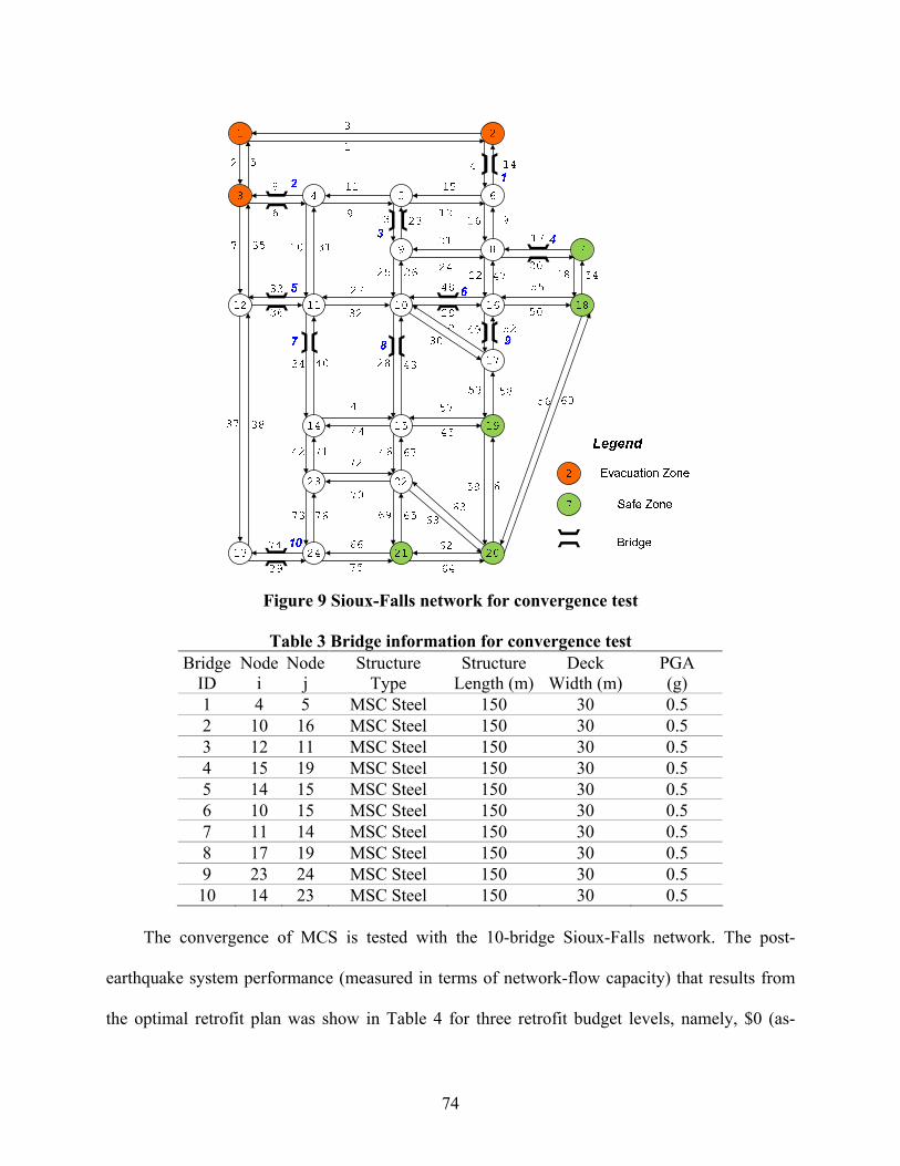
74
Figure 9 Sioux-Falls network for convergence test
Table 3 Bridge information for convergence test
Bridge ID
Node i
Node j
Structure Type
Structure Length (m)
Deck Width (m)
PGA (g)
1 4 5 MSC Steel 150 30 0.5 2 10 16 MSC Steel 150 30 0.5 3 12 11 MSC Steel 150 30 0.5 4 15 19 MSC Steel 150 30 0.5 5 14 15 MSC Steel 150 30 0.5 6 10 15 MSC Steel 150 30 0.5 7 11 14 MSC Steel 150 30 0.5 8 17 19 MSC Steel 150 30 0.5 9 23 24 MSC Steel 150 30 0.5 10 14 23 MSC Steel 150 30 0.5
The convergence of MCS is tested with the 10-bridge Sioux-Falls network. The post-
earthquake system performance (measured in terms of network-flow capacity) that results from
the optimal retrofit plan was show in Table 4 for three retrofit budget levels, namely, $0 (as-
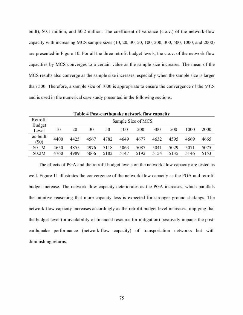
75
built), $0.1 million, and $0.2 million. The coefficient of variance (c.o.v.) of the network-flow
capacity with increasing MCS sample sizes (10, 20, 30, 50, 100, 200, 300, 500, 1000, and 2000)
are presented in Figure 10. For all the three retrofit budget levels, the c.o.v. of the network flow
capacities by MCS converges to a certain value as the sample size increases. The mean of the
MCS results also converge as the sample size increases, especially when the sample size is larger
than 500. Therefore, a sample size of 1000 is appropriate to ensure the convergence of the MCS
and is used in the numerical case study presented in the following sections.
Table 4 Post-earthquake network flow capacity
Sample Size of MCS Retrofit Budget Level 10 20 30 50 100 200 300 500 1000 2000
as-built ($0)
4400 4425 4567 4782 4649 4677 4632 4595 4669 4665
$0.1M 4650 4855 4976 5118 5063 5087 5041 5029 5071 5075 $0.2M 4760 4989 5066 5182 5147 5192 5154 5135 5146 5153
The effects of PGA and the retrofit budget levels on the network-flow capacity are tested as
well. Figure 11 illustrates the convergence of the network-flow capacity as the PGA and retrofit
budget increase. The network-flow capacity deteriorates as the PGA increases, which parallels
the intuitive reasoning that more capacity loss is expected for stronger ground shakings. The
network-flow capacity increases accordingly as the retrofit budget level increases, implying that
the budget level (or availability of financial resource for mitigation) positively impacts the post-
earthquake performance (network-flow capacity) of transportation networks but with
diminishing returns.
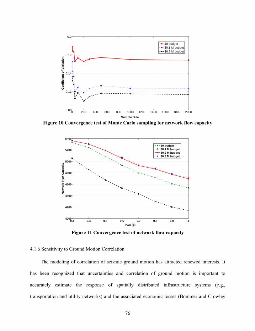
76
0 200 400 600 800 1000 1200 1400 1600 1800 20000.08
0.11
0.14
0.17
0.2
Sample Size
Co
effi
cien
t o
f V
aria
tio
n
$0 budget$0.1 M budget$0.2 M budget
Figure 10 Convergence test of Monte Carlo sampling for network flow capacity
0.3 0.4 0.5 0.6 0.7 0.8 0.9 14000
4200
4400
4600
4800
5000
5200
5400
PGA (g)
Net
wo
rk F
low
Cap
acit
y
$0 budget$0.1 M budget$0.2 M budget$0.3 M budget
Figure 11 Convergence test of network flow capacity
4.1.6 Sensitivity to Ground Motion Correlation
The modeling of correlation of seismic ground motion has attracted renewed interests. It
has been recognized that uncertainties and correlation of ground motion is important to
accurately estimate the response of spatially distributed infrastructure systems (e.g.,
transportation and utility networks) and the associated economic losses (Bommer and Crowley
77
2006; Adachi and Ellingwood 2007; Lee and Kiremidjian 2007; Park et al. 2007; Zerva 2008).
The physical causes of spatial variation include: (i) the wave passage effect, (ii) extended source
effect, (iii) scattering effect (or ray path effect), and (iv) the attenuation effects (Zerva 2008).
Although the spatial variability has been accounted for extended structures (e.g., bridges)
(Burdette et al. 2008; Burdette and Elnashai 2008; Sextos, Pitilakis, and Kappos 2003), the
uncertainties of ground motion prediction in lifeline earthquake engineering are often
disregarded in deterministic seismic risk analysis, in which only the medians of ground motion
were used to obtain the best estimate or the mean value of risk (Zhou 2006). Additionally, the
spatial dependence of the site-to-site ground motions has not been extensively investigated (Park
et al. 2007) and majorly done with Monte Carlo simulations (Park et al. 2007; Bommer and
Crowley 2006).
This section discusses the effects of ground motion correlation and uncertainties on the
performance of transportation systems. The detailed procedures for generating seismic motions
that incorporate uncertainties and spatial correlation are described in Appendix C. In this analysis,
a magnitude 8.0 event on a hypothetical Sioux Falls vertical rupture plane is used for illustrative
purposes. The next generation attenuation (NGA) relationship by Campbell and Bozorgnia (2007)
is used to determine the distribution of median ground motion intensity (e.g., PGA) at each site
on the Sioux-Falls road network (Figure 12).
The effects of uncertainty and correlation of ground motions on the response of spatially
distributed infrastructure systems are studied in the 10 cases listed in Table 5. The first case
(Case I) does not consider the inter-event ( 1 0 ) or intra-event ( 2 0 ) and only uses the
median PGAs when generating the spatial distribution of ground motions. The ground motions in
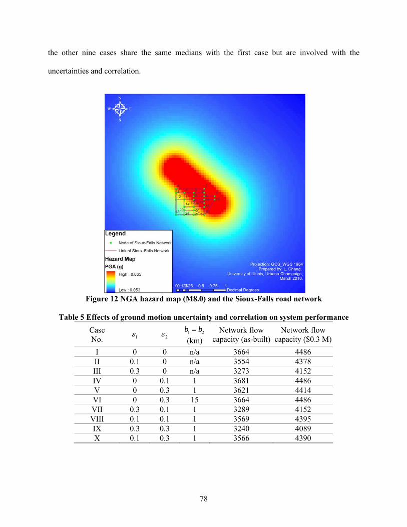
78
the other nine cases share the same medians with the first case but are involved with the
uncertainties and correlation.
Figure 12 NGA hazard map (M8.0) and the Sioux-Falls road network
Table 5 Effects of ground motion uncertainty and correlation on system performance
Case No. 1 2 1 2b b
(km) Network flow
capacity (as-built)Network flow
capacity ($0.3 M)
I 0 0 n/a 3664 4486 II 0.1 0 n/a 3554 4378 III 0.3 0 n/a 3273 4152 IV 0 0.1 1 3681 4486 V 0 0.3 1 3621 4414 VI 0 0.3 15 3664 4486 VII 0.3 0.1 1 3289 4152 VIII 0.1 0.1 1 3569 4395 IX 0.3 0.3 1 3240 4089 X 0.1 0.3 1 3566 4390
79
Cases II and III assume no intra-event uncertainty ( 2 0 ) and only consider the inter-
event uncertainties ( 1 0.1 and 0.3 , respectively). The performance of transportation systems
(i.e., network flow capacity) tends to decrease as 1 increases.
Cases IV, V and VI assume no inter-event uncertainty ( 1 0 ) and focus on the intra-event
uncertainties. The simulation results show that the effect of intra-event uncertainty is not
significant—the performance of network flow capacity deteriorates slightly when increasing the
intra-event uncertainty and the correlation length. In fact, the effect of intra-event uncertainty is
trivial (about 1.6%) on the system performance, as illustrated in the Cases IV and V. Since
shorter correlation distance tends to represent the actual case more closely (Shinozuka et al. 2005;
Zhou 2006), a relatively small correlation distance ( 1 2 1b b km) is used in the other cases
when considering the intra-event uncertainty.
Both inter- and intra-event uncertainties are considered in Cases VII-X. The network
performance varies when introducing the inter- and intra-event uncertainties. The effects of these
uncertainties are similar to those in the cases in which only the inter-event uncertainties (Cases II
and III) or the intra-event uncertainties (Cases IV, V, and VI) are separately considered. That is,
the network flow capacity of transportation systems tends to decrease as 1 increases; and higher
intra-event uncertainty would result in smaller network flow capacity. Moreover, the comparison
of network flow capacities under the zero (as-built) and $0.3 M budget levels (Table 5) confirms
the positive impacts of the availability of budget for mitigation on the post-earthquake
performance of transportation networks.
80
4.1.7 Numerical Case Study: the Memphis Road Network
The Midwest region of the United States is an important “hub” of the nation’s
transportation systems. According to the 2002 Commodity Flow Survey by the Bureau of
Transportation Statistics (BTS), more than 968 billion ton-miles, or about 31% of the total U.S.
commodities originate, pass through, or arrive in the Midwest region (BTS 2005). The greater
metropolitan areas of Memphis are particularly of significance. With regard to freight, the
Federal Express Corporation (FedEx) worldwide headquarters and world hub are located in
Memphis. The third largest U.S. cargo facility of the United Parcel Service, Inc. (UPS), also the
only UPS facility capable of processing both air and ground cargo, is located in Memphis
(Hanson 2007); and the Memphis International Airport has been the world’s busiest airport in
terms of cargo traffic volume. On the passenger side, the City of Memphis and surrounding
metropolitan area is one of the two major population centers in the Midwest U.S. The greater
Memphis metropolitan area, however, is one of the most vulnerable regions to seismic hazards in
the U.S. The aging infrastructure and many unreinforced buildings would sustain significant
damage and more than one million population severely impacted. A catastrophic NMSZ
earthquake could not only disrupt the direct functioning of the Memphis metropolitan area but
also have ripple effects throughout the nation’s economy and society.
The numerical case study focuses on the road network in the Memphis metropolitan area.
The road network information (e.g., node and link characteristics) is collected from the local
metropolitan planning organization (MPO)—the Memphis Metropolitan Planning Organization.
Figure 13 illustrates the 12,821 nodes, 15,758 links, and 616 bridges in the Memphis network.
Detailed bridge information, including the location, structure length, and deck width, etc. is
retrieved from the 2002 National Bridge Inventory (NBI) database, which is maintained by the
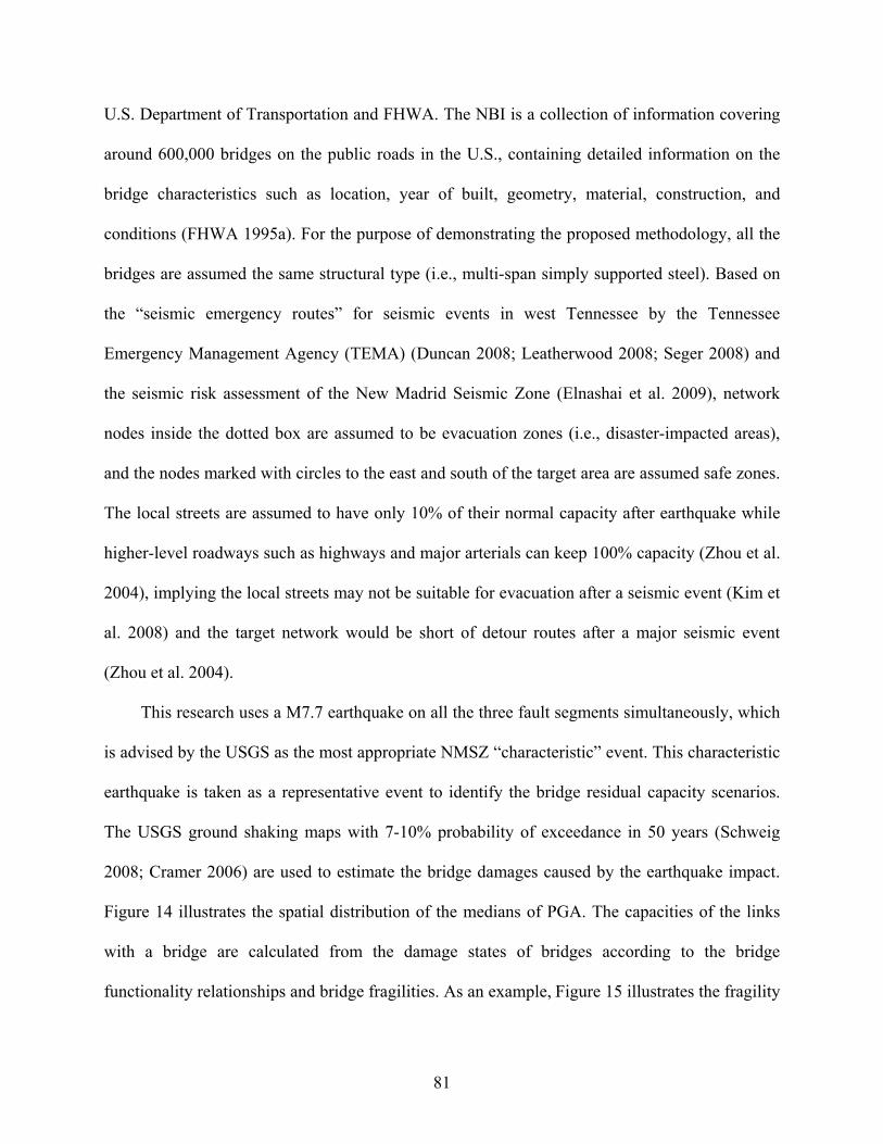
81
U.S. Department of Transportation and FHWA. The NBI is a collection of information covering
around 600,000 bridges on the public roads in the U.S., containing detailed information on the
bridge characteristics such as location, year of built, geometry, material, construction, and
conditions (FHWA 1995a). For the purpose of demonstrating the proposed methodology, all the
bridges are assumed the same structural type (i.e., multi-span simply supported steel). Based on
the “seismic emergency routes” for seismic events in west Tennessee by the Tennessee
Emergency Management Agency (TEMA) (Duncan 2008; Leatherwood 2008; Seger 2008) and
the seismic risk assessment of the New Madrid Seismic Zone (Elnashai et al. 2009), network
nodes inside the dotted box are assumed to be evacuation zones (i.e., disaster-impacted areas),
and the nodes marked with circles to the east and south of the target area are assumed safe zones.
The local streets are assumed to have only 10% of their normal capacity after earthquake while
higher-level roadways such as highways and major arterials can keep 100% capacity (Zhou et al.
2004), implying the local streets may not be suitable for evacuation after a seismic event (Kim et
al. 2008) and the target network would be short of detour routes after a major seismic event
(Zhou et al. 2004).
This research uses a M7.7 earthquake on all the three fault segments simultaneously, which
is advised by the USGS as the most appropriate NMSZ “characteristic” event. This characteristic
earthquake is taken as a representative event to identify the bridge residual capacity scenarios.
The USGS ground shaking maps with 7-10% probability of exceedance in 50 years (Schweig
2008; Cramer 2006) are used to estimate the bridge damages caused by the earthquake impact.
Figure 14 illustrates the spatial distribution of the medians of PGA. The capacities of the links
with a bridge are calculated from the damage states of bridges according to the bridge
functionality relationships and bridge fragilities. As an example, Figure 15 illustrates the fragility
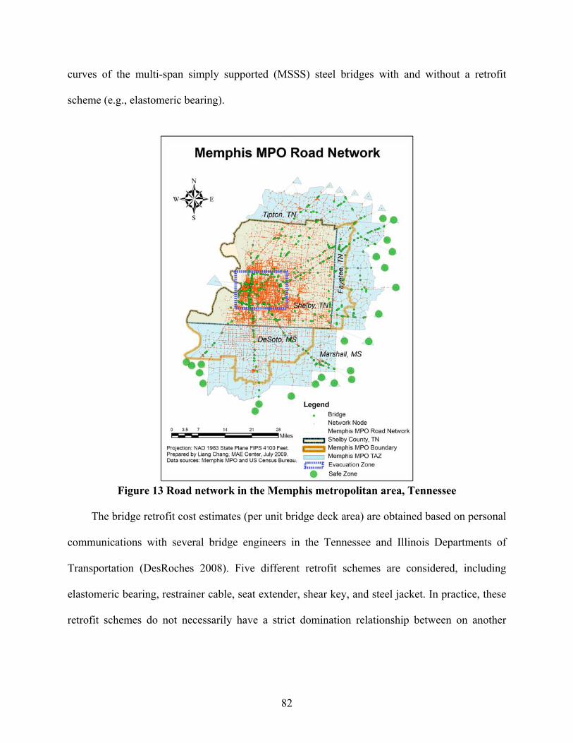
82
curves of the multi-span simply supported (MSSS) steel bridges with and without a retrofit
scheme (e.g., elastomeric bearing).
Figure 13 Road network in the Memphis metropolitan area, Tennessee
The bridge retrofit cost estimates (per unit bridge deck area) are obtained based on personal
communications with several bridge engineers in the Tennessee and Illinois Departments of
Transportation (DesRoches 2008). Five different retrofit schemes are considered, including
elastomeric bearing, restrainer cable, seat extender, shear key, and steel jacket. In practice, these
retrofit schemes do not necessarily have a strict domination relationship between on another
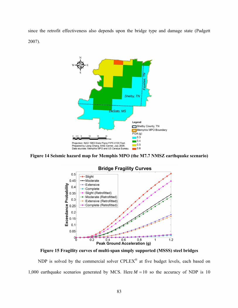
83
since the retrofit effectiveness also depends upon the bridge type and damage state (Padgett
2007).
Figure 14 Seismic hazard map for Memphis MPO (the M7.7 NMSZ earthquake scenario)
Figure 15 Fragility curves of multi-span simply supported (MSSS) steel bridges
NDP is solved by the commercial solver CPLEX® at five budget levels, each based on
1,000 earthquake scenarios generated by MCS. Here 10M so the accuracy of NDP is 10

84
vehicles per hour. The maximum allowable optimality gap for NDP is set to be 0.000001%. The
total solution time for all five budget levels is about 3000 seconds on a personal computer with 2
GHz CPU and about 60 MB of memory usage. The retrofit project effectiveness is a weighted
summation of the expected evacuation flow (now denoted by kFije ) and the expected reduction in
repair cost (denoted by kRije )†; i.e., k k k
ij Fij Rije we e . The weight is set as 100w , such that the
total effectiveness of evacuation flow is about the same as that of the reduced repair costs for
those bridges selected at least once in 1000 scenarios. In practice, other types of effectiveness
measures (e.g., long-term transportation operation efficiency) can also be considered.
The top 20 bridges with the highest effectiveness/cost ratio in the retrofit program list are
shown in Table 6. These bridges have higher effectiveness/cost ratio because they are at the most
vital location of the network and/or are more vulnerable to earthquakes. A simple yet efficient
greedy heuristic is used to select the retrofit projects. Retrofit projects are checked one by one
from the highest effectiveness/cost ratio to the lowest before the budget is exhausted. If two
retrofit schemes are selected for the same bridge during the process, the one with higher
effectiveness will be used. Other cost-effectiveness analysis methods can be found in Patidar et
al. (2007).
Table 6 Top 20 bridges with highest effectiveness-cost ratios
Budget (in millions) / Bridge ID‡ Rank
$0.2 $0.4 $0.6 $0.8 $1.0 I 237 237 237 237 237 II 157 157 157 157 157 III 110 110 110 110 110 IV 139 139 139 139 139 V 138 138 138 138 138
† See Appendix A for the detailed definition of k
Rije . ‡ Bridges with varying cost/effectiveness ratio at various budget levels are in bold font.
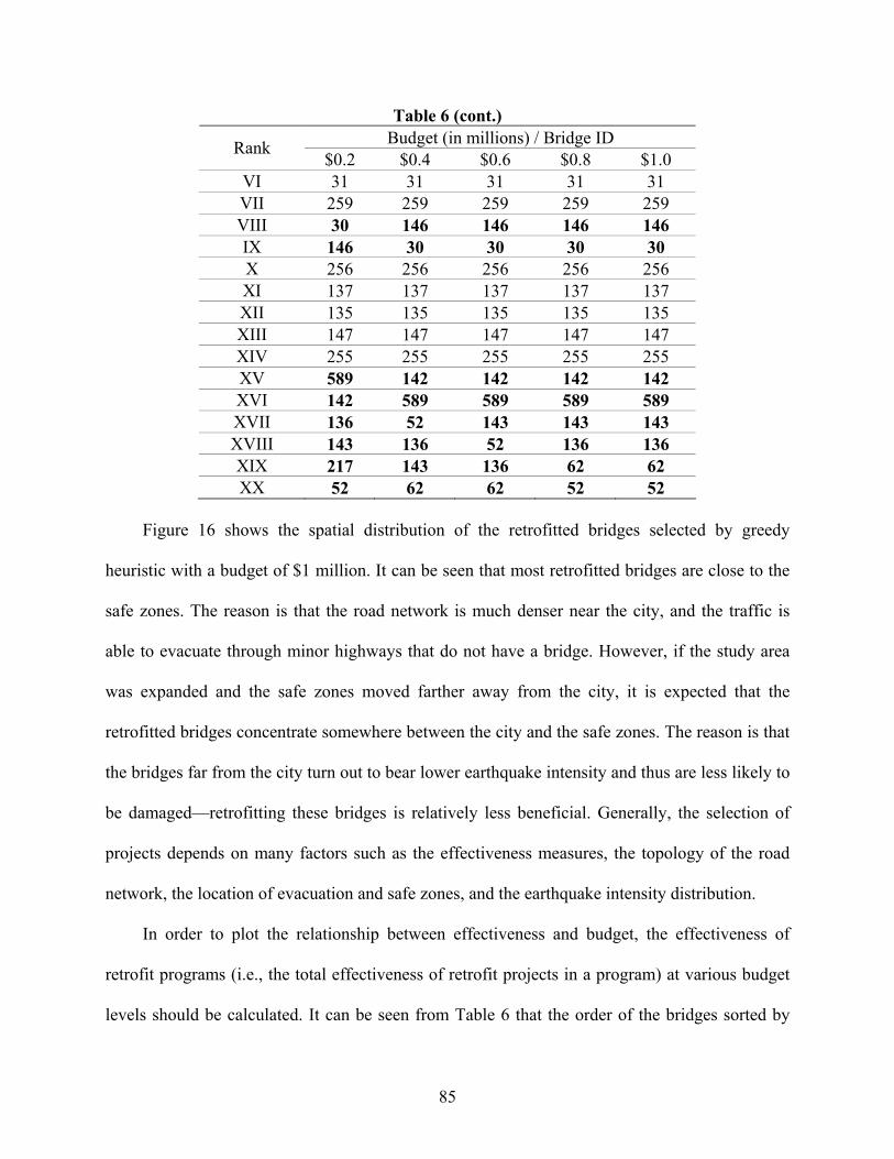
85
Table 6 (cont.) Budget (in millions) / Bridge ID
Rank $0.2 $0.4 $0.6 $0.8 $1.0
VI 31 31 31 31 31 VII 259 259 259 259 259 VIII 30 146 146 146 146 IX 146 30 30 30 30 X 256 256 256 256 256 XI 137 137 137 137 137 XII 135 135 135 135 135 XIII 147 147 147 147 147 XIV 255 255 255 255 255 XV 589 142 142 142 142 XVI 142 589 589 589 589 XVII 136 52 143 143 143 XVIII 143 136 52 136 136 XIX 217 143 136 62 62 XX 52 62 62 52 52
Figure 16 shows the spatial distribution of the retrofitted bridges selected by greedy
heuristic with a budget of $1 million. It can be seen that most retrofitted bridges are close to the
safe zones. The reason is that the road network is much denser near the city, and the traffic is
able to evacuate through minor highways that do not have a bridge. However, if the study area
was expanded and the safe zones moved farther away from the city, it is expected that the
retrofitted bridges concentrate somewhere between the city and the safe zones. The reason is that
the bridges far from the city turn out to bear lower earthquake intensity and thus are less likely to
be damaged—retrofitting these bridges is relatively less beneficial. Generally, the selection of
projects depends on many factors such as the effectiveness measures, the topology of the road
network, the location of evacuation and safe zones, and the earthquake intensity distribution.
In order to plot the relationship between effectiveness and budget, the effectiveness of
retrofit programs (i.e., the total effectiveness of retrofit projects in a program) at various budget
levels should be calculated. It can be seen from Table 6 that the order of the bridges sorted by

86
effectiveness/cost ratio only changes slightly across different budgets (the bridges with different
ranks at various budget levels are highlighted by bold font). Therefore, the effectiveness
calculated from the $1 million budget case can be used to create retrofit programs in other
budgets (including the zero budget case) without losing much accuracy. For each budget, greedy
heuristic is used to select the retrofit projects. The greedy algorithm terminates as soon as the
cost of the currently checked project exceeds the remaining budget, and then the budget is
recalculated as the sum of the costs of all selected retrofit projects. In this way, it can be ensured
that there is no remaining budget and the created retrofit program is optimum.
Figure 16 Spatial distribution of bridge retrofit program under $1 million budget
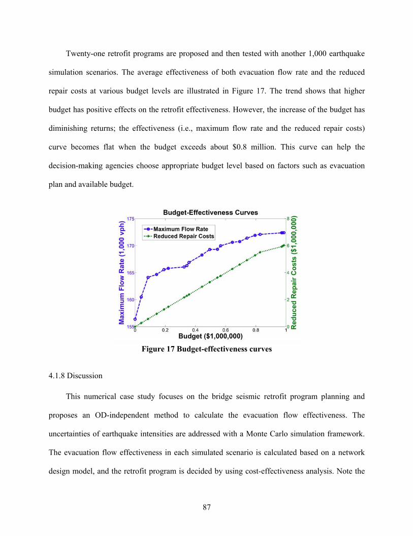
87
Twenty-one retrofit programs are proposed and then tested with another 1,000 earthquake
simulation scenarios. The average effectiveness of both evacuation flow rate and the reduced
repair costs at various budget levels are illustrated in Figure 17. The trend shows that higher
budget has positive effects on the retrofit effectiveness. However, the increase of the budget has
diminishing returns; the effectiveness (i.e., maximum flow rate and the reduced repair costs)
curve becomes flat when the budget exceeds about $0.8 million. This curve can help the
decision-making agencies choose appropriate budget level based on factors such as evacuation
plan and available budget.
Figure 17 Budget-effectiveness curves
4.1.8 Discussion
This numerical case study focuses on the bridge seismic retrofit program planning and
proposes an OD-independent method to calculate the evacuation flow effectiveness. The
uncertainties of earthquake intensities are addressed with a Monte Carlo simulation framework.
The evacuation flow effectiveness in each simulated scenario is calculated based on a network
design model, and the retrofit program is decided by using cost-effectiveness analysis. Note the
88
scope of evacuation is limited to the short-term period and steady-state flows and the evacuation
zones are assumed to have sufficient demands during the evacuation process.
The proposed methodology is demonstrated with a real-world case study in the Memphis
metropolitan area. Results from the numerical example show that the effectiveness of retrofit
programs increases with the budget with diminishing returns. Specifically, the maximum flow
rate is positively correlated with the reduced repair costs, which increases linearly with the
available budget. The results from the case study also suggest the presence of optimum amount
of allocated resources (i.e., critical level of budget), beyond which additional retrofitting
becomes less effective. The budget-effectiveness curve is consistent with the intuition that higher
budget levels lead to more retrofit effectiveness but with diminishing effectiveness.
The demonstrated network-flow capacity-based NBSR methodology can be used to (i)
evaluate post-earthquake performance of transportation systems, (ii) identify retrofit project
priorities, (iii) plan budget from a systematic viewpoint, and (iv) improve the disaster resilience
of transportation systems under economic constraints. The proposed methodology also allows
more general effectiveness measurements to help government agencies and emergency managers
make better decisions.
4.2 Reliability of Network Reachability
This section discusses the reliability of network reachability of transportation infrastructure
systems by employing the recursive decomposition algorithm. In an emergency, it is critical to
identify the passable ingress and egress routes for emergency response within a short time frame,
e.g., to send search and rescue teams into the impacted area immediately after a disruptive
earthquake. To emergency managers and rescue workers, of great concern are the knowledge of
potential bridge collapse or road closure due to seismic impact, and whether the structural
89
damage interrupts the integrity or connectivity of transportation systems. The reliability of
network reachability is an appropriate metric under such conditions.
4.2.1 Recursive Decomposition Algorithm for Reachability Reliability
Figure 18 illustrates the key RDA procedures to evaluate the system reliability by
decomposing a simple benchmark network. To evaluate the network connectivity between the
source node s and terminal node t (e.g., the impact zone and safe zone), first an arbitrary
shortest path { 1 2 }s t between the source and terminal is identified. Based on the
identified path, the network is then decomposed recursively into sub-graphs until there is no path
existed between the source-terminal node-pair in all sub-graphs. For the benchmark network
shown in Figure 18, the RDA identifies five disjoint link sets { 1 1 2L , 2 1 4 5L ,
3 1 2 4 5L , 4 1 4 5 3 2L , 5 1 2 4 3 5L } and six disjoint cut sets { 1 1 4F ,
2 1 2 4 5F , 3 1 4 5 3F , 4 1 4 5 3 2F , 5 1 2 4 3F , 6 1 2 4 3 5F }, in which
the numbers with and without an upper bar indicate the failures and survivals of the
corresponding network components (e.g., edges), respectively.
Before applying the RDA to the numerical case study, its correctness of implementation is
verified by comparing the system accessibilities between the source node and sink node for
twenty commonly-used benchmark networks. The verification of the RDA is detailed in
Appendix B.

90
3 1 2 4 5L
4 1 4 5 3 2L 5 1 2 4 3 5L 1 1 4F 2 1 2 4 5F
3 1 4 5 3F 4 1 4 5 3 2F 5 1 2 4 3F 6 1 2 4 3 5F
1 1 2L
2 1 4 5L
Figure 18 Illustration of the recursive decomposition algorithm
4.2.2 Numerical Example: the Sioux-Falls Road Network
The RDA is illustrated by using the Sioux-Falls network (shown in Figure 19) as a
numerical example. The bridge information is described in Table 3. The impacted zones (i.e.,
evacuation zones) are considered the source nodes and a virtual sink node is added to the graph
to facilitate finding the node-pair connectivity for the multi-source and multi-terminal network
model. The failure probabilities of bridges are calculated by using the bridge fragility curves and
the hazard maps given in Section 4.1.5.
Figure 20 shows the probability that the impacted zone (i.e., Node 1) will be disconnected
from safe zones. Note that the consideration of spatial correlation of ground motion affects the
estimates of system reliability but not significantly. An additional investigation on the correlation
of structural damage would be necessary to obtain more reliable results, but is beyond the scope
of this study. Figure 21 gives the disconnection probabilities of several selected network nodes,
in which the intra-event uncertainty 2 is 0.1 and the correlation length b is 4 km.
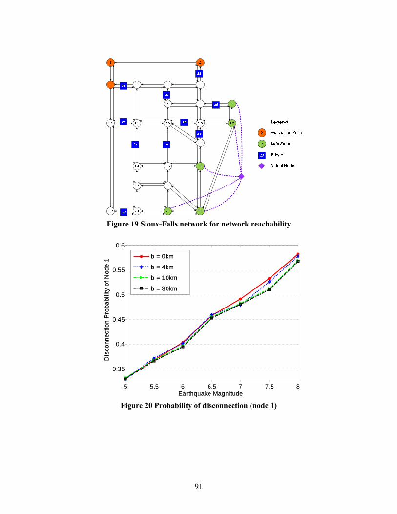
91
Figure 19 Sioux-Falls network for network reachability
5 5.5 6 6.5 7 7.5 8
0.35
0.4
0.45
0.5
0.55
0.6
Earthquake Magnitude
Dis
conn
ect
ion
Pro
ba
bilit
y o
f N
ode
1
b = 0km
b = 4km
b = 10km
b = 30km
Figure 20 Probability of disconnection (node 1)
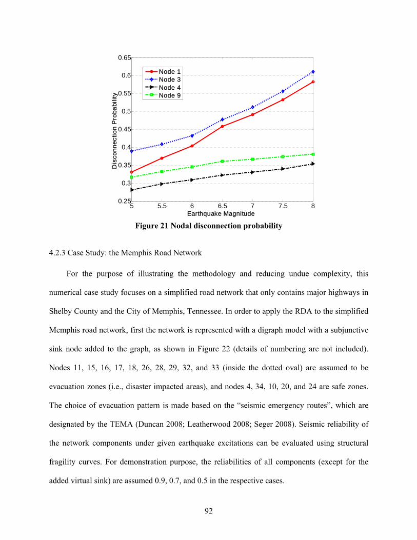
92
5 5.5 6 6.5 7 7.5 80.25
0.3
0.35
0.4
0.45
0.5
0.55
0.6
0.65
Earthquake Magnitude
Dis
con
ne
ctio
n P
roba
bilit
y
Node 1Node 3Node 4Node 9
Figure 21 Nodal disconnection probability
4.2.3 Case Study: the Memphis Road Network
For the purpose of illustrating the methodology and reducing undue complexity, this
numerical case study focuses on a simplified road network that only contains major highways in
Shelby County and the City of Memphis, Tennessee. In order to apply the RDA to the simplified
Memphis road network, first the network is represented with a digraph model with a subjunctive
sink node added to the graph, as shown in Figure 22 (details of numbering are not included).
Nodes 11, 15, 16, 17, 18, 26, 28, 29, 32, and 33 (inside the dotted oval) are assumed to be
evacuation zones (i.e., disaster impacted areas), and nodes 4, 34, 10, 20, and 24 are safe zones.
The choice of evacuation pattern is made based on the “seismic emergency routes”, which are
designated by the TEMA (Duncan 2008; Leatherwood 2008; Seger 2008). Seismic reliability of
the network components under given earthquake excitations can be evaluated using structural
fragility curves. For demonstration purpose, the reliabilities of all components (except for the
added virtual sink) are assumed 0.9, 0.7, and 0.5 in the respective cases.
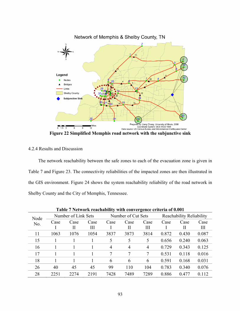
93
Figure 22 Simplified Memphis road network with the subjunctive sink
4.2.4 Results and Discussion
The network reachability between the safe zones to each of the evacuation zone is given in
Table 7 and Figure 23. The connectivity reliabilities of the impacted zones are then illustrated in
the GIS environment. Figure 24 shows the system reachability reliability of the road network in
Shelby County and the City of Memphis, Tennessee.
Table 7 Network reachability with convergence criteria of 0.001
Number of Link Sets Number of Cut Sets Reachability Reliability Node No. Case
I Case
II Case III
Case I
Case II
Case III
Case I
Case II
Case III
11 1063 1076 1054 3837 3873 3814 0.872 0.430 0.087
15 1 1 1 5 5 5 0.656 0.240 0.063
16 1 1 1 4 4 4 0.729 0.343 0.125
17 1 1 1 7 7 7 0.531 0.118 0.016
18 1 1 1 6 6 6 0.591 0.168 0.031
26 40 45 45 99 110 104 0.783 0.340 0.076
28 2251 2274 2191 7428 7489 7289 0.886 0.477 0.112
Subjunctive Sink
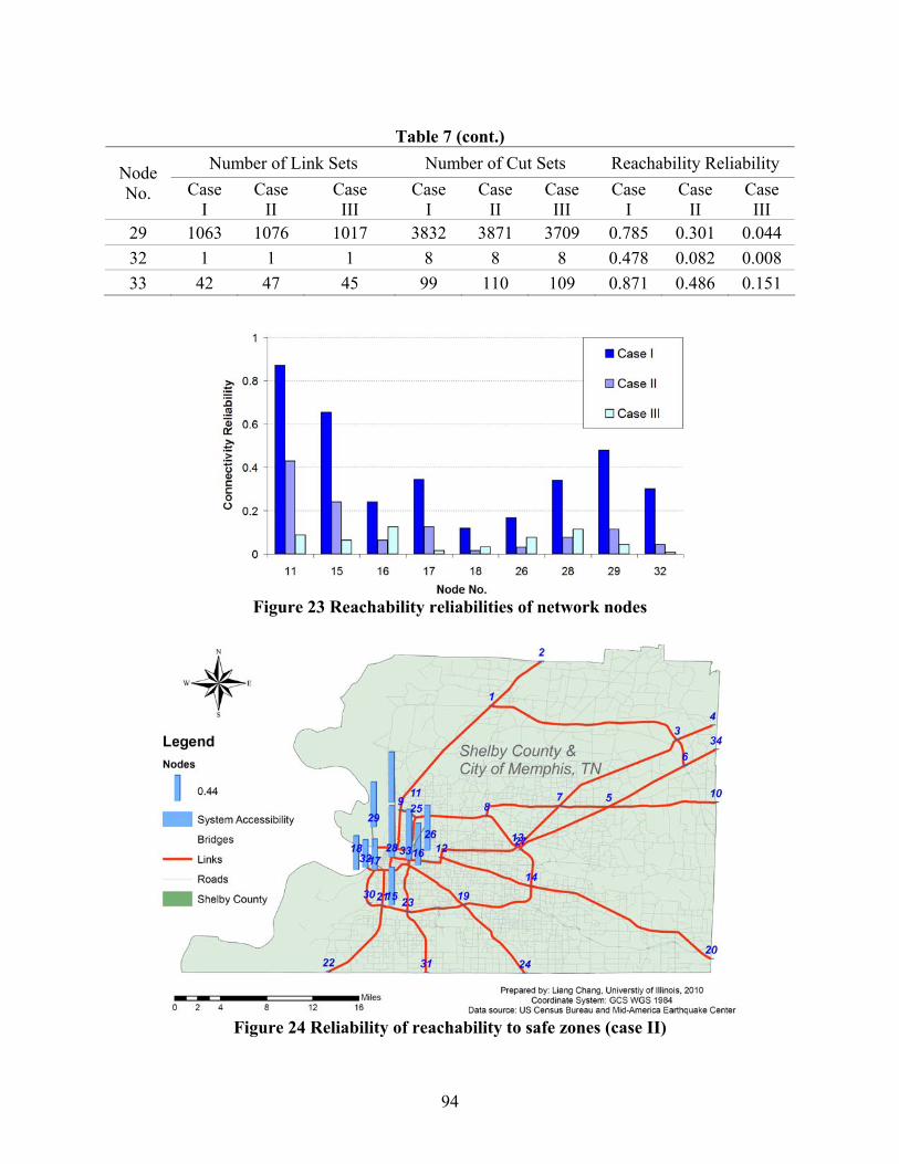
94
Table 7 (cont.)
Number of Link Sets Number of Cut Sets Reachability Reliability Node No. Case
I Case
II Case III
Case I
Case II
Case III
Case I
Case II
Case III
29 1063 1076 1017 3832 3871 3709 0.785 0.301 0.044
32 1 1 1 8 8 8 0.478 0.082 0.008
33 42 47 45 99 110 109 0.871 0.486 0.151
Figure 23 Reachability reliabilities of network nodes
Figure 24 Reliability of reachability to safe zones (case II)
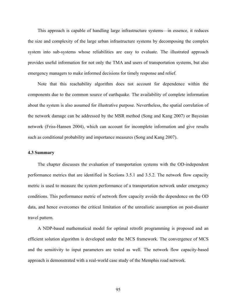
95
This approach is capable of handling large infrastructure systems—in essence, it reduces
the size and complexity of the large urban infrastructure systems by decomposing the complex
system into sub-systems whose reliabilities are easy to evaluate. The illustrated approach
provides useful information for not only the TMA and users of transportation systems, but also
emergency managers to make informed decisions for timely response and relief.
Note that this reachability algorithm does not account for dependence within the
components due to the common source of earthquake. The availability of complete information
about the system is also assumed for illustrative purpose. Nevertheless, the spatial correlation of
the network damage can be addressed by the MSR method (Song and Kang 2007) or Bayesian
network (Friss-Hansen 2004), which can account for incomplete information and give results
such as conditional probability and importance measures (Song and Kang 2007).
4.3 Summary
The chapter discusses the evaluation of transportation systems with the OD-independent
performance metrics that are identified in Sections 3.5.1 and 3.5.2. The network flow capacity
metric is used to measure the system performance of a transportation network under emergency
conditions. This performance metric of network flow capacity avoids the dependence on the OD
data, and hence overcomes the critical limitation of the unrealistic assumption on post-disaster
travel pattern.
A NDP-based mathematical model for optimal retrofit programming is proposed and an
efficient solution algorithm is developed under the MCS framework. The convergence of MCS
and the sensitivity to input parameters are tested as well. The network flow capacity-based
approach is demonstrated with a real-world case study of the Memphis road network.

96
In addition, the network reachability, or the connectivity reliability between the safe zones
and evacuation zones is discussed and a sensitivity analysis is performed for relevant factors.
The network reachability of the Memphis road network is quantified by employing the state-of-
the-art RDA. Based on such results, the regions that are potentially difficult to reach after a
disruptive earthquake can be identified to make informed emergency response plans.
The proposed OD-independent performance metrics extend the existing NBSR framework
and provide essential information for emergency response, efficient retrofit prioritization, and
budget planning procedures. The following chapter, Chapter 5 discusses post-earthquake travel
demand modeling and evaluates the performance of transportation networks with the travel delay
cost metrics.
97
CHAPTER V MODELING THE POST-EARTHQUAKE TRAVEL DEMAND
5.1 Introduction
The state-of-the-art seismic mitigation measures for transportation systems have focused on
earthquake design and retrofit of transportation infrastructure. In emergency situations, however,
the operation of highway systems is equally important. The traffic flow under emergency
conditions (e.g., a damaging earthquake) may be significantly different from the traffic under
“normal” conditions due to the drastic changes in post-event demand and the deteriorated
network capacities as well. Conventional travel demand models such as the FDM are limited and
unsuitable in post-earthquake emergency situations due to unrealistic assumptions (Shinozuka et
al. 2005; Fan 2006; Werner et al. 2006; Kiremidjian et al. 2007).
Employing travel delay cost metrics for the performance evaluation of transportation
systems, this chapter focuses on the development of demand simulation models that account for
the change of traffic pattern after a damaging earthquake. Because travel delay cost metrics are
highly dependent upon the detailed OD travel demand information, a methodology to model the
post-earthquake travel demand is first given in Section 5.2. This model approximates the
“abnormal” travel demand by adopting several general principles. The post-earthquake travel
patterns are characterized by considering the effects of structural damage and emergency
facilities on travel behavior. Section 5.3 presents the results from the numerical case studies, in
which the performance is measured by the travel delay cost metrics. Section 5.4 discusses the
results and summarizes the major conclusions.
98
5.2 Methodology for Travel Demand Modeling
Based on the review of travel demand models and post-earthquake travel patterns in Section
2.2.1.3, this section presents a methodology to model post-earthquake travel demand and
evaluate the system performance with travel delay cost metrics. Note the proposed methodology
does not attempt to provide “real-time” post-earthquake traffic simulation. Instead, it aims at
providing general principles and procedures for emergency training and planning purposes. The
major assumptions and key procedures of the proposed methodology are presented in the
following subsections.
5.2.1 Scenarios and Major Assumptions
Earthquake occurrence time significantly affects the number of casualties and their spatial
distribution since traffic patterns and population distribution in different periods are distinct. For
this reason, useful earthquake scenarios for demand modeling should specifically consider the
occurrence time of day (e.g., morning and late-night period), days of the week, and the seasons
of the year, etc.
In this study, two hypothetical scenarios are developed to postulate and model the impact of
a no-notice event on transportation systems—one occurring during morning rush hours
(hereinafter referred to as the day scenario), and another at late night (hereinafter referred to as
the night scenario). Both scenarios are assumed to occur without the presence of adverse weather
conditions such as rain or snow. The hypothetical scenario earthquakes will leave several bridges
(e.g., major river crossings) and essential facilities (e.g., schools) severely damaged. Traffic
management measures may include closures of highways due to damages of ramps or pavements,
demolished or severely undermined bridges, or evacuation of regions with HAZMAT release, etc.
These scenarios can provide emergency response teams with optimal transportation pathways for
99
rapid emergency ingress and egress, and help evaluate emergency routes performance and
estimate congestion under extreme events.
Modeling travel behavior and route choices, even under normal conditions, is challenging.
Approximation of travel demand following earthquakes is challenging due to many socio-
economic uncertainty aspects involved (Fan 2006). To simplify the complex problem of travel
demand modeling, several general assumptions are made on post-earthquake travel behavior and
emergency traffic management measures (Chang et al. 2009):
This study assumes that people will evacuate directly from their current locations
immediately after earthquakes. This assumption is made because under pre-noticed
scenarios such as hurricane evacuation (e.g., 24 or 48 hours before the landfall), it is
reasonable to assume that people will be either at home, or returning home before
beginning the evacuating. While under the no-notice earthquake scenarios, there is
no time or considerably less time to return home or go to other places to pick up
their relatives or friends (Noh et al. 2009). Social vulnerability to disasters such as
race, gender, and social inequality has a crucial role in shaping the evacuation
patterns, but is beyond the scope of this study.
Trip generation is assumed proportional to the size of affected population, and trip
generation rates common within the TAZ. Such homogenous assumption on the
TAZ is based on the cross-classification methods, which aggregate the population
into certain homogenous groups based on their geographic locations and socio-
economic characteristics such as auto ownership and income, etc. (EWGCC 2003;
Chatterjee and Venigalla 2004). Moreover, because the pattern of population
distribution changes at different periods of time, the number of population during

100
day time and at night, if available, will be taken from the 2000 U.S. census for the
trip generation of the morning scenario and late night scenario, respectively.
Depending on the presence of attractants (e.g., hospitals or emergency shelter) and
repellents (e.g., HAZMAT release, fire following earthquake, or damaged facilities),
the TAZ can be classified into four zone types (Figure 25). The underlying
assumptions are that: (i) if a zone does not have damaged facilities, its trip
production will not be affected by the earthquake, while the trip production will
increase in the affected zones due to facilities damage, fire or hazmat release, and (ii)
if a zone does not offer emergency shelters or hospitals, its trip attraction will
remain unchanged; while the trip attraction will increase because of the presence of
emergency shelters and/or hospitals. Figure 26 illustrates the assumptions on zone
types and Table 8 summarizes the characteristics of trip generation for each of the
zone type.
Bridges with at least major damage are assumed to be impassable and closed
(Yashinsky 1998). Buildings with at least moderate damage will be evacuated§.
Special group population in schools and colleges, hospitals, and jails may be
required to evacuate due to structural damage (Schultz et al. 2003).
Neighboring region of HAZMAT release due to the damage to HAZMAT plants or
explosion of nuclear power plants requires a full evacuation. Emergency shelters
and hospitals are assumed attractive sites to injured or displaced people. The
attracted trips to shelters and hospitals are proportional to their capacities (e.g., the
number of beds in a hospital).
§ Due to the lack of specific population/square footage information for individual buildings , two additional assumptions are made: (i) damage is evenly distributed across occupancy types, and (ii) population or square footage is evenly distributed within the same occupancy category.
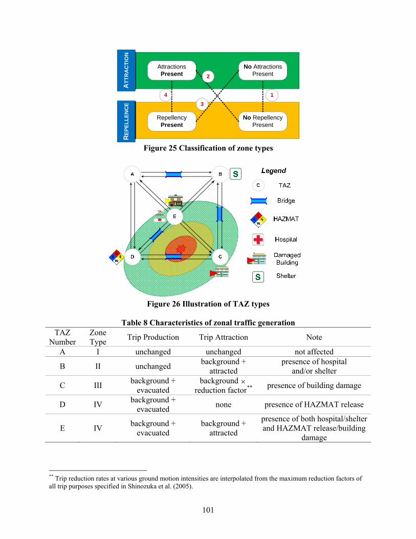
101
No Repellency Present
AttractionsPresent
No AttractionsPresent
RepellencyPresent
RE
PE
LL
EN
CE
AT
TR
AC
TIO
N
2
1
3
4
Figure 25 Classification of zone types
Figure 26 Illustration of TAZ types
Table 8 Characteristics of zonal traffic generation
TAZ Number
Zone Type
Trip Production Trip Attraction Note
A I unchanged unchanged not affected
B II unchanged background +
attracted presence of hospital
and/or shelter
C III background +
evacuated background
reduction factor** presence of building damage
D IV background +
evacuated none presence of HAZMAT release
E IV background +
evacuated background +
attracted
presence of both hospital/shelter and HAZMAT release/building
damage
** Trip reduction rates at various ground motion intensities are interpolated from the maximum reduction factors of all trip purposes specified in Shinozuka et al. (2005).
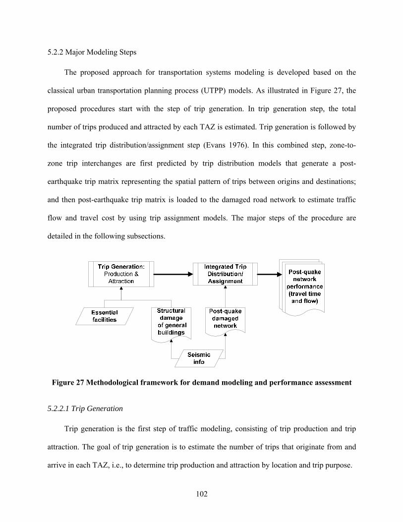
102
5.2.2 Major Modeling Steps
The proposed approach for transportation systems modeling is developed based on the
classical urban transportation planning process (UTPP) models. As illustrated in Figure 27, the
proposed procedures start with the step of trip generation. In trip generation step, the total
number of trips produced and attracted by each TAZ is estimated. Trip generation is followed by
the integrated trip distribution/assignment step (Evans 1976). In this combined step, zone-to-
zone trip interchanges are first predicted by trip distribution models that generate a post-
earthquake trip matrix representing the spatial pattern of trips between origins and destinations;
and then post-earthquake trip matrix is loaded to the damaged road network to estimate traffic
flow and travel cost by using trip assignment models. The major steps of the procedure are
detailed in the following subsections.
Figure 27 Methodological framework for demand modeling and performance assessment
5.2.2.1 Trip Generation
Trip generation is the first step of traffic modeling, consisting of trip production and trip
attraction. The goal of trip generation is to estimate the number of trips that originate from and
arrive in each TAZ, i.e., to determine trip production and attraction by location and trip purpose.
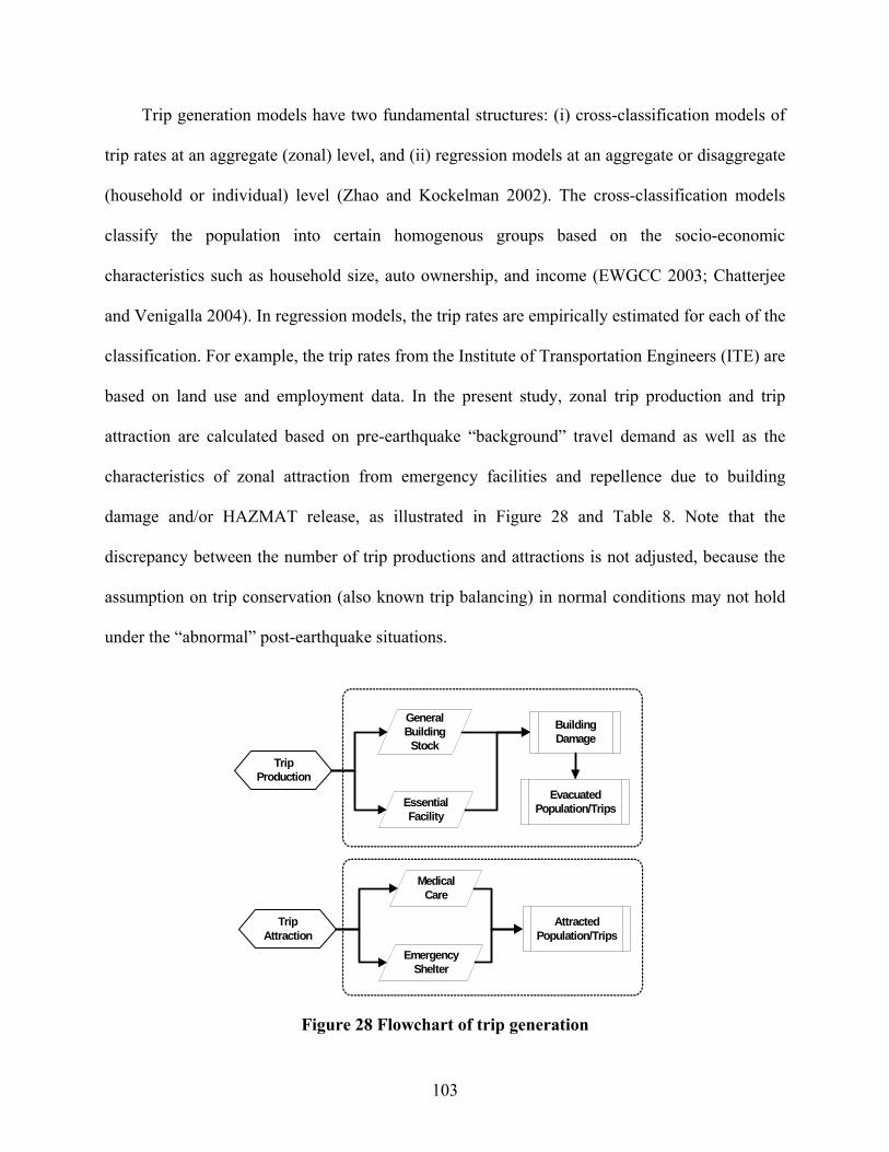
103
Trip generation models have two fundamental structures: (i) cross-classification models of
trip rates at an aggregate (zonal) level, and (ii) regression models at an aggregate or disaggregate
(household or individual) level (Zhao and Kockelman 2002). The cross-classification models
classify the population into certain homogenous groups based on the socio-economic
characteristics such as household size, auto ownership, and income (EWGCC 2003; Chatterjee
and Venigalla 2004). In regression models, the trip rates are empirically estimated for each of the
classification. For example, the trip rates from the Institute of Transportation Engineers (ITE) are
based on land use and employment data. In the present study, zonal trip production and trip
attraction are calculated based on pre-earthquake “background” travel demand as well as the
characteristics of zonal attraction from emergency facilities and repellence due to building
damage and/or HAZMAT release, as illustrated in Figure 28 and Table 8. Note that the
discrepancy between the number of trip productions and attractions is not adjusted, because the
assumption on trip conservation (also known trip balancing) in normal conditions may not hold
under the “abnormal” post-earthquake situations.
Building Damage
General Building Stock
Evacuated Population/Trips
Trip Production
Essential Facility
Trip Attraction
Medical Care
Emergency Shelter
Attracted Population/Trips
Figure 28 Flowchart of trip generation

104
In this study, the generated trips related to residential buildings are assumed proportional to
the affected population in a TAZ. While trips related to commercial or industrial buildings are
assumed proportional to the affected square footage and are estimated using the ITE trip rates.
To estimate the travel demand stemming from structural damage, detailed information is
required on the composition of building inventory, the damage distribution amongst the
inventory, and the population associated with the damaged buildings. The attracted trips to
emergency shelters and hospitals are estimated based on their respective capacities, e.g., the
number of beds in a hospital and the post-impact capacity of an emergency shelter.
Travel demand (in the unit of vehicle trips) is aggregated at the TAZ level. Population data
is aggregated at census tract level, while the building damage information may be available only
at aggregated level, or at individual structure level for a limited areas††.
If the damage information is unavailable for individual buildings (i.e., the aggregated
damage case), the number of damaged buildings in each occupancy category can be estimated
based on the total number of damaged buildings in the census tract and the damage probability of
the structural fragility curves (Figure 29). Since the composition of building occupancy types is
unknown, it is assumed that the number of damaged buildings of certain occupancy type is
proportional to the exceeding probability of structural limit states specified in the representative
fragility curves. In other words, the more vulnerable (higher exceeding probability) the building
is to earthquake, the higher percentage (or more probable) of damaged buildings is in the
inventory. For example, given the ground motion intensity x , the exceeding probabilities are 0.4
and 0.85 (Figure 29) for concrete and wood structure, respectively. This means the number of
damaged residential buildings would be approximately 2.1 times of that of damaged commercial
†† Individual building damage information can be obtained only for the City of Memphis and Shelby County, Tennessee with the building inventory provided in MAEViz.
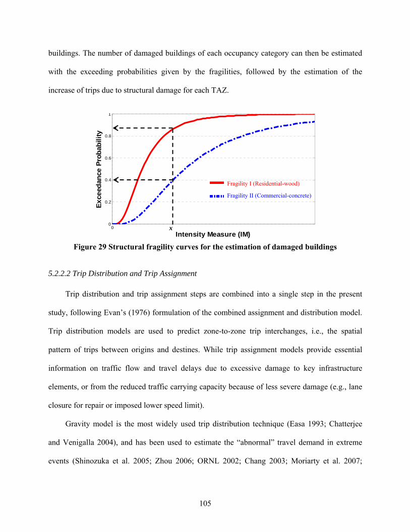
105
buildings. The number of damaged buildings of each occupancy category can then be estimated
with the exceeding probabilities given by the fragilities, followed by the estimation of the
increase of trips due to structural damage for each TAZ.
00
0.2
0.4
0.6
0.8
1
Intensity Measure (IM)
Ex
ceed
ance
Pro
bab
ilit
y
Figure 29 Structural fragility curves for the estimation of damaged buildings
5.2.2.2 Trip Distribution and Trip Assignment
Trip distribution and trip assignment steps are combined into a single step in the present
study, following Evan’s (1976) formulation of the combined assignment and distribution model.
Trip distribution models are used to predict zone-to-zone trip interchanges, i.e., the spatial
pattern of trips between origins and destines. While trip assignment models provide essential
information on traffic flow and travel delays due to excessive damage to key infrastructure
elements, or from the reduced traffic carrying capacity because of less severe damage (e.g., lane
closure for repair or imposed lower speed limit).
Gravity model is the most widely used trip distribution technique (Easa 1993; Chatterjee
and Venigalla 2004), and has been used to estimate the “abnormal” travel demand in extreme
events (Shinozuka et al. 2005; Zhou 2006; ORNL 2002; Chang 2003; Moriarty et al. 2007;
Fragility I (Residential-wood)
Fragility II (Commercial-concrete)
x

106
Wakabayashi and Kameda 1992). Other popular trip distribution models include the growth
factor models such as the Fratar Model and the Detroit Model. These growth factor models are
an extrapolation of the previously surveyed OD data by assuming that future transportation
distribution has similar pattern as the current one, and hence restricted to long-range forecasting
travel demand in an urban area. Since it is difficult to obtain post-earthquake OD data, gravity
model is employed to determine where trips go (trip distribution) in the present study.
The gravity model is in analogy with Newton’s law of gravity—the trip interchange
between origin and destination zones is proportional to activities represented by trip generation,
and inversely proportional to the separation (impedance) between the zones, which is usually
represented as a function of travel time. The gravity model, subject to the constraints of trip
production and trip attraction, is defined as follows:
( )i j
ij i jij
O DT A B
F t (40)
where ijT is the number of trips from zone i to zone j , iA is the constant to balance trips
originating from zone i , jB is the constant to balance trips destined for zone j , iO is the
number of trip production in zone i , jD the number of trip attraction in zone j , ijt the
impedance (travel time or cost) from zone i to zone j , and ( )ijF t the deterrence function,
which is usually inversely related the zone separation in a form of Gamma, power, or
exponential functions. This doubly constrained gravity distribution model ensures that the
resultant trip matrix matches the productions and attractions of each TAZ. The output trip matrix
(i.e., the post-earthquake travel demand) is then loaded to the transportation networks with traffic
assignment models to simulate the traffic flow over the roads following the earthquake.

107
Trip assignment, also known as traffic assignment, provides essential information of traffic
flow and travel costs. The travel delay cost metrics (e.g., TSTT) obtained by traffic assignment
models are used to measure the functional loss of transportation system. The Network Loss
Analysis (NLA) module in MAEViz, MAE Center’s comprehensive seismic risk assessment
package, is employed for simulating the post-disaster emergency traffic.
Both static and dynamic traffic assignment models are implemented in the NLA module
under the user equilibrium assumptions. The DUE model is one of the macro-simulators based
on equations stemming from analogies with fluid flows in network, and does not attempt to track
the behavior of individual vehicles. To ensure the correctness of the implementation of DUE
model, the TSTT results are first validated by checking their corresponding upper and lower
bounds (see Appendix D).
The DUE model is static and only copes with steady state conditions, which may not be
adequate in the dynamic, and sometimes chaotic environment of an emergency evacuation (Pidd
et al. 1996). In order to model the time-dependent traffic over the network, the NLA module
incorporates the Visual Interactive System for Transport Algorithms (VISTA), which is the state-
of-the-art DTA model built upon the enhanced CTM and supports for variable-sized cells and
signalized intersections (Ziliaskopoulos and Waller 2000).
5.3 Case Studies
5.3.1 Sioux-Falls Road Network
The proposed methodology is illustrated by the Sioux-Falls network (Figure 30) as a
numerical case study. Nodes 1, 2, and 3 are assumed to be the evacuation zones (i.e., impacted
area with building damage or HAZMAT release), and nodes 7, 18, 19, 20, and 21 to be the safe
zones with emergency shelters and/or medical facilities.
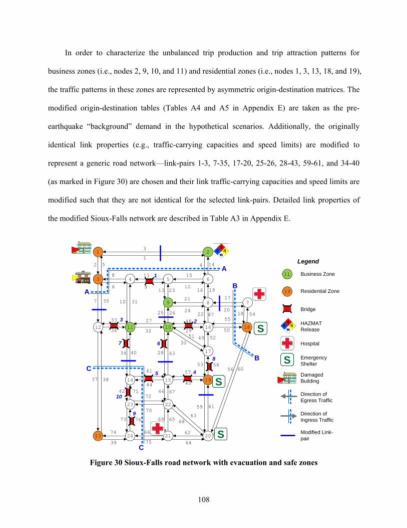
108
In order to characterize the unbalanced trip production and trip attraction patterns for
business zones (i.e., nodes 2, 9, 10, and 11) and residential zones (i.e., nodes 1, 3, 13, 18, and 19),
the traffic patterns in these zones are represented by asymmetric origin-destination matrices. The
modified origin-destination tables (Tables A4 and A5 in Appendix E) are taken as the pre-
earthquake “background” demand in the hypothetical scenarios. Additionally, the originally
identical link properties (e.g., traffic-carrying capacities and speed limits) are modified to
represent a generic road network—link-pairs 1-3, 7-35, 17-20, 25-26, 28-43, 59-61, and 34-40
(as marked in Figure 30) are chosen and their link traffic-carrying capacities and speed limits are
modified such that they are not identical for the selected link-pairs. Detailed link properties of
the modified Sioux-Falls network are described in Table A3 in Appendix E.
54
1
8
4 5 63
2
15 19
17
18
7
12 11 10 16
9
20
23 22
14
13 24 21
3
12
6
8
9
11
5
15
122313
21
16 19
17
2018
55
50
48
2951 49 52
58
24
27
32
33
36
7 35
4034
41
44
57
45
72
70
46 67
69 65
25
28 43
53
59 61
56 60
66 62
6863
7673
30
7142
647539
74
37 38
26
4 14
22 47
10 31
1
23
7 6
8
45
10
9
A
A
C
C
B
B
S
S
S
11
19
Business Zone
Residential Zone
Bridge
S
HAZMATRelease
Hospital
Emergency Shelter
Legend
Damaged Building
Direction of Egress Traffic
Direction of Ingress Traffic
Modified Link-pair
Figure 30 Sioux-Falls road network with evacuation and safe zones
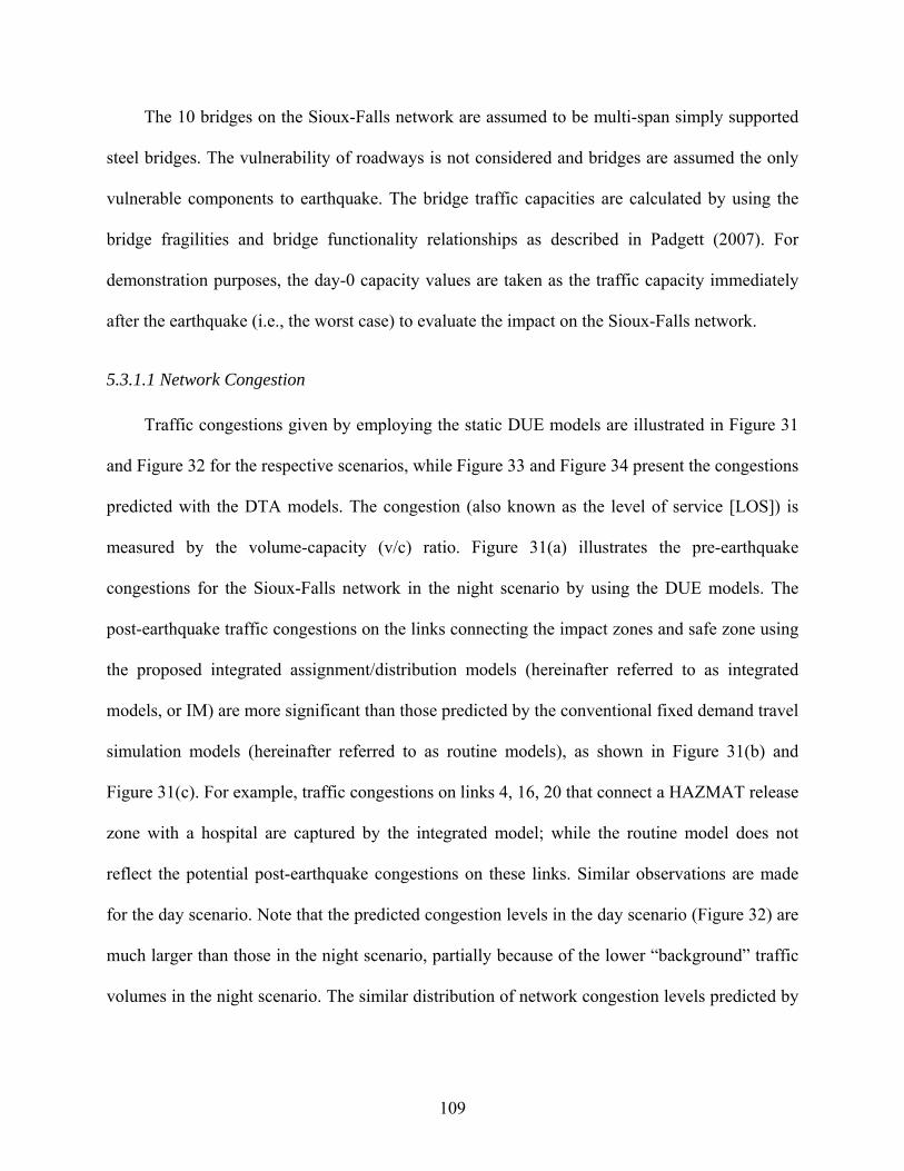
109
The 10 bridges on the Sioux-Falls network are assumed to be multi-span simply supported
steel bridges. The vulnerability of roadways is not considered and bridges are assumed the only
vulnerable components to earthquake. The bridge traffic capacities are calculated by using the
bridge fragilities and bridge functionality relationships as described in Padgett (2007). For
demonstration purposes, the day-0 capacity values are taken as the traffic capacity immediately
after the earthquake (i.e., the worst case) to evaluate the impact on the Sioux-Falls network.
5.3.1.1 Network Congestion
Traffic congestions given by employing the static DUE models are illustrated in Figure 31
and Figure 32 for the respective scenarios, while Figure 33 and Figure 34 present the congestions
predicted with the DTA models. The congestion (also known as the level of service [LOS]) is
measured by the volume-capacity (v/c) ratio. Figure 31(a) illustrates the pre-earthquake
congestions for the Sioux-Falls network in the night scenario by using the DUE models. The
post-earthquake traffic congestions on the links connecting the impact zones and safe zone using
the proposed integrated assignment/distribution models (hereinafter referred to as integrated
models, or IM) are more significant than those predicted by the conventional fixed demand travel
simulation models (hereinafter referred to as routine models), as shown in Figure 31(b) and
Figure 31(c). For example, traffic congestions on links 4, 16, 20 that connect a HAZMAT release
zone with a hospital are captured by the integrated model; while the routine model does not
reflect the potential post-earthquake congestions on these links. Similar observations are made
for the day scenario. Note that the predicted congestion levels in the day scenario (Figure 32) are
much larger than those in the night scenario, partially because of the lower “background” traffic
volumes in the night scenario. The similar distribution of network congestion levels predicted by
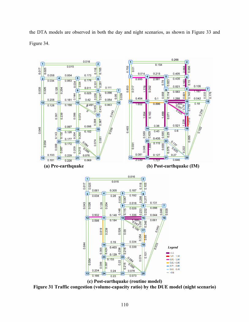
110
the DTA models are observed in both the day and night scenarios, as shown in Figure 33 and
Figure 34.
(a) Pre-earthquake (b) Post-earthquake (IM)
(c) Post-earthquake (routine model)
Figure 31 Traffic congestion (volume-capacity ratio) by the DUE model (night scenario)
Legend
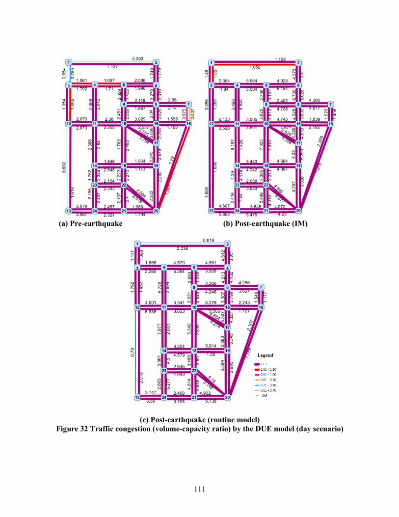
111
(a) Pre-earthquake (b) Post-earthquake (IM)
(c) Post-earthquake (routine model) Figure 32 Traffic congestion (volume-capacity ratio) by the DUE model (day scenario)
Legend
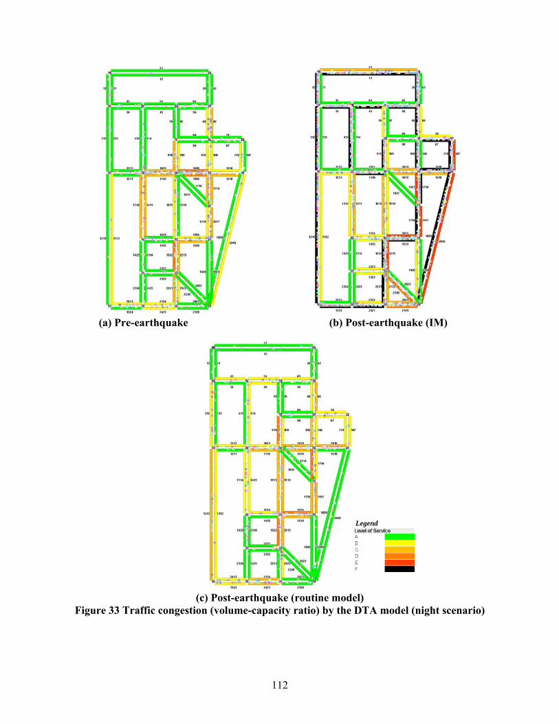
112
(a) Pre-earthquake (b) Post-earthquake (IM)
(c) Post-earthquake (routine model)
Figure 33 Traffic congestion (volume-capacity ratio) by the DTA model (night scenario)
Legend
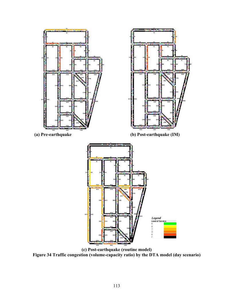
113
(a) Pre-earthquake (b) Post-earthquake (IM)
(c) Post-earthquake (routine model)
Figure 34 Traffic congestion (volume-capacity ratio) by the DTA model (day scenario)
Legend
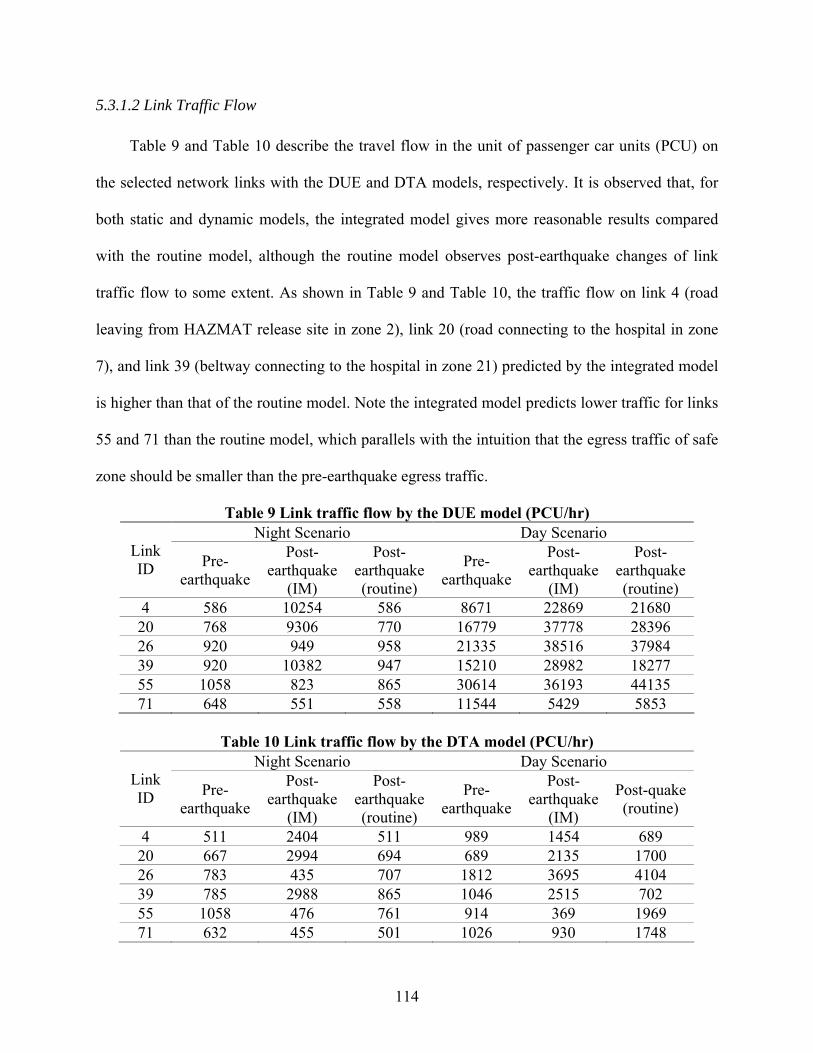
114
5.3.1.2 Link Traffic Flow
Table 9 and Table 10 describe the travel flow in the unit of passenger car units (PCU) on
the selected network links with the DUE and DTA models, respectively. It is observed that, for
both static and dynamic models, the integrated model gives more reasonable results compared
with the routine model, although the routine model observes post-earthquake changes of link
traffic flow to some extent. As shown in Table 9 and Table 10, the traffic flow on link 4 (road
leaving from HAZMAT release site in zone 2), link 20 (road connecting to the hospital in zone
7), and link 39 (beltway connecting to the hospital in zone 21) predicted by the integrated model
is higher than that of the routine model. Note the integrated model predicts lower traffic for links
55 and 71 than the routine model, which parallels with the intuition that the egress traffic of safe
zone should be smaller than the pre-earthquake egress traffic.
Table 9 Link traffic flow by the DUE model (PCU/hr) Night Scenario Day Scenario
Link ID Pre-
earthquake
Post-earthquake
(IM)
Post-earthquake (routine)
Pre-earthquake
Post-earthquake
(IM)
Post-earthquake (routine)
4 586 10254 586 8671 22869 21680 20 768 9306 770 16779 37778 28396 26 920 949 958 21335 38516 37984 39 920 10382 947 15210 28982 18277 55 1058 823 865 30614 36193 44135 71 648 551 558 11544 5429 5853
Table 10 Link traffic flow by the DTA model (PCU/hr)
Night Scenario Day Scenario Link ID Pre-
earthquake
Post-earthquake
(IM)
Post-earthquake (routine)
Pre-earthquake
Post-earthquake
(IM)
Post-quake (routine)
4 511 2404 511 989 1454 689 20 667 2994 694 689 2135 1700 26 783 435 707 1812 3695 4104 39 785 2988 865 1046 2515 702 55 1058 476 761 914 369 1969 71 632 455 501 1026 930 1748
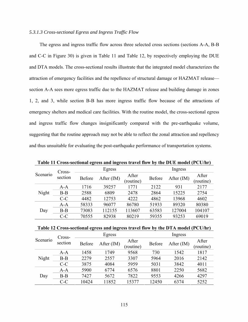
115
5.3.1.3 Cross-sectional Egress and Ingress Traffic Flow
The egress and ingress traffic flow across three selected cross sections (sections A-A, B-B
and C-C in Figure 30) is given in Table 11 and Table 12, by respectively employing the DUE
and DTA models. The cross-sectional results illustrate that the integrated model characterizes the
attraction of emergency facilities and the repellence of structural damage or HAZMAT release—
section A-A sees more egress traffic due to the HAZMAT release and building damage in zones
1, 2, and 3, while section B-B has more ingress traffic flow because of the attractions of
emergency shelters and medical care facilities. With the routine model, the cross-sectional egress
and ingress traffic flow changes insignificantly compared with the pre-earthquake volume,
suggesting that the routine approach may not be able to reflect the zonal attraction and repellency
and thus unsuitable for evaluating the post-earthquake performance of transportation systems.
Table 11 Cross-sectional egress and ingress travel flow by the DUE model (PCU/hr)
Egress Ingress Scenario
Cross-section Before After (IM)
After (routine)
Before After (IM) After
(routine) A-A 1716 39257 1771 2122 931 2177 B-B 2588 6809 2478 2864 15225 2754 Night C-C 4482 12753 4222 4862 13968 4602 A-A 58333 96077 86780 51933 89320 80380 B-B 73083 112155 113607 63583 127004 104107 Day C-C 70555 82938 80219 59355 93253 69019
Table 12 Cross-sectional egress and ingress travel flow by the DTA model (PCU/hr)
Egress Ingress Scenario
Cross-section Before After (IM)
After (routine)
Before After (IM) After
(routine) A-A 1458 1749 9568 730 1542 1817 B-B 2279 2557 3307 5964 2016 2142 Night C-C 3875 4084 5959 5031 3842 4011 A-A 5900 6774 6576 8801 2250 5682 B-B 7427 5672 7822 9553 4266 4297 Day C-C 10424 11852 15377 12450 6374 5252
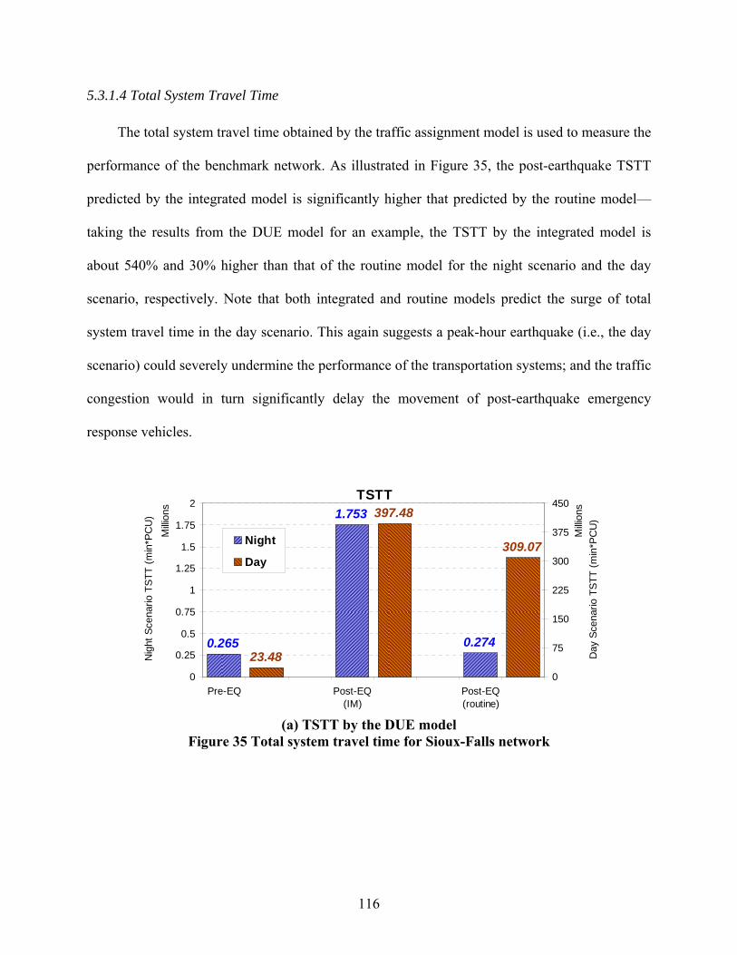
116
5.3.1.4 Total System Travel Time
The total system travel time obtained by the traffic assignment model is used to measure the
performance of the benchmark network. As illustrated in Figure 35, the post-earthquake TSTT
predicted by the integrated model is significantly higher that predicted by the routine model—
taking the results from the DUE model for an example, the TSTT by the integrated model is
about 540% and 30% higher than that of the routine model for the night scenario and the day
scenario, respectively. Note that both integrated and routine models predict the surge of total
system travel time in the day scenario. This again suggests a peak-hour earthquake (i.e., the day
scenario) could severely undermine the performance of the transportation systems; and the traffic
congestion would in turn significantly delay the movement of post-earthquake emergency
response vehicles.
TSTT
0.265
1.753
0.27423.48
397.48
309.07
0
0.25
0.5
0.75
1
1.25
1.5
1.75
2
Pre-EQ Post-EQ(IM)
Post-EQ(routine)
Mill
ions
Nig
ht S
cena
rio T
ST
T (
min
*PC
U)
0
75
150
225
300
375
450
Mill
ions
Day
Sce
nario
TS
TT
(m
in*P
CU
)
Night
Day
(a) TSTT by the DUE model
Figure 35 Total system travel time for Sioux-Falls network
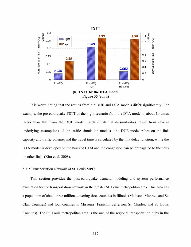
117
TSTT
0.039
0.209
0.052
0.59
1.301.33
0
0.05
0.1
0.15
0.2
0.25
0.3
Pre-EQ Post-EQ(IM)
Post-EQ(routine)
Mill
ions
Nig
ht S
cena
rio T
ST
T (
min
*PC
U)
0
0.2
0.4
0.6
0.8
1
1.2
1.4
Mill
ions
Day
Sce
nario
TS
TT
(m
in*P
CU
)Night
Day
(b) TSTT by the DTA model
Figure 35 (cont.)
It is worth noting that the results from the DUE and DTA models differ significantly. For
example, the pre-earthquake TSTT of the night scenario from the DTA model is about 10 times
larger than that from the DUE model. Such substantial dissimilarities result from several
underlying assumptions of the traffic simulation models—the DUE model relies on the link
capacity and traffic volume, and the travel time is calculated by the link delay function; while the
DTA model is developed on the basis of CTM and the congestion can be propagated to the cells
on other links (Kim et al. 2008).
5.3.2 Transportation Network of St. Louis MPO
This section provides the post-earthquake demand modeling and system performance
evaluation for the transportation network in the greater St. Louis metropolitan area. This area has
a population of about three million, covering three counties in Illinois (Madison, Monroe, and St.
Clair Counties) and four counties in Missouri (Franklin, Jefferson, St. Charles, and St. Louis
Counties). The St. Louis metropolitan area is the one of the regional transportation hubs in the

118
Mid-west U.S. as well as the home of the second-largest inland port by trip ton-miles and the
third-largest rail center in the U.S. (St. Louis RCGA n.d.).
The road network data for the St. Louis metropolitan area, including the locations of
network node and link, road characteristics, and OD travel demand are collected from the local
MPO—the East-West Gateway Council of Governments. The St. Louis network consists of
17352 nodes, 40432 links, and 7263025 OD pairs are defined for the network. The OD demand
during the AM and OP periods is taken as the “background” traffic for the morning scenario and
night scenario, respectively. There are a total number of 3962 bridges on the St. Louis network,
as documented in the 2002 Nation Bridge Inventory. Figure 36 shows the transportation network
and bridges in the St. Louis study area. This study conducts the seismic performance assessment
of the St. Louis MPO network on the basis of the NMSZ M7.7 scenario earthquake as described
in Section 3.2. Figure 37 shows the PGA map for the study region and the bridge functionalities
at day 0 under the NMSZ scenario earthquake.
The zonal traffic generation for each TAZ is based on its trip attraction and trip production,
following the procedures described in Section 5.2.2.1. In this study, the general building
inventory is taken from the default building inventory of HAZUS-MH MR2 and MR3. Inventory
of essential facilities is taken from the 2008 Homeland Security Infrastructure Program (HSIP)
dataset and the American Red Cross National Shelter System (NSS), including schools and
colleges, hospitals, correctional facilities, and emergency shelters. Structural damage to general
building stock (at census tract level) and essential facilities (at individual facility level) are taken
from the assessment results from the MAE Center’s seismic impact assessment for the Central
United States (Elnashai et al. 2009).
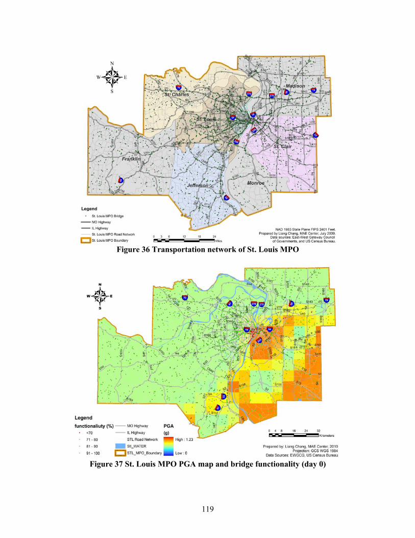
119
Figure 36 Transportation network of St. Louis MPO
Figure 37 St. Louis MPO PGA map and bridge functionality (day 0)
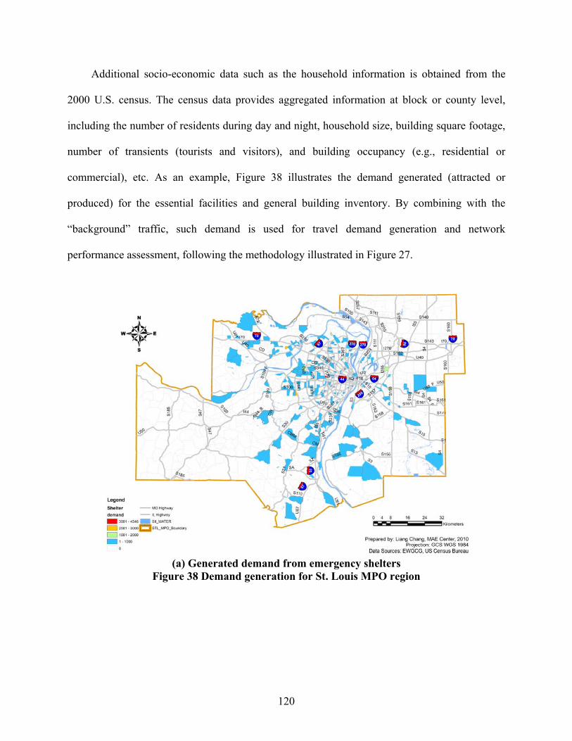
120
Additional socio-economic data such as the household information is obtained from the
2000 U.S. census. The census data provides aggregated information at block or county level,
including the number of residents during day and night, household size, building square footage,
number of transients (tourists and visitors), and building occupancy (e.g., residential or
commercial), etc. As an example, Figure 38 illustrates the demand generated (attracted or
produced) for the essential facilities and general building inventory. By combining with the
“background” traffic, such demand is used for travel demand generation and network
performance assessment, following the methodology illustrated in Figure 27.
(a) Generated demand from emergency shelters
Figure 38 Demand generation for St. Louis MPO region
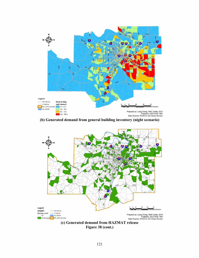
121
(b) Generated demand from general building inventory (night scenario)
(c) Generated demand from HAZMAT release
Figure 38 (cont.)
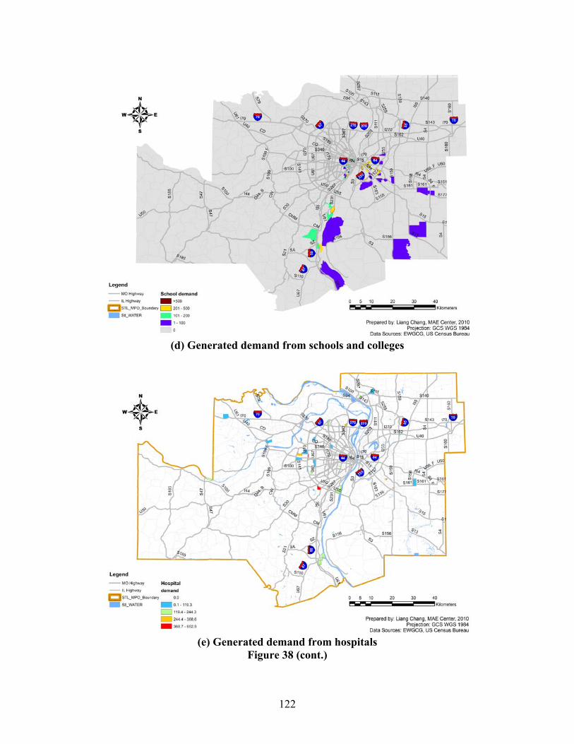
122
(d) Generated demand from schools and colleges
(e) Generated demand from hospitals
Figure 38 (cont.)
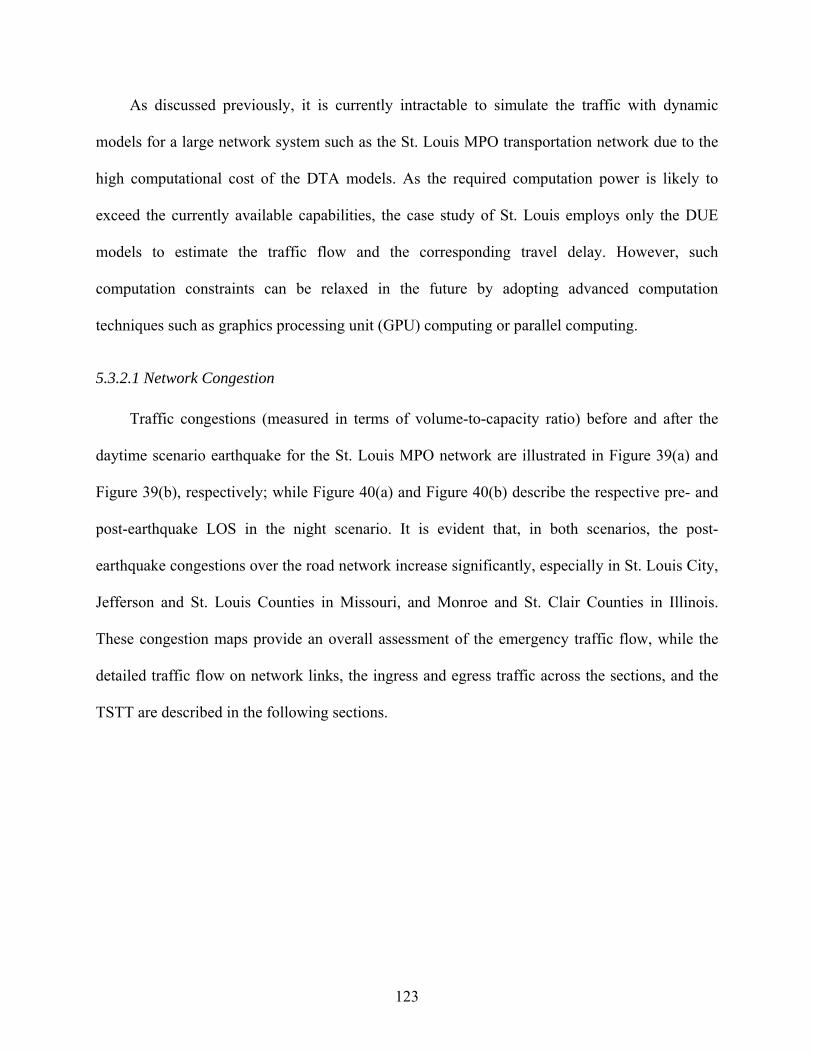
123
As discussed previously, it is currently intractable to simulate the traffic with dynamic
models for a large network system such as the St. Louis MPO transportation network due to the
high computational cost of the DTA models. As the required computation power is likely to
exceed the currently available capabilities, the case study of St. Louis employs only the DUE
models to estimate the traffic flow and the corresponding travel delay. However, such
computation constraints can be relaxed in the future by adopting advanced computation
techniques such as graphics processing unit (GPU) computing or parallel computing.
5.3.2.1 Network Congestion
Traffic congestions (measured in terms of volume-to-capacity ratio) before and after the
daytime scenario earthquake for the St. Louis MPO network are illustrated in Figure 39(a) and
Figure 39(b), respectively; while Figure 40(a) and Figure 40(b) describe the respective pre- and
post-earthquake LOS in the night scenario. It is evident that, in both scenarios, the post-
earthquake congestions over the road network increase significantly, especially in St. Louis City,
Jefferson and St. Louis Counties in Missouri, and Monroe and St. Clair Counties in Illinois.
These congestion maps provide an overall assessment of the emergency traffic flow, while the
detailed traffic flow on network links, the ingress and egress traffic across the sections, and the
TSTT are described in the following sections.
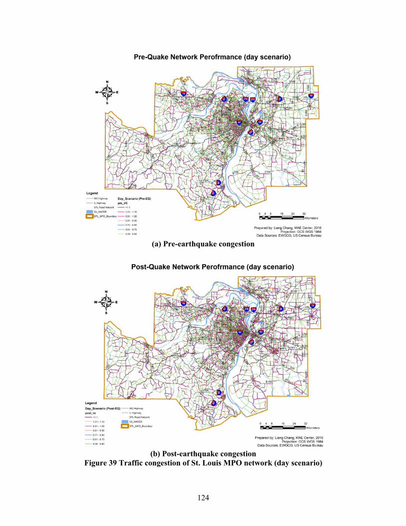
124
(a) Pre-earthquake congestion
(b) Post-earthquake congestion
Figure 39 Traffic congestion of St. Louis MPO network (day scenario)
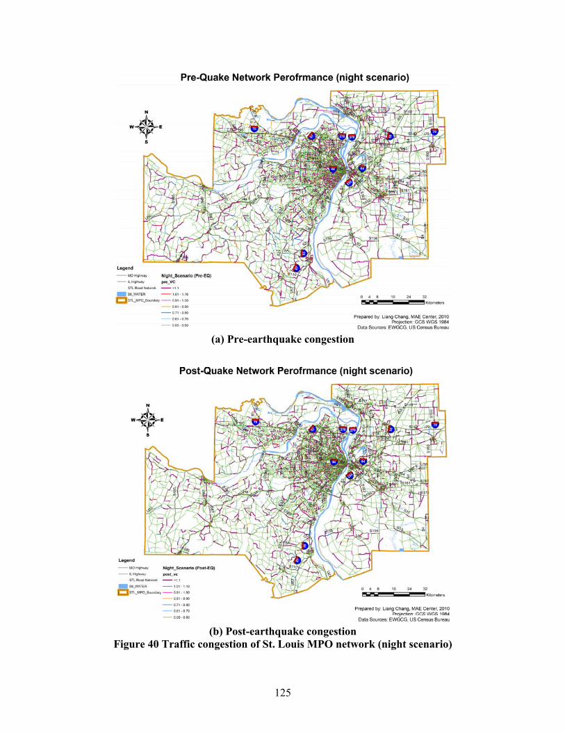
125
(a) Pre-earthquake congestion
(b) Post-earthquake congestion
Figure 40 Traffic congestion of St. Louis MPO network (night scenario)
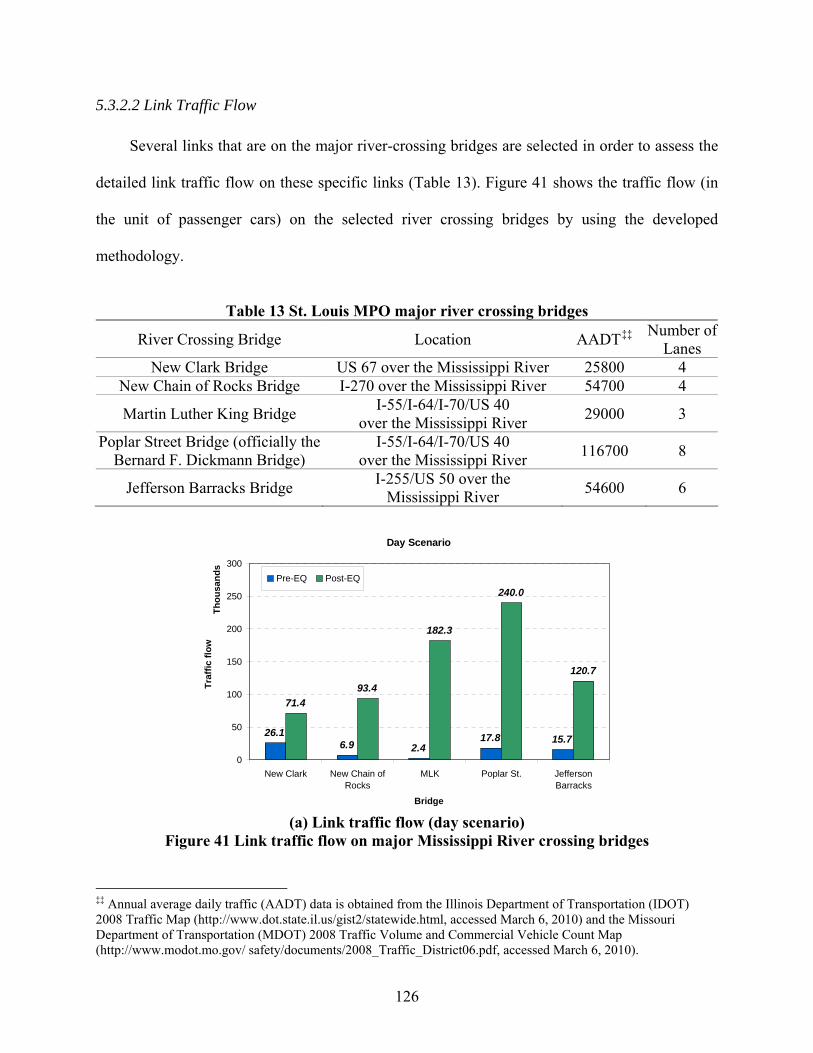
126
5.3.2.2 Link Traffic Flow
Several links that are on the major river-crossing bridges are selected in order to assess the
detailed link traffic flow on these specific links (Table 13). Figure 41 shows the traffic flow (in
the unit of passenger cars) on the selected river crossing bridges by using the developed
methodology.
Table 13 St. Louis MPO major river crossing bridges
River Crossing Bridge Location AADT‡‡ Number of
Lanes New Clark Bridge US 67 over the Mississippi River 25800 4
New Chain of Rocks Bridge I-270 over the Mississippi River 54700 4
Martin Luther King Bridge I-55/I-64/I-70/US 40
over the Mississippi River 29000 3
Poplar Street Bridge (officially the Bernard F. Dickmann Bridge)
I-55/I-64/I-70/US 40 over the Mississippi River
116700 8
Jefferson Barracks Bridge I-255/US 50 over the
Mississippi River 54600 6
Day Scenario
6.9 2.417.8 15.7
71.4
93.4
182.3
240.0
120.7
26.1
0
50
100
150
200
250
300
New Clark New Chain ofRocks
MLK Poplar St. JeffersonBarracks
Th
ou
san
ds
Bridge
Tra
ffic
flo
w
Pre-EQ Post-EQ
(a) Link traffic flow (day scenario)
Figure 41 Link traffic flow on major Mississippi River crossing bridges
‡‡ Annual average daily traffic (AADT) data is obtained from the Illinois Department of Transportation (IDOT) 2008 Traffic Map (http://www.dot.state.il.us/gist2/statewide.html, accessed March 6, 2010) and the Missouri Department of Transportation (MDOT) 2008 Traffic Volume and Commercial Vehicle Count Map (http://www.modot.mo.gov/ safety/documents/2008_Traffic_District06.pdf, accessed March 6, 2010).
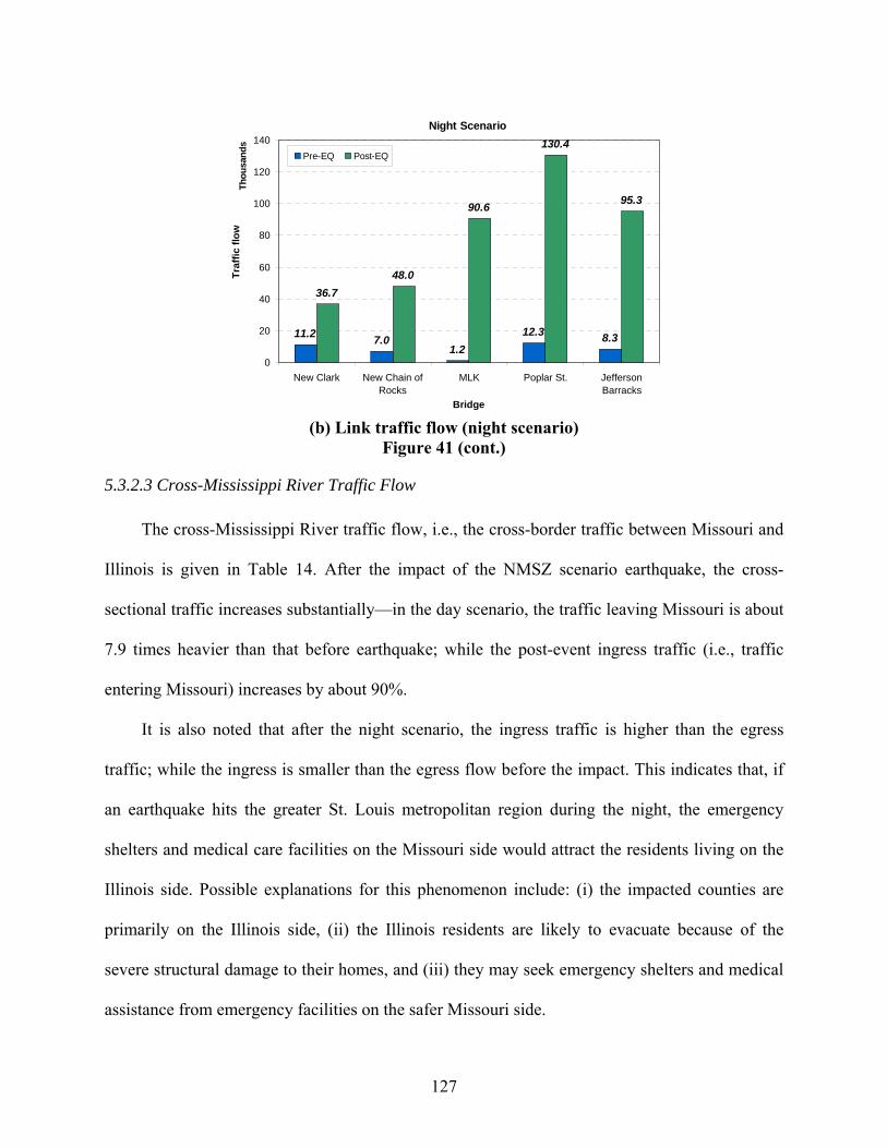
127
Night Scenario
11.27.0
1.2
12.3 8.3
36.7
48.0
90.6
130.4
95.3
0
20
40
60
80
100
120
140
New Clark New Chain ofRocks
MLK Poplar St. JeffersonBarracks
Th
ou
san
ds
Bridge
Tra
ffic
flo
w
Pre-EQ Post-EQ
(b) Link traffic flow (night scenario)
Figure 41 (cont.)
5.3.2.3 Cross-Mississippi River Traffic Flow
The cross-Mississippi River traffic flow, i.e., the cross-border traffic between Missouri and
Illinois is given in Table 14. After the impact of the NMSZ scenario earthquake, the cross-
sectional traffic increases substantially—in the day scenario, the traffic leaving Missouri is about
7.9 times heavier than that before earthquake; while the post-event ingress traffic (i.e., traffic
entering Missouri) increases by about 90%.
It is also noted that after the night scenario, the ingress traffic is higher than the egress
traffic; while the ingress is smaller than the egress flow before the impact. This indicates that, if
an earthquake hits the greater St. Louis metropolitan region during the night, the emergency
shelters and medical care facilities on the Missouri side would attract the residents living on the
Illinois side. Possible explanations for this phenomenon include: (i) the impacted counties are
primarily on the Illinois side, (ii) the Illinois residents are likely to evacuate because of the
severe structural damage to their homes, and (iii) they may seek emergency shelters and medical
assistance from emergency facilities on the safer Missouri side.
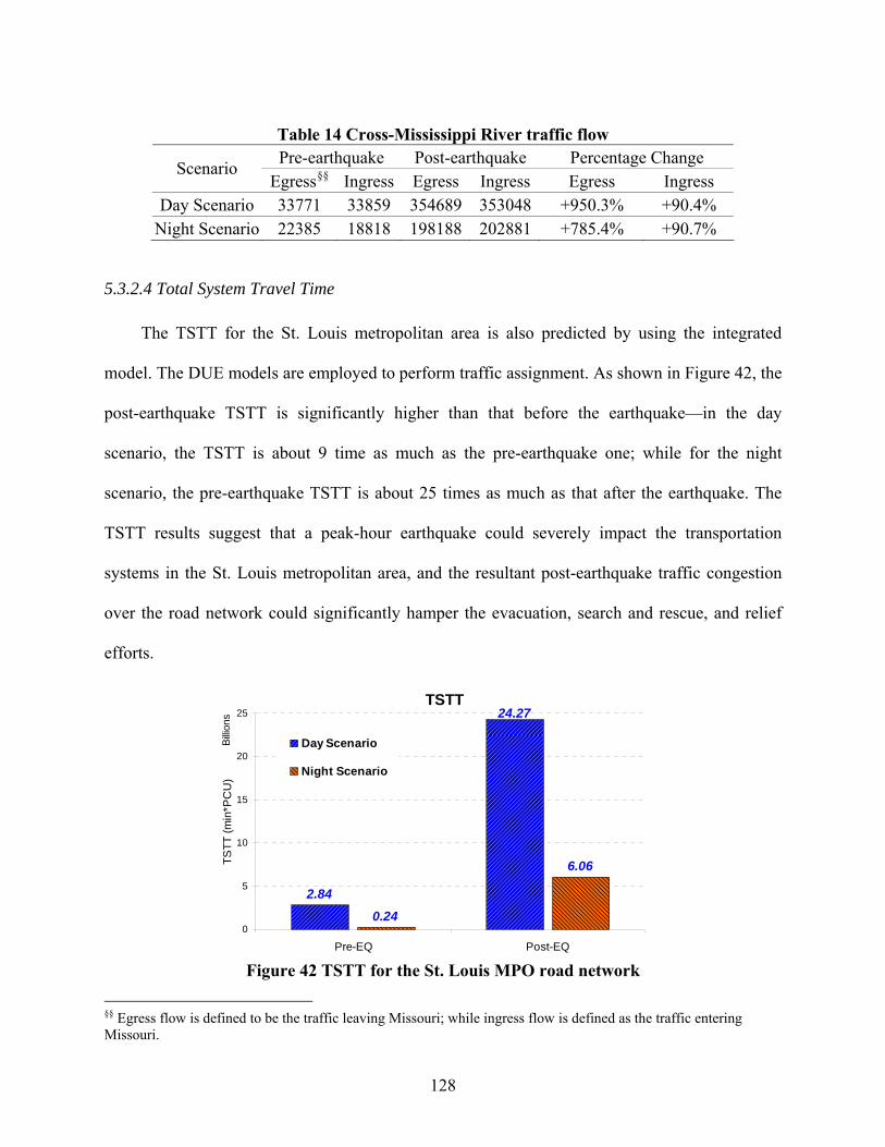
128
Table 14 Cross-Mississippi River traffic flow Pre-earthquake Post-earthquake Percentage Change
Scenario Egress§§ Ingress Egress Ingress Egress Ingress
Day Scenario 33771 33859 354689 353048 +950.3% +90.4% Night Scenario 22385 18818 198188 202881 +785.4% +90.7%
5.3.2.4 Total System Travel Time
The TSTT for the St. Louis metropolitan area is also predicted by using the integrated
model. The DUE models are employed to perform traffic assignment. As shown in Figure 42, the
post-earthquake TSTT is significantly higher than that before the earthquake—in the day
scenario, the TSTT is about 9 time as much as the pre-earthquake one; while for the night
scenario, the pre-earthquake TSTT is about 25 times as much as that after the earthquake. The
TSTT results suggest that a peak-hour earthquake could severely impact the transportation
systems in the St. Louis metropolitan area, and the resultant post-earthquake traffic congestion
over the road network could significantly hamper the evacuation, search and rescue, and relief
efforts.
TSTT
0.24
6.06
2.84
24.27
0
5
10
15
20
25
Pre-EQ Post-EQ
Bill
ions
TS
TT
(m
in*P
CU
)
Day Scenario
Night Scenario
Figure 42 TSTT for the St. Louis MPO road network
§§ Egress flow is defined to be the traffic leaving Missouri; while ingress flow is defined as the traffic entering Missouri.
129
5.4. Summary
This chapter develops a travel demand modeling methodology to simulate the post-
earthquake performance of transportation systems. The post-earthquake changes of travel
behavior are taken into account by using the integrated methodology, which approximates the
“abnormal” travel demand and simulates the post-earthquake traffic by considering the damage
of bridge and building structures, HAZMAT releases, and the “attraction” of essential emergency
facilities. Several major assumptions on evacuation behavior and post-earthquake traffic
management measures are made to simplify the complex problem of demand modeling in
extreme events.
The proposed methodology is demonstrated with two case studies—the Sioux-Falls road
network and the transportation network in the greater St. Louis metropolitan area. The
performance of transportation systems is evaluated under two hypothetical scenarios that
characterize the distinct post-earthquake traffic patterns at different times. The traffic flow and
travel cost are identified to help evaluate the emergency performance of transportation systems.
The findings from the numerical case studies suggest that: (i) an earthquake occurring
during peak hours would severely impact the transportation systems and result in significant
delays and congestion, (ii) by accounting for the effects of emergency facilities and the post-
earthquake changes of travel behavior and route choices, the integrated methodology can capture
the “abnormal” travel patterns and give more reasonable results than the conventional
approaches.
The proposed methodology can be combined with the OD-independent performance
metrics to aid emergency managers and traffic planner to evaluate their contingency plans for
emergency training, preparedness, and response.
130
CHAPTER VI CONCLUSIONS AND FUTURE RESEARCH
In this chapter summaries of the major conclusions are given. Also discussion of future
work on risk assessment and disaster management of transportation systems in the context of
earthquake engineering is given.
6.1 Conclusions
The goal of this dissertation was to develop a systematic methodology to model risk from
catastrophic events, explore the performance and disaster resiliencies for transportation
infrastructure systems, and provide decision support tools for emergency management. The
above objectives were accomplished by developing an approach for evaluating the performance
of transportation systems and providing effective intervention strategies to mitigate potential
losses from earthquakes. The major conclusions and contributions from the dissertation are
summarized below.
The travel delay cost-based performance assessment by MAE Center’s existing NBSR
methodology, while important, was found inefficient to identify the optimal solutions for large
infrastructure systems due to excessive computational costs. In addition, the fixed travel demand
model employed by the existing NBSR methodology is not suitable to address the changes of
travel behavior or demand after a disruptive earthquake. Thus, the current NBSR methodology
may lead to an inadequate quantification of the functional loss of the transportation systems.
The applicability of existing NBSR approach was improved by employing OD-independent
performance metrics and efficient optimization techniques, which overcame the limitation of the
unrealistic assumption on post-disaster travel patterns. Results from the extended NBSR revealed
that the effectiveness of retrofit programs increases with the budget but with diminishing returns.

131
In other words, higher budget levels would lead to more effective seismic retrofit programs. It
was also demonstrated that additional retrofitting becomes less effective after the investment
exceeds a critical level of budget.
Furthermore, the reliability of network reachability was efficiently quantified by
implementing the state-of-the-art recursive decomposition algorithm. The reliability of network
reachability was illustrated to be better suited to assisting in the decision making for immediate
post-disaster responses. This performance metric provided essential information of post-
earthquake completeness or connectedness by rapidly identifying the regions that are potentially
difficult to reach after a disruptive earthquake.
The convergence of system performance was tested and the sensitivity to input parameters
(e.g., PGA and MCS sample size) was investigated as well. The discussion of ground motion
correlation provided a better understanding of the effects of spatial ground motion correlation on
the behavior of spatially distributed transportation systems.
Lastly, in order to model the functional loss of transportation systems under emergency
situations, the abnormal post-earthquake travel behavior and the performance of highway
systems were studied. The fixed travel demand models are limited for modeling the post-
earthquake transportation systems due to the unrealistic travel demand assumptions. An
integrated demand simulation model was developed to incorporate the traffic pattern changes
after a damaging earthquake.
The established assumptions on travelers’ post-earthquake behavior and traffic management
measures helped to approximate the complex demand modeling process. The structural damage
of bridge and building structures, HAZMAT releases, and the attraction of essential emergency
facilities were taken into account in the developed post-earthquake demand model. The
132
discussion on trip generation for different zone types provided an effective characterization of
the effects of attractants (i.e., hospitals and emergency shelters) and repellents (i.e., HAZMAT
release and structural damage) on the post-earthquake traffic modeling. Furthermore, this
research introduced two hypothetical scenarios that postulate and model the effects of a no-
notice earthquake event on transportation systems. By extending the conventional four-step
UTPP approach, the post-earthquake travel demand was established with the integrated trip
distribution/assignment model. Subsequently, the post-earthquake functional loss of
transportation systems was assessed by loading the generated “abnormal” demand to the
damaged transportation network with traffic simulation models.
The developed demand modeling methodology was illustrated by the Sioux-Falls network
as a numerical case study. Both DUE and DTA were applied in this case study and the results
consistently demonstrated that: (i) the earthquake occurrence time significantly influenced the
level and spatial distribution of traffic congestion—an earthquake happening during peak hours
would severely impact the transportation systems and cause significant delays and congestion;
and (ii) compared with the routine demand models, the integrated model captured the
“abnormal” traffic patterns and provided more reasonable results (i.e., link traffic flow,
congestion levels, spatial distribution of the congested areas, and TSTT) by accounting for the
effects of emergency facilities and travelers’ behavior changes.
Transportation systems in the St. Louis metropolitan area were studied to evaluate their
post-earthquake functionality by using the integrated model. The post-earthquake travel demand
was generated for the St. Louis MPO network based on MAE Center’s seismic impact
assessment of the general building inventory and essential facilities.
133
The output of these case studies proved that the integrated demand modeling methodology
is very helpful to model the post-earthquake functionality of transportation systems—it provided
an effective scenario-based means to characterize zonal trip generation by accounting for the
attractants and repellents during the period of emergency response.
In brief, the developed methodologies allow state and local authorities and emergency
managers to:
model catastrophe risks, evaluate post-earthquake physical damage, and assess the
performance and functionality of critical transportation infrastructures such as
system reliability and disaster resiliencies, for sustainable growth;
support decision-making in infrastructure project planning, construction, operation,
and renewal by identifying strategic budget and mitigation priority for future
extreme events;
assess the contingency plans for emergency training and response, secure the critical
ingress and egress routes for emergency response as well as avoid excessive queues
and delays.
This research can also be extended to incorporate damages to other network components
(e.g., roadway segments) and include other types of man-made and natural hazards such as
intentional attacks and hurricanes without changing the methodological framework.
6.2 Future Research
The risk assessment and modeling of transportation infrastructure systems covers a broad
spectrum of research areas and only some of the components were studied in detail in this
research. The limitations of this research require additional research in the future, especially in
the topics given below.
134
The details of the developed methodologies were developed specifically for road networks
subjected to earthquakes. The study did not take into account other natural or man-made hazards.
In the future, resiliencies of transportation infrastructure systems needs to be evaluated under the
exposure to multiple environmental hazards or intentional disturbances (e.g., hurricane or
intentional attack) for a comprehensive catastrophe risk modeling and systematic assessment of
civil infrastructure systems. Furthermore, fire following earthquake will be a major issue for
many parts of the Midwest U.S. with densely spaced wood buildings. Evacuated population due
to fires following earthquake needs to be included to accurately model the post-earthquake travel
demand and the performance of transportation systems.
Because bridges are particularly vulnerable in the transportation system, this research
assumed the bridges are the only vulnerable components of transportation systems. However,
vulnerability of other transportation network components should be addressed in future research.
For example, roadways are particularly vulnerable to earthquakes due to liquefaction or surface
fault rupture. The relationship between roadway damage and intensities of ground shaking,
however, is relatively little known in the literature. The quality of modeling and assessment for
transportation system would benefit from the consideration of vulnerabilities of other
components.
Validation of the developed methodologies was not performed in this research because of
the insufficient data from the rare NMSZ earthquakes. Furthermore, the post-earthquake traffic
patterns are transient and such data is difficult to collect in a timely manner. Nevertheless,
validation efforts should be emphasized in future studies to calibrate the developed approaches
by collecting the post-earthquake traffic data with the emerging technologies such as GPS-
enabled mobile phones.

135
In this research, the interdependencies between the transportation systems and other urban
infrastructure networks such as power grids were not discussed. Though urban infrastructure
systems are built and operated as stand-alone entities, in actuality they are highly interconnected
and functionally interdependent—power outage-caused traffic signal failure would result in
elongated travel delay, which in turn would hinder the recovery of power grids. Recognition of
the interdependencies among critical infrastructure systems could promote a better understanding
of the links between infrastructure systems in the dynamic built environment. Further research
would be beneficial to better understand the impact of interdependencies among critical
infrastructure on their robustness and resiliencies.
136
REFERENCES
Abrahamson, N. A., and Youngs, R. R. (1992). “A stable algorithm for regression analyses using the random effects model.” Bulletin of the Seismological Society of America, 82(1), 505-510.
Adachi, T., and Ellingwood, B. (2007). “Impact of infrastructure interdependency and spatial correlation of seismic intensities on performance assessment of a water distribution system.” Proceedings of the 10th International Conference on Applications of Statistics and Probability in Civil Engineering (ICASP10), Taylor & Francis, New York, NY.
Aggarwal, K. K., and Misra, K. B. (1975). “A fast algorithm for reliability evaluation.” IEEE Transactions on Reliability, 24(1), 83-85.
Ahmad, S. H. (1982). “A simple technique for computing network reliability.” IEEE Transactions on Reliability, R-31(1), 41-44.
Ahuja, R. K., Magnanti, T. L., and Orlin, J. B. (1993). Network flows: Theory, algorithms, and applications, Prentice Hall Press, Upper Saddle River, NJ.
Alexander, D. (2002). Principles of emergency planning and management, 3rd Ed., Oxford University Press, New York, NY.
American Society of Civil Engineers (ASCE) (2009). “Report card for America’s infrastructure.” <http://www.infrastructurereportcard.org/fact-sheet/bridges> (June 5, 2009).
Anil, M., and Ozbay, K. (2007). “Impact of probabilistic road capacity constraints on the spatial distribution of hurricane evacuation shelter capacities.” Transportation Research Record: Journal of the Transportation Research Board, 2022, 55-62.
Applied Technology Council (ATC) (1985). Earthquake damage evaluation data for California (ATC-13), ATC, Redwood City, CA.
ATC. (1983). Seismic retrofitting guidelines for highway bridges (ATC-6-2), ATC, Palo Alto, CA.
ATC. (1991). Seismic vulnerability and impact of disruption of lifelines in the conterminous United States (ATC-25), ATC, Redwood City, CA.
Ardekani, S. A. (1992a). “Transportation operations following the 1989 Loma Prieta earthquake.” Transportation Quarterly, 46(2), 219-233.
Ardekani, S. A. (1992b). “A decision tool for transportation operations following urban disasters.” Final Report to Earthquake Hazard Mitigation Program, National Science Foundation (Grant No. BCS-9005042). Department of Civil Engineering, University of Texas at Arlington, Arlington, Texas.
137
Ardekani, S. A. (1995). “Post-quake transportation operations following the 1994 Northridge earthquake.” Proceedings of the 4th U.S. Conference on Lifeline Earthquake Engineering, TCLEE Monograph No. 6, ASCE, Reston, VA.
Ashford, S. A., and Kawamata, Y. (2006). “Performance of transportation systems during the 2004 Niigata Ken Chuetsu, Japan, Earthquake.” Earthquake Spectra, 22(S1), S111-S132.
Augusti, G., Borri, A., and Ciampoli, M. (1994). “Optimal allocation of resources in reduction of the seismic risks of a highway network.” Engineering Structures, 16(7), 485-497.
Baker, E. J. (1991). “Hurricane evacuation behavior.” International Journal of Mass Emergencies and Disasters, 9(2), 287-310.
Bana e Costa, C. A., Oliveira, C. S., and Vieira, V. (2008). “Prioritization of bridges and tunnels in earthquake risk mitigation using multicriteria decision analysis: Application to Lisbon.” OMEGA: The International Journal of Management Science, 36(3), 442-450.
Bao. Y., and Li, J. (2004). “A comparison research on the methods of analyzing lifeline systems’ seismic reliability.” Journal of Disaster Prevention and Mitigation Engineering (Fang Zai Jian Zai Gong Cheng Xue Bao), 24(2), 139-148.
Barton-Aschman and Associates. (1994). 1994 Northridge Earthquake Recovery, Interim Report No. 1. California Department of Transportation District 7, Los Angeles, CA.
Basőz, N., and Kiremidjian, A. S. (1996). Risk assessment for highway systems, Report No. 118, John A. Blume Earthquake Engineering Center, Department of Civil Engineering, Stanford University, Stanford, CA.
Basőz, N., Kiremidjian, A. S., King, S. A., and Law, K. H. (1999). “Statistical analysis of bridge damage data from the 1994 Northridge, CA, Earthquake.” Earthquake Spectra, 15(1), 25-54.
Beckmann, M., McGuire, C. B., and Winsten, C. B. (1956). Studies in the economics of transportation, Yale University Press, New Haven, CT.
Ben-Akiva, M. E., Koutsopoulos, H. N., Mishalani, R., and Yang, Q. (1997) “Simulation laboratory for evaluating dynamic traffic management systems.” ASCE Journal of Transportation Engineering, 123(4), 283-289.
Boarnet, M. G. (1996). Business losses, transportation damage and the Northridge Earthquake, Paper No. 341, University of California Transportation Center, Berkeley, CA.
Bommer, J., and Crowley, H. (2006). “The influence of ground-motion variability in earthquake loss modelling.” Bulletin of Earthquake Engineering, 4(3), 231-248.
Boore, D. M. (2003). “Simulation of ground motion using the stochastic method.” Pure and Applied Geophysics, 160(3), 635-676.
138
Boyce, D., Lee, D., and Ran, B. (2001). “Analytical models of the dynamic traffic assignment problem.” Networks and Spatial Economics, 1, 377-309.
Buckle, I. G., and Copper, J. D. (1995). “Mitigation of seismic damage to lifelines: Highways and railroads.” Critical issues and state-of-the-art in lifeline earthquake engineering, TCLEE Monograph No. 7, ASCE, Reston, VA.
Burdette, N. J., and Elnashai, A. S. (2008). “Effect of asynchronous earthquake motion on complex bridges. II: Results and implications on assessment.” Journal of Bridge Engineering, 13(2), 166-172.
Burdette, N. J., Elnashai, A. S., Lupoi, A., and Sextos, A. G. (2008). “Effect of asynchronous earthquake motion on complex bridges. I: methodology and input motion.” Journal of Bridge Engineering, 13(2), 158-165.
Bureau of Transportation Statistics (BTS) (2005). “The 2002 commodity flow survey.” <http://www.bts.gov/publications/commodity_flow_survey/index.html> (May 2, 2006).
California Department of Transportation (Caltrans) (1995). Northridge earthquake recovery: Final comprehensive transportation analysis, Caltrans District 7, Division of Operation, Los Angeles, CA.
Campbell, K. W. (1985). “Strong motion attenuation relations: A ten-year perspective.” Earthquake Spectra, 1(4), 759-804.
Campbell, K. W., and Bozorgnia, Y. (2007). “Campbell-Bozorgnia NGA ground motion relations for the geometric horizontal component of peak and spectral ground motion parameters.” Pacific Earthquake Engineering Research Center Report (No. 2007/02). University of California, Berkeley, CA.
Carey, M. (1986). “A constraint qualification for a dynamic traffic assignment model.” Transportation Science, 20(1), 55-58.
Carey, M. (1987). “Optimal time-varying flows on congested networks.” Operations Research, 35(1), 58-69.
Carey, M. (1992). “Nonconvexity of the dynamic traffic assignment problem.” Transportation Research, 26B(2), 127-133.
Central United States Earthquake Consortium (CUSEC) (2000). “Earthquake vulnerability of transportation systems in the Central United States.” <http://cusec.org/publications/ brochures/dotmonograph.pdf> (January 16, 2008).
Chang, E. C. (2003). Traffic simulation for effective emergency evacuation, Oak Ridge National Laboratory, Oak Ridge, TN.
139
Chang, L., and Song, J. (2006). “Systematic treatment of uncertainty in consequence-based management of seismic regional losses.” Mid-America Earthquake Center Report < https://www.ideals.uiuc.edu/handle/2142/5124 > (September 9, 2009).
Chang, L., and Song, J. (2007). “Matrix-based system reliability analysis of urban infrastructure networks: A case study of MLGW natural gas network.” The 5th China-Japan-US Trilateral Symposium on Lifeline Earthquake Engineering, X. Zhou, Y. Tanaka, and J. Bardet, eds., Beijing University of technology, Beijing, China.
Chang, L., Elnashai, A. S., and Spencer, B. F. 2009. “Modeling post-earthquake emergency travel demand.” Asian-Pacific Network of Centers for Earthquake Engineering Research (ANCER) Workshop, ANCER, Urbana, IL.
Chang, L., Peng, F., Ouyang, Y., Elnashai, A. S., and Spencer, B. F. (2009). “Strategic budget planning for seismic retrofit of bridge networks.” Transportation Research Board (TRB) 88th Annual Meeting, TRB, Washington, D.C.
Chang, S. E., and Nojima, N. (1998). “Measuring lifeline system performance: Highway transportation system in recent earthquakes.” Proceedings of the 6th National Earthquake Conference on Earthquake Engineering, Paper No. 70, Earthquake Engineering Research Institute (EERI), Oakland, CA.
Chang, S., Shinozuka, M., and Moore, J. (2000). “Probabilistic earthquake scenarios: Extending risk analysis methodologies to spatial distributed systems.” Earthquake Spectra, 16(3), 557-572.
Chatterjee, A., and Venigalla, M. M. (2004). “Travel demand forecasting for urban transportation planning.” Handbook of Transportation Engineering, M. Kutz, ed., McGraw-Hill, New York, NY.
Chen, Y., and Tzeng, G. (1999). “A fuzzy multi-objective model for reconstructing the post-quake road-network by genetic algorithm.” International Journal of Fuzzy Systems, 1(2), 85-95.
Chiu, Y.-C., Korada, P., and Mirchandani, P. B. (2005). “Dynamic traffic management for evacuation.” Transportation Research Board 2005 Annual Meeting, TRB, Washington, D.C.
Choi, E., DesRoches, R., and Nielson, B. (2004). “Seismic fragility of typical bridges in moderate seismic zones.” Engineering Structures, 26 (2), 187-199.
Cornell, C. (1968). “Engineering seismic risk analysis.” Bulletin of the Seismological Society of America, 58(5), 1583-1606.
Cramer, C. (2006). “Quantifying the uncertainty in the site amplifying modeling and its effects on site-specific seismic-hazard estimation in the Upper Mississippi Embayment and adjacent areas.” Bulletin of the Seismological Society of America, 96(6), 2008-2020.
140
Cramer, C. (2008). Personal communication, Associate Research Professor, Center for Earthquake Research and Information (CERI), University of Memphis, Memphis, TN, January 3, 2008.
Cutter, S. L. (1996). “Vulnerability to environmental hazards.” Progress in Human Geography, 20(4), 529-539.
Dafermos, S. (1980). “Traffic equilibrium and variational inequalities.” Transportation Science, 14, 42-54.
Daganzo, C. F. (1994). “The cell transmission model: A dynamic representation of highway traffic consistent with the hydrodynamic theory.” Transportation Research, 28B(4), 269-287.
Daganzo, C. F. (1995). “The cell transmission model II: Network traffic.” Transportation Research, 29B(2), 79-93.
Debban, S. (1995). “Innovative traffic management following the 1994 Northridge earthquake.” <http://www.itsdocs.fhwa.dot.gov/JPODOCS/REPTS_TE/1711.pdf>. (March 2, 2009).
Department of Transport (DfT) (2006). “Variable demand modeling-Preliminary assessment procedures (Transportation Analysis Guidance TAG 3.10.1).” <http://www.webtag.org.uk/ webdocuments/3_Expert/10_Variable_Demand_Modelling/3.10.1.htm> (November 1, 2007).
DesRoches, R. (2008). Personal communication, Associate Professor of Civil and Environmental Engineering, Georgia Institute of Technology, Atlanta, GA, November 1, 2008.
DesRoches, R., Padgett, J. E., Elnashai, A. S., Kim, Y. S., and Reed, D. (2006). “MAE Center transportation test bed.” Proceedings of the 8th U.S. National Conference on the Earthquake Engineering, Paper No. 2044, EERI, Oakland, CA.
Ditlevsen, H. A. (1979). “Narrow reliability bounds for structural systems.” Journal of Structural Mechanics, 7(4), 453-472.
Dotson, W. P., and Gobien, J.O. (1979). “A new analysis technique for probability graphs.” IEEE Transactions on Circuits and Systems, 26, 855-865.
Dueñas-Osorio, L., and Vemuru, S. M. (2009). “Cascading failures in complex infrastructure systems.” Structural Safety, 31(2), 157-167.
Duke, C. M. (1981). “An earthquake hazard plan for lifelines.” Lifeline earthquake engineering: The current state of knowledge, ASCE, New York, NY.
Duncan, G. (2008). Personal communication, Director of Maintenance, Tennessee Department of Transportation, Nashville, TN, December 18, 2008.
Dutta, A. (1999). On energy based seismic analysis and design of highway bridges, Ph.D. Dissertation, Department of Civil, Structural, and Environmental Engineering, Buffalo, State University of New York, NY.
141
Earthquake Engineering Research Institute (EERI) (1986). Reducing earthquake hazards: Lessons learned from earthquakes, EERI, Oakland, CA.
Easa, S. M. (1993). “Urban trip distribution in practice. I: Conventional analysis.” Journal of Transportation Engineering, 119(6), 793-815.
East-West Gateway Coordinating Council (EWGCC) (2003). “Household travel survey: Final report of survey results.” <http://www.ewgateway.org/pdffiles/library/trans/ travelsurvey/StLouisFinalAnalysisReport.pdf> (April 28, 2009).
Edmonds, J. and Karp, R. M. (1972). “Theoretical improvements in algorithmic efficiency for network flow problems”. Journal of the Association for Computing Machinery (ACM), 19(2), 248-264.
Eguchi, R. T., Goltz, J. D., Taylor, C. E., Chang, S. E., Flores, P. J., Johnson, L. A, Seligson, H. A., and Blais, N. C. (1998). “Direct economic losses in the Northridge Earthquake: A three-year post-event perspective.” Earthquake Spectra, 14(2), 245-264.
Eguchi, R. T. (1984). “Seismic risk and decision analysis of lifeline systems.” Lifeline earthquake engineering: Performance, design, and construction. J. D. Cooper, ed., ASCE, New York, NY.
Elnashai, A. S., Cleveland, L. J., Jefferson, T., and Harrald, J. (2009). Impact of earthquakes on the Central USA, Mid-America Earthquake Center Report 09-03, University of Illinois at Urbana-Champaign, Urbana, IL.
Elnashai, A. S., Borzi, B., and Vlachos, S. (2004). “Deformation-based vulnerability functions for RC bridges.” Structural Engineering and Mechanics, 17(2), 215-244.
EQE (1989). The October 17, 1989 Loma Prieta Earthquake, EQE Engineering, San Francisco, CA.
EQE (1994). The January 17, 1994 Northridge, California Earthquake: An EQE Summary report, EQE International, San Francisco, CA.
Evans, S. P. (1976). “Derivation and analysis of some models for combining trip distribution and assignment.” Transportation Research, 10(1), 37-57.
Fan, Y. (2003). Optimal routing through stochastic networks, Ph.D. Dissertation, University of Southern California.
Fan, Y. (2006). Pacific Earthquake Engineering Research Center (PEER) Year 9 Report, Vol. 2. PEER, Berkeley, California.
Federal Highway Administration (FHWA) (1995a). “Recording and coding guide for the structure inventory and appraisal of the Nation’s bridges (FHWA-PD-96-001).” <http://www.fhwa.dot.gov/BRIDGE/mtguide.pdf> (March 3, 2008).
142
FHWA (1995b). Seismic retrofitting manual for highway bridges (FHWA-RD-94-052), FHWA, McLean, VA.
Fédération internationale du béton (FIB) (2007). Seismic bridge design and retrofit -- structural solutions: State-of-art report, International Federation for Structural Concrete, Lausanne, Switzerland.
Federal Emergency Management Agency (FEMA) (2006). HAZUS-MH technical manual, FEMA, Washington, D.C.
Fenves, S. J., and Law, K. H. (1979). “Expected flow in a transportation network.” Proceedings of the 2nd U.S. National Conference on Earthquake Engineering, EERI, Oakland, CA.
Fisher, M. L. (1981). “The Lagrangian relaxation method for solving integer programming problems.” Management Science, 27(1), 1-18.
Friesz, T. L., Bernsteinm, D., and Stough, R. (1996). “Dynamic systems, variational inequalities and control theoretic models for predicting urban network flows.” Transportation Science, 30, 13-31.
Friesz, T. L., Luque, J., Tobin, R. L., and Wie, B.W. (1989). “Dynamic network traffic assignment considered as a continuous time optimal control problem.” Operations Research, 37(6), 893-901.
Friss-Hansen, P. (2004). “Structuring of complex systems using Bayesian network.” Proceedings of Two-Part Workshop at DTU, Technical University of Denmark, Denmark, August 23-25 2004.
Fu, H. (2004). Development of dynamic travel demand models for hurricane evacuation, Ph.D. Dissertation, Louisiana State University, Baton Rouge, LA.
Godschalk, D., Beatley, T., Berke, P. Brower, D., and Kaiser, E.J. (1999). Natural hazard mitigation: recasting disaster policy and planning, Island Press, Washington, D.C.
Grigoriu, M. (1993). “On the spectral representation method in simulation.” Probabilistic Engineering Mechanics, 8(2), 75-90.
Ham, H., Kim, T. J., and Boyce, D. (2005a). “Assessment of economic impacts from unexpected events with interregional commodity flow.” Transportation Research, 39A(10), 849-860.
Ham, H., Kim, T. J., and Boyce, D. (2005b). “Implementation and estimation of a combined model of interregional, multimodal commodity shipments and transportation network flows.” Transportation Research, 39B(1), 65-79.
Hanson, R. B. (2007). “Memphis International Airport, air cargo, and the global economy.” Business Perspectives, 18(4), 50-51.
143
Harichandran, R. S. (1999). “Spatial variation of earthquake ground motion, what is it, how do we model it, and what are its engineering implications.” <http://www.egr.msu.edu/ ~harichan/papers/present/svegm.pdf> (June 15, 2009).
Harrald, J. R., Al-Hajj, S., Fouladi, B., and Jeong, D. (1994). “Estimating the demand for sheltering in future earthquakes.” Unpublished paper, Department of Engineering Management, the George Washington University, Washington, D.C.
He, J., and Li, J. (2001). “Recursive algorithm for seismic reliability evaluation of large scale lifeline system.” Journal of Tongji University, 29(7), 757-762.
Henley, E. J., and Kumamoto, H. (1981). Reliability engineering and risk assessment, Prentice Hall, Englewood Cliffs, NJ.
Hildenbrand, T. G., Griscom, A., Van Schmus, W. R., and Stuart, W. D. (1996). “Quantitative investigations of the Missouri gravity low: A possible expression of a large, Late Precambrian batholith intersecting the New Madrid seismic zone.” Journal of Geophysical Research, 101(B10), 21921-21942.
Hobeika, A. G., and Jamei, B. (1985). “MASSVAC: A model for calculating evacuation times under natural disaster.” Proceedings of the Conference on Computer Simulation in Emergency Planning, Vol. 15, Society of Computer Simulation, La Jolla, CA, 5-15.
Housner, G., and Thiel, C. C. (1990). “Competing against time: Report of the Governor’s Board of Inquiry on the 1989 Loma Prieta earthquake.” Earthquake Spectra, 6 (4), 681-711.
Hwang, H., and Jaw, J. W. (1990). “Probabilistic damage analysis of structures.” Journal of Structural Engineering, 116(7), 1992-2007.
Janson, B. N. (1991a). “Convergent algorithm for dynamic traffic assignment.” Transportation Research Record, 1328, 69-80.
Janson, B. N. (1991b). “Dynamic traffic assignment for urban road networks.” Transportation Research, 25B(2/3), 143-161.
Jeong, S., and Elnashai, A. S. (2007). “Probabilistic fragility analysis parameterized by fundamental response quantities.” Engineering Structures, 29(6), 1238-1251.
Jernigan, J. B., and Hwang, H. (2002). “Development of bridge fragility curves.” Proceedings of the 7th U.S. National Conference on Earthquake Engineering, EERI, Oakland, CA.
Jha, M. M. K., and Behruz, P. (2004). “Emergency evacuation planning with microscopic traffic simulation.” Transportation Research Record: Journal of the Transportation Research Board, 1886, 40-80.
Kim, T. Ham, J., H., and Boyce, D. E. (2002). “Economic impacts of transportation network changes: Implementation of a combined transportation network and input-output model.” Papers in Regional Science, 81, 223-246.
144
Kim, Y. S. (2009). Personal communication, Research Scientist, EQECAT, Oakland, CA, March 31, 2009.
Kim, Y., Spencer, B. F., and Elnashai, A. S. (2008). Seismic loss assessment and mitigation for critical urban infrastructure systems. Report No. NSEL-007, Newmark Structural Engineering Laboratory, Department of Civil and Environmental Engineering, University of Illinois at Urbana-Champaign, Urbana, IL.
Kiremidjian, A. S., Moore, J. E., Fan, Y., Yazlali, O., Basőz, N., and Williams, M. (2007). “Seismic risk assessment of transportation network systems.” Journal of Earthquake Engineering, 11(3), 371- 382.
Kroft, D. (1967). “All paths throughout a maze.” Proceedings of IEEE, 55, 88-90.
Kuo, S., Lu, S., and Yeh, F. (1999). “Determining terminal-pair reliability based on edge expansion diagram using OBDD.” IEEE Transactions on Reliability, R48, 234-246.
Kuprenas. J. A., Madjidi, F., Vidaurrazaga, A., and Lim, C. L. (1998). “Seismic retrofit program for Los Angeles bridges.” Journal of Infrastructure Systems, 4(4), 185-191.
Kusakabe, T. (2004). “Research on seismic retrofitting prioritization methods.” <http:// www.nilim.go.jp/english/report/annual/annual2004/p092-093.pdf> (January 8, 2007).
Leatherwood, T. D. (2008). Personal communication, Civil Engineering Manager 1, Structure Inventory and Appraisal Office, Tennessee Department of Transportation, Nashville, TN, December 22, 2008.
Lee, R., and Kiremidjian, A. S. (2007). “Uncertainty and correlation for loss assessment of spatially distributed systems.” Earthquake Spectra, 23(4), 753-770.
Lee, Y.-J., Song, J., Gardoni, P., and Lim, H.-W. (2010). “Post-hazard flow capacity of bridge transportation network considering structural deterioration of bridges.” Structural and Infrastructure Engineering: Maintenance, Management, Life-cycle Design and Performance, in press (DOI: 10.1080/15732479.2010.493338).
Li, J., and He, J. (2002). “A recursive decomposition algorithm for network seismic reliability evaluation.” Earthquake Engineering and Structural Dynamics, 31(8), 1525-1539.
Liao, J. (1982). “A disjoint algorithm for network reliability.” Journal of Astronomy (Yu Hang Xue Bao), 3(4), 51-56.
Lindell, M. K. (2009). Personal communication, Professor of Urban Planning at Texas A&M University, April 1, 2009.
Lindell, M. K., and Perry, R.W. (2000). “Household adjustment to earthquake hazard: A review of research.” Environment and Behavior, 32(4), 461-501.
145
Lindell, M. K., Lu, J. C., and Prater, C. S. (2005). “Household decision making and evacuation in response to Hurricane Lili.” Natural Hazards Review, 6(4), 171-179.
Lindell, M. K., Perry, R. W., and Prater, C.S. (2006). Introduction to emergency management, John Wiley and Sons, Hoboken, NJ.
Liu, C., Fan, Y., and Ordonez, F. (2009). “A two-stage stochastic programming model for transportation network protection.” Computers and Operations Research, 36(5), 1582-1590.
Liu, M., and Frangopol, D. M. (2005). “Balancing connectivity of deteriorating bridge networks and long-term maintenance cost through optimization.” ASCE Journal of Bridge Engineering, 10(4), 468-481.
Lu, H. (2006). Theory and method in transportation planning, 2nd Ed., Tsinghua University Press, Beijing, China.
Mackie, K. (2004). Fragility based seismic decision making for highway overpass bridges, Ph.D. Dissertation, University of California, Berkeley, CA.
Mackie, K., and Stojadinovic, B. (2004). “Fragility curves for reinforced concrete highway overpass bridges.” Proceedings of the 13th World Conference on Earthquake Engineering, Canadian Association for Earthquake Engineering, Ottawa, Canada.
Mahmassani, H. S. (2001). “Dynamic network traffic assignment and simulation methodology for advanced system management applications.” Networks and Spatial Economics, 1(3-4), 267-292.
Mahmassani, H. S., and Peeta, S. (1995). “System optimal dynamic assignments for electronic route guidance in congested networks.” Urban traffic networks: Dynamic flow modeling and control, N. H. Gartner and G. Improta, eds., Springer-Verlag, Heidelberg, Germany.
Mander, J. B., and Basőz, N. (1999). “Seismic fragility curve theory for highway bridges.” Proceedings of the 5th U.S. Conference on Lifeline Earthquake Engineering, EERI, Oakland, CA.
Masuya, Y. (1998). “Estimation of optimal trip matrix considering emergency vehicle management in earthquake disaster.” Journal of Senshu University-Hokkaido (Natural Science), 31, 11-20.
Mei, B. (2002). Development of trip generation models of hurricane evacuation, Master Thesis, Louisiana State University, Baton Rouge, LA.
Merchant, D. K., and Nemhauser, G. L. (1978a). “Model and an algorithm for the dynamic traffic assignment problems.” Transportation Science, 12(3), 183-199.
Merchant, D. K., and Nemhauser, G. L. (1978b). “Optimality conditions for a dynamic traffic assignment model.” Transportation Science, 12(3), 200-207.
146
Moriarty, K. D., Ni, D., Collura, J. (2007). “Modeling Traffic Flow under emergency evacuation situations: Current practice and future directions.” Transportation Research Board 2007 Annual Meeting, TRB, Washington, D.C.
Murray-Tuite, P. M., and Mahmassani, H. S. (2004). “Methodology for determining vulnerable links in a transportation network.” Transportation Research Record: Journal of the Transportation Research Board, 1882, 82-96.
Nagurney, A. (1998). Network economics, Kluwer Academic Publishers, Boston, MA.
National Research Council (NRC)Committee on Assessing the Costs of Natural Disasters (1999). The impacts of natural disasters: A framework for loss estimation, National Academy Press, Washington, D. C.
NRC (1995). Measuring and improving infrastructure performance, National Academy Press, Washington, D.C.
Nielson, B. G. (2005). Analytical fragility curves for highway bridges in moderate seismic zones, Ph.D. Dissertation, Georgia Institute of Technology, Atlanta, GA.
Nielson, B. G., and DesRoches, R. (2004). “Improved Methodology for Generation of Analytical Fragility Curves for Highway Bridges.” The 9th ASCE Joint Specialty Conference on Probabilistic Mechanics and Structural Reliability, Curran Associates, Inc., Red Hook, NY.
Nielson, B. G., and DesRoches, R. (2006a). “Effect of using PGA versus Sa on the uncertainty in probabilistic seismic demand models of highway bridges.” The 8th National Conference on Earthquake Engineering, EERI, Oakland, CA.
Nielson, B. G., and DesRoches, R. (2006b). “Influence of modeling assumptions on the seismic response of multi-span simply supported steel girder bridges in moderate seismic zones.” Engineering Structures, 28(8), 1083-1092.
Nilsson, E. M. (2008). Seismic risk assessment of the transportation network of Charleston, SC, Master Thesis, Georgia Institute of Technology, Atlanta, GA.
Noh, H., Chiu, Y.-C., Zheng, H., Hickman, M., and Mirchandani, P. (2009). “An approach to modeling demand and supply for a short-notice evacuation.” Transportation Research Board 2009 Annual Meeting, TRB, Washington, D.C.
Nojima, N. (1998). “Prioritization in upgrading seismic performance of road network based on system reliability analysis.” The 3rd China-Japan-US Trilateral Symposium on Lifeline Earthquake Engineering, Kunming, China.
Nojima, N., and Sugito, M. (2000). “Simulation and evaluation of post-earthquake functional performance of transportation network.” Proceedings of the 12th World Conference on Earthquake Engineering, New Zealand Earthquake Commission, Wellington, New Zealand.
147
Nuti, C., Rasulo, A., and Vanzi, I. (2010). “Seismic safety of network structures and infrastructures.” Structure and Infrastructure Engineering, 6(1&2), 95-110.
Oak Ridge National Laboratory (ORNL). (2002). “Responding to energy-related emergencies.” ORNL Review, 35(2), 21-23.
Orlin, J. B. (1988). “A faster strongly polynomial minimum cost flow algorithm”. Proceedings of the 20th Annual ACM Symposium of the Theory of Computing, ACM, New York, NY, 377-387.
Padgett, J. E. (2007). Seismic vulnerability assessment of retrofitted bridges using probabilistic methods, Ph.D. Dissertation, Georgia Institute of Technology, Atlanta, GA.
Padgett, J. E., and DesRoches, R. (2007). “Retrofitted bridge fragility analysis for typical classes of multi-span bridges.” Earthquake Spectra, 23(1), 115-130.
Panoussis, G. (1974). Seismic reliability of lifeline networks (MIT-CE R74-57), SDDA Report No.15, Department of Civil Engineering, Massachusetts Institute of Technology, Cambridge, MA.
Park, J., Bazzurro, P., and Baker, J. W. (2007). “Modeling spatial correlation of ground motion Intensity Measures for regional seismic hazard and portfolio loss estimation.” Proceedings of the 10th International Conference on Applications of Statistics and Probability in Civil Engineering, Taylor and Francis, New York, NY.
Patidar, V., Labi, S. Sinha, K. C., and Thompson, P. (2007). Multi-objective optimization for bridge management systems, NCHRP Report 590, Transportation Research Board of the National Academies, Washington, D. C.
PBS&J (2003). “Southeast United States hurricane evacuation study: Evacuation traffic information system (ETIS) training document.” <http://emc.ornl.gov/CSEPPweb/data/ Evacuation%20Documents/State%20Reports/evactraining.pdf> (March 1, 2009).
Peeta, S., and Ziliaskopoulos, A. K. (2001). “Foundations of dynamic traffic assignment: The past, the present and the future.” Networks and Spatial Economics, 1(3-4), 233-265.
Pidd, M., de Silva, F. N., and Eglese, R. W. (1996). “A simulation model for emergency evacuation.” European Journal of Operational Research, 90(3), 413-419.
Rathi, A. K., and Solanki, R.S. (1993). “Simulation of traffic flow during emergency evacuations: A microcomputer based modeling system.” Proceedings of the 1993 Winter Simulation Conference, G. W. Evans, M. Mollaghasemi, E. C. Russell, W. E. Biles, eds., IEEE, Los Alamitos, CA.
Rice, S. O. (1944). “Mathematical analysis of random noise.” Bell Systems Technology Journal, 23(3), 282–332.
148
Rojahn, C., Scawthorn, C., and Khater, M. (1992). “Transportation lifeline losses in large eastern earthquakes.” Lifeline Earthquake Engineering in the Central and Eastern US, D. B. Ballantyne, ed., ASCE, New York, NY.
Rossetto, T., and Elnashai, A. S. (2003). “Derivation of vulnerability functions for European-type RC structures based on observational data.” Engineering Structures, 25(10), 1241-1263.
Scawthorn, C. Lashkari, B., and Naseer, A. (1997). “What happened in Kobe and what if it happened here?” Economic Consequences of Earthquakes: Preparing for the Unexpected, B. G. Johns, ed., National Center for Earthquake Engineering Research, Buffalo, NY, 15-49.
Schmitt, R. R. (1998). “A brief overview of the Northridge Earthquake and its transportation impacts.” Journal of Transportation and Statistics, 1(2), v-vi.
Schultz, C. H., Koenig, K. L., and Lewis, R. J. (2003). “Implications of hospital evacuation after the Northridge, California, earthquake.” The New England Journal of Medicine, 348(14), 1349-1355.
Schweig, E. S. (2008). Personal communication, Chief Scientist, Earth Surface Processes Team, U.S. Geological Survey, Denver, CO, September 3, 2008.
Seger, W. (2008). Personal communication, P.E., Inspection and Repair, Tennessee Department of Transportation, Nashville, TN, December 19, 2008.
Sextos, A. G., Pitilakis, K. D., and Kappos, A. J. (2003). “Inelastic dynamic analysis of RC bridges accounting for spatial variability of ground motion, site effects and soil-structure interaction phenomena. Part 1: Methodology and analytical tools.” Earthquake Engineering and Structural Dynamics, 32(4), 607-627.
Sheffi, Y. (1985). Urban transportation networks: Equilibrium analysis with mathematical programming methods, Prentice-Hall, Englewood Cliffs, NJ.
Sheffi, Y., Mahmassani, H. S., and Powell, W. B. (1981). “A transportation network evacuation model.” Transportation Research, 16A(3), 209-218.
Shen, Z. J., Oannala, J., Rai, R., and Tsoi, T.S. (2009). “Modeling transportation networks during disruptions and emergency evacuations.” Transportation Research Board 2009 Annual Meeting, TRB, Washington, D.C.
Shinozuka, M. (1971). “Simulation of multivariate and multidimensional random processes.” Journal of the Acoustical Society of America, 49(1B), 357-368.
Shinozuka, M. (1972). “Monte Carlo simulation of structural dynamics.” Computers and Structures, 2(5-6), 855-874.
Shinozuka, M., and Deodatis, G. (1991). “Simulation of stochastic processes by spectral representation.” Applied Mechanics Reviews, 44(4), 191-204.
149
Shinozuka, M., and Deodatis, G. (1996). “Simulation of multi-dimensional Gaussian stochastic fields by spectral representation.” Applied Mechanics Reviews, 49(1), 29-53.
Shinozuka, M., and Jan, C. M. (1972). “Digital simulation of random processes and its applications.” Journal of Sound and Vibration, 25(1), 111-128.
Shinozuka, M., Feng, M. Q., Kim, H.-K., and Kim, S.-H. (2000). “Nonlinear static procedure for fragility curve development.” Journal of Engineering Mechanics, 126(12), 1287-1296.
Shinozuka, M., Hwang, H. H. M., and Murata, M. (1992). “Impact on water supply of a seismically damaged water delivery system.” Proceedings of the ASCE Annual Convention, ASCE, New York, NY.
Shinozuka, M., Murachi, Y., Dong, X., Zhou, Y., and Orlikowski, M. J. (2003). “Effect of seismic retrofit of bridges on transportation networks.” Research Progress and Accomplishments (2001-2003), Report No. MCEER-03-SP-01, Multidisciplinary Center for Earthquake Engineering Research (MCEER), University of Buffalo, Buffalo, NY.
Shinozuka, M., Tan, R. Y., and Toike, T. (1981). “Serviceability of water transmission systems under seismic risk.” Lifeline earthquake engineering: The current state of knowledge, ASCE, New York, NY:
Shinozuka, M., Zhou, Y., Kim, S. H., Murachi, Y., Banerjee, S., Cho, S., and Chung, H. (2005). Socio-economic effect of seismic retrofit implemented on bridges in the Los Angeles highway network, Report No. CA F/CA/SD-2005/03, California Department of Transportation, Sacramento, CA.
Shinozuka, M., Yun, C. B., and Seya, H. (1990). “Stochastic methods in wind engineering.” Journal of Wind Engineering Industrial Aerodynamics, 36(1-3), 829-843.
Small, E. P. (2000). “Examination of alternative strategies for integration of seismic risk considerations in bridges management systems (IBMC99-044).” Transportation Research Circular, 498, E-4.
Sohn, J., Kim, T. J., Hewings, G. J. D., Lee, J. S., and Jang, S. (2003). “Retrofit priority transport network links under an earthquake.” ASCE Journal of Urban Planning and Development, 129(4), 195-210.
Song, J., Der Kiureghian, A., and Sackman, J. L. (2006). Seismic response and reliability of electrical substation equipment and systems, Pacific Earthquake Engineering Research Center (PEER) Report 2005/16, University of California, Berkeley, CA.
Song, J., and Der Kiureghian, A. (2003). “Bounds on system reliability by linear programming.” Journal of Engineering Mechanics, 6(6), 627-636.
Song, J., and Kang, W. (2007). “Matrix-based system reliability method and applications to structural systems.” Proceedings of the 18th ASCE Engineering Mechanics Division Conference, ASCE, Reston, VA.
150
Song, J., and Ok, S.-Y. (2010). “Multi-scale system reliability analysis of lifeline networks under earthquake hazards.” Earthquake Engineering and Structural Dynamics, 39(3), 259-279.
Southern California Earthquake Center (SCEC) (n.d.). “Northridge Earthquake.” <http://www.data.scec.org/chrono_index/northreq.html > (March 6, 2009).
Southworth, F. (1991). Regional evacuation modeling: A state-of-the-art review, Report No. ORNL-TM/11740, Oak Ridge National Laboratory, Oak Ridge, TN.
Stern, E., and Sinuany-Stern, Z. (1989). “A behavioral-based simulation model for urban evacuation.” Papers of the Regional Science, 66(1), 87-103.
Taleb-Agha. G. (1975). Seismic risk analysis of lifeline networks (MIT-CE R75-49), Dept. of Civil Engineering, Massachusetts Institute of Technology, Cambridge, MA.
Taleb-Agha, G. (1977). “Seismic risk analysis of lifeline networks.” Bulletins of Seismology Society of America, 67(6), 1625-1645.
Talebi, K., and Smith, J. M. (1985). “Stochastic network evacuation models.” Computers and Operations Research, 12(6), 559-577.
Taplin, J. (1999). “Simulation models of traffic flow.” The 34th Annual Conference of the Operational Research Society of New Zealand, Operational Research Society of New Zealand (ORSNZ), Auckland, New Zealand.
Tatano, H., and Tsuchiya, S. (2008). “A framework for economic loss estimation due to seismic transportation network disruption: A spatial computable general equilibrium approach.” Natural Hazards, 44(2), 253-265.
Theodoulou, G., and Wolshon, B. (2004). “Alternative methods to increase the effectiveness of freeway contraflow evacuation.” Transportation Research Record: Journal of the Transportation Research Board, 1865, 48-56.
Torrieri, D. (1994). “Calculation of node-pair reliability in large networks with unreliable nodes.” IEEE Transactions on Reliability, 43(3), 375-382.
Tsuchida, P., and Wilshusen, L. (1991). “Effects of the Loma Prieta earthquake on commute behavior in Santa Cruz County, California.” Transportation Research Record: Journal of the Transportation Research Board, 1321, 26-33.
Tuydes, A., and Ziliaskopoulos, A. (2006). “Tabu-based heuristic approach for optimization of network evacuation contraflow.” Transportation Research Record: Journal of the Transportation Research Board, 1964, 157-168.
U.S. Army of Corps of Engineers (USACE) (1994). A hurricane evacuation computer model for southeast Louisiana, HURREVAC Version 6.0, Documentation and user’s guide, Prepared for the Louisiana Dept. of Military Affairs Office of Emergency Preparedness, Baton Rouge, LA.
151
Vanzi, I. (1996). “Seismic reliability of electric power networks: methodology and application.” Structural Safety, 18(4), 311-327.
Viswanath, K., and Peeta, S. (2003). “Multicommodity maximal covering network design problem for planning critical routes for earthquake response.” Transportation Research Record: Journal of the Transportation Research Board, 1857, 1-10.
Wakabayashi, H., and Kameda, H. (1992). “Network performance of highway systems under earthquake effects: A case study of the 1989 Loma Prieta earthquake.” The 5th US-Japan Workshop in Earthquake Disaster Prevention for Lifeline Systems, Public Works Research Institute, Tsukuba Science City, Japan.
Waller, T. S. (2008). Personal communication, Professor of Transportation Engineering, University of Texas at Austin, Austin, TX, July 29, 2008.
Wardrop, J. G. (1952). “Some theoretical aspects of road traffic research.” Institute of Civil Engineers (ICE) Proceedings: Engineering Divisions, 1(3), 325-362.
Webber, M. M. (1992). “Redundancy: The lesson from the Loma Prieta Earthquake”. Access, 1, 15-19.
Weiner, E. (1987). Urban transportation planning in the United States: A historical overview, Praeger Publishers, New York, NY.
Werner, S. D., Taylor, C. E., Cho, S., Lavoic, J., Huyck, C., Eitzel, C., Chung, H., and Eguchi, R. (2006). REDARS 2: Methodology and software for seismic risk analysis of highway systems. Special Report No. MCEER-06-SP08, MCEER, University of Buffalo, Buffalo, NY.
Wilmot, C. G., and Mei., B. (2004). “Comparison of alternative trip generation models for hurricane evacuation.” Natural Hazards Review, 5(4), 170-178.
Wu, X., and Sha, J. (1998). “Full probability decomposition algorithm for network reliability.” System Engineering and Electronics Technology (Xi Tong Gong Cheng Yu Dian Zi Ji Shu), 20(6), 71-73.
Yagar, S. (1971). “Dynamic traffic assignment by individual path minimization and queuing.” Transportation Research, 5(3), 179-196.
Yamazaki, F., Hamada, T., Motoyama, H., and Yamauchi, H. (1999). “Earthquake damage assessment of expressway bridges in Japan.” Proceedings of the 5th U.S. Conference on Lifeline Earthquake Engineering, Seattle, WA.
Yang, Q. (1997). A simulation laboratory for evaluating dynamic traffic management system, Ph.D. Dissertation, Massachusetts Institute of Technology, Cambridge, MA.
Yashinsky, M. (1998). “The Loma Prieta, California, Earthquake of October 17, 1989—Highway systems (USGS Professional Paper 1552-B).” <http://pubs.usgs.gov/pp/pp1552/ pp1552b/pp1552b.pdf > (November 1, 2008)
152
Yazici, M.A., and Ozbay, K. (2008). “Evacuation modeling in the United States: Does the demand model choice matter?” Transport Review, 28(6), 757-779.
Yee A., and Leung, S. K. (1996a). “The 1994 Northridge Earthquake–A transportation impact overview.” Transportation Research Circular, 462, 7-15.
Yee A., and Leung, S. K. (1996b). “The 1994 Northridge Earthquake–Traffic management strategies.” Transportation Research Circular, 462, 16-19.
Yoo, Y. B., and Deo, N. (1988). “A comparison of algorithm for terminal-pair reliability.” IEEE Transactions on Reliability, 37(2), 210-215.
Zerva, A. (2008). Spatial variation of seismic ground motions: modeling and engineering applications, CRC Press, Boca Raton, FL.
Zerva, A., and Zervas, V. (2002). “Spatial variation of seismic ground motions: An overview.” Applied Mechanics Reviews, 55(3), 271-297.
Zhang, Y., Acero, G., Conte, J., Yang, Z., and Elgamal, A. (2004). “Seismic reliability assessment of a bridge-ground system.” Proceedings of 13th World Conference on Earthquake Engineering, Canadian Association for Earthquake Engineering, Ottawa, Canada.
Zhao, Y., and Kockelman, K. M. (2002). “The propagation of uncertainty through travel demand models: An exploratory analysis.” The Annals of Regional Science, 36(1), 145-163.
Zhou Y., Murachi, Y., Kim, S., and Shinozuka, M. (2004). “Seismic risk assessment of retrofitted transportation systems.” Proceedings of the 13th World Conference on Earthquake Engineering, Canadian Association for Earthquake Engineering, Ottawa, Canada.
Zhou, Y. (2006). Probabilistic seismic risk assessment of highway transportation network, Ph.D. Dissertation, University of California, Irvine.
Ziliaskopoulos, A. K. (2000). “A linear programming model for the single destination system optimum dynamic traffic assignment problem.” Transportation Science, 34(1), 37-44.
Ziliaskopoulos, A. K., and Waller, S. T. (2000). “An internet-based geographical information system that integrates data, models and users for transportation applications.” Transportation Research, 8C(1), 427-444.
Ziliaskpopoulos, A., and Peeta, S. (2002). “Foundations of dynamic traffic assignment: The past, the present and the future.” Transportation Research Board 2002 Annual Meeting, TRB, Washington, D.C.

153
APPENDIX A EFFECTIVENESS BASED ON REDUCED REPAIR COST
This appendix illustrates a simple way to calculate the effectiveness of the reduced repair
cost. If a bridge is retrofitted, it will have a smaller probability of being damaged, and the post-
earthquake repair cost is potentially reduced. For any retrofit project ( , )i j k , the repair cost is
assumed to be linear with the post-earthquake residual capacity kiju . If the bridge is destroyed, i.e.,
0kiju , the repair cost will equal the reconstruction cost Rijc , which can be estimated using the
product of deck area and the unit bridge rebuild cost (Nilsson 2008). If the bridge is intact, i.e.,
kij iju u , the repair cost will be 0. Hence the repair cost for project ( , )i j k may be interpolated
as k
ij ijRij
ij
u uc
u
. Then, the effectiveness of the reduced repair cost for project ( , )i j k , k
Rije , can
be calculated as the expected repair cost without retrofit minus that with retrofit:
0 0[ ] [ ]
[ ] [ ]k k
ij ij ij ij ij ijkRij Rij Rij Rij
ij ij ij
u u u u E u E ue E c E c c
u u u
(A.1)
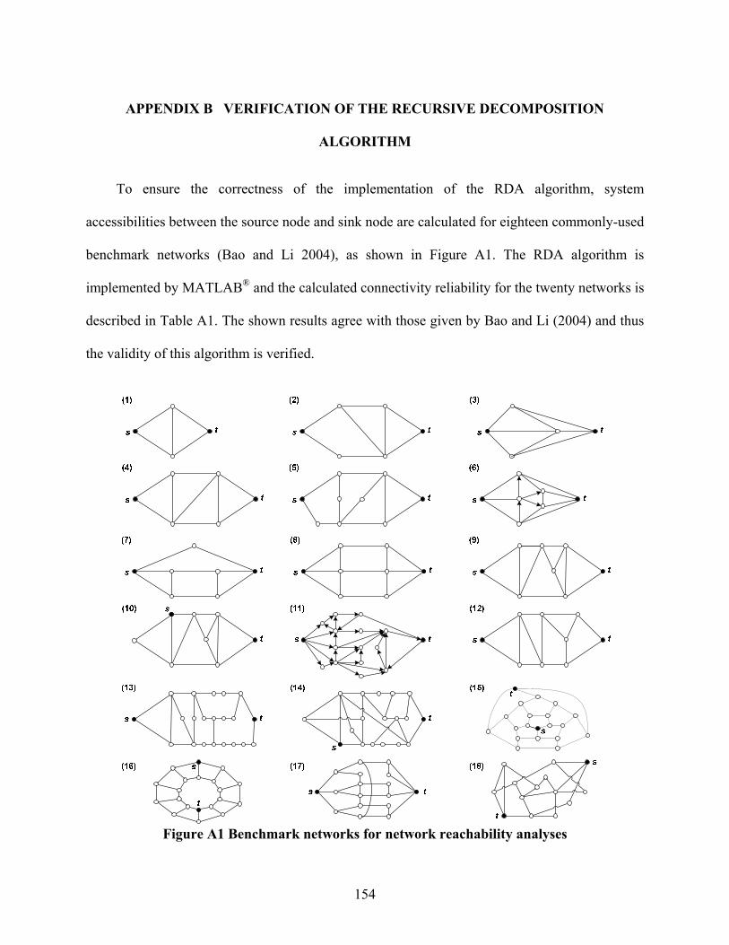
154
APPENDIX B VERIFICATION OF THE RECURSIVE DECOMPOSITION
ALGORITHM
To ensure the correctness of the implementation of the RDA algorithm, system
accessibilities between the source node and sink node are calculated for eighteen commonly-used
benchmark networks (Bao and Li 2004), as shown in Figure A1. The RDA algorithm is
implemented by MATLAB® and the calculated connectivity reliability for the twenty networks is
described in Table A1. The shown results agree with those given by Bao and Li (2004) and thus
the validity of this algorithm is verified.
Figure A1 Benchmark networks for network reachability analyses
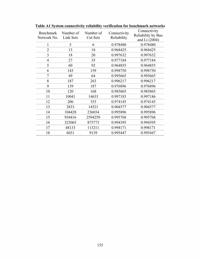
155
Table A1 System connectivity reliability verification for benchmark networks
Benchmark Network No.
Number of Link Sets
Number of Cut Sets
Connectivity Reliability
Connectivity Reliability by Bao
and Li (2004) 1 5 6 0.978480 0.978480 2 13 18 0.968425 0.968425 3 18 20 0.997632 0.997632 4 27 35 0.977184 0.977184 5 60 92 0.964855 0.964855 6 143 159 0.998750 0.998750 7 49 64 0.995665 0.995665 8 187 263 0.996217 0.996217 9 139 187 0.976896 0.976896 10 120 168 0.985865 0.985865 11 10041 14633 0.997183 0.997186 12 206 353 0.974145 0.974145 13 2833 14521 0.904577 0.904577 14 104428 236034 0.995896 0.995896 15 934416 2594259 0.995768 0.995768 16 323065 875773 0.994395 0.994395 17 48133 113211 0.998171 0.998171 18 6031 9139 0.995447 0.995447
156
APPENDIX C MODELING UNCERTAINTY AND CORRELATION OF GROUND
MOTION
This appendix discusses the uncertainty and correlation of ground motions. Relevant
literature is reviewed briefly in Section C.1. The detailed procedures for modeling the
uncertainties and correlated ground motions are presented in Section C.2. Numerical examples
are given in Section C.3 to illustrate the ground motions that incorporate the uncertainties and
spatial correlation. The generated ground motions are used in Sections 4.1 and 4.2 to study the
effects of uncertainty and correlation of ground motion on the performance of transportation
systems.
C.1 Simulation of Spatially Variable Ground Motions
Spatially variable ground motions can be simulated either with random fields through a
power spectral density and a spatial variability model, or from a predefined seismic ground
motion time history and a spatial variability model (Zerva 2008). The former approach is often
referred to as “simulation” of spatial variable seismic ground motion, while the latter is referred
to as “conditional simulation” of spatial variable seismic ground motion since it uses predefined
time histories. Although the ground motions generated with “simulation” methods bear limited
association with actual seismic records, they provide a most valuable tool for assessing the
response of spatially distributed infrastructure systems (Zerva 2008). Extensive research has
addressed the topics of generation of spatially variable ground motions with various simulation
approaches such as spectral representation, covariance matrix decomposition, conditional
simulation and interpolation. A detailed review of simulation of seismic ground motions can be
found in Zerva and Zervas (2002) and Zerva (2008).

157
C.2 Procedures
Seismic ground motions are estimated with empirical attenuation models that are defined as
a function of magnitude, distance, site classification, and fault rupture mechanism, etc. based on
stochastic simulation and regression analysis (Campbell 1985; Boore 2003; Bommer and
Crowley 2006). The general form of ground motion prediction equations can be written in the
logarithmic form as (Campbell 1985):
1 1 2 3 4ln ln ln ( ) ln ( ) ln ( , ) ln ( )iY b f M f R f M R f P (C.1)
where Y is the estimated ground motion intensity measure such as peak ground acceleration
(PGA) or the spectral response at a particular period; 1b is a scaling constant; 1( )f M is a function
of the magnitude scale M (independent variable); 2 ( )f R is a function of the measure of distance
from source to site R ( independent variable); 3 ( , )f M R is a joint function of M and R , 4 ( )if P
is a function representing parameters of earthquake, path, source, or structure; is a random
variable representing the aleatory uncertainty of Y , which results from the inherent randomness
in observed motion with respect to the predictive model (Bommer and Crowley 2006).
Following the random effects model by Abrahamson and Youngs (1992), the aleatory
uncertainty of predicted ground motion with empirical attenuation equations, can be
distinguished by inter-event uncertainty 1 and site-to-site intra-event uncertainty 2 . The inter-
event uncertainty represents the event-event variation resulting from one earthquake to another
with the same magnitude and rupture mechanism (Bommer and Crowley 2006), that is, the
“between-group” variability differences from different earthquakes. While the “within-group”
intra-event uncertainty stems from one location to another at the same distance and with the
same site classification during one earthquake (Bommer and Crowley 2006). In other words, the
variability resulting from differences in the data recorded among the different sites for the same

158
earthquake (Zhou 2006). The intra-event uncertainty is usually considered as the residual term
for spatial correlation because: (i) they have been generated by the same earthquake, (ii) the
seismic waves travel over similar path from the source to the closely-spaced sites; and (iii)
adjacent location may be located close (or far) from the asperities on the fault rupture (Park et al.
2007; Harichandran 1999).
The inter-event uncertainties and intra-event uncertainties are assumed to be independent
and normal distributed with zero means and standard deviations of and , respectively. The
basic functional form of ground motion prediction equations can thus be written as:
0 0 1 2ln ln lnY Y Y (C.2)
where 0lnY is the median value of the log of predicted ground motion (the first five terms in
Equation C.1). The standard deviation of the aleatory uncertainty is then 2 2 .
In order to accurately evaluate the impact of a scenario earthquake on the spatially
distributed infrastructure systems, both inter- and intra-event uncertainties should be estimated
when generating artificial spatial variable seismic ground motions. Because 1 is spatially
independent (Zhou 2006), it can be modeled with a normal random variable with zero mean and
the standard deviations of . However, 2 is spatially correlated with a given realization of 1 .
Random field theories have been used to generate the simulated spatial distribution of intra-event
uncertainty (Shinozuka and Jan 1972; Shinozuka et al. 1990; Shinozuka and Deodatis 1991 and
1996; Shinozuka 1971).
Spectral representation is one of the widely used approaches to simulate multi-dimensional
Gaussian random fields (Grigoriu 1993; Shinozuka and Deodatis 1996). It was first introduced
by Rice (1944) and later extended by Shinozuka (1971 and 1972). To simulate the spatial
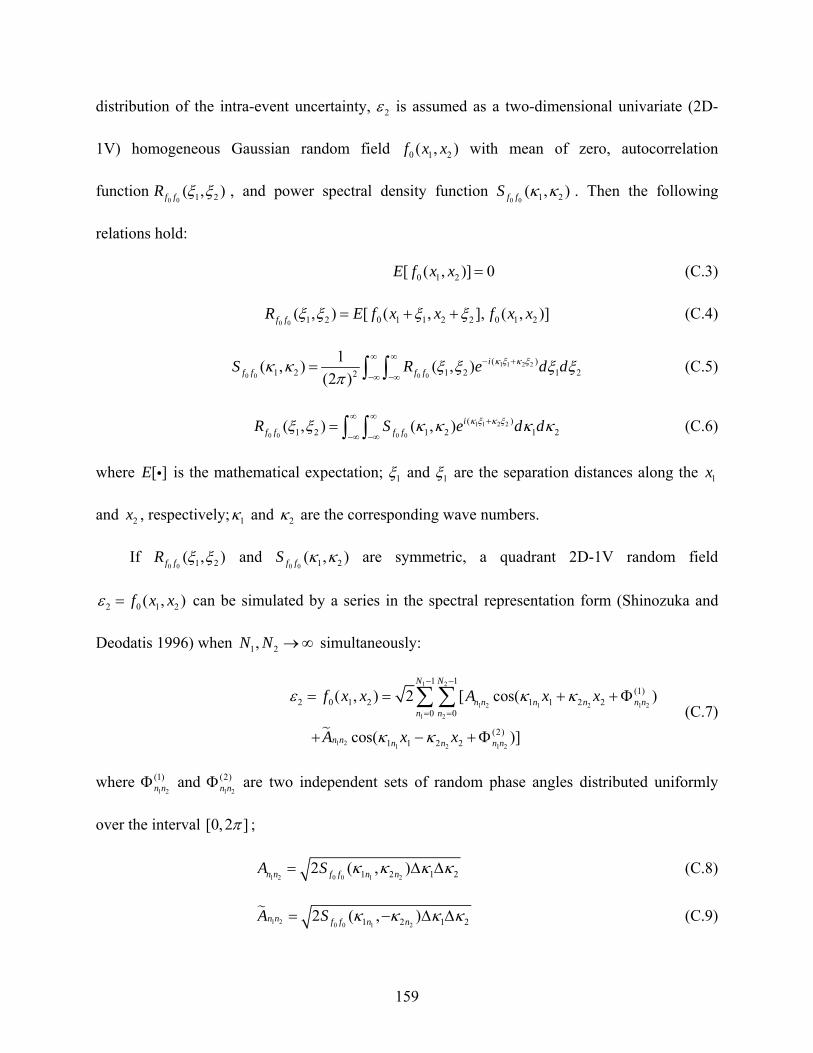
159
distribution of the intra-event uncertainty, 2 is assumed as a two-dimensional univariate (2D-
1V) homogeneous Gaussian random field 0 1 2( , )f x x with mean of zero, autocorrelation
function0 0 1 2( , )f fR , and power spectral density function
0 0 1 2( , )f fS . Then the following
relations hold:
0 1 2[ ( , )] 0E f x x (C.3)
0 0 1 2 0 1 1 2 2 0 1 2( , ) [ ( , ], ( , )]f fR E f x x f x x (C.4)
1 1 2 2
0 0 0 0
( )1 2 1 2 1 22
1( , ) ( , )
(2 )i
f f f fS R e d d
(C.5)
1 1 2 2
0 0 0 0
( )1 2 1 2 1 2( , ) ( , ) i
f f f fR S e d d
(C.6)
where [ ]E is the mathematical expectation; 1 and 1 are the separation distances along the 1x
and 2x , respectively; 1 and 2 are the corresponding wave numbers.
If 0 0 1 2( , )f fR and
0 0 1 2( , )f fS are symmetric, a quadrant 2D-1V random field
2 0 1 2( , )f x x can be simulated by a series in the spectral representation form (Shinozuka and
Deodatis 1996) when 1 2,N N simultaneously:
1 2
1 2 1 2 1 2
1 2
1 2 1 2 1 2
1 1(1)
2 0 1 2 1 1 2 20 0
(2)1 1 2 2
( , ) 2 [ cos( )
cos( )]
N N
n n n n n nn n
n n n n n n
f x x A x x
A x x
(C.7)
where 1 2
(1)n n and
1 2
(2)n n are two independent sets of random phase angles distributed uniformly
over the interval [0,2 ] ;
1 2 0 0 1 21 2 1 22 ( , )n n f f n nA S (C.8)
1 2 0 0 1 21 2 1 22 ( , )n n f f n nA S (C.9)
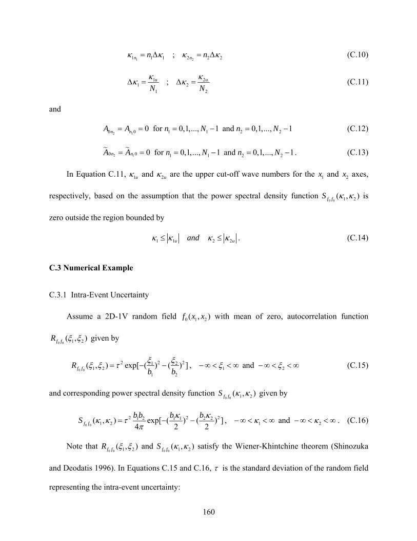
160
1 21 1 1 2 2 2;n nn n (C.10)
1 21 2
1 2
;u u
N N
(C.11)
and
2 10 0 1 1 2 20 for 0,1,..., 1 and 0,1,..., 1n nA A n N n N (C.12)
2 10 0 1 1 2 20 for 0,1,..., 1 and 0,1,..., 1n nA A n N n N . (C.13)
In Equation C.11, 1u and 2u are the upper cut-off wave numbers for the 1x and 2x axes,
respectively, based on the assumption that the power spectral density function 0 0 1 2( , )f fS is
zero outside the region bounded by
1 1 2 2u uand . (C.14)
C.3 Numerical Example
C.3.1 Intra-Event Uncertainty
Assume a 2D-1V random field 0 1 2( , )f x x with mean of zero, autocorrelation function
0 0 1 2( , )f fR given by
0 0
2 2 21 21 2 1 2
1 2
( , ) exp[ ( ) ( ) ] , andf fRb b
(C.15)
and corresponding power spectral density function 0 0 1 2( , )f fS given by
0 0
2 2 21 2 1 1 2 21 2 1 2( , ) exp[ ( ) ( ) ] , and
4 2 2f f
b b b bS
. (C.16)
Note that 0 0 1 2( , )f fR and
0 0 1 2( , )f fS satisfy the Wiener-Khintchine theorem (Shinozuka
and Deodatis 1996). In Equations C.15 and C.16, is the standard deviation of the random field
representing the intra-event uncertainty:
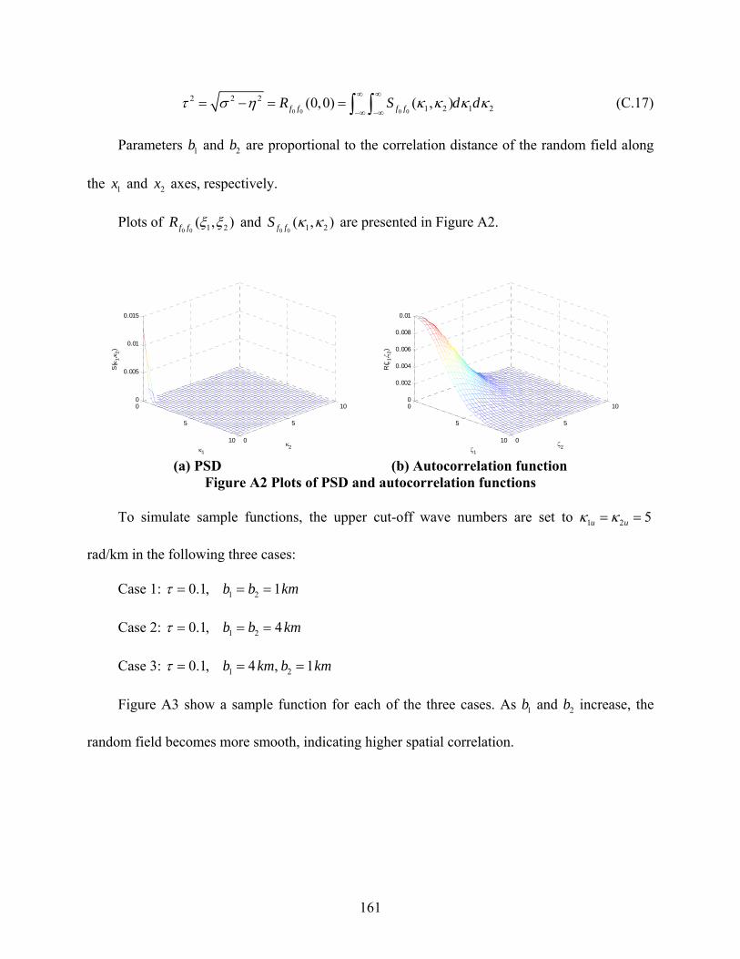
161
0 0 0 0
2 2 21 2 1 2(0,0) ( , )f f f fR S d d
(C.17)
Parameters 1b and 2b are proportional to the correlation distance of the random field along
the 1x and 2x axes, respectively.
Plots of 0 0 1 2( , )f fR and
0 0 1 2( , )f fS are presented in Figure A2.
(a) PSD (b) Autocorrelation function
Figure A2 Plots of PSD and autocorrelation functions
To simulate sample functions, the upper cut-off wave numbers are set to 1 2 5u u
rad/km in the following three cases:
Case 1: 1 20.1, 1b b km
Case 2: 1 20.1, 4b b km
Case 3: 1 20.1, 4 , 1b km b km
Figure A3 show a sample function for each of the three cases. As 1b and 2b increase, the
random field becomes more smooth, indicating higher spatial correlation.
0
5
10 0
5
100
0.002
0.004
0.006
0.008
0.01
21
R(
1, 2
)
0
5
10 0
5
100
0.005
0.01
0.015
21
S(
1, 2
)
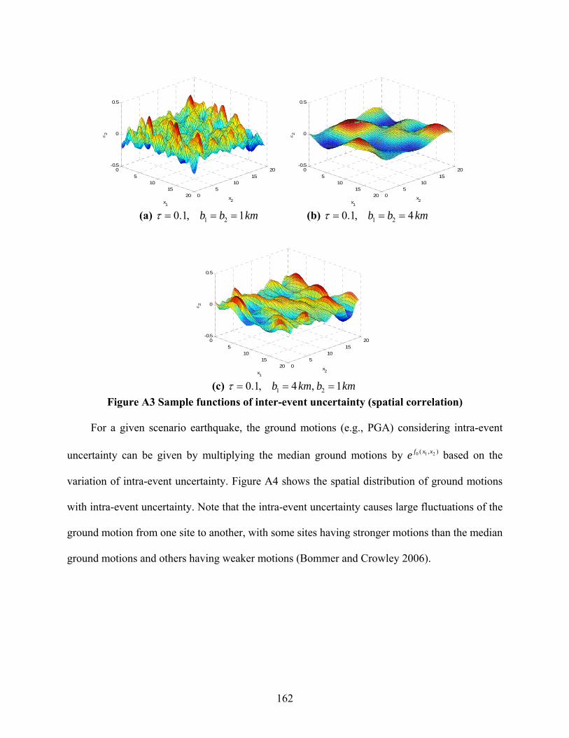
162
0
510
1520 0
510
15
20-0.5
0
0.5
x2x
1
2
0
510
1520 0
510
15
20-0.5
0
0.5
x2x
1
2
(a) 1 20.1, 1b b km (b) 1 20.1, 4b b km
0
510
1520 0
510
15
20-0.5
0
0.5
x2x
1
2
(c) 1 20.1, 4 , 1b km b km
Figure A3 Sample functions of inter-event uncertainty (spatial correlation)
For a given scenario earthquake, the ground motions (e.g., PGA) considering intra-event
uncertainty can be given by multiplying the median ground motions by 0 1 2( , )f x xe based on the
variation of intra-event uncertainty. Figure A4 shows the spatial distribution of ground motions
with intra-event uncertainty. Note that the intra-event uncertainty causes large fluctuations of the
ground motion from one site to another, with some sites having stronger motions than the median
ground motions and others having weaker motions (Bommer and Crowley 2006).
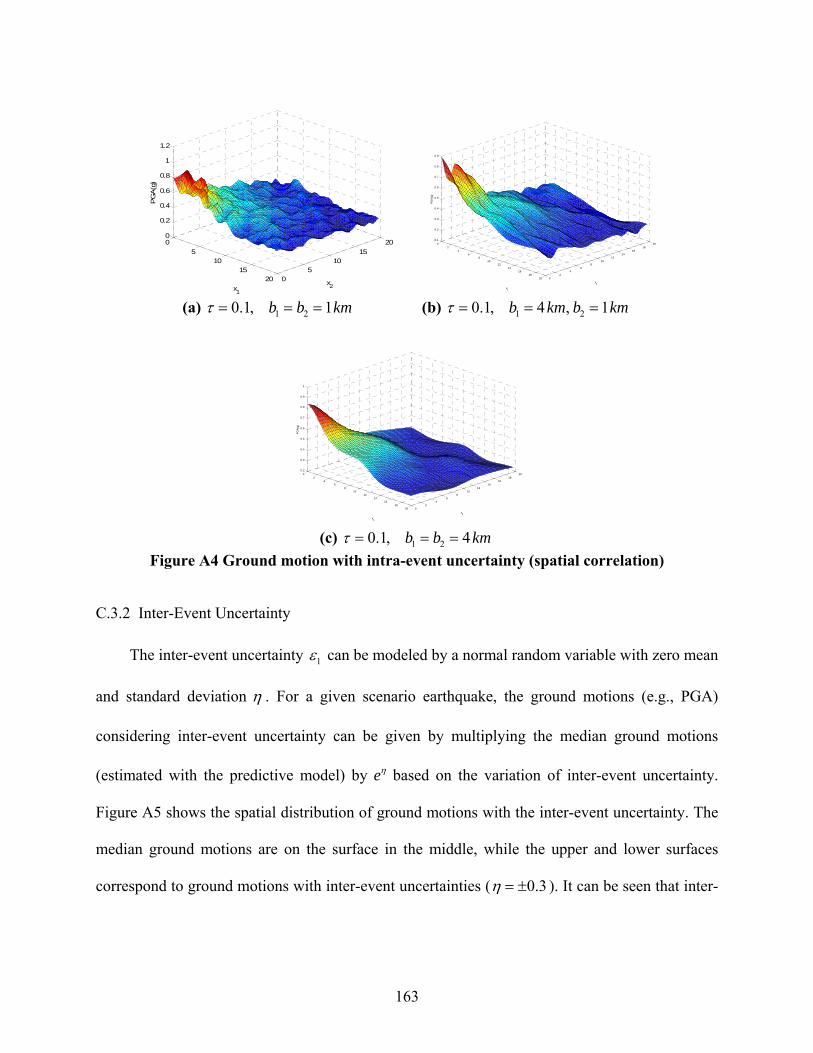
163
0
510
1520 0
510
15
200
0.2
0.4
0.6
0.8
1
1.2
x2x
1
PG
A(g
)
02
46
810
1214
1618
20 02
46
810
1214
1618
200.1
0.2
0.3
0.4
0.5
0.6
0.7
0.8
0.9
x2
x1
PG
A(g
)
(a) 1 20.1, 1b b km (b) 1 20.1, 4 , 1b km b km
02
46
810
1214
1618
20 02
46
810
1214
1618
200.2
0.3
0.4
0.5
0.6
0.7
0.8
0.9
1
x2
x1
PG
A(g
)
(c) 1 20.1, 4b b km
Figure A4 Ground motion with intra-event uncertainty (spatial correlation)
C.3.2 Inter-Event Uncertainty
The inter-event uncertainty 1 can be modeled by a normal random variable with zero mean
and standard deviation . For a given scenario earthquake, the ground motions (e.g., PGA)
considering inter-event uncertainty can be given by multiplying the median ground motions
(estimated with the predictive model) by e based on the variation of inter-event uncertainty.
Figure A5 shows the spatial distribution of ground motions with the inter-event uncertainty. The
median ground motions are on the surface in the middle, while the upper and lower surfaces
correspond to ground motions with inter-event uncertainties ( 0.3 ). It can be seen that inter-

164
event uncertainty leads to the ground motions at all locations to be smaller or larger than the
median PGA from the predictive model.
0
510
1520 0
510
15
200
0.5
1
1.5
Figure A5 Sample function of intra-event uncertainty
C.3.3 Consideration of both Inter- and Intra-Event Uncertainties
When considering both inter- and intra-event uncertainties, the ground motions can be
obtained by multiplying the spatial distribution of median ground motions by 0 1 2( , )f x xe based on
the variation of intra- and inter-event uncertainties. As shown in Figure A6, the fluctuation of
spatial distribution of ground motions will cause different motions under the same scenario
earthquake. By combining these two uncertainties with the median ground motions from
scenario earthquakes, it is possible to investigate their effects on the seismic performance of
spatially distributed infrastructure systems such as transportation networks.
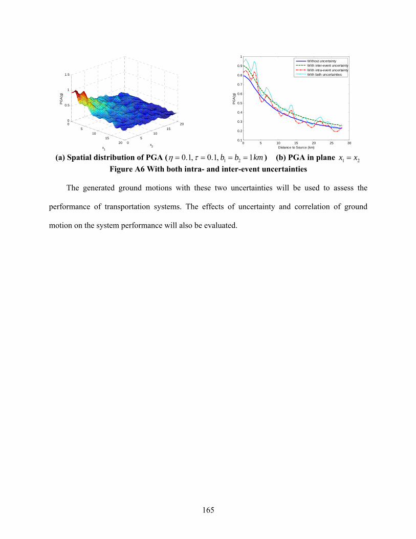
165
0
510
1520 0
510
15
200
0.5
1
1.5
x2x
1
PG
A(g
)
0 5 10 15 20 25 30
0.1
0.2
0.3
0.4
0.5
0.6
0.7
0.8
0.9
1
Distance to Source (km)
PG
A(g
)
Without uncertaintyWith inter-event uncertaintyWith intra-event uncertaintyWith both uncertainties
(a) Spatial distribution of PGA ( 1 20.1, 0.1, 1b b km ) (b) PGA in plane 1 2x x
Figure A6 With both intra- and inter-event uncertainties
The generated ground motions with these two uncertainties will be used to assess the
performance of transportation systems. The effects of uncertainty and correlation of ground
motion on the system performance will also be evaluated.
166
APPENDIX D VERIFICATION OF THE DUE MODELS
In order to verify the traffic modeling results given by the DUE model, an approximate
method is employed to estimate the lower and upper bounds of the total system travel time. The
underlying idea of this approach is to use the shortest path (based on free-flow conditions) at
unloaded and loaded states to give an estimation of the simulated travel time (Waller 2008). The
procedures of this method are detailed below for the given transportation networks and
corresponding travel demand.
For every OD pair in the travel demand data, first the corresponding shortest path ( SP )
between the origin and destination is identified. The lower bound of the total travel cost, LB
TSTT
can be calculated with the following formula since each OD pair is getting its free-flow travel
time:
( , ) ( , )LB
i j
TSTT d i j G i j (D.1)
where ( , )SP i j denotes the shortest path between nodes i and j , ( , )G i j is the free flow cost of
( , )SP i j , and ( , )d i j is the travel demand nodes i and j .
The upper bound of the total travel cost can be found with similar idea. By adding the travel
flow ( , )d i j to every link along the shortest path ( , )SP i j , a new travel cost ( , )H i j can be
calculated, which is the cost of the path between nodes i and j with all the trips assigned to
their shortest paths. By summing up the travel costs for all the OD pairs, the upper bound on the
total travel cost, UB
TSTT can be written as
( , ) ( , )UBi j
TSTT d i j H i j (D.2)
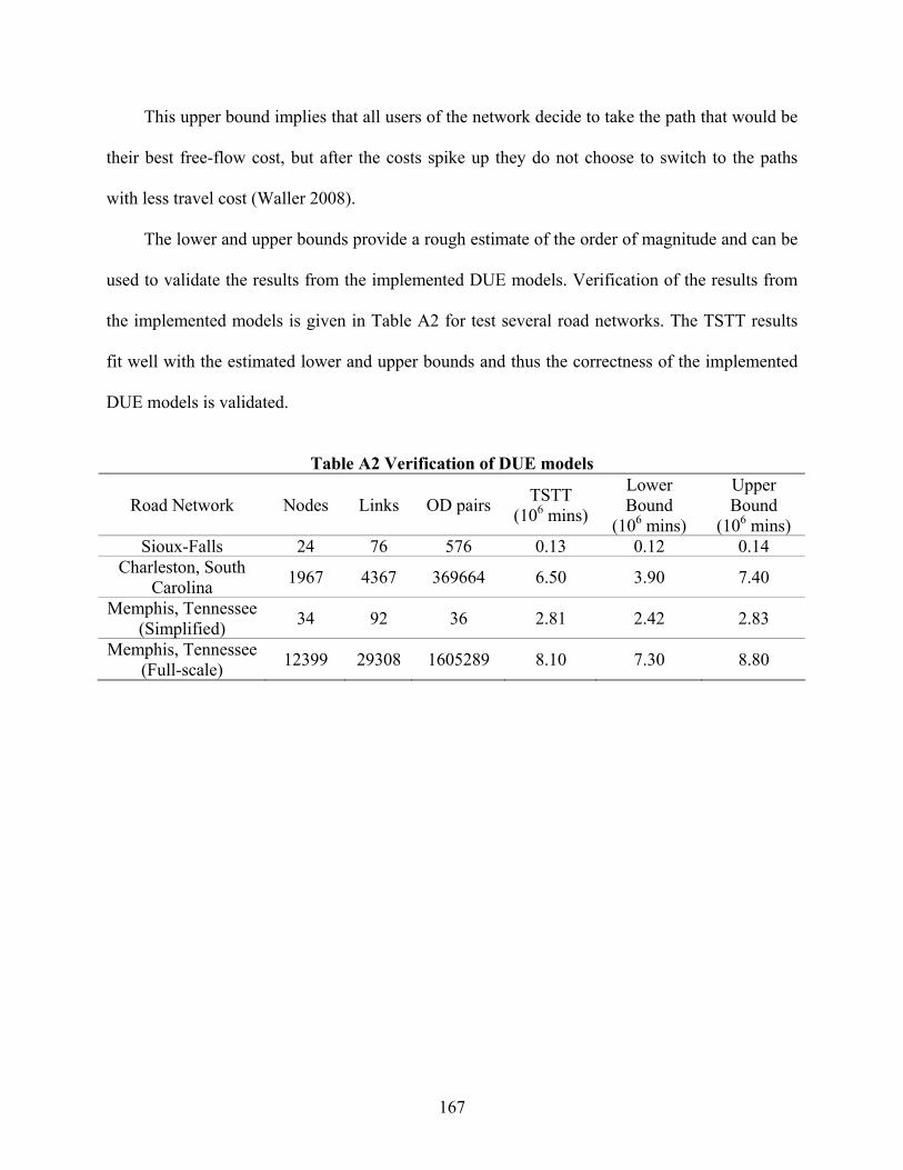
167
This upper bound implies that all users of the network decide to take the path that would be
their best free-flow cost, but after the costs spike up they do not choose to switch to the paths
with less travel cost (Waller 2008).
The lower and upper bounds provide a rough estimate of the order of magnitude and can be
used to validate the results from the implemented DUE models. Verification of the results from
the implemented models is given in Table A2 for test several road networks. The TSTT results
fit well with the estimated lower and upper bounds and thus the correctness of the implemented
DUE models is validated.
Table A2 Verification of DUE models
Road Network Nodes Links OD pairs TSTT
(106 mins)
Lower Bound
(106 mins)
Upper Bound
(106 mins) Sioux-Falls 24 76 576 0.13 0.12 0.14
Charleston, South Carolina
1967 4367 369664 6.50 3.90 7.40
Memphis, Tennessee (Simplified)
34 92 36 2.81 2.42 2.83
Memphis, Tennessee (Full-scale)
12399 29308 1605289 8.10 7.30 8.80
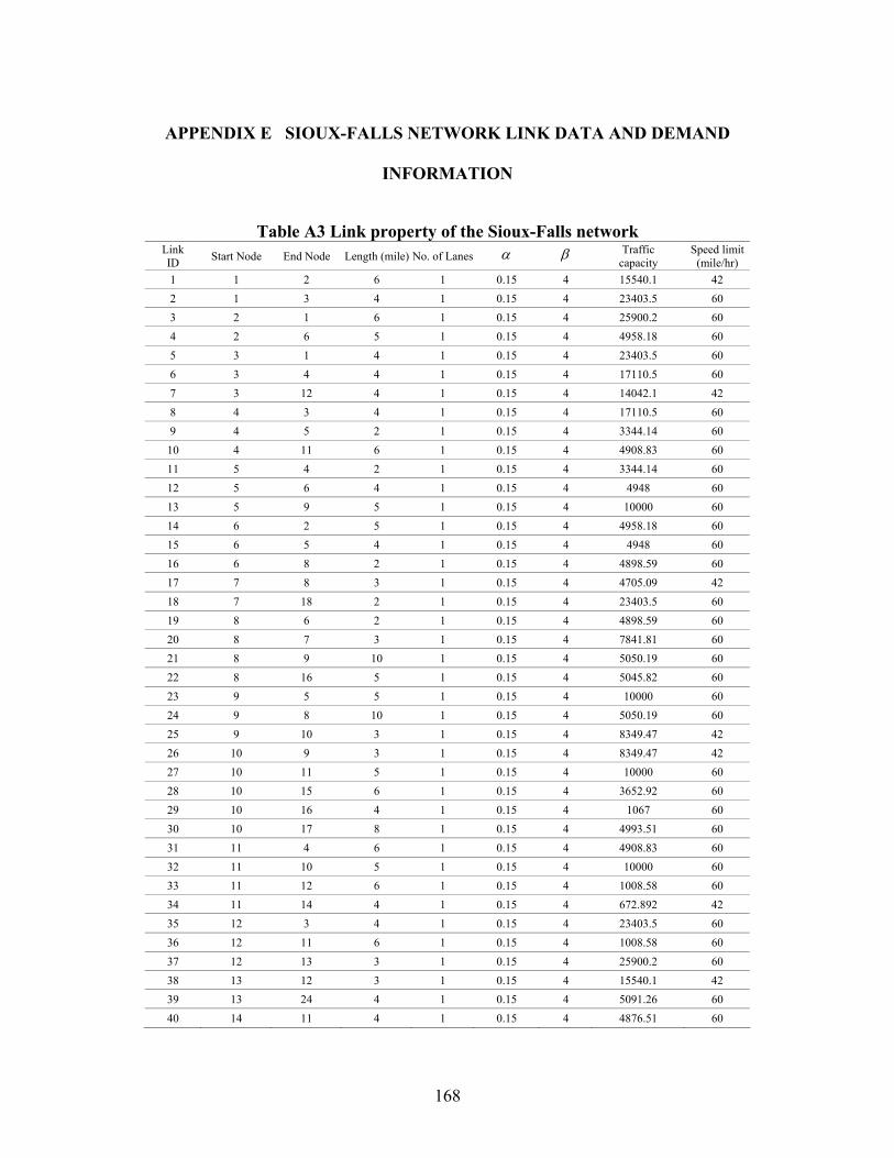
168
APPENDIX E SIOUX-FALLS NETWORK LINK DATA AND DEMAND
INFORMATION
Table A3 Link property of the Sioux-Falls network Link ID
Start Node End Node Length (mile) No. of Lanes Traffic capacity
Speed limit (mile/hr)
1 1 2 6 1 0.15 4 15540.1 42
2 1 3 4 1 0.15 4 23403.5 60
3 2 1 6 1 0.15 4 25900.2 60
4 2 6 5 1 0.15 4 4958.18 60
5 3 1 4 1 0.15 4 23403.5 60
6 3 4 4 1 0.15 4 17110.5 60
7 3 12 4 1 0.15 4 14042.1 42
8 4 3 4 1 0.15 4 17110.5 60
9 4 5 2 1 0.15 4 3344.14 60
10 4 11 6 1 0.15 4 4908.83 60
11 5 4 2 1 0.15 4 3344.14 60
12 5 6 4 1 0.15 4 4948 60
13 5 9 5 1 0.15 4 10000 60
14 6 2 5 1 0.15 4 4958.18 60
15 6 5 4 1 0.15 4 4948 60
16 6 8 2 1 0.15 4 4898.59 60
17 7 8 3 1 0.15 4 4705.09 42
18 7 18 2 1 0.15 4 23403.5 60
19 8 6 2 1 0.15 4 4898.59 60
20 8 7 3 1 0.15 4 7841.81 60
21 8 9 10 1 0.15 4 5050.19 60
22 8 16 5 1 0.15 4 5045.82 60
23 9 5 5 1 0.15 4 10000 60
24 9 8 10 1 0.15 4 5050.19 60
25 9 10 3 1 0.15 4 8349.47 42
26 10 9 3 1 0.15 4 8349.47 42
27 10 11 5 1 0.15 4 10000 60
28 10 15 6 1 0.15 4 3652.92 60
29 10 16 4 1 0.15 4 1067 60
30 10 17 8 1 0.15 4 4993.51 60
31 11 4 6 1 0.15 4 4908.83 60
32 11 10 5 1 0.15 4 10000 60
33 11 12 6 1 0.15 4 1008.58 60
34 11 14 4 1 0.15 4 672.892 42
35 12 3 4 1 0.15 4 23403.5 60
36 12 11 6 1 0.15 4 1008.58 60
37 12 13 3 1 0.15 4 25900.2 60
38 13 12 3 1 0.15 4 15540.1 42
39 13 24 4 1 0.15 4 5091.26 60
40 14 11 4 1 0.15 4 4876.51 60
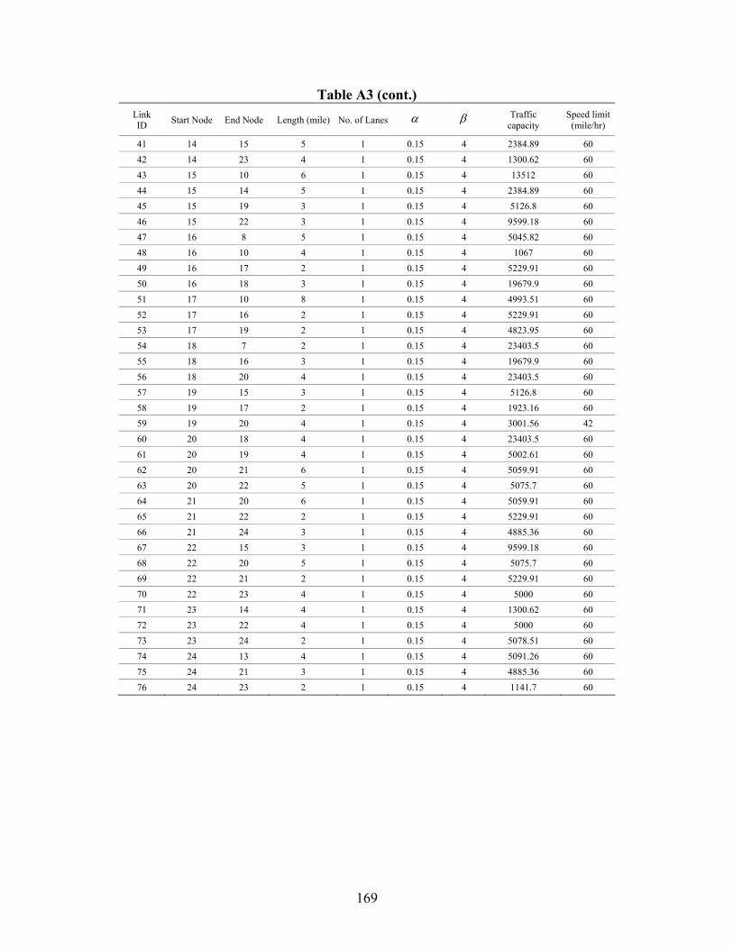
169
Table A3 (cont.) Link ID
Start Node End Node Length (mile) No. of Lanes Traffic capacity
Speed limit (mile/hr)
41 14 15 5 1 0.15 4 2384.89 60
42 14 23 4 1 0.15 4 1300.62 60
43 15 10 6 1 0.15 4 13512 60
44 15 14 5 1 0.15 4 2384.89 60
45 15 19 3 1 0.15 4 5126.8 60
46 15 22 3 1 0.15 4 9599.18 60
47 16 8 5 1 0.15 4 5045.82 60
48 16 10 4 1 0.15 4 1067 60
49 16 17 2 1 0.15 4 5229.91 60
50 16 18 3 1 0.15 4 19679.9 60
51 17 10 8 1 0.15 4 4993.51 60
52 17 16 2 1 0.15 4 5229.91 60
53 17 19 2 1 0.15 4 4823.95 60
54 18 7 2 1 0.15 4 23403.5 60
55 18 16 3 1 0.15 4 19679.9 60
56 18 20 4 1 0.15 4 23403.5 60
57 19 15 3 1 0.15 4 5126.8 60
58 19 17 2 1 0.15 4 1923.16 60
59 19 20 4 1 0.15 4 3001.56 42
60 20 18 4 1 0.15 4 23403.5 60
61 20 19 4 1 0.15 4 5002.61 60
62 20 21 6 1 0.15 4 5059.91 60
63 20 22 5 1 0.15 4 5075.7 60
64 21 20 6 1 0.15 4 5059.91 60
65 21 22 2 1 0.15 4 5229.91 60
66 21 24 3 1 0.15 4 4885.36 60
67 22 15 3 1 0.15 4 9599.18 60
68 22 20 5 1 0.15 4 5075.7 60
69 22 21 2 1 0.15 4 5229.91 60
70 22 23 4 1 0.15 4 5000 60
71 23 14 4 1 0.15 4 1300.62 60
72 23 22 4 1 0.15 4 5000 60
73 23 24 2 1 0.15 4 5078.51 60
74 24 13 4 1 0.15 4 5091.26 60
75 24 21 3 1 0.15 4 4885.36 60
76 24 23 2 1 0.15 4 1141.7 60

170
Table A4 Origin-destination matrix for Sioux-Falls network (night scenario) Destination
Origin 1 2 3 4 5 6 7 8 9 10 11 12 13 14 15 16 17 18 19 20 21 22 23 24
1 2 12 6 30 6 14 30 54 20 84 20 6 38 14 30 30 22 6 22 14 2 22 14 2
2 24 2 24 24 16 40 24 40 14 46 14 16 40 16 16 40 24 16 24 16 8 16 8 8
3 6 12 2 6 2 14 2 6 12 4 4 6 6 2 2 6 2 2 2 10 10 2 2 10
4 48 6 24 0 40 32 32 56 46 86 102 48 56 40 40 64 40 16 24 24 16 32 40 16
5 24 2 16 40 0 16 16 40 54 70 30 16 24 8 16 40 16 8 16 8 8 16 8 0
6 32 22 32 32 16 0 32 64 22 54 22 16 24 8 16 72 40 16 24 24 8 16 8 8
7 48 6 16 32 16 32 0 80 38 142 30 56 40 16 40 112 80 24 40 40 16 40 16 8
8 72 22 24 56 40 64 80 0 54 118 54 48 56 32 48 176 112 32 64 72 32 40 24 16
9 56 14 24 64 72 40 56 72 2 222 110 56 64 56 80 120 80 32 48 56 32 64 48 24
10 120 46 40 104 88 72 160 136 222 2 318 168 168 176 328 360 320 72 160 208 104 216 152 72
11 56 14 40 128 48 40 48 72 110 310 2 120 96 136 120 120 88 24 48 56 40 96 112 56
12 24 2 24 48 16 16 56 48 38 150 102 0 112 56 56 56 48 24 32 32 24 56 56 40
13 38 4 6 38 6 6 22 38 28 132 60 94 2 38 46 38 30 6 22 38 38 94 54 54
14 32 2 16 40 8 8 16 32 38 158 118 56 56 0 104 56 56 16 32 40 32 96 88 32
15 48 2 16 40 16 16 40 48 70 310 102 56 64 104 0 96 120 24 72 88 64 208 80 32
16 48 22 24 64 40 72 112 176 102 342 102 56 56 56 96 0 224 48 112 128 48 96 40 24
17 40 6 16 40 16 40 80 112 62 302 70 48 48 56 120 224 0 56 144 136 48 136 48 24
18 6 20 2 2 10 2 6 14 4 36 4 6 6 2 6 30 38 2 22 22 2 14 2 10
19 22 12 2 6 2 6 22 46 12 124 12 14 22 14 54 94 126 22 2 86 22 86 14 2
20 32 2 8 24 8 24 40 72 38 190 38 40 56 40 88 128 136 40 104 0 96 192 56 32
21 16 10 8 16 8 8 16 32 14 86 22 24 56 32 64 48 48 16 40 96 0 144 56 40
22 40 2 16 32 16 16 40 40 46 198 78 56 112 96 208 96 136 32 104 192 144 0 168 88
23 32 10 16 40 8 8 16 24 30 134 94 56 72 88 80 40 48 16 32 56 56 168 0 56
24 16 10 8 16 0 8 8 16 6 54 38 40 64 32 32 24 24 8 16 32 40 88 56 0
Table A5 Origin-destination matrix for Sioux-Falls network (day scenario)
Destination
Origin 1 2 3 4 5 6 7 8 9 10 11 12 13 14 15 16 17 18 19 20 21 22 23 24
1 200 900 300 800 500 600 800 1100 1300 2100 1300 500 700 600 800 800 700 300 500 600 400 700 600 400
2 100 400 100 100 0 300 100 300 600 1000 600 0 100 0 0 300 100 200 100 0 100 0 100 100
3 300 900 200 500 400 600 400 500 900 1100 1100 500 300 400 400 500 400 200 200 300 300 400 400 300
4 400 700 100 0 500 400 400 700 1200 1700 1900 600 500 500 500 800 500 0 100 300 200 400 500 200
5 100 600 0 500 0 200 200 500 1300 1500 1000 200 100 100 200 500 200 100 0 100 100 200 100 0
6 200 900 200 400 200 0 400 800 900 1300 900 200 100 100 200 900 500 0 100 300 100 200 100 100
7 400 700 0 400 200 400 0 1000 1100 2400 1000 700 300 200 500 1400 1000 100 300 500 200 500 200 100
8 700 900 100 700 500 800 1000 0 1300 2100 1300 600 500 400 600 2200 1400 200 600 900 400 500 300 200
9 300 600 100 600 700 300 500 700 400 3200 1800 500 400 500 800 1300 800 0 200 500 200 600 400 100
10 1100 1000 100 1100 900 700 1800 1500 3200 400 4400 1900 1700 2000 3900 4300 3800 500 1600 2400 1100 2500 1700 700
11 300 600 100 1400 400 300 400 700 1800 4300 400 1300 800 1500 1300 1300 900 100 200 500 300 1000 1200 500
12 100 600 100 600 200 200 700 600 1100 2500 1900 0 1200 700 700 700 600 100 200 400 300 700 700 500
13 700 1100 300 900 500 500 700 900 1400 2700 1800 1600 200 900 1000 900 800 300 500 900 900 1600 1100 1100
14 200 600 0 500 100 100 200 400 1100 2600 2100 700 500 0 1300 700 700 0 200 500 400 1200 1100 400
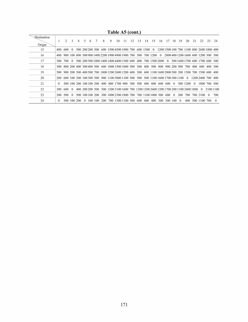
171
Table A5 (cont.) Destination
Origin
1 2 3 4 5 6 7 8 9 10 11 12 13 14 15 16 17 18 19 20 21 22 23 24
15 400 600 0 500 200 200 500 600 1500 4500 1900 700 600 1300 0 1200 1500 100 700 1100 800 2600 1000 400
16 400 900 100 800 500 900 1400 2200 1900 4900 1900 700 500 700 1200 0 2800 400 1200 1600 600 1200 500 300
17 300 700 0 500 200 500 1000 1400 1400 4400 1500 600 400 700 1500 2800 0 500 1600 1700 600 1700 600 300
18 300 800 200 400 300 400 500 600 1000 1500 1000 500 300 400 500 800 900 200 500 700 400 600 400 300
19 500 900 200 500 400 500 700 1000 1200 2600 1200 600 500 600 1100 1600 2000 500 200 1500 700 1500 600 400
20 200 600 100 300 100 300 500 900 1100 3000 1100 500 500 500 1100 1600 1700 300 1100 0 1200 2400 700 400
21 0 500 100 200 100 100 200 400 800 1700 900 300 500 400 800 600 600 0 300 1200 0 1800 700 500
22 300 600 0 400 200 200 500 500 1200 3100 1600 700 1200 1200 2600 1200 1700 200 1100 2400 1800 0 2100 1100
23 200 500 0 500 100 100 200 300 1000 2300 1800 700 700 1100 1000 500 600 0 200 700 700 2100 0 700
24 0 500 100 200 0 100 100 200 700 1300 1100 500 600 400 400 300 300 100 0 400 500 1100 700 0