Transportation Systems as Networks

Using graph analyses we are interested in measuring such things as:

1. Traffic generated by nodes.

2. Flow along links.

3. Degree of accessibility and connectivity.

4. Spatial extent of a network.

5. Network association along a route.

6. Influence of one place on other places on a route or in a network.

Graph theory – reduces transport networks to a mathematical matrix whereby: Edge: Line segment (link) between locations.

• Example: roads, rail lines, etc… Vertex: Location on the transportation network that is of interest (node).

• Example: towns, road intersections, etc… In transportation analysis graphs are ALWAYS finite… there are always constraining boundaries.

Node – a location on a transportation route that has the capacity to generate traffic (flow). Link – the connection between 2 nodes along which flow occurs. Route – a series of connected links. Network – a system of nodes and links. May consist of several modal types (road, rail, etc…), but is typically of a single mode type.

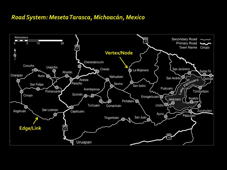
Road System: Meseta Tarasca, Michoacán, Mexico

Edge/Link

Vertex/Node

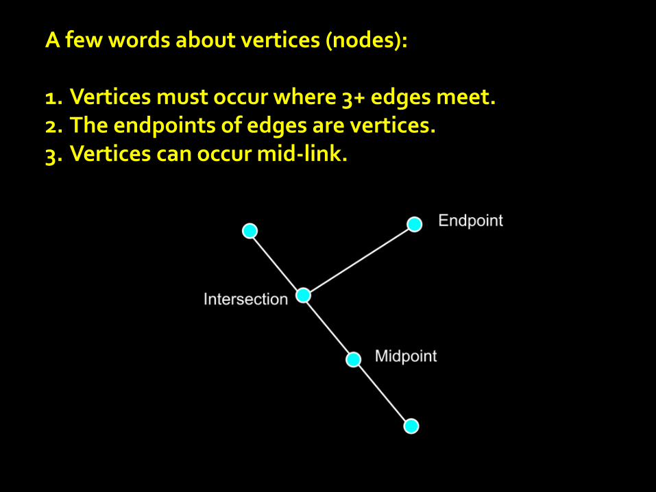
A few words about vertices (nodes): 1. Vertices must occur where 3+ edges meet. 2. The endpoints of edges are vertices. 3. Vertices can occur mid-link.

Directed graph – direction of flow is explicit. Undirected graph – no flow direction implied. Loop – flow from a node into itself. Planar – graphs where all links (edges) meet at nodes (vertices). Non-planar – graphs where links (edges) may cross each other. Element – a graph cell (dyad).

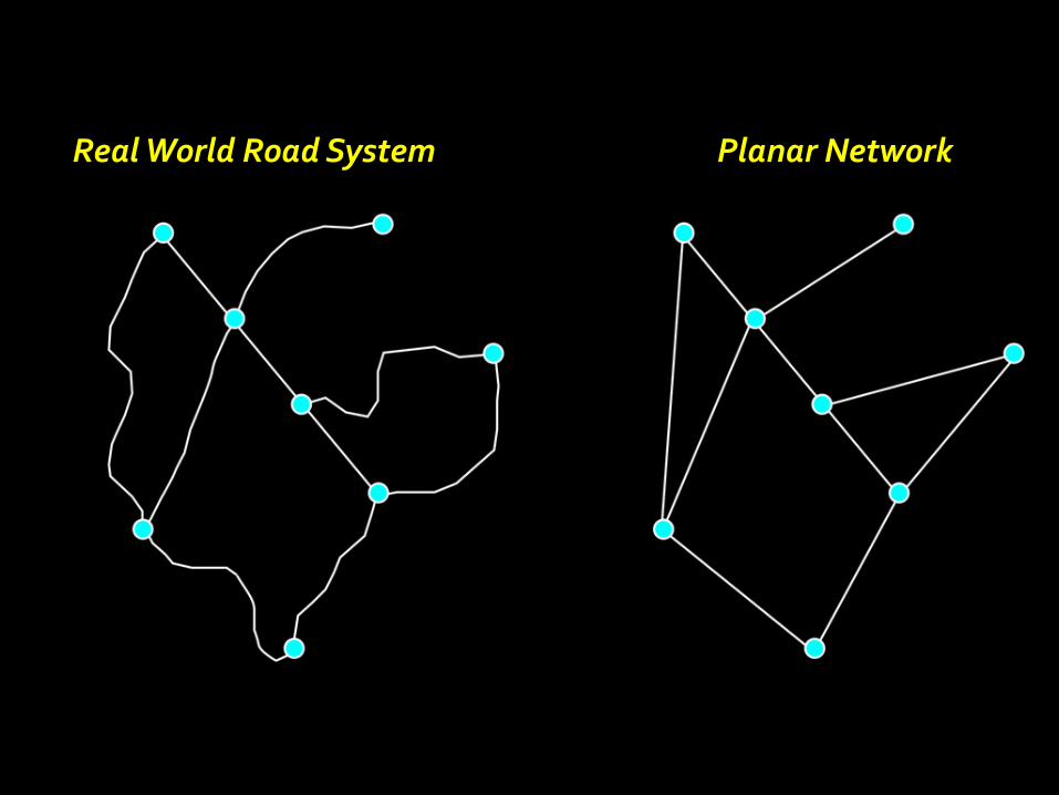
Real World Road System Planar Network

Topologic (geometric) distance – a unit-less measure where the distance between nodes is coded as a single step. • Distance is ONLY implied (e.g. more steps = longer

distance.

• Real world distances are not used. • Essentially removes the influence of distance.

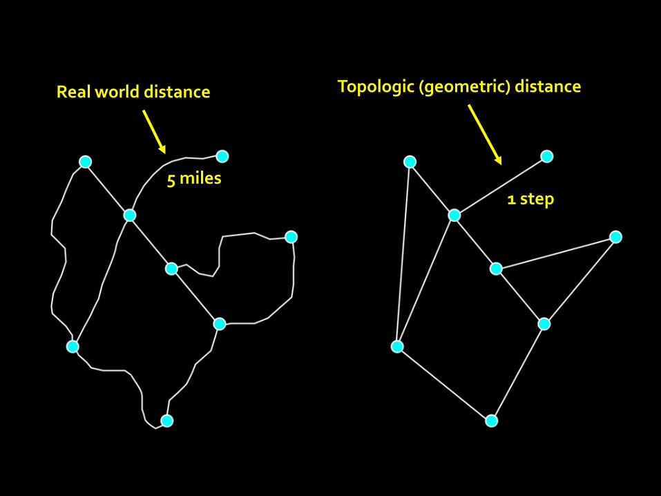
Real world distance Topologic (geometric) distance

7 miles 1 step

5 miles 1 step

Vertices = 8 Edges = 10

Example Graph

Diameter – the number of links needed to connect the two most remote nodes in a network.

• The route used must be the shortest possible.

• Backtracks, loops, and detours are excluded.

• Sometimes referred to as the ‘longest, shortest path’.

In other words, the diameter is the maximum number of steps to connect any two points on a graph.

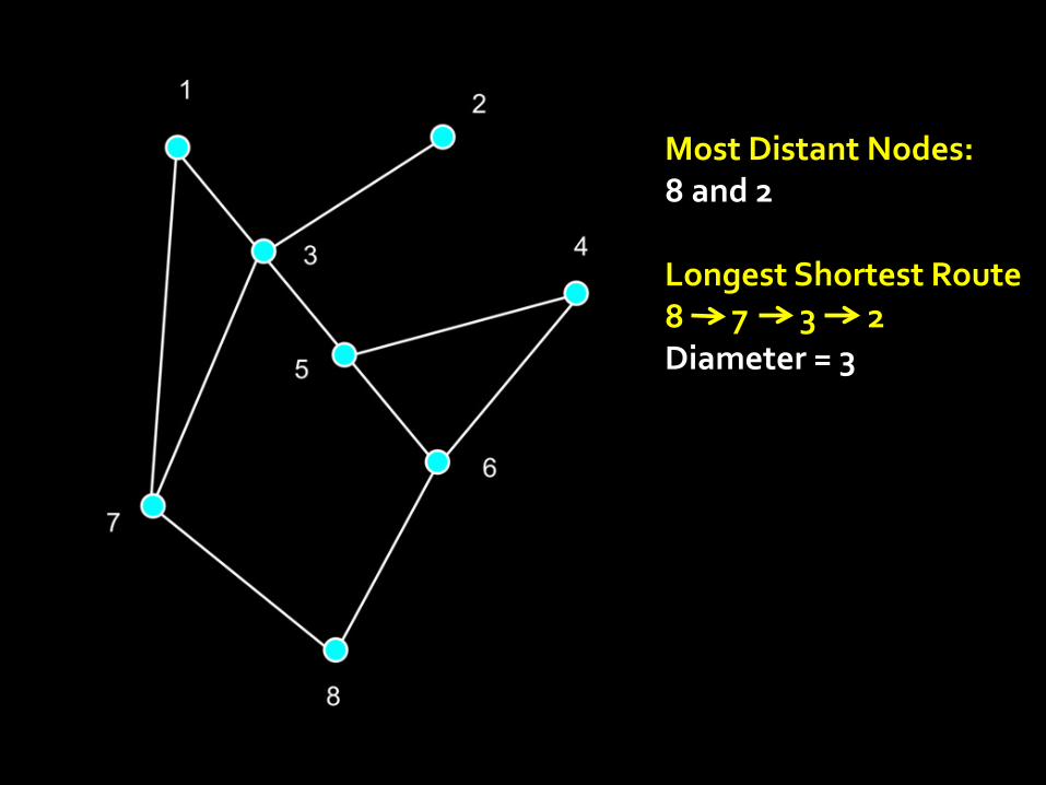
Most Distant Nodes: 8 and 2 Longest Shortest Route 8 7 3 2 Diameter = 3

Tree – a connected acyclic simple graph, which therefore has no complete circuits.

Simple graph Tree

Circuit

Circuit

Circuit

Cyclomatic Number – An index that is the difference between the number of edges and vertices. where μ is the cyclomatic number, e is the number of edges, v is the number of vertices, and p is the number of subgraphs. Note: in most cases p = 1.

μ = e – v + p

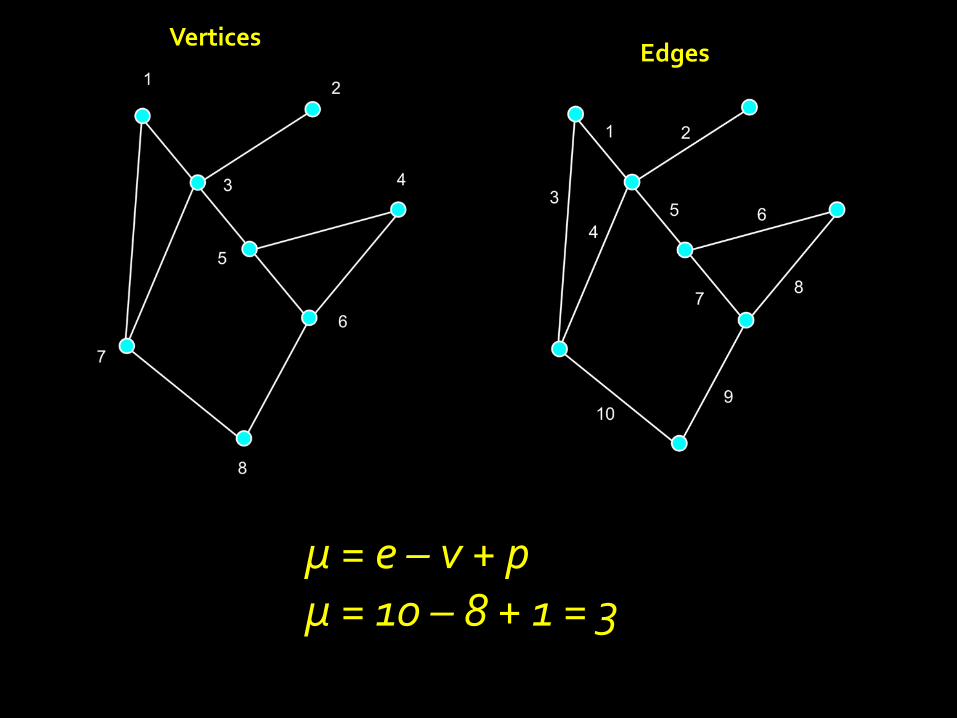
Vertices Edges

μ = e – v + p μ = 10 – 8 + 1 = 3

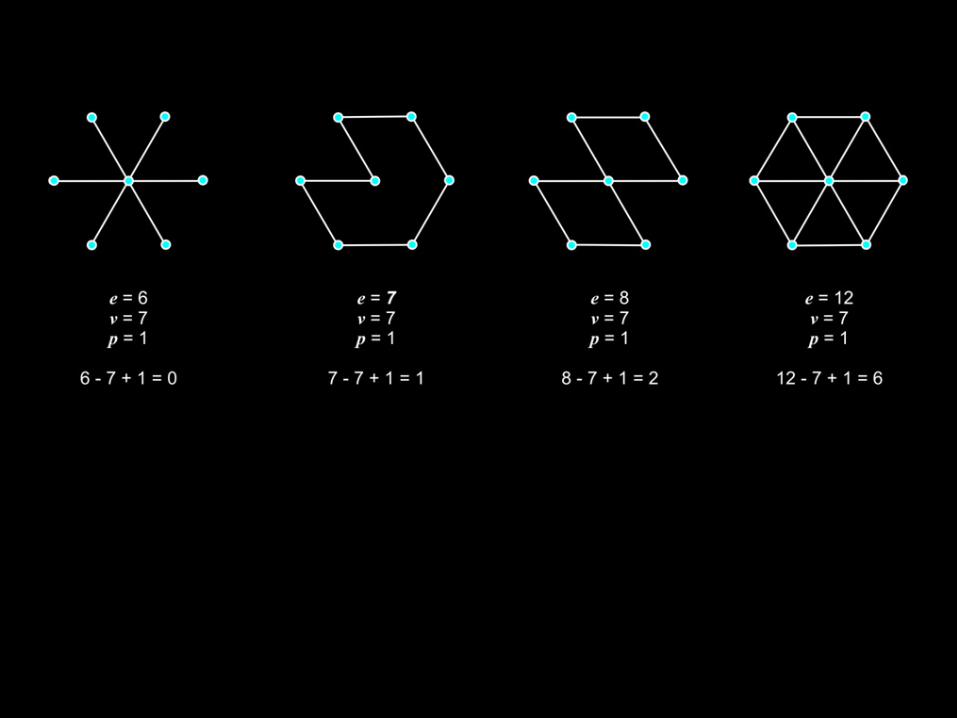
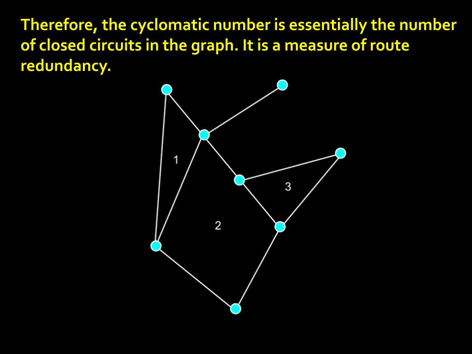
Therefore, the cyclomatic number is essentially the number of closed circuits in the graph. It is a measure of route redundancy.

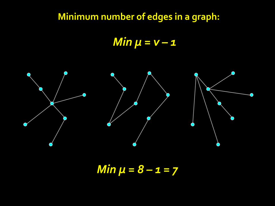
Minimum number of edges in a graph: Min μ = v – 1

Min μ = 8 – 1 = 7

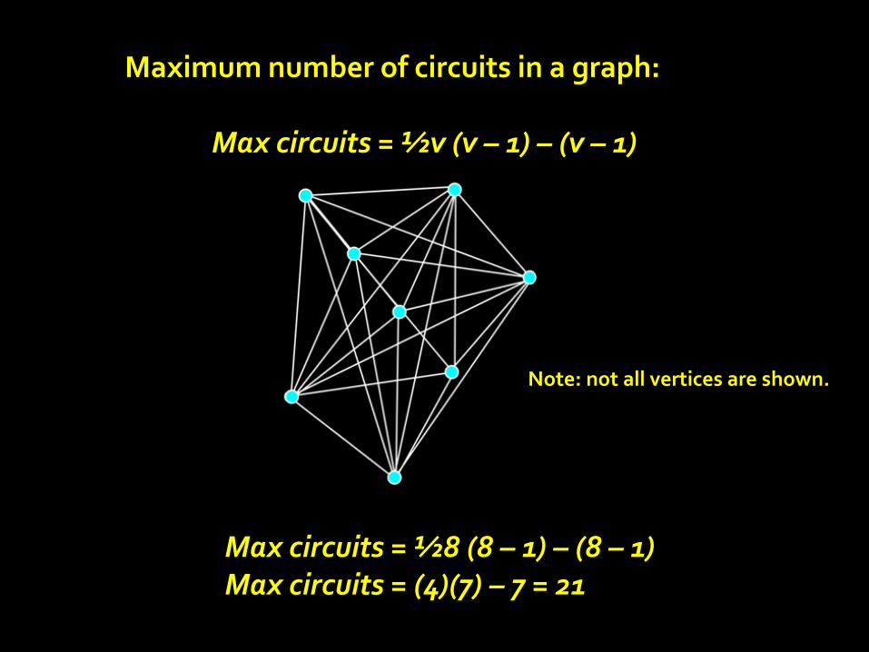
Maximum number of circuits in a graph: Max circuits = ½v (v – 1) – (v – 1)

Max circuits = ½8 (8 – 1) – (8 – 1) Max circuits = (4)(7) – 7 = 21

Note: not all vertices are shown.

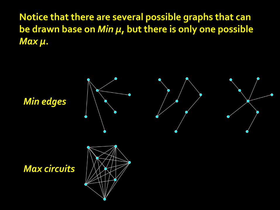
Notice that there are several possible graphs that can be drawn base on Min μ, but there is only one possible Max μ.

Min edges

Max circuits

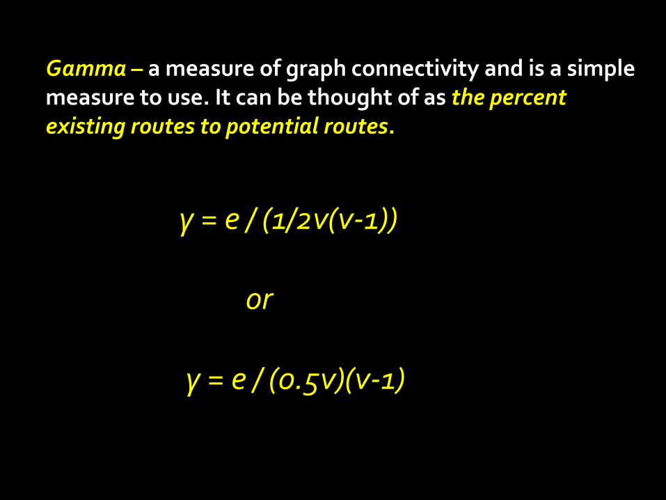
Gamma – a measure of graph connectivity and is a simple measure to use. It can be thought of as the percent existing routes to potential routes.

γ = e / (1/2v(v-1)) or γ = e / (0.5v)(v-1)

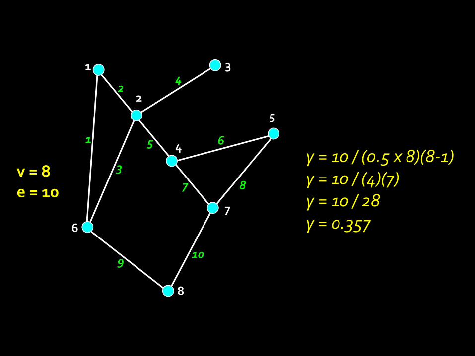
v = 8 e = 10

γ = 10 / (0.5 x 8)(8-1) γ = 10 / (4)(7) γ = 10 / 28 γ = 0.357

Remember that max μ calculates EDGES and that gamma is working with ROUTES.

Edge

Route

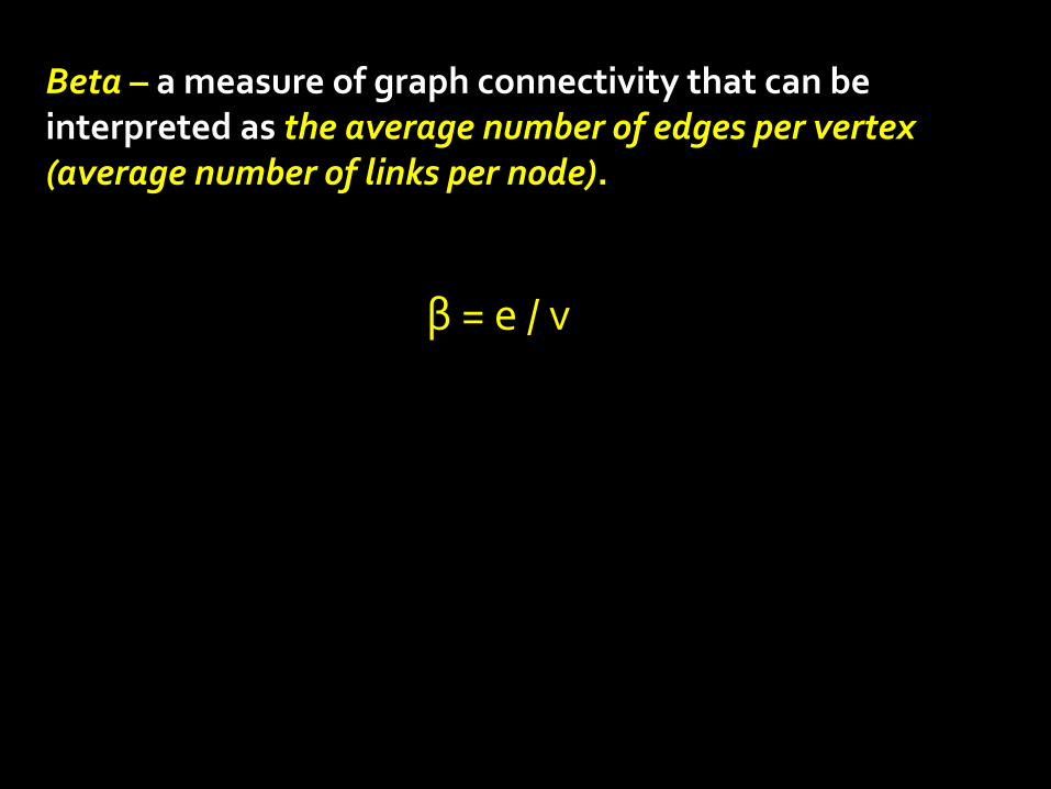
Beta – a measure of graph connectivity that can be interpreted as the average number of edges per vertex (average number of links per node). β = e / v

v = 8 e = 10

β = 10 / 8 β = 1.25

Alpha – a measure of graph connectivity that can be interpreted as the ratio of existing circuits to the maximum possible circuits. α = e – (v-1) / (0.5v(v-1)) – (v-1)

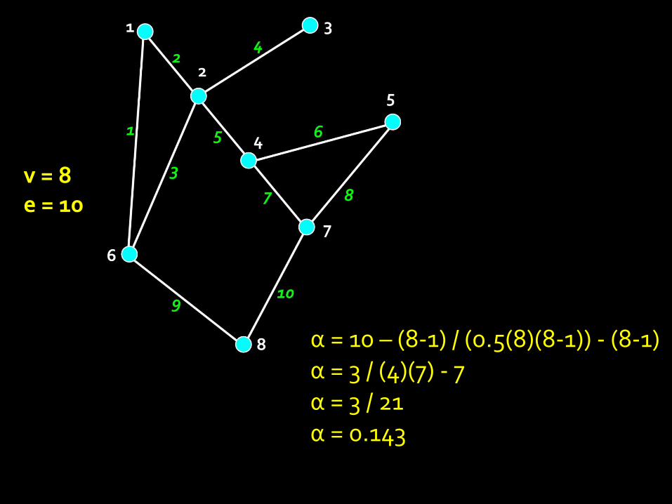
v = 8 e = 10

α = 10 – (8-1) / (0.5(8)(8-1)) - (8-1) α = 3 / (4)(7) - 7 α = 3 / 21 α = 0.143

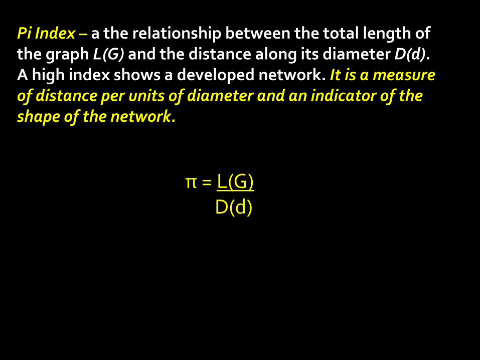
Pi Index – a the relationship between the total length of the graph L(G) and the distance along its diameter D(d). A high index shows a developed network. It is a measure of distance per units of diameter and an indicator of the shape of the network.

π = L(G) D(d)

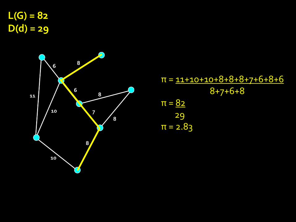
L(G) = 82 D(d) = 29

π = 11+10+10+8+8+8+7+6+8+6 8+7+6+8 π = 82 29 π = 2.83

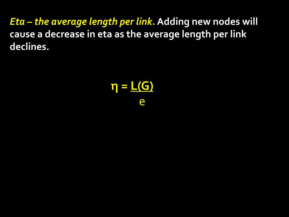
Eta – the average length per link. Adding new nodes will cause a decrease in eta as the average length per link declines.

η = L(G) e

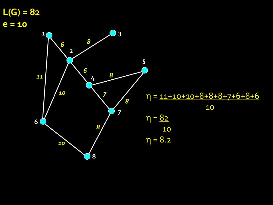
η = 11+10+10+8+8+8+7+6+8+6 10 η = 82 10 η = 8.2

L(G) = 82 e = 10

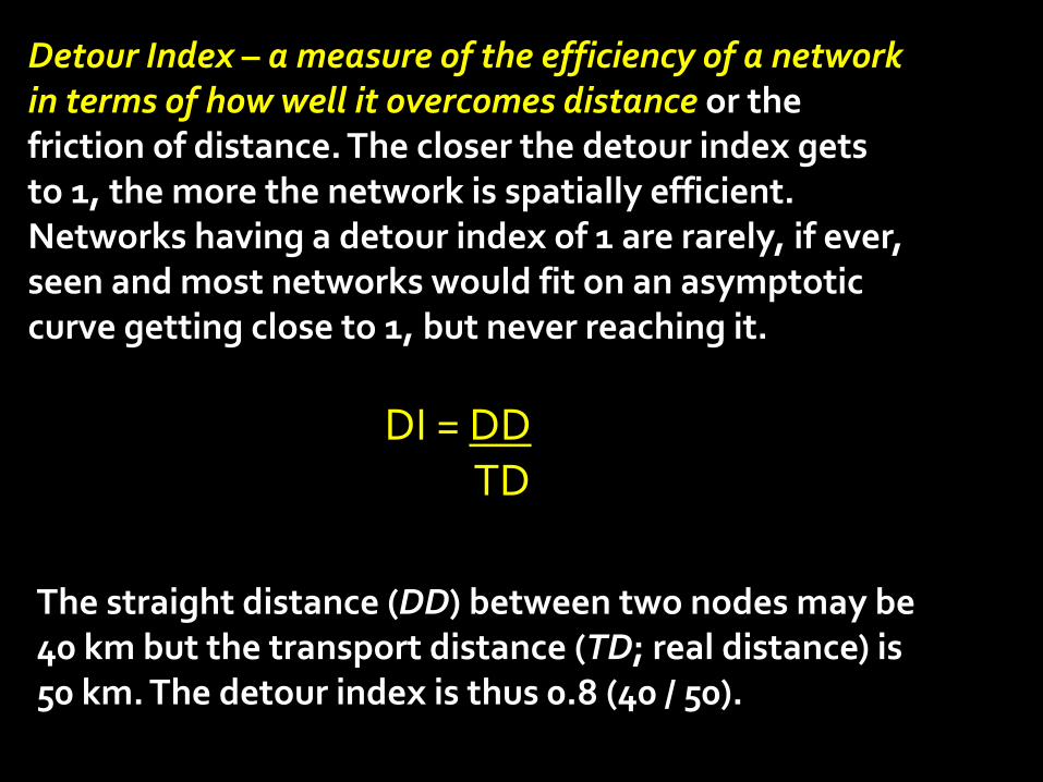
Detour Index – a measure of the efficiency of a network in terms of how well it overcomes distance or the friction of distance. The closer the detour index gets to 1, the more the network is spatially efficient. Networks having a detour index of 1 are rarely, if ever, seen and most networks would fit on an asymptotic curve getting close to 1, but never reaching it.

The straight distance (DD) between two nodes may be 40 km but the transport distance (TD; real distance) is 50 km. The detour index is thus 0.8 (40 / 50).

DI = DD TD

Transport Distance (TD) Straight Distance (DD)

DI = (10 + 11 + 10 + 8 + 9) = 48 = 0.91 (12 + 13 + 11 + 8 + 9) 53

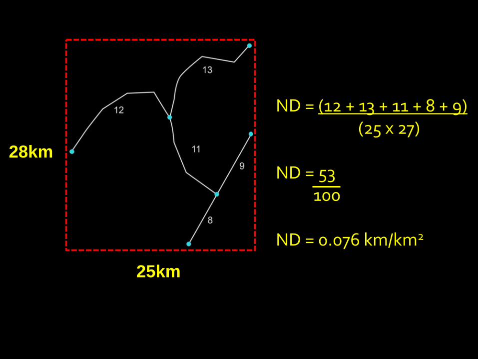
Network Density – measures the territorial occupation of a transport network in terms of km of links (L) per square kilometers of surface (S). The higher it is, the more a network is developed.

ND = L S

25km

28km

ND = (12 + 13 + 11 + 8 + 9) (25 x 27) ND = 53 100 ND = 0.076 km/km2