Transportation and Traffic Theory

Proceedings of the Eleventh International Symposium onTransportation and Traffic Theory, held July 18-20, 1990,in Yokohama, Japan

Editor

Masaki KoshiInstitute ofIndustrial ScienceUniversity ofTokyoMinato-ku, Tokyo, Japan

~&~.

~:f1~~~·".:.'."pW. ..~.~.,.~t....)...~~-.;: ..l"'l'" l'

-..~ .~ ...

ElsevierNew York • Amsterdam • London

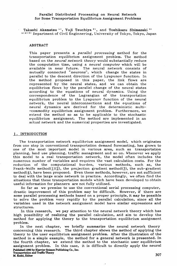
Parallel Distributed Processing on Neural Networkfor Some Transportation Equilibrium Assignment Problems

Takashi Akamatsu 1), Yuji Tsuchiya 2), and Toshikazu Shimazaki 3)

1) 2) 3) Department of Civil Enginnering, University of Tokyo, Tokyo, Japan

ABSTRACT

This paper presents a parallel processing method for thetransportation equilibrium assignment problem. The methodbased on the neural network theory" would substantially reducethe computation time, using a neural computer which will beavailable in near future. The neural network consists ofmutually connected tt neurons", which change the states inparallel to the descent direction of the Lyapunov function. Inthe method proposed in this paper, the link flows arerepresented by the neural states, apd we can obtain theequilibrium flows by the parallel change of the neural statesaccording to the equations of neural dynamics. Using thecorrespondence of the Lagrangian of the transportationequilibrium problem to the Lyapunov function of the neuralnetwork, the neural interconnections and the equations ofneural dynamics are derived for the deterministic multi­-commodity equilibrium assignment problem. Furthermore, weextend the method so as to be applicable to the stochasticequilibrium assignment. The method are implemented in anactual network and the numerical properties are investigated.

1. INTRODUCTION

The transportation network equilibrium assignment model, which originatesfrom one step in conventional transportation demand forecasting, has grown toone of the most important model in various area, such as transportationplanning, land use planning, traffic management and so on. Whenever we applythis model to a real transportation network, the model often includes thenumerous number of variables and requires the vast calculation costs. For thereduction of the computational burden, various methods, such as, theFrank-Wolfe method(!)(~), the projection gradient method(~), the sub-gradientmethod(1J, have been proposed. Even these methods, however, are not sufficientto deal with the large scale network in practice. Accordingly, we often find thesituations that these transportation models which have been developed to obtainuseful information for planners are not fully utilized.

So far as we premise to use the conventional serial processing computer,drastic· improvement of this problem may be difficult. However, if there aresome parallel processing methods based on a proper principle, it may be possibleto solve the problem very rapidly by the parallel calculation, since all thevariables used in the network assignment model have similar expressions andstructures.

In this research, we pay attention to the neural network theory which hashigh possibility of realizing the parallel calculation, an'd aim to develop themethod for applying the theory to the transportation equilibrium assignmentproblem.

In the next chapter, we briefly summarize the neural network theoryconcerning this research. The third chapter shows the method of applying thetheory to the user equilibrium assignment problem. After the illustration of themethod in a simple example, the method for a general network is presented. Inthe fourth chapter, we extend the method to the stochastic user equilibriumassignment problem. In this case, it is difficult to directly apply the neuralPublished 1990 by Elsevier Science Publishing Co., Inc.Transportation and Traffic Theory . 307M. Koshi, Editor

308

network nlethod because of the path variables included in the conventionalequivalent optin1ization problen1. Alternatively, we first develop an equivalentprogram represented by only link variables, and then we apply the neuralnetwork method to this program. In the fifth chapter, we analyse conditions ofthe stable convergence in this method. Next, we implement the method in anactual network, and investigate the numerical properties of this method. Finally,the features of the method are discussed comprehensively and the directions ofthe future research are mentioned.

2. NEURAL NETWORK THEORY

In this chapter, we briefly summarize the neural network theory, concen­trating on the themes concerning with this research. General and detailedexplanations of the theory can be seen, for example, in references(§.) -.., (11J.2.1 Model of Neuron

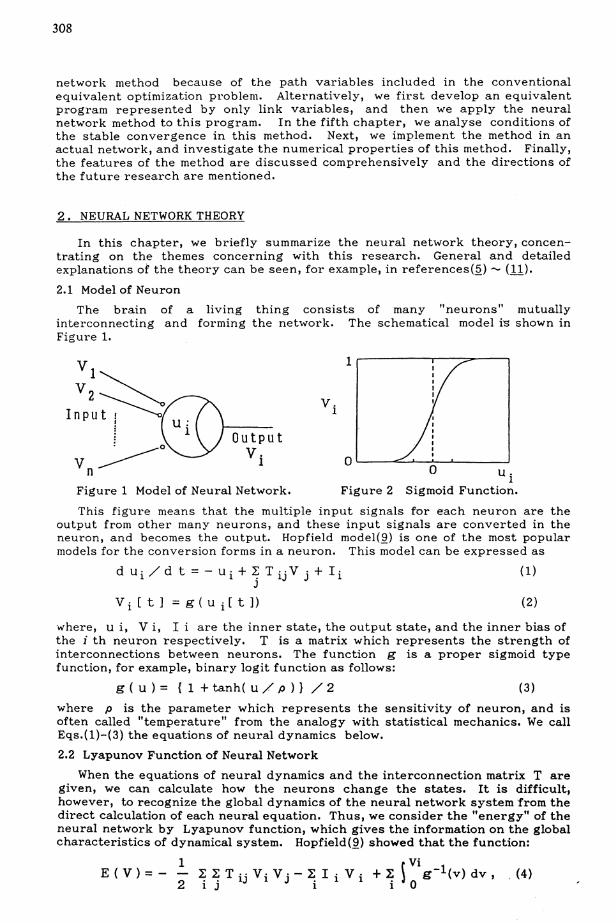
The brain of a living thing consists of many "neurons" mutuallyinterconnecting and forming the network. The schematical model is shown inFigure 1.

1

Figure 2

O'--------.&..----------Jo u.1

Sigmoid Function.

OutputV.

1

Figure 1 Model of Neural Network.

This figure means that the multiple input signals for each neuron are theoutput from other many neurons, and these input signals are converted in theneuron, and becomes the output. Hopfield model(~) is one of the most popularmodels for the conversion forms in a neuron. This model can be expressed as

d Ui/ d t = - ui + ~ TijV j + I iJ

Vi[t] =g(ui[t])

(1)

(2)

'where, U i, V i, I i are the inner state, the output state, and the inner bias ofthe i th neuron respectively. T is a matrix which represents the strength ofinterconnections between neurons. The function g is a proper sigmoid typefunction, for example, binary logit function as follows:

g ( u ) = {I + tanh( u / p )} / 2 (3)

where p is the parameter which represents the sensitivity of neuron, and isoften called "temperature" from the analogy with statistical mechanics. We callEqs.(1)-(3) the equations of neural dynamics below.

2.2 Lyapunov Function of Neural Network

When the equations of neural dynamics and the interconnection matrix Taregiven, we can calculate how the neurons change the states. It is difficult,however, to recognize the global dynamics of the neural network system 'from thedirect calculation of each neural equation. Thus, we consider the "energy" of theneural network by Lyapunov function, which gives the information on the globalcharacteristics of dynamical system. Hopfield(~) showed that the function:

E(V)=-1

2

Vi~ ~ T .. V· V · - ~ I · V· + ~ ~ g-l(v) dv Ii j IJ 1 J ill i 0

, (4)

309

is the Lyapunov function corresponding to the equations of neural dynamics(1)-(2). That is, Eqs.(l)-(2) change the state to the descent direction of E,and the stable point is the state where E is minimized. In other words, if theneurons change each input/output state asynchronously and in parallel, theneurons have the stable state at the minimum of the Lyapunov function. Notethat the third term of Eq. (4) represents randonlness arising from the continuityof the value of neural state V, and we call it "neural entropy term".

2.3 Application to Parallel Processing of Optimization Problem

According to the theory above, the neurons change their states to thedirection minimizing E ( V ) spontaneously. Therefore, an optimization problemcan be solved by changing the state of each neuron according to Eq.(l) and (2)

;in parallel, if the variables are represented by the states of neurons and theobjective function can be expressed in the fornl of Eq.(4).

Based on this idea, Hopfield and Tank(10), and Takeda and Goodmantll)showed that a class of combinatorial optimization problenl can be solved onneural network efficiently. However, the applications to the optimizationproblem of other calsses are quite sparse, since their methods for representingthe constraints in optimization problem on neural Lyapunov function are ad hocand they can not be used in general.

3. APPLYING NEURAL NETWORK THEORY TO EQUILIBRIUM ASSIGNMENTPART I : DETERMINISTIC EQUILIBRIUM PROBLEM

It is widely known that the transportation network user equilibrium problemcan be represented as the optinlization problenl when the Jacobian of the linkperformance functions is synlmetric. Therefore, if we can find out the proper"number representation" and the Lyapunov function corresponding to theassignment problenl on neural network, we nlust be able to apply the theory. Inthis research, we adopt the number representation that the link flows arerepresented by the sum of neural output states, and consider thecorrespondence between the augmented Lagrangian of equivalent optimizationproblem for the transportation equilibrium rnodel and the Lyapunov function ofneural network.

3.1 Simple Example

First, we explain the application nlethod of the neural net\vork theory to theequilibriunl assignment problenl on a simple exanlple network as shown in Figure3. The user equilibriunl assignment. problenl in this network is equivalent to thefollowing optimization problenl,

[ P 1 ]

min. Z ( X ) = ~ ~ x a C a ( w ) d wa 0

subject to

h(X)=q-LXa=Oa

.~.O~D

Figure 3 Example Network

Xa~O

where, q is the OD flow, X a is the flow on link a, and C a is the linkperformance function of link 8, which is continuous and monotonically increasingfunction.

To solve this problem by the neural network theory, we must determine howto represent the link flows Jf on neural network. Fo:rAhis "number represen­tation", we assume that the link flows are not continuous but discrete variables,that is , the link flows take integer value measured by certain unit whichrepresents number of vehicles. Next, we consider many neurons correspondingto these unit flows, and regard the output state of each neuron as the unit flow.

310

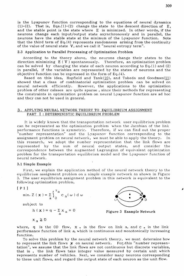
According to this "number representation" method, the link flows X arerepresented by the- sum of output states of the neurons assigned to each link;that is,

X a = L V ann

(5)

where V an denotes the output state of the n th neuron assigned on link a.Also, to represent the objective function of the equilibrium assignment problemby the discrete unit flow, we assign each neuron the value of linkperformance function, C an ' corresponding to the value of the link flowrepresented by the neuron as shown in Figure 4. As seen from Figure 4, program[Pl] can be replaced by

link cost

[ P l' ]

min. Z ( V ) = ~ ~ C an V anan

subject to

h ( V ) = q - L L V an = 0a n

V ai =1 i=l, .. ,n

= 0 i=n+l, .. ,m

C an

link flow

X a

Figure 4 Rrepresentation of Link Flow.

Since problem [PI'] is a constrained optimization problenl, we can not yetdirectly apply the idea of neural network theory. To take the constraints intoconsideration, we utilize the augnlented Lagrangian which converts theconstrained problem into unconstrained one in Inultiplier method(12):

E=Z(V)+,uh(V)+R {h(V)}2/ 2 (6)

where J..l is the Lagrange multiplier and R is a parameter of appropriate value.According to the theory of multiplier method, revising the V to the decent

direction of E by proper method, and revising ,u by

,u [t+1] = ,u [t] + R · h ( V [t]) (7)

(8)

where t. in bracket [] denotes the number of iteration,

the neural state V converges to the optimal solution of original problem.On the other hand, the Lyapunov function of this problem corresponding to

Eq.(4) is represented by

-- . 1E ( V ) = - - L L T anbm V an V bnl - L I an Van .

2 an bm an

(9)

(10)

"'\i a,n,b,nl

"'\i a,n

Letting E ( V ) - constant equals E(V), comparing the expansion of Eq.(8) andthe coefficient of Eq.(8), we obtain

T anbm = - R

I an = R q + ,u - C an

The derived matrix T means that all the neurons are mutually connected withsame "strength" R, and the neurons show "inhibitory" property. Also, theequations of dynamics for the n th neuron of link a becomes

d U an / d t = - U an + L T anbm V bm + I anbm

= - U an + R (q - lm V bm) + f.l - C an I

(11)

(12).'

311

V an [ t ] = { 1 + tanh ( U an [ t ]/ p )} / 2 • (13)

Thus, if we connect the neurons mutually according to the interconnectionmatrix T on a neural network computer, the neurons change the statesaccording to the equations 'of dynamics (12)(13) spontaneously, and we canobtain the user equilibrium flow pattern as the equilibrium state of the neurons.

To check this fact numerically in conventional digital computer, the equationsof dynamics (12) should be replaced with the following discrete-time differenceequations.

(14)U an [ t ] = R { q - L V bm [ t - ~ bm]} + j.J. - C anbm

where Il bm is the time-interval of changing the state of the bm th neuron.

Note that the temperature parameter p at equilibrium should be taken as verysmall value for the consistency of the analysis, since we derived the equationsof dynamics assuming that the neural entropy term of the Lyapunov function canbe dropped because it is negligibly small. For this reason, we adopt the methodanalogous to the simulated annealing method (13), that is, p is first set highvalue and then p is "cooled" down gradually and finally decreased to the levelthat the entropy ternl can be regarded as zero. Detailed discussion on therelation between the value of this temperature parameter /J, the penaltyparameter R and the convergence condition will be shown in the fifth chapter.Here, we can demonstrate the simple numerical experiment of the method ondigital computer,. revising p by

p = p max / log ( t + 1 ) ( t ~ 1 ) , (15)

where p max : a constant of given positive value; t : number of iteration,

and changing the state of neurons according to Eq. (7) ,( 14), and (12). Someconditions of the numerical experiment are as follows:

ill Number of links : 2 ;~ OD flow : 20.0;

@ Link performance function : c 1 = 200 + 0.02 X t ' c 2 = 300 + 0.15 X ~

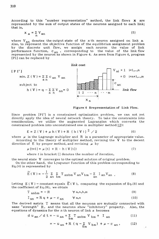
@ Value of temperature parameter : p max=100;® Value of penalty parameter R = p / 2@ Initial state of the neurons: V an [0]= o. 5 V an

Cl Cl Cl

Xl Xl XlFigure 5 (a) t=l (b) t=3 (c) t=10

Figures 5 (a)-(c) show the changes of neural states in link 1 to the convergence.The width of each bar means the unit link flow represented by one neuron, andthe ratio of the hight of shaded area against the bar represents the value ofoutput state (from 0 to 1) of each neuron. We can see that initially randomvalued neurons gradually converge to the ordered state of user equilibrium.

3.2 Analysis in General Network with Many to Many OD pairs

We extend the previous analysis for the one OD pair problem to the generalnetwork with many to many OD pair. The equivalent optimization problem of user

312

equilibrium assignment in this case can be represented by

x· .r IJmin. Z ( X ) = ~. J C ij ( W ) d w

IJ 0subject to

(16)

-- s s s s·h k (X ) = q ks + ~ X ik - ~ X kj = 0

1 J

g .. (X, X s) = X .. - L X~· = 0IJ . . IJ S IJ

SX ij ~ 0

V'k;ts

V' (ij)

V' (ij), s

(17)

(18)

(19)

where q ks is the OD flow from node k to node s, X ij and C ij denotes the

flow and the performance function of link i ~ j, respectively, and X fj denotesthe flow with destination s on link i ~ j. As in previous section, we representthe link flows by the sum of the activated (output) state of neurons. Also, inorder to express the flow conservation constraints on the neural network, weconsider two groups of neurons, V ':), V:s, corresponding to the link flows, X,and the link flows with destination s , X S ,respectively. The link flowswithout distinguishing destinations are represented by

(20)V' (ij)X·· = L V·~IJ n IJn

and then the objective function Z can be represented as the function of V.

Z(X)=Z(V)=LLij n

oC ijn V ijn (21)

where C ijn denotes the value of the link cost function at X ij = n (unit flow).

Also, the link flows with destination s, X s ,is represented by

X?· = L V!3·IJ n IJn

and then the constraints 11 can be transformed into

V' s, (ij) (22)

(23)s s s

h k ( V ) = q ks + ~ L V ikn - ~ L V kjn = 0 V' s, k1 n J n

Furthermore, to satisfy the constraints g, we introduce next constraints for V '":'and V 5.

o sg ijn ( V ) = V ijn - L V ijn = 0

s;tOV' (ij), n (24)

Consequently, the augmented Lagrangian for this problem can be representedwith respect to V = ( V 0,.. , V :s ,.. ) as follows:

(25)

E = Z ( V ) + L L jJ. ~ h ~ ( V) + ~ L Aijn g ijn ( V )s k IJ n

+~ ~ ~ { h k(V ) } 2 +~ ~. ~ {g ijn ( V ) } 22 s k 2 IJ n

where JJ. and ~ are the dual variables corresponding to the constraints handg, respectively. On the other hand, the Lyapunov function of this problemcorresponding to Eq.(4) becomes

1 ss' s s' s sE = - - ~ ~ L L ~ L T iJ'ni'J"n'V iJ·n V i'J"n' - L L L I iJ'n V iJ'n (26)

2 ij n si'j' n' s' ij n s

where E ( V ) is E ( V ) - constant.· Comparing the expansion of Eq.(25) and the

(27)

313

coefficient of Eq.(26), we obtain the interconnection matrix, T, and the vector ofneural threshold value, I.

(i) Case for s = 0

ss'T ijn,i'j'n' = R 2 ( 1 - 2 0s'O ) 0ii' ~j' 0nn'

sI ijn = - C ijn - A ijn

(ii) Case for 5 # 0

ss'T ijn,i'j'n'= RIo ss' ( 0 ij'+ 0 ji'- 0 ii' - 0 jj')

- R 2 ( 1 - 2 0s'O) 0ii' Ojj' 0nn'

s s sI ijn = R 1( q is - qjs) + A ijn + ( J.1. i - J.1. j )

where 0 denote Kronecker's delta; that is,

(28)

(29)

(30)

= 1= 0

if x = y

otherwise.

We can see from the derived matrix T that the n th neuron assignned for x IJhas the interconnections between the n th neurons for the link flows withdestinations 5, X ij' corresponding to the constraints g in the case of (i).In the case of (ii), the interconnections have the structure similar to the dualgraph of the original transportation network, corresponding to the flowconservation constraints h.

Substituting the nlatrix T and the vector I into the basic equations ofdynamics, we can derive the follow~ng equations of dynamics.

s . sV ijn [ t ] = { 1 + tanh( U ijn[ t ] / p )} / 2

(0 case for 5 = 0 (neurons for link flows)

(31)

d u Sijn / d t = - u tjn - { C ijn + A ijn + R 2 g ijn ( V )} (32)

(ii) case for 5 ~ 0 (neurons for link flows with destination s )

s s s sd U ijn / d t = - U ijn + ( J.1. i - J.1. j) + A ijn

+ R 1{ h f (V ) - h j (V )} + R 2 g ijn ( V ) (33)

In order to see the interconnection between neurons, we derived the matrix Tby comparing the coefficients, and then obtained the equations of dynamics bysubstituting the matrix T into the basic equations of neural dynamics. Note thatthe equations of the dynamics can be also obtained by merely differentiatingEq.(25) with respect to V, since the neural equations represent the dynamics tothe descent direction of the Lyapunov function.

4 • APPLYING NEURAL NETWORK THEORY TO EQUILIBRIUM ASSIGNMENTPART II: STOCHASTIC EQUILIBRIUM PROBLEM

4.1 Equivalent Optimization Problem

In this chapter, we develop the neural network method for solvingstochastic user equilibrium (SUE) model which is known as a generalization ofdeterministic user equilibrium (e.g.(14)-(17». From the practical view point, weconcentrate on the case for logit type path choice model below. Conventionally,the minimization problem developed by Fisk(15) has been known as an equivalentprogram for the logit based SUE assignment model. The program, however,includes the path flow variables which are troublesome to deal with in general

(34)

(35)

314

network, and it is difficult to directly apply our neural network method by thesimilar manner in earlier deterministic equilibrium case. Thus, alternatively, wederives the equivalent optimization problem represented by only link flows, andapply the neural network method to the link based program.

To show the essence of "decomposition into link based program" withoutnotational complexity, we first consider the case for flow independent stochasticassignment problem with one OD pair and unit OD flow.

In the logit type stochastic assignment model, the probabilities of choosingpath p, Pp, is given by

exp r - e c p ]P =

p L exp [ - e c p' ]P'

where e is the dispersion parameter for path choice, and C p is the travel costof path p , which is the sum of the link cost t on the path. The probability(flow) of choosing link i ~ j, P ij , is determined by the flow conservationequations represented by the link and path flows:

P ij = ~ P p 0 ij,p ,

wheI"e {=1: if link i ~ j is on path p,oij,p =0: otherwise.

The flow pattern obtained by this assignment model has the property of "Marcovchain"; that is,

IT [prOb[i' j] ] 0 ij,p = P

ij Prob[j] p

where Prob[j] = L Pmj' Prob[i, j] = Pij ·ID

In other words, if a certain link flow pattern satisfies

(36)

ITij [ L Pmj

m

] 0 ij,p = exp [ - e C p ]

L exp [- e c p']p'

(37)

then the flow pattern is consistent with the logit type assignment model.Keeping in mind the above property of logit based stochastic assignment

model, let's consider the following program:

[SA]

min. Z ( p) =1

e{ LP" In P 0 0 - L ( L P 0 0 ) In ( ~ P ij )} + L Pij C ij

ij IJ IJ j i IJ 1 ij

subject to

L P ik - L P kJo + (0 rk - 0 sk) = 0 'V ki j

P ij ~ 0 't ij

where r is the origin and s is the destination node.

The solution of this problem has the property of Marcov chain, and the resultinglink flow pattern is identical to those obtained by logit type assignment model(Eq.(34)(35)). In other words, this program is equivalent to the logit typeassignment model in terms of the link flow pattern~ The equivalency can beshown by comparing the optimality conditions of this program and the propertiesof Marcov chain mentioned above (Eq.(37». Using the Lagrangian, which isgiven by

L(p, ,u)=Z(p)+LkfJ.k {~Pik-~Pkj+(ork-osk)}'(38)1 J

315

we can express the optimality conditions for program [SA] as follows:

a L---~O,

a Pij

aLP ij = 0 ,

a P ijV'ij (39)

(40)V' ij= exp [ - e {c .. - ( j.J. • - j.J. .)} ] •IJ 1 J

and the flow conservation constraints.

After some algebraic calculation, the optimality conditions Eq.(39) yield

P ij

L Pmjm

Multiplying the both side of Eq.(40) on appropriate path p,

I1 I P ij I<5 ij,p = IT exp [- e {c ., - (J.L .- J.L .)}] <5 ij,p (41)ij L P ij IJ 1 J

m rnj

=...exp [ - e {c p - ( j.J. r ~ J.1. s )} ] (42)

Furthermore, considering the flow conservative in Eq.(40), we have

exp[ e j.J. j ] = ~ {exp[ - e C ij ] exp[ e f.J. i]} ·1

(43)

Eq.(43) shows that the value of f.J. at node j is determined by the value of J.1. atnode i which has links entering to node i ( in other words, nodes i are justpreceeding to node j). Thus, sorting all the node from destination s to origin rby appropriate order ( s,s-1,s-2,· .. ,1"+2,1'+1,1') and evaluating the value of jJ.

on this order of node reversely,

exp[ () f.J.s ] = L {exp[ - e Cs-I s ] exp[ e }.ls-1 ]}s-1 '

= L {exp[ - e C s-1 s] L exp[ - e c s-2 8-1 ] . · · .. X exp[ e }.l r]}s-1 ' s-2 '

= L L" L exp[ - e ( c s-1 8 + c 8-2 8-1 + .. + c 1'+1,1'] X exp[ e }.l l' ]s-1 s-2 1'+1 "

L exp[ - e C pJ X exp[ e f.J.1.Jp

(44)

Hence,

(45)j.J. r - j.J. 8 = - ( 1 / e ) In L [ - e C].)] ·p

Substituting Eq.(45) into Eq.(42), we have Eq.(37) as the optinlality condition forthe program [SA]. This means that we can obtain the link flo\v pattern consistentwith logit model by solving the program [SA].

Similarly, we can obtain an equivalent program for SUE with many to rnany ODpairs represented by only link variables as follows:

1 x ..min. Z ( X ) = - L { - H L + H N } + L r· IJ C iJ' ( w )d w (46)e s s s ij J 0

subject to

Eq.(17), Eq.(18), and inequalities (19),

where H Ls ( X s ) == - L X ~. In x!3· ·ij IJ IJ'

HNs(xs)= -L(Lx~·)ln(Lx~,).

j i IJ i IJ

(47)

(48)

316

4.2 Deriving the Equations of Neural Dynamics

In order to apply the neural network method, it is rather convenient toconvert the entropy term in the objective function Z into the following"conditional entropy" form:

L { - H L s + H N s} = L { L ( L X ~ , ) (L p ~, In p~.)}s s j i 1J i 1J 1J

ss ~ P ij s= L { L ( LX·· ) L ( 0 In w d w + P ij)} (49)

s j i 1J i

wheres s s

P ij == X ij / ~ X ij ·1

·(53)

As in deterministic case, we represent the link flows by the sum of theoutput state of neurons. In addition to the neural variables V = (V '-:> , •• , V :s , •• )

in deterministic equilibrium case, we further introduce a new set of neuronsrepresenting the "turn probabilities", p, as follows:

~ V s 1 S (£;0)~ ijn = P ij vn

where the superscript "1 " denotes this set of neurons, and the other types ofneurons representin,g the link flows are distinguished by superscript" 0" belo"v.From the definition of p and the other neuron variables representing the link

flows, these variables should satisfy the following equations.

s sI sa s s sf,· (V 1'J'., V 1'J") == XI'J' - P " LX"1J 1J i 1J

sa sl sa=L V ijn - ( L V ijn )( L: L: V ijn) = 0 (51)n n i n

Similar to the discrete representation in the integral ternl of the link costfunction, we can express the integral of the entropy term by

ss . J P ij sa s 1 . r-

L ~ (~Xij )( ~ In w d w ) = L L, ( ~ 2: V ijn){ ~ L L n V ijn}' (~2)s J 1 1 0 s J In 1 n

where L n denotes the value of function In(') corresponding to the n th

division of the interval [0,1]. Consequently, we have the following augmentedLagrangian with respect to V, adding the constraints Eq.(51) and the entropyterm to those of the deterministic equilibrium case.

sO sIE = ~, L Cijn V ijn + L ~ ( ~ L: Vi'jn){ L ( 1 + L n ) V ijn } / e

1J n s IJ l' n n

s s s s+ LL,uk,hk(V) +,~LAijngijn(V)+L,~lIijf,· (V)s k IJ n s IJ 1J

+~1 L L { h 1( V ) }2 +~ ~. L { g ijn ( V ) } 22 s k 2 IJ n

where }J., A and 11 are the dual variables corresponding to the constraints h,g, and f, respectively. On the other hand, the Lyapunov function of thisproblem corresponding to Eq.(4) becomes

1E= ss'dd' sd s'd'

L L L L ~ ,L 2 L T iJ'ni'J"n' V iJ'n V i'J"n' - L L 2 L2 ij n s d l'J' n' s ' d ' ij n s d

sd sdI ijn V ijn

(54)

317

Similar to the deterministic equilibrium case, we obtain the followinginterconnection matrix, T, and the vector of threshold value, I.

ss'dd'T ijn,i'j'n'= 0 dO 0 d'O (0 sO {R 2 ( 1 - 2 0 s'O) 0 ii' 0 jj' 0 nn'}

+ (1-os0){-R 2 (1-2<;'0 )oii' ~j' 0nn'

- RI 0 ss'( 0ij' + 0 ji' - 0 ii'- 0 jj")})s

- 0dOod'lo jj'O ss'( 1 - 0sO) (1 + L n ,- }/ij )/8 (55)

sd· s s sI ijn = 0 dO ( ( 1 - 0 sO ){ R 1 ( q is - q js) + A ijn + ( jJ. i - jJ. j ) - 11 ij }

- 0 so ( C ij n + A ijn) ) (56)

The first line of Eq.(55) means the interconnection of the neurons for s=O (theneurons representing link flows), the second line is those for s :# 0 (the neruonsrepresenting link flows with destination s), the third line is common to all theneurons excluding "turn probability neurons", and the last line shows theconnection for the "turn probability neurons".

Substituting the matrix T and the vector I into the basic equations ofdynamics, we can derive the following equations of dynamics for three types ofneurons.

sd sdV ijn [ t ] ={1 + tanh( U ijn [ t ] / p )} / 2 (57)

(i) case for s = 0 and d = 0 (neurons for link flows}

s d s dd U ijn / d t = - U ijn - { C ijn + A ijn + R 2 g ijn( V )} (58)

lliLcase for s;t:. 0 and d = 0 (neurons for link flows with destination s )

sd sd s s sd U ijn / d t = - U ijn + ( j.J. i - j.J. j) + A ijn - }/ ij

+R1{hf(V)-h j(V)} +R 2 gijn(V)

+ { 1I's. - L - 1 } L L V?~ / e (59)IJ n i n IJn

(iii) case for d = 1 (neurons for "turn probabilities")

s d s d s sOd U ijn / d t = - U ijn + ( 11 ij - L n - 1 ) ~ L V ijn / e (60)

1 n

Thus, . we know that the stochastic equilibrium flows can be calculated on neuralnetwork, by simply connecting the neurons according to the derived matrix Tand changing the neural states, as in deterministic case.

5. STABILITY ANALYSIS

Replacement of the continuous-time differential equations (Eq.(12» with thediscrete-time equations (Eq.(14» sometimes causes the unstable dynamics ofneurons, depending on the value of parameter p and R. Thus, this chapteranalyses the conditions that the equations of dynamics always converge to theequilibrium solution. To avoid the notational complexity, we analyse 1 OD pairproblem here, which is expressed by the following equations of dynamics.

V an[t+l] = gan[ V [t]] == g [ U an ( V [t])] (61)

318

where-1

g ( U an) = [ 1 + exp( - 2 U an / p )]

U an = R · ( q - L V bm ) + J.1. - C anbm

(62)

(63)

In the case for many to many OD pairs, the basic way of analysis is same as theone OD pair case, though the neural equations corresponding to Eq.(62) becomesmore complicated.

Suppose that V (t) are at the equilibrium state V *, and that the output stateof the n th neuron of link a is changed to V a n* + Can. Since V * satisfies theflow conservation, the output state at time t+ 1 becomes

-1V an [t+1]=[1+M·exp(-2c an R/p)], (64)

where M == exp{( J.1. - c an )/ p}. (65)

On the other hand, the condition for stable convergence may be expressed asfollows:

I V an [t+l]-V an [t] 1< 1 canl, (66)

Substituting Eq.(64) into Eq.(66) and rearranging ( R, p, M > 0 ) it, we have

1 - C an ( 1 + 1 / M )( 1 + M · L) < L

where L ==exp( - 2 canR/ p).

(67)

(68)

Taking the logarithm of both side, expanding by progression, and neglecting thehigher order term, we have

2R/p «I+I/M)(I+M·L). (69)

Since E an is small enough, we can see L = 1, and then the right hand sidehave the minimum value of 2 p at M = 1 (J.1. = Can) • Hence, the illost strongcondition for convergence is expressed as p > R / 2 .

Generalizing the analysis above, we can obtain the following conditions forconvergence based on the contraction mapping· theorem.

I1 Jg(V) 11 < 1, (70)

where J g ( V ) is Jacobian of g ( V). If we assume the changing ratio of J..land the distribution of neural states V, we can derive the convergenceconditions for general case from Eq.(70). However, this condition is too strongfor the practical calculation, since we do not have to consider the extreme casethat all the neurons always converge. Besides, we do not always need the linkflows by OD pairs X:S, but rather need the link flow without distinguishing ODpairs x. Therefore, we may be able to achieve the convergence according tomore weak conditions in many cases. Unfortunately, the analytical derivation ofthe weak convergence condition in general case would be extremely complicated,and the practical assumption on the distribution of neural states is not clear.Thus, we investigate the convergence properties of this method by somenumerical experiments in the following chapter.

6. NUMERICAL EXPERIMENTS

We apply the method of neural network (we call it MNN below) to solve theuser equilibrium assignment problem in practical size network, and the accuracyof the solution and the convergency of the method are investigated in thisnumerical experiment.

We implement the method in a road network of Sioux Falls city in SouthDakota, which has 76 links, 24 nodes (all the nodes are OD nodes), and 529 ODpairs. The network is same one where Leblanc et al (1) investigated theperformance of Frank-Wolfe method for solving the fixed demand user

319

equilibriunl assignment problem, and the OD flows and the link performancefunction paranleters are the same as the Leblanc's experiment.

The conditions in MNN are summarized as follows:

CD Number of neurons per link: 30@ Revising equation of temperature parameter p : Eq.(15) , p max = 10.0@ Revising equations of penalty parameter R. i (i=1,2):

Ri = R max - A X t, R max = 15.0, A =0.01

@ Revising equations of Lagrange nlultipliers:

j.J.~ [t+l] = j.J.~ [t] + R 1· h k(V[t]) (71)

A ijn [t+l] = Aijn [t] + R 2 · g ijn ( V [t]) (72)

(ID Equations of neural dynanlics: Eq.(31),(32),(33)

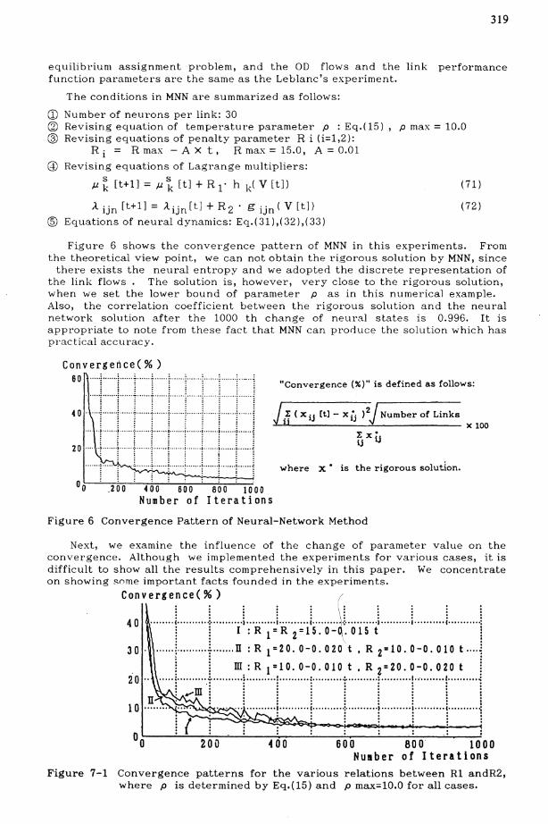
Figure 6 shows the convergence pattern of MNN in this experiments. Fromthe theoretical view point, we can not obtain the rigorous solution by MNN, since

there exists the neural entropy and we adopted the discrete representation ofthe link flows. The solution is, however, very close to the rigorous solution,when we set the lower bound of parameter p as in this numerical example.Also, the correlation coefficient between the rigorous solution and the neuralnetwork solution after the 1000 th change of neural states is 0.996. It isappropriate to note from these fact that MNN can prociuce the solution which haspractical accuracy.

where x· is the rigorous solution.

Convergence( % )

:: .. ::·::,:·::·::,::::::;:::·::1::·:::1:::::::'::··:::1:::::::1::·::::1::-'::1 ·j'i;~n~:r::~c: :j%:~jSN:::::do::::::W

::100......! ! ~ ~ ! ! ! ~ ? { 1: x •

: : : : : : : : : : ij ij

20 ··r·······l······t······t······I·······!······"!"······! , j.......!..... ~ ··~···· .. ·~·· ..··;···· .. ·;· .. ···T······~····· ..~······1

°0 .200 400 600 800 1000Number of Iterations

Figure 6 Convergence Pattern of Neural-Network Method

400200 600 800' 1000NUlber of Iterations

Figure 7-1 Convergence patterns for the various relations between RI andR2,where p is determined by Eq.(15) and p max=10.0 for all cases.

Next, we examine the influence of the change of parameter value on theconvergence. Although we implemented the experiments for various cases, it isdifficult to show all the results comprehensively in this paper. We concentrateon showing sonle important facts founded in the experiments.

convergejce(~) i i ! (i j i i i40 ········r·· ·r· i·I·:..ii..~·~·R··~·~·i'5·:·ii·~·\·ii·i·S ..t ··..·· ..· ·· I !30· ~ + n: R 1=20.0-0.020 t • R 2=10.0-0.010 t ~

! 1 m.:R1=lO.O-O.OlOt,Rz=ZO.O-o.OZOt 120 .. . ~ i···········~ i········ .. ~ ! ~ ~ i··········i

: ~m ~ ~ ~ ~ ~ ~ ~ i !· ..: ..........j..·....·.. j..........t· ..·..·..·j·........·\"..·....·j· ..........j

320

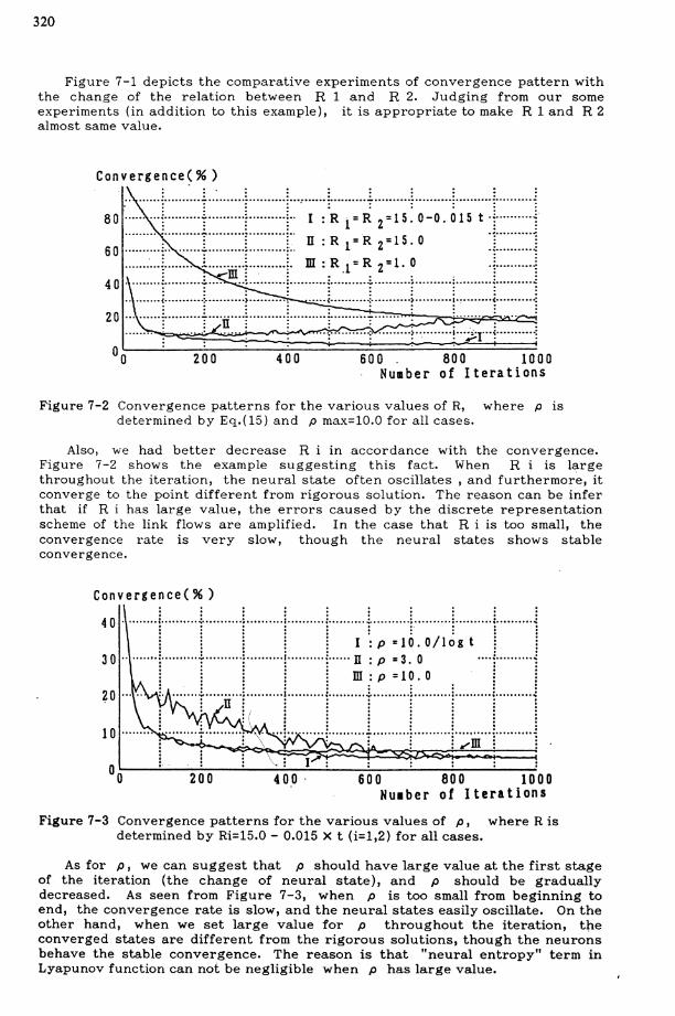
Figure 7-1 depicts the comparative experiments of convergence pattern withthe change of the relation between R 1 and R 2. Judging from our someexperiments (in addition to this example), it is appropriate to make R 1 and R 2almost same value.

Convergence(% )

600. 800 1000Nu.ber of Iterations

400200

· .· .· . . . . . . . . ... ······:··········7··········:··········:···~······:··· --:- : : : e:

80 : ~ ~ ? ~.. I :·R 1" =R2=15 : 0-0. 015 t .~ ~.· . . . . .60 :::::::::.;::··::::::t::::::::::(:::::::t: n: R 1=R 2=15 · 0 :j::::::::::~

4 0 :.:::::::: l::::::::··~ :::: ·iii::~::::::::::I:· ..~..~ r:~~·~ .~:.~.'..; ;.. ·······:1::::::::::~......... ~ ~ ? ; ( ~ ~ !.~ ~ ~

20 ······~··········f····ii····~··········~··········~··· ~ ~ :........ ~ :. .' . . ~ ';' ~ ..: ! ';;:1". ~ e •• ':

Figure 7-2 Convergence patterns for the various values of R, where p isdetermined by Eq.(15) and p max=10.0 for all cases.

Also, we had better decrease R i in accordance with the convergence.Figure 7-2 shows the example suggesting this fact. When R i is l~rge

throughout the iteration, the neural state often oscillates, and furthermore, itconverge to the point different from rigorous solution. The reason can be inferthat if R i has large value, the errors caused by the discrete representationscheme of the link flows are amplified. In the case that R i is too small, theconvergence rate is very slow, though the neural states shows stableconvergence.

Convergence(% )· . . . . . . . . .· . . . . . . . . .· . . . . . . . . .40 . ········i··········i···········~··········~··········~··········t··········~···········;··········i··········i

~ ~ ~ ~ ~ I': p =10. 0 / log t ~ i30 .. ·······i···......·+··········f··········i··········;······ n : p =3. 0 ····i··········1

: : : : : m·p=10.0 ::: : : : : :. : : : :: •••••• ·.·:. ••••••••• ·; •••••••••• 1•••••••••• : •••••••••• .:,. ••••••••••: •••••••••• : •••••••••• : •••••••••• .:

! n j I 1 1 1 1 ! I10 . ..: : .:. : : : .:

: : : ; ~ ~m i i

200 400 600 800 1000Nu.her of Iterations

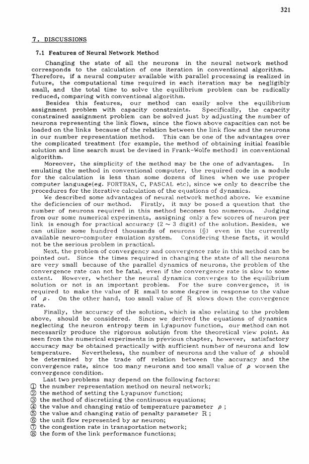
Figure 7-3 Convergence patterns for the various values of p, where R isdetermined by Ri=15.0 - 0.015 X t (i=1,2) for all cases.

As for p, we can suggest that p should have large value at the first stageof the iteration (the change of neural state), and p should be graduallydecreased. As seen from Figure 7-3, when p is too small from beginning toend, the convergence rate is slow, and the neural states easily oscillate. On theother hand, when we set large value for p throughout the iteration, theconverged states are different from the rigorous solutions, though the neuronsbehave the stable convergence. The reason is that "neural entropy" term inLyapunov function can not be negligible when p has large value.

321

7. DISCUSSIONS

7.1 Features of Neural Network Method

Changing the state of all the neurons in the neural network methodcorresponds to the calculation of one iteration in conventional algorithm.Therefore, if a neural computer available with parallel processing is realized infuture, the computational time required in each iteration may be negligiblysmall, and the total time to solve the equilibrium problem can be radicallyreduced, comparing with conventional algorithm.

Besides this features, our method can easily solve the equilibriumassignment problem with capacity constraints. Specifically, the capacityconstrained assignment problem can be solved just by adjusting the number ofneurons representing the link flows, since the flows above capacities can not beloaded on the links because of the relation between the link flow and the neuronsin our number representation method. This can be one of the advantages overthe complicated treatment (for example, the method of obtaining initial feasiblesolution and line search must be devised in Frank-Wolfe method) in conventionalalgorithm.

Moreover, the simplicity of the method may be the one of advantages. Inemulating the method in conventional computer, the required code in a modulefor the calculation is less than some dozens of lines when we use propercomputer language(eg. FORTRAN, C, PASCAL etc), since we only to describe theprocedures for the iterative calculation of the equations of dynamics.

We described some advantages of neural network method above. We examinethe deficiencies of our nlethod. Firstly, it may be posed a question that thenumber of neurons required in this method becomes too numerous. Judgingfrom our some numerical experinlents, assigning only a fe",,' scores of neuron perlink is enough for practical accuracy (2 -- 3 digit) of the solution..Besides, wecan utilize some hundred thousands of neurons (§) even in the currentlyavailable neuro-conlputer emulation system. Considering these facts, it wouldnot be the serious problem in practical.

Next, the problenl of convergency and convergence rate in this nlethod can bepointed out. Since the times required in changing the state of all the neuronsare very small because of the parallel dynamics of neurons, the problenl of theconvergence rate can not be fatal, even if the convergence rate is slo\\I to sonleextent. Ho\vever, whether the neural dynanlics converges to the equilibriumsolution or not is an inlportant problem. For the sure conver,gence, it isrequired to make the value of R snlall to sonle degree in response 'to the valueof p. On the other hand, too snlall value of R slows dow"n the convergencerate.

Finally, the accuracy of the solution, which is also relating to the problenlabove, should be considered. Since we derived the equations of dynamicsneglecting the neuron entropy term in ~apunov function, our method can notnecessarily produce the rigorous soluti n from the theoretical view· point. Asseen from the numerical experiments in p evious chapter, however, satisfactoryaccuracy may be obtained practically wi~ 1 sufficient number of neurons and lowtemperature. Nevertheless, the number of neurons and the value of p shouldbe determined by the trade off relation between the accuracy and theconvergence rate, since too many neurons and too small value of p worsen theconvergence condition.

Last two problems may depend on the following factors:CD the number representation method on neural network;® the method of setting the Lyapunov function;@ the method of discretizing the continuous equations;@ the value and changing ratio of temperature parameter p@ the value and changing ratio of penalty parameter R;® the unit flow represented by ar neuron;GJ the congestion rate in transportation network;@ the form of the link performance functions;

322

® netwTork scale( number of links, nodes, OD pairs etc.), andaID network structure.

First three factors (CD........, @) are concerned with the formulation of theproblem. The next threes (@........, ®) are the problem of relation betweenparameter value and convergency, and the remainings ((J)........, aID) are theproblem of "congeniality" between the properties of network and the methodwhich has been also discussed in conventional algorithm.

7.2 Correspondence between Neural Network Method and Other Theories

The features of MNN considered in this paper are summarized as follows:CD link flows are treated as the set of the discrete unit trip by the neurons;@ the discrete neuron variables are processed in parallel;@ Lyapunov function of neural network coincides with the augmented Lagrangianof assignment problem;@ Lagrange multipliers are revised according to the theory of multiplier method,

In examining these features, we can see the characteristics common to thetheory for other problem. In relation to CD and @, We might think of therelation with the "cost - efficiency theory" by T.E.Smith(18). He has derivedthe user equilibrium assignn1ent from the consideration in the case that networkflows are represented as discrete variables. Since our MNN represents the linkflows as the discrete variables by many neurons and both theory of the neuralnetwork and cost-efficiency have common methodology similar to statisticalmechanics, we may infer that our MNN has certain relation with his theory.

Concerning ® and @, we can see that, in the method by Hopfield( 10), theparameters corresponding to the Lagrange nlultiplier are determined en1piricallyby trial-and-error, and the value of neural threshold ( I ) and theinterconnection strength ( T ) are constant. On the other hand, our method isgeneralized to be able to treat with general case, since the Lagrange nlultiplier (JJ., A ) and the value of neural threshold ( I ) are not constant but are revisedwith the change of neural state. Note that cost variables ( jJ., A ) also can berepresenteel on the neural networks, though w'e represent, for simplicity, onlythe flow variables on neural network in this paper. The reason and the way canbe shown below". Our method in this paper is eqldvalent to solve the primaryproblem by the certain gradient nlethod, since the equations of dynanlics ofneural state V representing the flo\\! variables nl0ve to the gradint direction (with respect to X ) of the augnlented Lagrangian. On the other hand, themethod of revising ( !J., A ) in this paper is equivalent to solving the dual problemby a gradient nlethod. Therefore, revision of ( jJ., A ) can be described by theequations of dynanlics of neural state, as in prinlary problenl. In other words,though our MNN in this paper iterates to solve the prinlary problen1 on neuralnetwork and to solve the dual problem by the conventional gradient rnethod, thelatter also can be calculated on the neural network. Thus, if we make twostratified neural net\vork, that is, the network for the flow variables and for thecost variables, \\Te can obtain the solution only on the neural networks bychanging the state of neurons in each network in turn, giving and taking themutual information.

8. CONCLUSIONS

This paper considered a nlethod of parallel processing on neural network forsolving some equilibriunl assignment problems. The major remarks aresunlmarized below.(1) Parallel processing nlethod based on the neural network theory is proposedfor solving the transportation eq uilibriurn assignment problem. ~10re specifically,the method is based on the correspondence between the augnlented Lagrangian ofequivalent optimization problenl and the Lyapunov function of neural network.(2) The interconnection matrix and the equations of dynalnics of neurons for theparallel calculation on neural networks are derived for the user equilibriumassignment problem with many to many OD pairs.(3) Applying this method to practical network, the convergence properties and

I

323

the accuracy of the solution are investigated and the results are encouraging forthe practical use.(4) An equivalent optimization problem for logit based stochastic equilibriumassignment model represented by only link variables is formulated. Using thisprogram, it is shown that neural network method can be applied to the stochasticequilibrium assignment problem as in deterministic case.(5) It is suggested that the neural network method proposed in this paper hassome correspondences between T.E.Smith's cost-efficiency principle.

REFERENCES

(1) LeBlanc,L.J., Morlok,E.K. and Pierskalla,W.P., "An efficient approach tosolving the road netw-ork equilibrium traffic assignment problem,"Trans.Res.~(5),pp.309-318, 1974.

(2) LeBlanc,L.J., Helgason,R.V. and Boyce,D.E., "Improv"ed efficiency of theFrank-rvolfe algorithnl for convex network programs," Trans.Sci.19(4),pp.445-462, 1985.

(3) Inouye,H., "A computational method for equilibrium traffic assignment,"Proc. of JSCE.313, pp.125-133, 1981.(in Japanese)

(4) Fukushima,M., "On the dual approach to the traffic assignment problem,"Trans.Res.18B, pp. 235-245,1984

(5) Amari,S. , "j\lathenlatical Theory" of Neural Netvv'ork," Sangyotosho, Tokyo,1978.(in Japanese)

(6) Asou,H. , "Information Processing· on Neural Netvv'ork," Sangyotosho, Tokyo,I988.(in Japanese)

(7) Edited by Amari,S. , "Neural Net~~'ork," Mathematical Science, No.289,Science-sha, Tokyo, 1987. (in Japanese)

(8) Kohnen,T. "Self-Orgoanization and _4ssociati1/"e f\.fenl0r.,Y," Springer-Verlag,New York, 1984.

(9) Hopfield, J.J., "Neurons ~'ith goraded response hav"e collectiveconlputational properties like those of tw·o-state neurons,"Proc.Natl.Acad.Sci. USA.8I, pp.3088-3092, 1984.

(10) Hopfield, J.J. and Tank,D.W., "Neural computation of decisions inoptinlization problenls," Biological Cybernetics.52, pp.I41-152, 1985.

(11) Takeda,rvt. and Goodman,J.W., "lVeural networks for conlpl.ltation: numberrepresentations and progoramrning· complexit.,"l-''','' Applied Optics.25(I8),pp.3033-3046, 1986.

(12) Bertsekas,D.P., "Constrained Optimization and La,grang·e lv/ultiplierf\.fethods," Acadenlic Press,1982.

(13) Kirkpatrick,S., Glatt,C.D., and Vecchi, M.P., "Optimization by· silIlulatedannealin,g," Science 220, pp.671-680, May 1983.

(14) Sheffi,Y., "[Jrban Transportation lVetw-orks," Prentice-Hall,INC.,1985.(15) Fisk, C.S., "Some developments in equilibrium traffic assignment,"

Trans.Res.14B(3), pp.243-255, 1980.(16) Daganzo, C.F., "LTnconstrained extrenlal formulation of some transportation

equilibriunl problenls," Trans.Sci.16(3), pp.332-360,1982.(17) Akanlatsu,T. and ~1atsumoto,Y., "A stochastic network equilibril.lfl1 model

vv~ith elastic demand and its solution method," Proc. of JSCE.396,pp.109-1I8, 1989.(in Japanese)

(18) Smith,T.E., "A cost-efficiencJ" theor:y of dispersed netwrork eql.lilibria,"Environ.Plan.A20, pp.231-266,1988.