Embed Size (px)
Citation preview
Syddansk Universitet
Transport mechanisms through membranes
Christensen, Knud Villy
Publication date:2013
Document versionAccepted author manuscript
Citation for pulished version (APA):Christensen, K. V. (2013). Transport mechanisms through membranes. (1 ed.) Odense: Syddansk Universitet.Institut for kemi-, bio- og miljøteknologi.
General rightsCopyright and moral rights for the publications made accessible in the public portal are retained by the authors and/or other copyright ownersand it is a condition of accessing publications that users recognise and abide by the legal requirements associated with these rights.
• Users may download and print one copy of any publication from the public portal for the purpose of private study or research. • You may not further distribute the material or use it for any profit-making activity or commercial gain • You may freely distribute the URL identifying the publication in the public portal ?
Take down policyIf you believe that this document breaches copyright please contact us providing details, and we will remove access to the work immediatelyand investigate your claim.
Download date: 06. Feb. 2017

ReUseWaste Network training course 1.03:
Applied membrane technology for treatment, separation and energy production from agricultural
manures and waste products
Transport mechanisms through membranes
K.V. Christensen
This project is co‐funded The course has received funding
by the European Union from the People Programme
(Marie Curie Actions) of the
European Union's Seventh
Framework Programme
FP7/2007‐2013/ under REA grant
agreement n° [289887]
Department of Chemical, Biochemical and Environmental Technology Faculty of Engineering
University of Southern Denmark 2013
University of Southern Denmark ReUseWaste Network training course 1.03: august 13 2013 Applied membrane technology for treatment, separation and energy production
from agricultural manures and waste products K.V. Christensen Transport mechanisms through membranes Page I
Preface La Terra Promessa, in any case was, and is still, to begin at the point at which, Aeneas, having touched the promised land, the figuration of his former experience awaken to attest to him, in memory, how his present experience, and all that may follow, will end, until the ages consumed, it is given to men to know the true promised land.
Giuseppe Ungaretti For engineers to be predict future events based on prior experience always has and will be the true promised land. For chemical engineers this encompasses up scaling and sizing of equipment based on molar, energy and momentum balances. Within membrane separation technology using fluxes determined in the laboratory to predict the performance of full scale membrane modules and plants after over 70 years of research still remains challenging. Part of this problem is of cause the inherent difference between laboratory setup and full scale equipment, but this is also partly due to gross oversimplifications often done when setting up mathematical models for multicomponent transport through membranes. The notes presented here is a first iteration in a process to try to alleviate these short comings in much flux modeling. The notes have been specifically developed for the PhD-Course Applied membrane technology for treatment, separation and energy production from agricultural manures and waste products, held at Department of Chemical Engineering, Biotechnology and Environmental Technology, University of Southern Denmark, in 2013 as part of the ReUseWaste Network training course series co-funded from the People Programme (Marie Curie Actions) of the European Union's Seventh Framework Programme FP7/2007-2013/ under REA grant agreement n° [289887]. Funding for which the Author wants express his gratitude. In the hope that these notes will spark future researchers and students to go more into details when modeling fluxes through membranes in order to better predict the fluxes of the future, I leave it up to the reader to debate the contents of these notes and improve upon them as she or he sees fit. Knud Christensen Associate Professor Institute of Chemical Engineering, Biotechnology and Environmental Technology University of Southern Denmark Odense Denmark 2013

University of Southern Denmark ReUseWaste Network training course 1.03: august 13 2013 Applied membrane technology for treatment, separation and energy production
from agricultural manures and waste products K.V. Christensen Transport mechanisms through membranes Page II
Table of Content 1. Transport mechanisms through membranes……………………………………………………….1 1.1 Conditions close to the membrane surface……………………………………………………….1 1.2 A thermodynamic look at mass transport through the membrane……….……………………….3 1.3 Mass transfer through dense membranes………………………………………………………...7 1.3.1 Dialysis…………………………………………………………………………………………8 1.3.1.1 Dialysis with membrane-solute interaction only……………………………………………..8 1.3.1.2 Dialysis with membrane-solute and solute-solute interaction………………………………13 1.3.2 Reverse osmosis (RO) ………………………………………………………………………..18 1.3.2.1 Reverse osmosis with membrane-solute interaction only…………………………………..19 1.3.2.2 RO with membrane-solute and solute-solute interaction…………………………………...23 1.3.3 Gas separation………………………………………………………………………………...23 1.3.3.1 Gas separation with membrane-solute interaction only…………………………………….24 1.3.3.2 Gas separation with membrane-solute and solute-solute interaction……………………….26 1.3.4 Pervaporation………………………………………………………………………………….27 1.3.4.1 Pervaporation with membrane-solute interaction only……………………………………...27 1.3.4.2 Pervaporation with membrane-solute and solute-solute interaction………………………..31 1.4 Mass transfer through porous membranes………………………………………………………32 1.4.1 Modeling the convective flux term in porous membranes……………………………………33 1.4.2 Modeling the thermal flux term in porous membranes……………………………………….35 1.4.3 Modeling the diffusive flux term in porous membranes.. ……………………………………36 1.4.4 Combined flux for the pore bulk phase……………………………………………………….37 1.4.5 Modeling the surface flux in porous membranes……………………………………………..39 1.4.6 The combined model for the molar transport through a porous membrane…………………..42 1.4.7 Microfiltration………………………………………………………………………………...43 1.4.8 Ultrafiltration………………………………………………………………………………….44 1.4.9 Nanofiltration…………………………………………………………………………………45 1.4.10 Membrane contactors………………………………………………………………………..48 List of Symbols……………………………………………………………………………………..51 Literature……………………………………………………………………………………………56

University of Southern Denmark ReUseWaste Network training course 1.03: august 13, 2013Applied membrane technology for treatment, separation and energy production
from agricultural manures and waste products K.V. Christensen Transport mechanisms through membranes Page 1
1. Transport mechanisms through membranes
1.1 Conditions close to the membrane surface The mass transport across a membrane can be visualized as a transport through multiple layers as shown on figure 1.1. Figure 1.1 Multiple layers formed around a membrane When a fluid (gas, vapor or liquid) flow along a solid boundary a friction layer will form close to the boundary. This layer will not flow as fast as the bulk fluid stream nor mix intensely with it. In the case of membranes where one or more components will pass through the membrane a concentration gradient will built up as the molecules being rejected at the membrane surface will either deposit on the membrane surface or move back into the bulk stream through diffusion. Thus the concentration of the rejected molecules will increase close to the membrane surface while the concentration of the molecules permeating the membrane will decrease. This friction layer where molecules and particles are suspended in the fluid but where their concentration differs from the bulk fluid phase is termed the polarization layer. The thickness of the polarization layer is directly influenced by the local shear conditions close to the solid boundary and can thus be influenced by factors such as fluid velocity, viscosity and density.

University of Southern Denmark ReUseWaste Network training course 1.03: august 13, 2013Applied membrane technology for treatment, separation and energy production
from agricultural manures and waste products K.V. Christensen Transport mechanisms through membranes Page 2
If the concentration of the rejected particles or molecules close to the membrane surface exceeds a certain limit further solid layers will built up on the membrane surface layer. Depending on the nature of the particles or molecules the nature of these layers will differ. For macro molecules like peptides, proteins and polysaccharides a dense gel layer forming a secondary membrane will build up on or close to the membrane surface. Such a layer might totally change not only the mass transport through the membrane but also the selectivity as to which particles and molecules might pass through the membrane. Gel layers are normally reversible in the sense that they will dissolve again if the concentration of the macromolecules is decreased to below the concentration limit, the gel concentration, at which they are formed. If the concentration of dissolved inorganics, typically dissociated salts, exceeds the solubility of the molecule in the fluid, the inorganics will crystallize on or close to the membrane surface and to some extent deposit on the membrane surface. This is termed scaling. Scaling layers will be porous and though they will not influence the membrane transport and selectivity to the same extent as gel layers they will still slow down the mass transfer appreciably and for porous membranes change the membrane selectivity. Though scaling in principle like gel layers should be reversible and be removable just by the reducing the inorganics fluid concentration below the crystallization concentration in praxis scaling layers are more difficult to remove and often demand chemical cleaning. Organic molecules and particulates may also deposit on the membrane surface, the general term being fouling. Just as for scaling the layer is typically porous and thus leads to a reduction in mass transfer and change in membrane selectivity, though to a lesser extents than gel layer formation. A special case though is biofouling where a microbial layer is formed on the membrane surface. Biofoulants will typically excrete proteins that help the anchor to the membrane surface and thus form a much denser gel like layer that will reduce membrane transport and change selectivity dramatically. Though fouling in principle should be reversible as for scaling chemical treatment will normally be necessary in order to remove the foulants. In treatment of animal slurry digested as well as undigested all forms of retarding layers will normally form simultaneously. The fouling layer will therefore typically be a combination of gel layer, inorganic scaling and fouling. While the thickness of the fouling layer will increase with time between cleaning and the mass transport and selectivity will change over time, for short time intervals a steady state mass transport over the membrane, polarization layers and fouling layers can be assumed.

University of Southern Denmark ReUseWaste Network training course 1.03: august 13, 2013Applied membrane technology for treatment, separation and energy production
from agricultural manures and waste products K.V. Christensen Transport mechanisms through membranes Page 3
The local mass transport can thus be assumed constant through all layers:
Where A is the film surface area at side I of the membrane m A is the film surface area at side II of the membrane m
A is the membrane surface area at side I of the membrane m A is the scaling/fouling layer surface area at side I of the membrane m A is the scaling/fouling layer surface area at side II of the membrane m
J , is the molar flux of component j through the film layer at side I
∙
J , is the molar flux of component j through the film layer at side II
∙
J , , is the overall molar flux of component j through the membrane
∙
J , is the molar flux of component j through the membrane based on the
area of side I
∙
J , is the molar flux of component j through the scaling/fouling layer at side I
∙
J , is the molar flux of component j through the scaling/fouling layer at side II
∙
For most membrane operations the difference in surface area between side I and II can be neglected and equation (1.1) simplifies to
As seen from equation (1.2) all fluxes have to be equal though one of the layers furthermore is likely to be rate determining. Which layer might differ over time and operation conditions but more often than not, the rate determining layer will not be the membrane. Never the less the membrane determines the built up of the film, scaling and fouling layers and description of the flux and selectivity of the membrane thus is essential for understanding the separation process as a whole.
1.2 A thermodynamic look at mass transport through the membrane Depending on their use and purpose membranes may be produced of metals, ceramics or organic polymers, they may be so dense that molecules can only pass through by diffusion through the molecular free volume between polymer chains, be swollen by absorbed organic solvents so transport is by diffusion through the absorbed liquid, or they might be porous so transport is accomplished by pressure driven convective flow through the pores. With such a diverse range of transportation options and materials a truly unified approach to modeling or predicting the flow is almost certain to fail as it will either be too complex to use or too simple to adequately describe the
J , , ∙ A J , ∙ A J , ∙ A J , ∙ A J , ∙ A J , ∙ A (1.1)
J , , J , J , J , J , J , (1.2)
University of Southern Denmark ReUseWaste Network training course 1.03: august 13, 2013Applied membrane technology for treatment, separation and energy production
from agricultural manures and waste products K.V. Christensen Transport mechanisms through membranes Page 4
mass flux through the membrane. None the less thermodynamics do deliver a suitable frame on which to build models for the more specific membrane applications. If transport across a membrane have to occur system I (the fluid on side I of the membrane) cannot be in equilibrium with system II (the fluid on side II) or in mathematical terms, if the overall flux is different from zero, the change in Gibbs free energy when going from I to II have to be different from zero:
Where G is the molar Gibbs free energy of the fluid mixture
n is the total number of moles mole The change in total Gibbs free energy in general can be expressed as [1]:
Where m is the number of components present n is the of moles of component j moleofj
p is the total pressure Pa T is the temperature K which of course can be expressed in terms of molecular volume, entropy and chemical potential as [1]:
Where S is the of molar volume entropy of the mixture
V is the of molar volume of the mixture
is electrochemical potential of component j in the mixture
Using the chain rule, for convenience equation (1.5) can be rewritten to the form
If J , , 0then d n ∙ G 0 (1.3)
d n ∙ G ∙
,dp ∙
,dT ∑ ∙
, ,dn (1.4)
d n ∙ G n ∙ V dp n ∙ S dT ∑ dn (1.5)
d n ∙ G n ∙ V dp n ∙ S dT ∑ ∙ d (1.6)
University of Southern Denmark ReUseWaste Network training course 1.03: august 13, 2013Applied membrane technology for treatment, separation and energy production
from agricultural manures and waste products K.V. Christensen Transport mechanisms through membranes Page 5
The electrochemical potential can further be expressed as a function of the standard chemical potential, the activity and the charge of the individual component j combined with the electrical field across the membrane:
Where a is the activity of component j in the mixture
is Faradays constant 9.64853 ∙ 10 C
mole
R is the universal gas constant, 8.314∙
z is the electric charge of ion i Φ is the electrical potential V
is the standard chemical potential of component j
Inserted into equation (1.6) this yields
As seen the driving force for change in Gibbs free energy can be broken down to a change in temperature, pressure, activity and/or electrical potential. Reversible thermodynamics does not deal with how fast or indeed how processes occur. Irreversible thermodynamics deals with this problem by retaining the driving forces, here the change in Gibbs free energy and introducing a proportionality constant that relates the speed at which the change occur to the magnitude of the driving force, while claiming that, at least close to equilibrium, the contribution of driving forces be additive. For the mass transport through the membrane in mathematical form this is formulated as:
Where L is the proportionality constant for the molar flux of component j relative to
the driving force k mf is the number of driving forces X is the driving force k
R ∙ T ∙ lna z ∙ ∙ Φ (1.7)
d n ∙ G n ∙ V dp n ∙ S dT ∑ ∙ d R ∙ T ∙ lna z ∙ ∙ Φ (1.8)
J , ∑ L ∙ X (1.9)
University of Southern Denmark ReUseWaste Network training course 1.03: august 13, 2013Applied membrane technology for treatment, separation and energy production
from agricultural manures and waste products K.V. Christensen Transport mechanisms through membranes Page 6
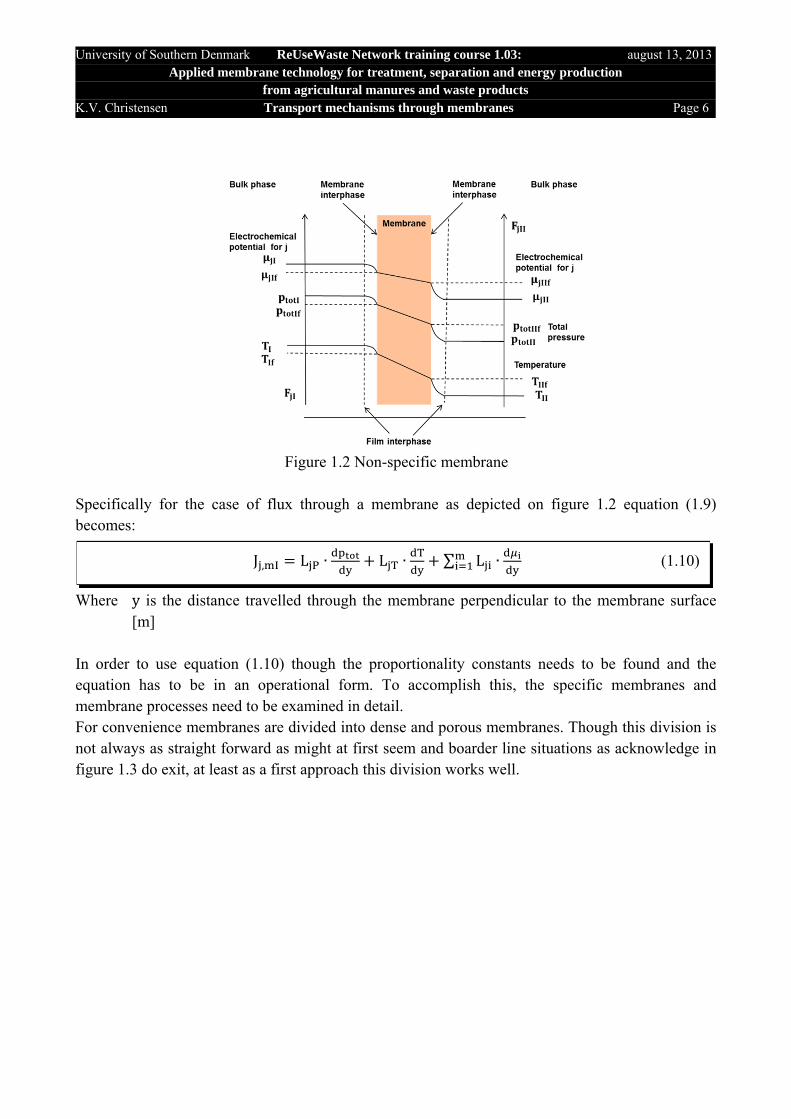
Figure 1.2 Non-specific membrane Specifically for the case of flux through a membrane as depicted on figure 1.2 equation (1.9) becomes:
Where y is the distance travelled through the membrane perpendicular to the membrane surface [m]
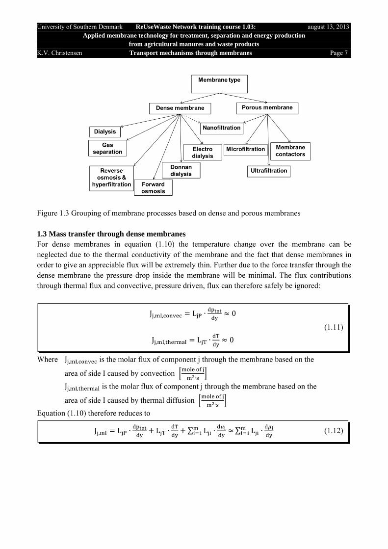
In order to use equation (1.10) though the proportionality constants needs to be found and the equation has to be in an operational form. To accomplish this, the specific membranes and membrane processes need to be examined in detail. For convenience membranes are divided into dense and porous membranes. Though this division is not always as straight forward as might at first seem and boarder line situations as acknowledge in figure 1.3 do exit, at least as a first approach this division works well.
J , L ∙ L ∙ ∑ L ∙ (1.10)
University of Southern Denmark ReUseWaste Network training course 1.03: august 13, 2013Applied membrane technology for treatment, separation and energy production
from agricultural manures and waste products K.V. Christensen Transport mechanisms through membranes Page 7
Figure 1.3 Grouping of membrane processes based on dense and porous membranes 1.3 Mass transfer through dense membranes For dense membranes in equation (1.10) the temperature change over the membrane can be neglected due to the thermal conductivity of the membrane and the fact that dense membranes in order to give an appreciable flux will be extremely thin. Further due to the force transfer through the dense membrane the pressure drop inside the membrane will be minimal. The flux contributions through thermal flux and convective, pressure driven, flux can therefore safely be ignored:
Where J , , is the molar flux of component j through the membrane based on the
area of side I caused by convection
∙
J , , is the molar flux of component j through the membrane based on the
area of side I caused by thermal diffusion
∙
Equation (1.10) therefore reduces to
J , , L ∙ 0
(1.11)
J , , L ∙ 0
J , L ∙ L ∙ ∑ L ∙ ∑ L ∙ (1.12)

University of Southern Denmark ReUseWaste Network training course 1.03: august 13, 2013Applied membrane technology for treatment, separation and energy production
from agricultural manures and waste products K.V. Christensen Transport mechanisms through membranes Page 8
If the expression for the electrochemical potential is inserted into (1.12) the flux equation simplifies to
Equation (1.13) can only be simplified further, by looking at specific membrane operations. 1.3.1 Dialysis Though dialysis is not used in biowaste treatment it is one of the most used membrane processes based on number of membrane modules produced each year and serves as a relatively simple process that illustrates some of the complexity when describing membrane fluxes. In dialysis a component j moves from a chamber with high concentration of j through a dense membrane to a chamber with a low concentration of j, as illustrated on figure 1.4. Figure 1.4 Transport during membrane dialysis. 1.3.1.1 Dialysis with membrane-solute interaction only As a first approach, the membrane is assumed so dense, that only the membrane material m and the component j interact inside the membrane. This assumption reduce the complexity of equation (1.13) to
Where m stands for the membrane
J , ∑ L ∙
⇓ (1.13)
J , ∑ L ∙∙ ∙ ∙ ∙ ∑ L ∙ R ∙ T ∙ z ∙ ∙
J , ∑ L ∙ R ∙ T ∙ z ∙ ∙
⇓ (1.14)
J , L ∙ R ∙ T ∙ z ∙ ∙ L ∙ R ∙ T ∙ z ∙ ∙
University of Southern Denmark ReUseWaste Network training course 1.03: august 13, 2013Applied membrane technology for treatment, separation and energy production
from agricultural manures and waste products K.V. Christensen Transport mechanisms through membranes Page 9
In dialysis no electrical field is applied across the membrane. Therefore equation (1.14) can be written as
The activity of the membrane though a solid may not actually be 1 as swollen membranes do interact with the liquid dissolved in the membrane, but the activity will not change appreciably with the distance y. Therefore only the change in activity of j is of concern. The activity of j can be expressed based on the fugacity:
Where f is the fugacity of j in the mixture Pa
f is the fugacity of j in its standard state Pa
The fugacity of a liquid mixture is given by
Where f is the fugacity of pure j Pa
x is the molecular fraction of j in the mixture
γ is the activity coefficient j in the mixture
Based on (1.16) and (1.17) the change in activity of component j can be expressed as
J , L ∙ R ∙ T ∙ z ∙ ∙ L ∙ R ∙ T ∙ z ∙ ∙
⇓ 0 (1.15)
J , L ∙ R ∙ T ∙ L ∙ R ∙ T ∙
a (1.16)
f γ ∙ x ∙ f (1.17)
lna ln∙ ∙
ln γ ∙ x ln
⇓ ∙
(1.18)
⇓ 0
∙
University of Southern Denmark ReUseWaste Network training course 1.03: august 13, 2013Applied membrane technology for treatment, separation and energy production
from agricultural manures and waste products K.V. Christensen Transport mechanisms through membranes Page 10
From the definition of fugacity the change in fugacity can be expressed as [1]:
Where V is the molecular volume of pure j
The expression for the change in activity therefore is
and the flux expression becomes
As the pressure change inside dense membranes is small (1.21) reduces to
For a dense membrane where there is only interaction between the membrane and the solute j even though the activity coefficient γj is not 1 and expectedly different from the activity coefficient of j in the solution outside the membrane, it can without much loss of accuracy be assumed, that γj inside the membrane does not change much with position in the direction y. Therefore the flux equation (1.21) can be simplified further to
dlnf∙dp (1.19)
∙
∙ (1.20)
J , L ∙ R ∙ T ∙ L ∙ R ∙ T ∙
⇓ 0
J , L ∙ R ∙ T ∙ (1.21)
⇓
J , L ∙ R ∙ T ∙∙
L ∙ V ∙
J , L ∙ R ∙ T ∙∙
L ∙ V ∙
⇓ 0 (1.22)
J , L ∙ R ∙ T ∙∙
L ∙ R ∙ T ∙
J , L ∙ R ∙ T ∙
⇓ 0 (1.23)
J , L ∙ R ∙ T ∙ L ∙ ∙ ∙

University of Southern Denmark ReUseWaste Network training course 1.03: august 13, 2013Applied membrane technology for treatment, separation and energy production
from agricultural manures and waste products K.V. Christensen Transport mechanisms through membranes Page 11
As the concentration in general can be expressed as
Where C is the molar concentration of j
C is the total molar concentration of j
this makes it possible to link the proportionality constant Ljj to the Fick’s law diffusivity coefficient of component j in the membrane, Dm,j:
Where D , is the diffusion coefficient for j relative to the membrane
The expression for Ljj is general and flux equation (1.14) for a solute which only interact with the dense membrane can therefore in general be stated as
To arrive at a flux equation for the simplified dialysis situation the flux equation (1.25) can be solved as an ordinary differential equation (ODE).
C x ∙ C (1.24)
J , L ∙ ∙ ∙ L ∙ ∙ ∙
∙∙
⇓ 0
J , L ∙ ∙
∙∙
∙L ∙ ∙ ∙
Fick slaw:J , D , ∙ (1.25)
⇓
L , ∙
∙
J , L ∙ R ∙ T ∙ z ∙ ∙
⇓ (1.26)
J , D , ∙ C ∙∙
∙
∙∙
University of Southern Denmark ReUseWaste Network training course 1.03: august 13, 2013Applied membrane technology for treatment, separation and energy production
from agricultural manures and waste products K.V. Christensen Transport mechanisms through membranes Page 12
If the membrane area is assumed independent of y the ODE can be solved easily by separation of the variables:
Where C , is the concentration of j inside membrane at position y = 0 (fig. 1.4)
C , is the concentration of j inside membrane at position y = ℓ (fig. 1.4)
ℓisthethicknessofthemembrane m Note that solving the first order ODE requires two boundary conditions as the flux, not the concentration, is assumed unknown. The concentration of component j inside the membrane is of cause normally unknown. It is the concentrations of j, CjI and CjII in the bulk fluid phase away from the membrane that are known. If CjI and CjII are known the concentrations in the fluid just outside the membrane, CjIf and CjIIf can also be determined. What is needed is therefore a connection between CjIf and CjIM and CjIIf and CjIIM. The classical approach is to assume equilibrium between the concentrations just ouside and inside the membrane:
Where C , is the concentration of j outside membrane at position y = 0 (fig. 1.4)
C , is the concentration of j outside membrane at position y = ℓ (fig. 1.4)
K , is distribution coefficient of concentration of j at position y = 0
K , is distribution coefficient of concentration of j at position y = ℓ
J , D , ∙
⇓
,
,
Boundarycondition:C C , aty 0C C , aty ℓ
⇓ (1.27)
dC,
,
,
,dy
ℓ ,
,∙ dy
ℓ
⇓
C , C ,,
,∙ ℓ
⇓
J ,,
ℓ∙ C , C ,
C , K , ∙ C , at y 0 (1.28)
C , K , ∙ C , at y ℓ
University of Southern Denmark ReUseWaste Network training course 1.03: august 13, 2013Applied membrane technology for treatment, separation and energy production
from agricultural manures and waste products K.V. Christensen Transport mechanisms through membranes Page 13
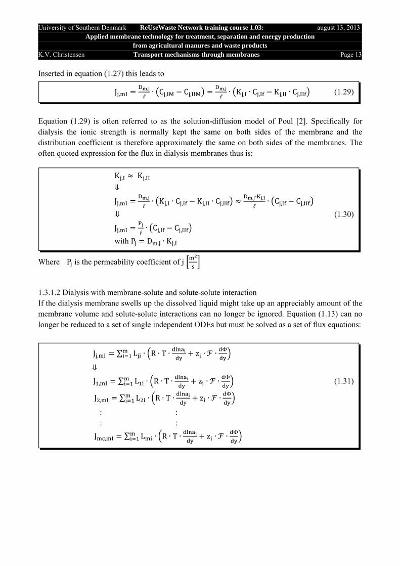
Inserted in equation (1.27) this leads to
Equation (1.29) is often referred to as the solution-diffusion model of Poul [2]. Specifically for dialysis the ionic strength is normally kept the same on both sides of the membrane and the distribution coefficient is therefore approximately the same on both sides of the membranes. The often quoted expression for the flux in dialysis membranes thus is:
Where P is the permeability coefficient of j
1.3.1.2 Dialysis with membrane-solute and solute-solute interaction If the dialysis membrane swells up the dissolved liquid might take up an appreciably amount of the membrane volume and solute-solute interactions can no longer be ignored. Equation (1.13) can no longer be reduced to a set of single independent ODEs but must be solved as a set of flux equations:
J ,,
ℓ∙ C , C ,
,
ℓ∙ K , ∙ C , K , ∙ C , (1.29)
K , K ,
⇓
J ,,
ℓ∙ K , ∙ C , K , ∙ C ,
, ∙ ,
ℓ∙ C , C ,
⇓ (1.30)
J , ℓ∙ C , C ,
with P D , ∙ K ,
J , ∑ L ∙ R ∙ T ∙ z ∙ ∙
⇓
J , ∑ L ∙ R ∙ T ∙ z ∙ ∙ (1.31)
J , ∑ L ∙ R ∙ T ∙ z ∙ ∙
: : : :
J , ∑ L ∙ R ∙ T ∙ z ∙ ∙

University of Southern Denmark ReUseWaste Network training course 1.03: august 13, 2013Applied membrane technology for treatment, separation and energy production
from agricultural manures and waste products K.V. Christensen Transport mechanisms through membranes Page 14
or in matrix form:
where is a a vector of dimension m containing the individual derivatives of lnai as
defined by equation (1.33) J is a vector of the dimension mc containing the individual flux values
L is an mc x mc matrix containing the individual proportionality constants as defined
by equation (1.34) Z is a diagonal mc x mc matrix containing the individual molecular charges as seen in
equation (1.35) The activity driving force vector is
while the proportionality matrix is given by
and the diagonal charge matrix is
J R ∙ T ∙ L ∙ ∙ L ∙ Z ∙ (1.32)
::
(1.33)
L
L L ⋯L L ⋯⋯ ⋯ ⋯
⋯ ⋯ L⋯ ⋯ L⋯ ⋯ ⋯
⋯ ⋯ ⋯⋯ ⋯ ⋯L L ⋯
⋯ ⋯ ⋯⋯ ⋯ ⋯⋯ ⋯ L
(1.34)
Z
z 0 00 z 00 0 z
⋯ ⋯ 0⋯ ⋯ 0⋯ ⋯ ⋯
⋯ ⋯ ⋯⋯ ⋯ ⋯0 0 0
⋯ ⋯ ⋯⋯ ⋯ ⋯⋯ ⋯ z
(1.35)

University of Southern Denmark ReUseWaste Network training course 1.03: august 13, 2013Applied membrane technology for treatment, separation and energy production
from agricultural manures and waste products K.V. Christensen Transport mechanisms through membranes Page 15
For dialysis no electrical field is applied. Further, at least as a first approximation, it can be assumed that the activity coefficient is nearly independent of the position inside the membrane. Therefore equation (1.32) simplifies to
where is a vector of dimension m containing the individual derivatives of xi
x is a diagonal matrix holding the molecular fractions xi in its diagonal
In order to get an expression for the values of the proportionality constants the Stefan-Maxwell description for multicomponent diffusion is used:
where D , is the binary diffusion coefficient for component i and j inside the membrane
m is the total number of components present inside the membrane including the membrane The Stefan-Maxwell equation implicitly assumes that the sum of fluxes of all components is zero, or in other words the fluxes are relative to either the total velocity of the system or to a reference component. In the case of dense membranes a logical choice is to calculate the fluxes of the fluid components relative to the flux of the membrane and thus include the membrane as one of the system components, m. This leads to:
where D , is the binary diffusion coefficient for component i and j inside the membrane
mc is the total number of components present inside the membrane excluding the membrane
J R ∙ T ∙ L ∙ R ∙ T ∙ L ∙ R ∙ T ∙ L ∙ x ∙ (1.36)
∑∙ , ∙ ,
∙ , (1.37)
0 ∑ J , ⇒ J , ∑ J , J , ∑ J , (1.39)

University of Southern Denmark ReUseWaste Network training course 1.03: august 13, 2013Applied membrane technology for treatment, separation and energy production
from agricultural manures and waste products K.V. Christensen Transport mechanisms through membranes Page 16
Equation (1.37) now yields
where β is a phenomenalogical constant which for purely molecular diffusivity is defined by
equation (1.39) For purely molecular diffusive transport the phenomenological constants are defined from:
Equation (1.39) can now be stated as a set of coupled ODEs:
Comparing equation (1.41) with equation (1.36) yields values for L:
If the change in activity coefficients through the membrane is assumed negligible the flux can be found by solving the coupled ODEs of equation (1.41) with the boundary conditions shown in (1.43) and treating the fluxes as the true unknowns.
⇓
C ∙ ∑∙ , ∙ ,
∙ ,J , ∙ ∑
,x ∙ ∑ ,
,x ∙ ,
,
⇓
C ∙ J , ∙ ∑, ,
x ∙ ∑, ,
∙ J , (1.39)
C ∙ β , ∙ J , ∑ β , ∙ J ,
β , ∑, ,
(1.40)
β ,, ,
∙ x for i j
∙ β ∙ J (1.41)
L∙∙ x ∙ β (1.42)
∙ β ∙ J (1.43)
Boundarycondition:C C , K , ∙ C , at y 0C C , K , ∙ C , at y ℓ
University of Southern Denmark ReUseWaste Network training course 1.03: august 13, 2013Applied membrane technology for treatment, separation and energy production
from agricultural manures and waste products K.V. Christensen Transport mechanisms through membranes Page 17
This procedure is of cause iterative, but should not be unduly complex, if the diffusion coefficients are to be found. This seldom is the case and the diffusion coefficients will have to be determined from laboratory experiments. If the influence of the activity coefficients have to be included, since L is now known, these effects
can be included easily. As the activity coefficient is a function of temperature, pressure and molecular fraction only and as pressure and temperature is constant inside the membrane, the activity coefficient’s dependence on position can be expressed as
Inserted into the flux equation (1.31) this leads to:
or in matrix form:
where La is an mc x mc matrix containing the individual proportionality constants as defined
by equation (1.47)
γ γ T, p , x
⇓ 0, 0, (1.44)
∙ ∙ ∑ ∙
J , ∑ L ∙ R ∙ T ∙ z ∙ ∙
⇓
J , R ∙ T ∙ ∑ L ∙ ∙ ∙
⇓
J , R ∙ T ∙ ∑ L ∙ ∙ ∙ ∑ ∙
⇓
J , R ∙ T ∙ ∑ L ∙ ∙ ∑ L ∙ ∙ ∑ ∙ (1.45)
⇓
J , R ∙ T ∙ ∑ L ∙ ∙ ∑ ∑ L ∙ ∙ ∙
⇓
J , R ∙ T ∙ ∑ L ∙ ∙ ∑ ∑ L ∙ ∙ ∙
⇓
J , R ∙ T ∙ ∑ L ∙ ∑ L ∙ ∙ ∙
J R ∙ T ∙ La ∙ (1.46)
University of Southern Denmark ReUseWaste Network training course 1.03: august 13, 2013Applied membrane technology for treatment, separation and energy production
from agricultural manures and waste products K.V. Christensen Transport mechanisms through membranes Page 18
The individual entries to the La matrix are found from (1.45) to be:
Equation (1.47) can now be stated as a set of coupled ODEs:
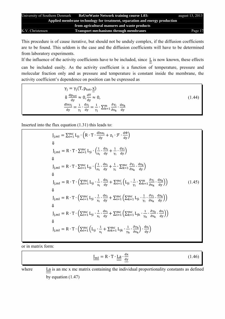
Again finding the fluxes from (1.48) is of cause iterative. The approach used for dialysis can with some modifications be used for other dense membrane separation processes. 1.3.2 Reverse osmosis (RO) Reverse osmosis is the classical method for separating ions like potassium and sodium from water producing a salt concentrate and potable water. It is thus of interest in biowaste treatment as it can be used as an end of the line process making water recycle possible and producing a fraction rich in potassium. Further reverse osmosis has a possibility as a process for separating ammonia from ionic solutions, which might become of interest in the future. In reverse osmosis the fact that the chemical potential is influenced by pressure is used as the driving force, making a component j move from a chamber at high pressure but low concentration of j through a dense membrane to a chamber with at a lower total pressure but with a higher concentration of j, as illustrated on figure 1.5.
Figure 1.5 Transport during reverse osmosis.
La L ∙ ∑ L ∙ ∙ (1.47)
∙∙ La ∙ J (1.48)
Boundarycondition:C C , K , ∙ C , at y 0C C , K , ∙ C , at y ℓ

University of Southern Denmark ReUseWaste Network training course 1.03: august 13, 2013Applied membrane technology for treatment, separation and energy production
from agricultural manures and waste products K.V. Christensen Transport mechanisms through membranes Page 19
1.3.2.1 Reverse osmosis with membrane-solute interaction only As a first approach, the membrane is assumed so dense, that only the membrane material m and the component j interact inside the membrane. Further the pressure drop and temperature change inside the membrane is assumed negligible. The transport through the membrane therefore happens by diffusion just as for dialysis and equation (1.27) is thus still valid. Again the relation between the concentration outside the membrane and inside the membrane can be expressed by equation
Again the relation between the concentration outside the membrane and inside the membrane can be expressed by equation (1.28):
And therefore equation (1.29) is also valid as a solution for the flux through the RO membrane:
But as the pressure difference between side I and side II is large K , K , and equation (1.30) is
thus not valid for RO.
,
,
Boundarycondition:C C , aty 0C C , aty ℓ
⇓ (1.27)
J ,,
ℓ∙ C , C ,
C , K , ∙ C , at y 0 (1.28)
C , K , ∙ C , at y ℓ
J ,,
ℓ∙ C , C ,
,
ℓ∙ K , ∙ C , K , ∙ C , (1.29)

University of Southern Denmark ReUseWaste Network training course 1.03: august 13, 2013Applied membrane technology for treatment, separation and energy production
from agricultural manures and waste products K.V. Christensen Transport mechanisms through membranes Page 20
To simplify the flux equation (1.30) further it is assumed that equilibrium between the membrane and the liquid phase is attained at the membrane-liquid interphase. In thermodynamic terms this leads to
Where a , is the activity of component j in the mixture outside the membrane at interface II
a , is the activity of component j in the membrane at interface II
Φ is the electrical potential in the mixture outside the membrane at interface II V Φ is the electrical potential in the mixture in the membrane at interface II V , is the chemical potential of component j in the mixture outside the membrane at
interface II
, is the chemical potential of component j in the membrane at interface II
Since the temperature is assumed constant and no electrical potential difference is involved this leads to:
Where C , is the total concentration in the membrane
p , is the pressure in chamber I [Pa]
p , is the pressure in chamber II [Pa]
p , is the pressure in the mixture outside the membrane at interface II [Pa]
p , is the pressure in the membrane at interface II [Pa]
γ , is the activity coefficient of j in the membrane at interface I
γ , is the activity coefficient of j in the mixture outside the membrane at interface II
γ , is the activity coefficient of j in the membrane at interface II
, ,
⇓ (1.49) R ∙ T ∙ lna , z ∙ ∙ Φ , R ∙ T ∙ lna , z ∙ ∙ Φ
lna , lna ,
⇓
ln γ , ∙ x , ∙∙ p , ln γ , ∙ x , ∙
∙ p ,
⇓
x , x , ∙ ,
,∙ exp
∙ , ,
∙
⇓ (1.50)
C , C , ∙ ,
,∙ ,
,∙ exp
∙ , ,
∙
⇓ γ , γ , , p , p , p , , p , p , , C , C ,
C , C , ∙ ,
,∙ ,
,∙ exp
∙ , ,
∙

University of Southern Denmark ReUseWaste Network training course 1.03: august 13, 2013Applied membrane technology for treatment, separation and energy production
from agricultural manures and waste products K.V. Christensen Transport mechanisms through membranes Page 21
If furthermore the difference in activity coefficient between system I and system II is small:
Where γ , is the activity coefficient of j in the mixture outside the membrane at interface II
equations (1.50) and (1.51) leads to
and therefore
Equation (1.53) applies for both solvent, usually water, and solute, usually a form of salt. It can though be transformed into a more classical form if the difference in concentrations Cj,If and CjIIf is expressed by the osmotic pressure difference. At equilibrium equation (1.54) becomes
where J , , is the flux of j through the membrane at equilibrium
∙
p , , is the pressure in chamber I at equilibrium [Pa]
p , , is the pressure in chamber II at equilibrium [Pa]
∆ is the osmotic pressure difference between camber I and II [Pa] Inserted into equation (1.54) this yields
,
,∙ ,
,
,
,∙ ,
,
,
,K , (1.51)
C , C , ∙ K , ∙ exp∙ , ,
∙ (1.52)
J ,,
ℓ∙ K , ∙ C , K , ∙ C ,
, ∙ ,
ℓ∙ C , C , ∙ exp
∙ , ,
∙ (1.53)
J , , 0 , ∙ ,
ℓ∙ C , C , ∙ exp
∙ , , , ,
∙
⇓ (1.54)
C , C , ∙ exp∙ , , , ,
∙C , ∙ exp
∙∆
∙
J ,, ∙ , ∙ ,
ℓ∙ 1 exp
∙ , , ∆
∙ (1.55)

University of Southern Denmark ReUseWaste Network training course 1.03: august 13, 2013Applied membrane technology for treatment, separation and energy production
from agricultural manures and waste products K.V. Christensen Transport mechanisms through membranes Page 22
Equation (1.55) works for both solvent, usually water, and solute, typically salts, but if one first look at the solvent (1.55) can be simplified further close to equilibrium:
and equation (1.55) becomes
where A is the solvent permeability constant defined by equation (1.58)
∙ ∙
∆P is the pressure difference between chamber I and II [Pa] The solvent permeability Aj is defined by
but is normally found from experiments. For the solute equation (1.53) is often simplified directly to
where B is the solute permeability constant defined by equation (1.60)
The solute permeability Bj is defined by
but is normally found from experiments.
J ,, ∙ , ∙ , ∙
ℓ∙ ∙∙ p , p , ∆ A ∙ ∆P ∆π (1.57)
A , ∙ , ∙ , ∙
ℓ∙ ∙ (1.58)
J ,, ∙ ,
ℓ∙ C , C , ∙ exp
∙ , ,
∙
⇓ exp∙ , ,
∙1
J ,, ∙ ,
ℓ∙ C , C , (1.59)
⇓
J , B ∙ C , C ,
B , ∙ ,
ℓ (1.60)
lim∙ , , ∆
∙→ 0
⇓
lim 1 exp∙ , , ∆
∙→ 1 1
∙ , , ∆
∙ (1.56)
⇓
lim 1 exp∙ , , ∆
∙→
∙ , , ∆
∙
University of Southern Denmark ReUseWaste Network training course 1.03: august 13, 2013Applied membrane technology for treatment, separation and energy production
from agricultural manures and waste products K.V. Christensen Transport mechanisms through membranes Page 23
1.3.2.2 RO with membrane-solute and solute-solute interaction In high flux RO the membrane swells up and dissolved liquid might take up an appreciably amount of the membrane volume and solute-solute interactions can no longer be ignored. If the influence of the activity coefficient gradient inside the membrane is ignored, equation (1.43) still holds:
If the activity coefficient gradient is to be included, equation (1.48) should be used:
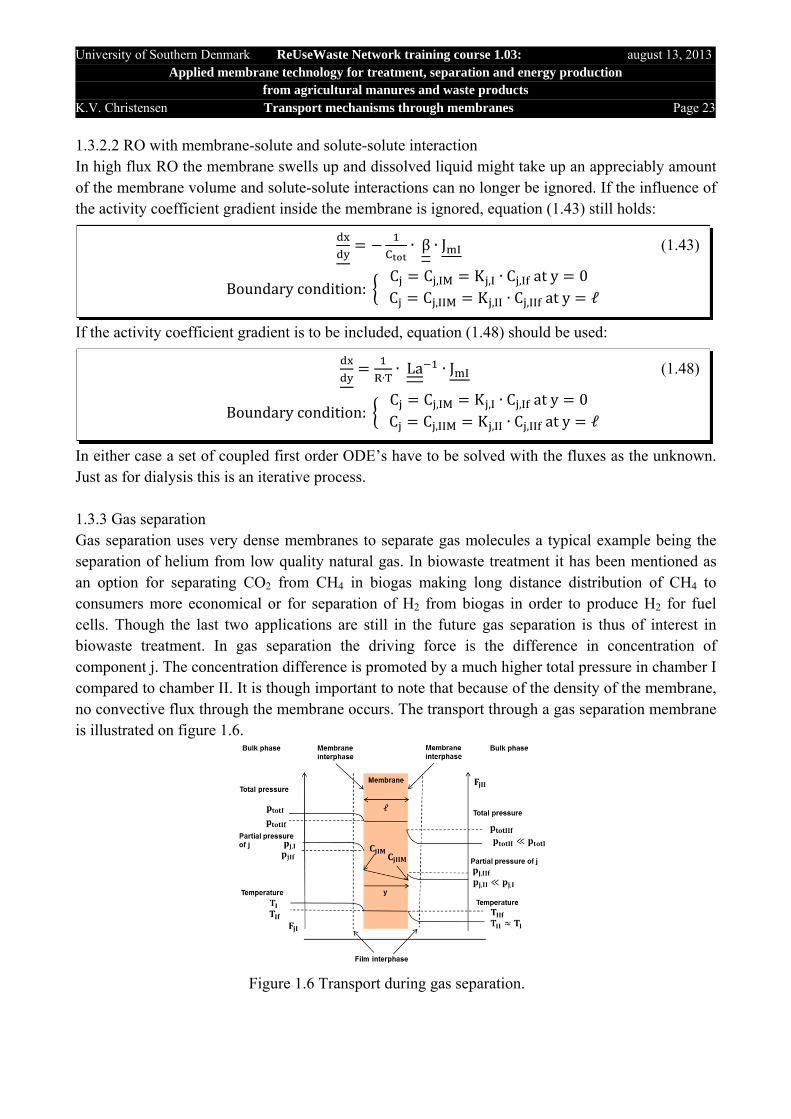
In either case a set of coupled first order ODE’s have to be solved with the fluxes as the unknown. Just as for dialysis this is an iterative process. 1.3.3 Gas separation Gas separation uses very dense membranes to separate gas molecules a typical example being the separation of helium from low quality natural gas. In biowaste treatment it has been mentioned as an option for separating CO2 from CH4 in biogas making long distance distribution of CH4 to consumers more economical or for separation of H2 from biogas in order to produce H2 for fuel cells. Though the last two applications are still in the future gas separation is thus of interest in biowaste treatment. In gas separation the driving force is the difference in concentration of component j. The concentration difference is promoted by a much higher total pressure in chamber I compared to chamber II. It is though important to note that because of the density of the membrane, no convective flux through the membrane occurs. The transport through a gas separation membrane is illustrated on figure 1.6. Figure 1.6 Transport during gas separation.
∙ β ∙ J (1.43)
Boundarycondition:C C , K , ∙ C , at y 0C C , K , ∙ C , at y ℓ
∙∙ La ∙ J (1.48)
Boundarycondition:C C , K , ∙ C , at y 0C C , K , ∙ C , at y ℓ

University of Southern Denmark ReUseWaste Network training course 1.03: august 13, 2013Applied membrane technology for treatment, separation and energy production
from agricultural manures and waste products K.V. Christensen Transport mechanisms through membranes Page 24
1.3.3.1 Gas separation with membrane-solute interaction only In most gas separation membranes the membrane is so dense, that only the membrane material m and the component j interact inside the membrane. Further the pressure drop and temperature change inside the membrane is assumed negligible. The transport through the membrane therefore happens by diffusion just as for dialysis and equation (1.27) is thus still valid. Again the relation between the concentration outside the membrane and inside the membrane can be expressed by equation
Again the relation between the concentration outside the membrane and inside the membrane can be expressed by equation (1.28):
And therefore equation (1.29) is also valid as a solution for the flux through the gas separation membrane:
But as the pressure difference between side I and side II is large K , K , and equation (1.30) is
thus not generally valid for gas separation. To simplify the flux equation (1.29) further it is assumed that equilibrium between the membrane and the gas phase is attained at the membrane-liquid interphase. Since the temperature is assumed constant and no electrical potential difference is involved, just as for RO in thermodynamic terms this leads to
,
,
Boundarycondition:C C , aty 0C C , aty ℓ
⇓ (1.27)
J ,,
ℓ∙ C , C ,
C , K , ∙ C , at y 0 (1.28)
C , K , ∙ C , at y ℓ
J ,,
ℓ∙ C , C ,
,
ℓ∙ K , ∙ C , K , ∙ C , (1.29)
lna , lna ,
⇓ (1.61) a , a ,
University of Southern Denmark ReUseWaste Network training course 1.03: august 13, 2013Applied membrane technology for treatment, separation and energy production
from agricultural manures and waste products K.V. Christensen Transport mechanisms through membranes Page 25
Since the components in chamber I and II are all gases the activities are more properly expressed as functions of their fugacities:
Where f , is the fugacity of component j in the mixture outside the membrane at interface II [Pa]
f , is the fugacity of component j in the mixture in the membrane at interface II [Pa]
The fugacity in the gas phase can be expressed as function of its fugacity coefficient [1] leading to:
Where p is vapor pressure of pure j at the process temperature [Pa]
φ is fugacity coefficient of pure j at the process temperature and pressure
φ , is the fugacity coefficient of j in the mixture outside the membrane at interface II
Equation (1.63) can then be used to derive a relation between the concentration of j in the gas phase and the concentration of j dissolved in the membrane:
For gas separation the distribution factor on side II therefore is:
a , a ,
⇓
, , (1.62)
⇓
f , f ,
K ,, ∙ ,
, ∙ ∙∙ exp
∙ ,
∙ (1.64)
x , ∙ γ , ∙ p ∙ φ ∙ exp∙ ,
∙x , ∙ φ , ∙ p ,
⇓ (1.63)
C , x , ∙ C ,, ∙ ,
, ∙ ∙∙ exp
∙ ,
∙∙ x , ∙ p ,
⇓ C , K , ∙ x , ∙ p , K , ∙ x , ∙ p ,
f , f ,
⇓ (1.63)
x , ∙ γ , ∙ p ∙ φ ∙ exp∙ ,
∙x , ∙ φ , ∙ p ,
University of Southern Denmark ReUseWaste Network training course 1.03: august 13, 2013Applied membrane technology for treatment, separation and energy production
from agricultural manures and waste products K.V. Christensen Transport mechanisms through membranes Page 26
A similar equation can be derived for the distribution factor on side I s:
Where φ , is the fugacity coefficient of j in the mixture outside the membrane at interface I
As the activity coefficients, the total pressure and the total concentration often do not change appreciably inside the membrane and the fugacity coefficients in the gas phase often are close to 1, Kj,II can be expressed by KjI:
and therefore
where p , is the partial pressure of j in the mixture outside the membrane at interface I [Pa]
p , is the partial pressure of j in the mixture outside the membrane at interface II [Pa]
1.3.2.2 Gas separation with membrane-solute and solute-solute interaction In most present industrial applications solute-solute interaction inside the membrane volume is not considered to have appreciable influence on the flux. If solute-solute interactions cannot be ignored equation (1.43) is still valid, if the influence of the activity coefficient gradient inside the membrane can be ignored:
J ,,
ℓ∙ K , ∙ p , K , ∙ p ,
, ∙ ,
ℓ∙ p , p , (1.67)
∙ β ∙ J (1.43)
Boundarycondition:C C , K , ∙ p , at y 0C C , K , ∙ p , at y ℓ
K ,, ∙ ,
, ∙ ∙∙ exp
∙ ,
∙ (1.65)
K ,, ∙ ,
, ∙ ∙∙ exp
∙ ,
∙
⇓ γ , γ , , φ , φ , , p , p , , C , C , (1.66)
K ,, ∙ ,
, ∙ ∙∙ exp
∙ ,
∙K ,

University of Southern Denmark ReUseWaste Network training course 1.03: august 13, 2013Applied membrane technology for treatment, separation and energy production
from agricultural manures and waste products K.V. Christensen Transport mechanisms through membranes Page 27
If the activity coefficient gradient is to be included, equation (1.48) should be used:
In either case a set of coupled first order ODE’s have to be solved with the fluxes as the unknown. Just as for dialysis this is an iterative process.
1.3.4 Pervaporation In pervaporation one or more volatile compounds are evaporated from a liquid phase through a membrane into a gas phase. The method has been investigated as a method to recover volatile aromatics from wastewater from cabbage processing plants but has as yet to be proven of interest in animal slurry treatment. A point of investigation could be selective removal of volatile fatty acids or ammonia. As for gas separation the driving force is the difference in concentration of component j. The concentration difference is promoted by creating a high vapor pressure in chamber I by increasing the temperature while at the same time keeping the total pressure low in chamber II by creating a vacuum. Even though the process is described by differences in partial pressures it should be made clear that because of the density of the membrane, no convective flux through the membrane occurs and that the actual evaporation happens at interphase II. The transport through a pervaporation membrane thus is a liquid phase diffusion as illustrated on figure 1.7.
Figure 1.7 Transport during pervaporation. 1.3.4.1 Pervaporation with membrane-solute interaction only In most pervaporation processes the membrane swells to an appreciably extent making the assumption that only membrane-solute interaction occurs less likely. None the less this is often
∙∙ La ∙ J (1.48)
Boundarycondition:C C , K , ∙ p , at y 0C C , K , ∙ p , at y ℓ

University of Southern Denmark ReUseWaste Network training course 1.03: august 13, 2013Applied membrane technology for treatment, separation and energy production
from agricultural manures and waste products K.V. Christensen Transport mechanisms through membranes Page 28
assumed and it forms a simple background for deriving some of the basic relations between the membrane and the liquid and gas at the interphases I and II respectively. Further the pressure drop and temperature change inside the membrane is assumed negligible. The transport through the membrane therefore happens by diffusion just as for dialysis and equation (1.27) is thus still valid:
Again the relation between the concentration outside the membrane and inside the membrane can be expressed by equation (1.28):
And therefore equation (1.29) is also valid as a solution for the flux through the gas separation membrane:
To simplify the flux equation (1.29) further it is assumed that equilibrium between the membrane and the liquid phase is attained at the membrane-liquid interphase. On side II the process is identical to the situation for gas separation and KjII can therefore be expressed by equation (1.64):
On side I it is actually a liquid that is in equilibrium with the membrane at interphase I, but to in order to express (1.29) as a function of partial pressures the following approach is used.
,
,
Boundarycondition:C C , aty 0C C , aty ℓ (1.27)
⇓
J ,,
ℓ∙ C , C ,
C , K , ∙ C , at y 0 (1.28)
C , K , ∙ C , at y ℓ
J ,,
ℓ∙ C , C ,
,
ℓ∙ K , ∙ C , K , ∙ C , (1.29)
K ,, ∙ ,
, ∙ ∙∙ exp
∙ ,
∙ (1.64)
University of Southern Denmark ReUseWaste Network training course 1.03: august 13, 2013Applied membrane technology for treatment, separation and energy production
from agricultural manures and waste products K.V. Christensen Transport mechanisms through membranes Page 29
First equilibrium between the liquid phase and membrane phase is assumed at interphase I. Next the activity of the liquid phase is expressed by the corresponding hypothetical equilibrium gas phase equation:
Where f , is the fugacity of component j in the gas phase at conditions outside the membrane at
interface II [Pa]
f , ℓ is the fugacity of component j in the liquid phase at conditions outside the membrane
at interface II [Pa]
The fugacities in the gas phase can be expressed as function of its fugacity coefficient [1] and the fugacities in the liquid and membrane based on activities leads to:
Where γ , ℓ is the activity coefficient of component j in the liquid phase at conditions outside the
membrane at interface I φ , is the fugacity coefficient of component j in the gas phase at conditions outside the
membrane at interface I φ , ℓ is the fugacity coefficient of component j in the liquid phase at conditions outside the
membrane at interface I
a , a , ℓ a ,
⇓
, , ℓ , (1.68)
⇓
f , f , ℓ f ,
⇓
⇓
f , f , ℓ
x , ∙ φ , ∙ p , x , ℓ ∙ γ , ℓ ∙ p ∙ φ ∙ exp∙ ,
∙
f , ℓ f ,
⇓ (1.69)
x , ℓ ∙ γ , ℓ ∙ p ∙ φ ∙ exp∙ ,
∙x , ∙ γ , ∙ p ∙ φ ∙ exp
∙ ,
∙
⇓
f , f ,
x , ∙ φ , ∙ p , x , ∙ γ , ∙ p ∙ φ ∙ exp∙ ,
∙
University of Southern Denmark ReUseWaste Network training course 1.03: august 13, 2013Applied membrane technology for treatment, separation and energy production
from agricultural manures and waste products K.V. Christensen Transport mechanisms through membranes Page 30
For side I, a distribution coefficient based on the partial pressures exerted by the liquid phase can therefore be expressed as:
and the distribution factor on side I therefore is:
As the activity coefficients, the total pressure and the total concentration often do not change appreciably inside the membrane and the fugacity coefficients in the gas phase often are close to 1, Kj,II can be expressed by KjI:
and therefore
It looks similar to gas separation but it has to be remembered that the partial pressure of j in chamber I has to be calculated from:
K ,, ∙ ,
, ∙ ∙∙ exp
∙ ,
∙ (1.71)
J ,,
ℓ∙ K , ∙ p , K , ∙ p ,
, ∙ ,
ℓ∙ p , p , (1.73)
x , ∙ φ , ∙ p , x , ∙ γ , ∙ p ∙ φ ∙ exp∙ ,
∙
⇓ (1.70)
C , x , ∙ C ,, ∙ ,
, ∙ ∙∙ exp
∙ ,
∙∙ x , ∙ p ,
⇓ C , K , ∙ x , ∙ p ,
K ,, ∙ ,
, ∙ ∙∙ exp
∙ ,
∙
⇓ γ , γ , , φ , φ , , p , p , , C , C , (1.72)
K ,, ∙ ,
, ∙ ∙∙ exp
∙ ,
∙K ,
x , ∙ φ , ∙ p , x , ∙ γ , ∙ p ∙ φ ∙ exp∙ ,
∙
⇓ φ , 1, φ 1, p , low to moderate (1.74)
x , ∙ p , p , x , ∙ γ , ∙ p

University of Southern Denmark ReUseWaste Network training course 1.03: august 13, 2013Applied membrane technology for treatment, separation and energy production
from agricultural manures and waste products K.V. Christensen Transport mechanisms through membranes Page 31
So the influence of increase the total pressure will be small compared to increasing the temperature in pervaporation. 1.3.4.2 Pervaporation with membrane-solute and solute-solute interaction For most industrial applications solute-solute interaction inside the membrane volume should be considered when describing pervaporation, as most membranes swell appreciably during the process. If the if the influence of the activity coefficient gradient inside the membrane can be ignored equation (1.43) is still valid:
Though the activity coeffients may change appreciably inside the membrane equation (1.43) often have to do, as information on activity coeffcients inside membranes are limited. If the activity coefficient gradient is to be included, equation (1.48) should be used:
As for dialysis, reverse osmosis and gas separation solving these coupled first order ODE’s have to be solved with the fluxes as the unknowns by an iterative process.
∙ β ∙ J (1.43)
Boundarycondition:C C , K , ∙ p , at y 0C C , K , ∙ p , at y ℓ
∙∙ La ∙ J (1.48)
Boundarycondition:C C , K , ∙ p , at y 0C C , K , ∙ p , at y ℓ
University of Southern Denmark ReUseWaste Network training course 1.03: august 13, 2013Applied membrane technology for treatment, separation and energy production
from agricultural manures and waste products K.V. Christensen Transport mechanisms through membranes Page 32
1.4 Mass transfer through porous membranes For mass transfer through porous membranes equation (1.10) is still valid:
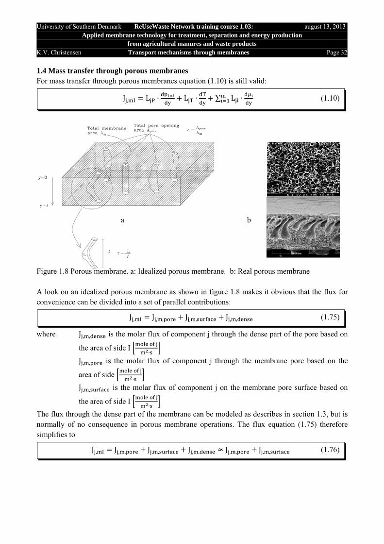
a b Figure 1.8 Porous membrane. a: Idealized porous membrane. b: Real porous membrane A look on an idealized porous membrane as shown in figure 1.8 makes it obvious that the flux for convenience can be divided into a set of parallel contributions:
where J , , is the molar flux of component j through the dense part of the pore based on
the area of side I
∙
J , , is the molar flux of component j through the membrane pore based on the
area of side
∙
J , , is the molar flux of component j on the membrane pore surface based on
the area of side I
∙
The flux through the dense part of the membrane can be modeled as describes in section 1.3, but is normally of no consequence in porous membrane operations. The flux equation (1.75) therefore simplifies to
J , L ∙ L ∙ ∑ L ∙ (1.10)
J , J , , J , , J , , (1.75)
J , J , , J , , J , , J , , J , , (1.76)
University of Southern Denmark ReUseWaste Network training course 1.03: august 13, 2013Applied membrane technology for treatment, separation and energy production
from agricultural manures and waste products K.V. Christensen Transport mechanisms through membranes Page 33
The flux through the porous part of the membrane can still be described by equation (1.10), but in this case the convective pressure driven part cannot in general be ignored and in a few, probably non-relevant cases, the thermal part cannot be ignored either. Therefore the porous flux is divided into three additive contributions:
where J , is the convective molar flux of component j through the porous part of the
membrane
∙
J , is the diffusive molar flux of component j through the porous part of the
membrane
∙
J , is the thermal molar flux of component j through the porous part of the
membrane
∙
1.4.1 Modeling the convective flux term in porous membranes In order to use equation (1.10) the proportionality constant LjP needs to be found. The flow inside the membrane pore will in general be laminar. For straight pores the Poseuille equation can therefore be used to describe the flow through the pore:
where r is the pore mean radius [m]
v is the velocity of the fluid
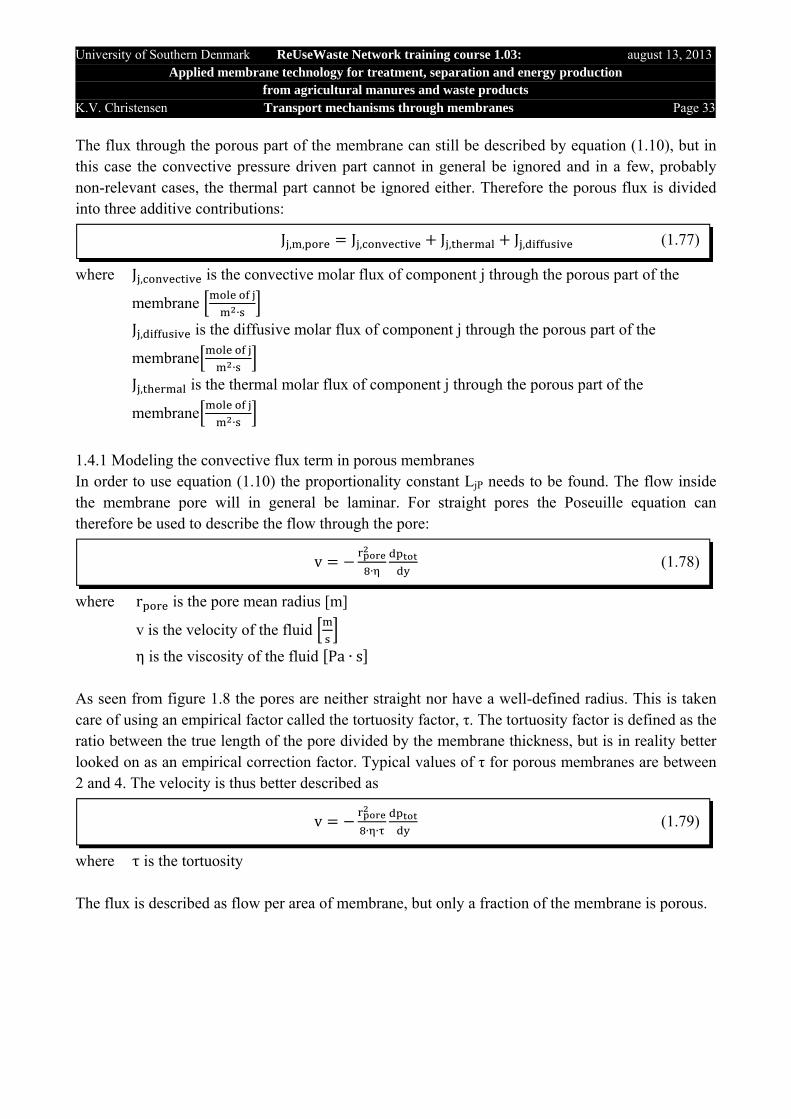
η is the viscosity of the fluid Pa ∙ s As seen from figure 1.8 the pores are neither straight nor have a well-defined radius. This is taken care of using an empirical factor called the tortuosity factor, τ. The tortuosity factor is defined as the ratio between the true length of the pore divided by the membrane thickness, but is in reality better looked on as an empirical correction factor. Typical values of τ for porous membranes are between 2 and 4. The velocity is thus better described as
where τ is the tortuosity The flux is described as flow per area of membrane, but only a fraction of the membrane is porous.
v∙
(1.78)
v∙ ∙
(1.79)
J , , J , J , J , (1.77)
University of Southern Denmark ReUseWaste Network training course 1.03: august 13, 2013Applied membrane technology for treatment, separation and energy production
from agricultural manures and waste products K.V. Christensen Transport mechanisms through membranes Page 34
This fraction can be determined experimentally as the membrane porosity ε. Based on this the convective flux through the membrane becomes:
where ε is the porosity of the membrane Equation (1.80) holds well for fairly cylindrical pores as obtained by membrane track etching or stretching. For membranes made by sintering smaller particle together, like ceramic membranes, the straight pore assumption does not apply. Instead the Kozeny-Carman description based on randomly packed spheres is used:
where K is a shape constant based on the sinter particles s is the internal surface area of the pore [m2] The convective flux in this case can be estimated as
The shape constant K and internal surface area s is seldom known. As a first estimate their influence can be estimated from
where dp is the diameter of the original sinter pellets from which the membrane was made [m] sf is the sphericity of the original sinter pellet from which the membrane was made In equation (1.83) the sphericity is calculated as
Summarizing the convective flux through the pore can be estimated using D’Arcy’s law (1.85) which is a generalization of the Poseuille and the Kozeny-Carman equations:
Where KD is the D’Arcy constants [m2]
J , C ∙ v C ∙∙
∙ ∙ (1.80)
v∙
∙ ∙ ∙ (1.81)
J , C ∙ v C ∙∙
∙ ∙ ∙ (1.82)
K ∙ s∙
(1.83)
sf ∙ (1.84)
J , C ∙ v C ∙ (1.85)

University of Southern Denmark ReUseWaste Network training course 1.03: august 13, 2013Applied membrane technology for treatment, separation and energy production
from agricultural manures and waste products K.V. Christensen Transport mechanisms through membranes Page 35
Where the constant KD can be estimated using either the Poseuille equation or the Kozeny-Carman equation, but is best considered an empirical constant specific to each membrane. The proportionality factor Lj,P therefore is
1.4.2 Modeling the thermal flux term in porous membranes For liquids the influence of thermal flux can be neglected. The same is true for low temperature applications. Only at very high temperatures, as in flames, will the thermal flux contribute to the total flux to an appreciable amount. For gases the thermal flux can be estimated from [3]:
Where D , is the thermal diffusivity ∙
The thermal diffusion coefficient can be estimated from [4]:
Where M , is the molecular weight of component j
The proportionality factor Lj,T therefore is
In most industrial membrane applications thermal diffusion is unimportant though it has been used for isotope separation in the past.
D’Arcy’s law: L , C ∙
Poseuille’s law: L , C ∙∙
∙ ∙ (1.86)
Kozeny-Carman equation: L , C ∙∙
∙ ∙ ∙
J , ∙ D , ∙ (1.87)
D , 2.59 ∙ 10 ∙ M , ∙ T . ∙ ,. ∙
∑ ,. ∙
, ∙
∑ , ∙∙
∑ ,. ∙
∑ ,. ∙
(1.88)
L , ∙ D , ∙ (1.89)
University of Southern Denmark ReUseWaste Network training course 1.03: august 13, 2013Applied membrane technology for treatment, separation and energy production
from agricultural manures and waste products K.V. Christensen Transport mechanisms through membranes Page 36
1.4.3 Modeling the diffusive flux term in porous membranes The convective flux term in the pore can be modeled based on the same principle as the convective flux in dense membranes except for the fact that the binary diffusion coefficient, Dij, for the gasses or liquids in the pores are not influenced by the presence of the membrane and that the fluid membrane interaction coefficient, Djm, is described by the Knudsen diffusion coefficient:
Where D , is the Knudsen diffusion coefficient
For gasses at low pressures the Knudsen diffusion coefficient can be estimated from:
For liquids and gasses at high pressure molecular-molecular interaction dominates over molecular-pore wall interaction and the Knudsen diffusion coefficient becomes unimportant. For purely molecular diffusive transport the phenomenological constants can be derived in the same way as was done for dialysis. The phenomenological constants of cause will be different:
where D is the binary diffusion coefficient for component i and j
β , is the phenomenological constants for diffusive bulk flow inside the pores as defined
by equation (1.92)
and the diffusive flux can be stated as a set of coupled ODEs:
which of cause leads to the following values for the diffusive L , values:
L is matrix containing the individual diffusive proportionality constants as defined by equation
(1.94)
D ∙ D , (1.90)
D , ∙ r ∙ ∙ ∙
, (1.91)
β , ∑, (1.92)
β ,,∙ for i j
∙ β ∙ J (1.93)
L∙∙ x ∙ β (1.94)

University of Southern Denmark ReUseWaste Network training course 1.03: august 13, 2013Applied membrane technology for treatment, separation and energy production
from agricultural manures and waste products K.V. Christensen Transport mechanisms through membranes Page 37
For gases and for most liquid solutions the change in activity coefficient as a function of position inside the membrane can be ignored. Therefore the diffusive flux can be expressed as
where is a vector of dimension m containing the i
For liquids where change in activity coefficients through the membrane is of importance:
where La is a matrix containing the individual proportionality constants as defined by equation
(1.97) The individual entries to the LaD matrix are found from (1.44) to be:
Equation (1.96) can also be stated as a set of coupled ODEs:
1.4.4 Combined flux for the pore bulk phase The combined flux description for the free moving fluid in the pore can now be written as
where L is a diagonal matrix containing the pressure proportionality constants as defined in
equation (1.100) L is a diagonal matrix containing the temperature proportionality constants as defined
in equation (1.101)
J R ∙ T ∙ La ∙ (1.96)
La L ∙ ∑ L ∙ ∙ (1.97)
J R ∙ T ∙ L ∙ x ∙ (1.95)
∙∙ La ∙ J (1.98)
J , , J , J , J ,
⇓ J , J J J (1.99)
⇓
J , L ∙ L ∙ R ∙ T ∙ La ∙

University of Southern Denmark ReUseWaste Network training course 1.03: august 13, 2013Applied membrane technology for treatment, separation and energy production
from agricultural manures and waste products K.V. Christensen Transport mechanisms through membranes Page 38
The diagonal matrix L containing the pressure proportionality constants is
and the diagonal matrix L containing the thermal proportionality constants is
In order to solve equation (1.99) an equation relating the pressure drop to the flux and the temperature change to the flux is needed. The pressure drop can be related to the total flux easily while the thermal flux requires an energy balance. As thermal flux is not of interest in the context of biowaste treatment the thermal flux will simply be left out here. The pressure drop can be dealt with as follows. As the sum of the molecular fractions in the fluid phase per default is equal to 1, one of the mc components will have to be left out of the diffusive flux equation. Instead the flux for this component, Jmc, will be found from the total flux:
The total flux in the pore can be calculated from the pressure drop using D’Arcy’s law or in lack of experimental data, the Poseuille or Kozeny-Carman equation:
where C is the total molar concentration
V is the total molar volume of the mixture
L
L , 0 00 L , 00 0 L ,
⋯ ⋯ 0⋯ ⋯ 0⋯ ⋯ ⋯
⋯ ⋯ ⋯⋯ ⋯ ⋯0 0 0
⋯ ⋯ ⋯⋯ ⋯ ⋯⋯ ⋯ L ,
(1.100)
L
L , 0 00 L , 00 0 L ,
⋯ ⋯ 0⋯ ⋯ 0⋯ ⋯ ⋯
⋯ ⋯ ⋯⋯ ⋯ ⋯0 0 0
⋯ ⋯ ⋯⋯ ⋯ ⋯⋯ ⋯ L ,
(1.101)
J , C ∙ v∙∙ (1.103)
J , J , ∑ J , (1.102)
University of Southern Denmark ReUseWaste Network training course 1.03: august 13, 2013Applied membrane technology for treatment, separation and energy production
from agricultural manures and waste products K.V. Christensen Transport mechanisms through membranes Page 39
The total molar volume can be calculated from the molar volume of all components j in the mixture:
where V is the molecular volume of component j in the mixture
The flux equation for bulk pore flux therefore is
where La is the matrix defined by equation (1.105)
is the vector defined by equation (1.105)
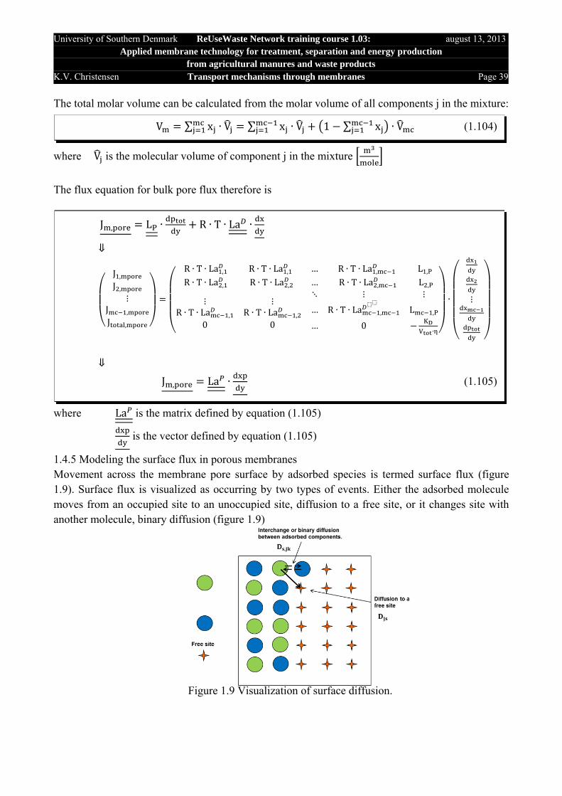
1.4.5 Modeling the surface flux in porous membranes Movement across the membrane pore surface by adsorbed species is termed surface flux (figure 1.9). Surface flux is visualized as occurring by two types of events. Either the adsorbed molecule moves from an occupied site to an unoccupied site, diffusion to a free site, or it changes site with another molecule, binary diffusion (figure 1.9)
Figure 1.9 Visualization of surface diffusion.
V ∑ x ∙ V ∑ x ∙ V 1 ∑ x ∙ V (1.104)
J , L ∙ R ∙ T ∙ La ∙
⇓
J ,J ,
⋮J ,
J ,
R ∙ T ∙ La , R ∙ T ∙ La ,
R ∙ T ∙ La , R ∙ T ∙ La ,
… R ∙ T ∙ La , L , … R ∙ T ∙ La , L ,
⋮ ⋮R ∙ T ∙ La , R ∙ T ∙ La ,
0 0
⋱ ⋮ ⋮
… R ∙ T ∙ La , L ,
… 0∙
∙ ⋮
⇓
J , La ∙ (1.105)

University of Southern Denmark ReUseWaste Network training course 1.03: august 13, 2013Applied membrane technology for treatment, separation and energy production
from agricultural manures and waste products K.V. Christensen Transport mechanisms through membranes Page 40
Krishna [5] has suggested modeling the surface flux on the line of the Stefan-Maxwell model for diffusion in gases. This leads to the following fundamental equation for the surface flux
where C , is the total number of moles of j that can be adsorbed per volume of membrane
D , is the binary surface diffusion coefficient between component j and k
D , is the surface diffusion coefficient between component j and an empty site
μ is the chemical potential for component j at the surface
θ is the fraction of surface sites covered by component j (see figure 1.10)
Figure 1.10 Visualization of surface coverage θ
Inorder to relate the chemical potential of component j adsorbed on the surface to the fluid bulk phase composition (liquid, vapor or gas) equilibrium between the fluid phase and the surface is assumed:
Where is the chemical potential of component j in the fluid mixture in the pore
Though thermodynamically stringent models for connecting the surface activity and spreading pressure with the chemical potential do exist they are at present of little practical value since methods for prediction of the surface activity and spreading pressure are not available yet. Instead a
∙∙ θ ∙ C , ∑
∙ , , ∙ , ,
,
, , (1.106)
(1.107)
University of Southern Denmark ReUseWaste Network training course 1.03: august 13, 2013Applied membrane technology for treatment, separation and energy production
from agricultural manures and waste products K.V. Christensen Transport mechanisms through membranes Page 41
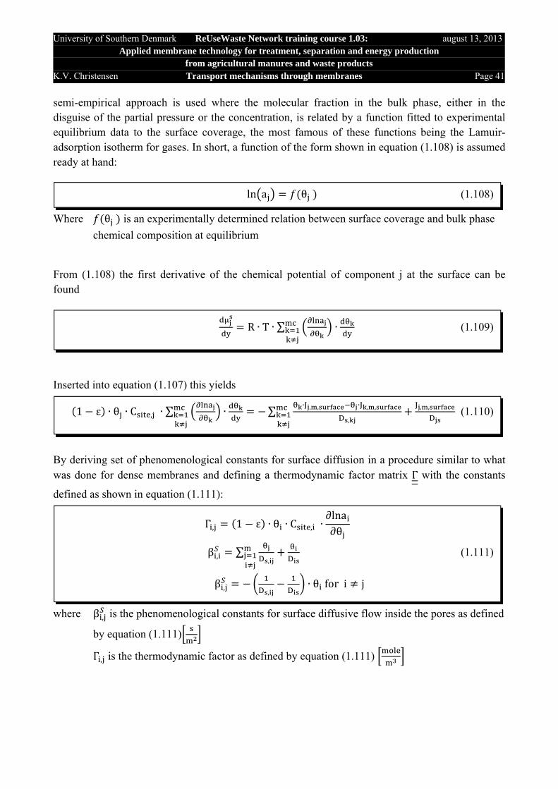
semi-empirical approach is used where the molecular fraction in the bulk phase, either in the disguise of the partial pressure or the concentration, is related by a function fitted to experimental equilibrium data to the surface coverage, the most famous of these functions being the Lamuir-adsorption isotherm for gases. In short, a function of the form shown in equation (1.108) is assumed ready at hand:
Where θ is an experimentally determined relation between surface coverage and bulk phase
chemical composition at equilibrium
From (1.108) the first derivative of the chemical potential of component j at the surface can be found
Inserted into equation (1.107) this yields
By deriving set of phenomenological constants for surface diffusion in a procedure similar to what was done for dense membranes and defining a thermodynamic factor matrix Γ with the constants
defined as shown in equation (1.111):
where β , is the phenomenological constants for surface diffusive flow inside the pores as defined
by equation (1.111)
Γ , is the thermodynamic factor as defined by equation (1.111)
ln a θ (1.108)
R ∙ T ∙ ∑ ∙ (1.109)
1 ε ∙ θ ∙ C , ∙ ∑ ∙ ∑∙ , , ∙ , ,
,
, , (1.110)
Γ , 1 ε ∙ θ ∙ C , ∙∂lna∂θ
β , ∑,
(1.111)
β ,,
∙ θ for i j
University of Southern Denmark ReUseWaste Network training course 1.03: august 13, 2013Applied membrane technology for treatment, separation and energy production
from agricultural manures and waste products K.V. Christensen Transport mechanisms through membranes Page 42
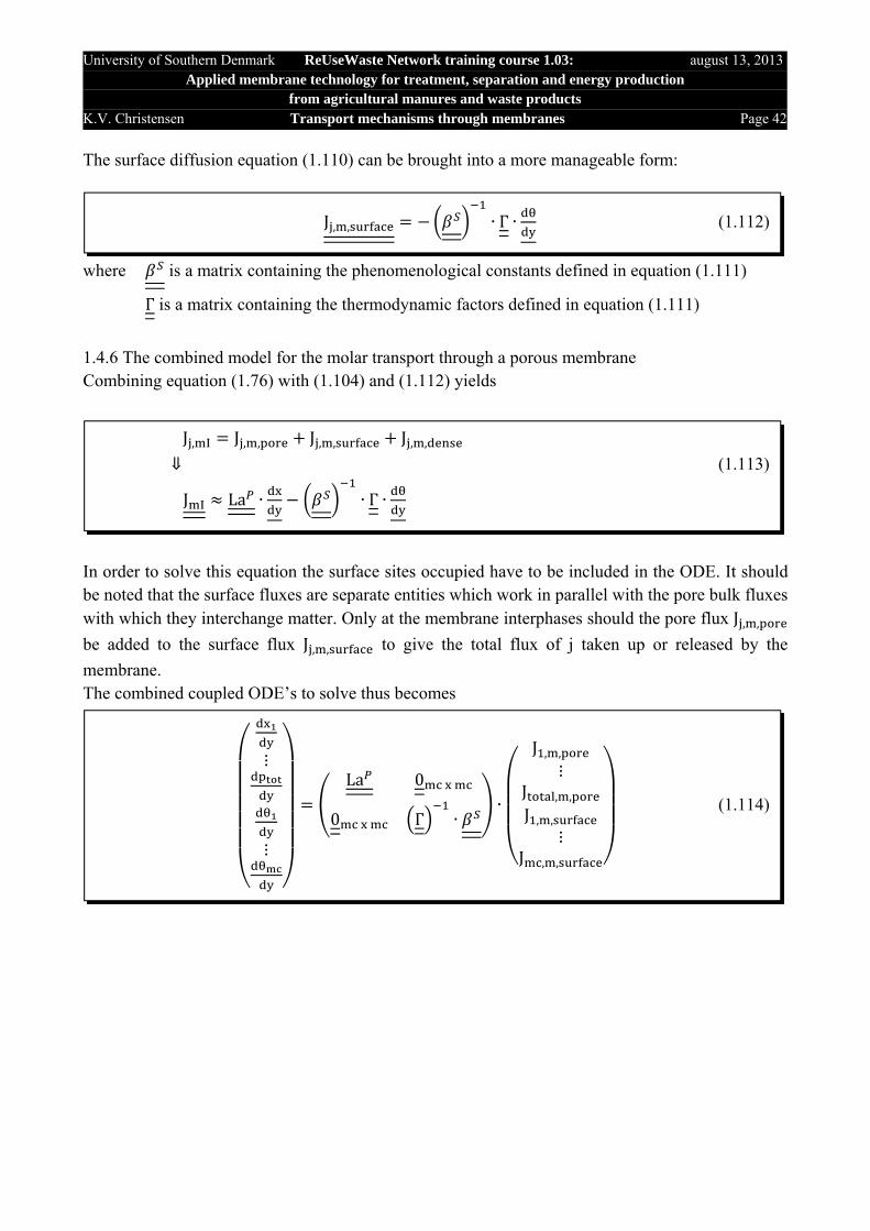
The surface diffusion equation (1.110) can be brought into a more manageable form:
where is a matrix containing the phenomenological constants defined in equation (1.111)
Γ is a matrix containing the thermodynamic factors defined in equation (1.111)
1.4.6 The combined model for the molar transport through a porous membrane Combining equation (1.76) with (1.104) and (1.112) yields
In order to solve this equation the surface sites occupied have to be included in the ODE. It should be noted that the surface fluxes are separate entities which work in parallel with the pore bulk fluxes with which they interchange matter. Only at the membrane interphases should the pore flux J , ,
be added to the surface flux J , , to give the total flux of j taken up or released by the
membrane. The combined coupled ODE’s to solve thus becomes
J , , ∙ Γ ∙ (1.112)
J , J , , J , , J , ,
⇓ (1.113)
J La ∙ ∙ Γ ∙
⋮
⋮
La 0
0 Γ ∙∙
J , ,
⋮J , ,
J , ,
⋮J , ,
(1.114)

University of Southern Denmark ReUseWaste Network training course 1.03: august 13, 2013Applied membrane technology for treatment, separation and energy production
from agricultural manures and waste products K.V. Christensen Transport mechanisms through membranes Page 43
The boundary conditions for equation (1.114) are
Equation (1.115) is quite intimidating and it is more often than not impossible to get all the data necessary for its use. Surface diffusion is still an area of intense research and diffusivity coefficients hard to come by or estimate. Fortunately for most practical applications, surface diffusion can be ignored and only the bulk transport equations are of interest. 1.4.7 Microfiltration Microfiltration membranes have distinctive if not well defined pores with mean pore diameters in the range between 0.1 and 10 μm depending on application. Microfiltration membranes are thus used primarily to remove minor particulate matter and microorganisms. In animal waste treatment they are typically used to remove microorganisms and smaller particulated matter not removed by screw press or centrifugation. As much phosphorous is bound to smaller particles in the liquid slurry fraction from manure or digestate, phosphorous will be partly concentrated in the retentate from the slurry. Potassium which is mostly dissolved in the liquid phase and nitrogen which is mostly bound as ammonium/ammonia, proteins and amino acids depending on the prehistory of the slurry will not be retained by the membrane. The flux through the pores will be totally dominated by the bulk flow and the surface diffusion term can safely be neglected. Further the convective flux will dominate the diffusive flux in the pores and as no appreciable concentration difference will normally occur for dissolved molecules, only convective flux need be considered. From a modeling point of view the individual fluxes thus can be calculated using D’Arcy’s law (equation 1.85):
From the pressure drop equation and the boundary conditions:
Boundarycondition:
x x , at y 0p p , at y 0
ln a , θ aty 0x x , aty ℓp p , at y 0
ln a , θ at y ℓ
(1.115)
J , C ∙ v C ∙ (1.85)
∙ (1.102)
Boundarycondition:p p , p , at y 0p p , p , at y ℓ

University of Southern Denmark ReUseWaste Network training course 1.03: august 13, 2013Applied membrane technology for treatment, separation and energy production
from agricultural manures and waste products K.V. Christensen Transport mechanisms through membranes Page 44
The velocity is found:
and the individual fluxes 1.116 with 1.85 becomes
As fouling and concentration polarization is a common problem in microfiltration the concentration of C , is often unknown and have to be accounted for before using equation (1.117).
1.4.8 Ultrafiltration Just as for microfiltration ultrafiltration membranes have distinctive if not well defined pores with mean pore diameters in the range between 2 and 100 nm depending on application. Ultrafiltration membranes are thus used primarily to remove minor particulate matter, microorganisms, vira, proteins and peptides. Often the feed to an ultrafiltration membrane might be prefiltered by microfiltration to avoid excessive particulate fouling of the membrane surface. The main purpose of ultrafiltration thus becomes to remove macromolecules. Therefore their pore size is often stated indirectly as the membranes Molecular Weight Cut Off (MWCO), the 90-% fractile molecular weight of the molecules that are allowed to parse the membrane. In animal waste treatment they are typically used to remove microorganisms, smaller particulate matter, vira and proteins not removed by screw press or centrifugation. Just as for microfiltration much phosphorous is bound to smaller particles in the liquid slurry fraction from manure or digestate, thus phosphorous will be partly concentrated in the retentate from the slurry. In digestate most proteins will have been degraded and nitrogen will pass the membrane as ammonia/ammonium and, if present, amino acids. For undigested slurry nitrogen in the form of proteins will be retained. Potassium which is mostly dissolved in the liquid phase will not be retained by the membrane.
∙
⇓
dp,
,
∙ dyℓ ∙ ∙ dy
ℓ
⇓ (1.116)
p , p ,∙ ∙ ℓ
⇓
v ∙ p , p ,
J , C , ∙ v C , ∙ ∙ p , p , (1.117)
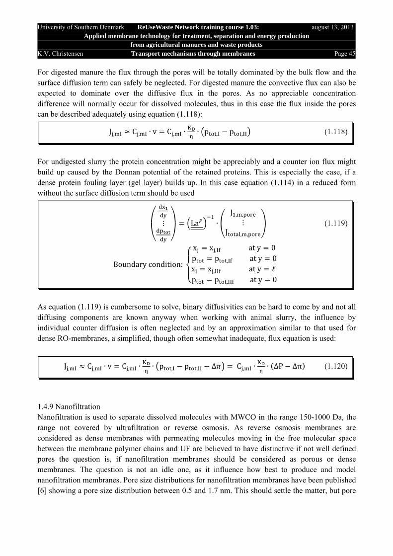
University of Southern Denmark ReUseWaste Network training course 1.03: august 13, 2013Applied membrane technology for treatment, separation and energy production
from agricultural manures and waste products K.V. Christensen Transport mechanisms through membranes Page 45
For digested manure the flux through the pores will be totally dominated by the bulk flow and the surface diffusion term can safely be neglected. For digested manure the convective flux can also be expected to dominate over the diffusive flux in the pores. As no appreciable concentration difference will normally occur for dissolved molecules, thus in this case the flux inside the pores can be described adequately using equation (1.118):
For undigested slurry the protein concentration might be appreciably and a counter ion flux might build up caused by the Donnan potential of the retained proteins. This is especially the case, if a dense protein fouling layer (gel layer) builds up. In this case equation (1.114) in a reduced form without the surface diffusion term should be used
As equation (1.119) is cumbersome to solve, binary diffusivities can be hard to come by and not all diffusing components are known anyway when working with animal slurry, the influence by individual counter diffusion is often neglected and by an approximation similar to that used for dense RO-membranes, a simplified, though often somewhat inadequate, flux equation is used:
1.4.9 Nanofiltration Nanofiltration is used to separate dissolved molecules with MWCO in the range 150-1000 Da, the range not covered by ultrafiltration or reverse osmosis. As reverse osmosis membranes are considered as dense membranes with permeating molecules moving in the free molecular space between the membrane polymer chains and UF are believed to have distinctive if not well defined pores the question is, if nanofiltration membranes should be considered as porous or dense membranes. The question is not an idle one, as it influence how best to produce and model nanofiltration membranes. Pore size distributions for nanofiltration membranes have been published [6] showing a pore size distribution between 0.5 and 1.7 nm. This should settle the matter, but pore
J , C , ∙ v C , ∙ ∙ p , p , (1.118)
Boundarycondition:
x x , aty 0p p , aty 0x x , at y ℓp p , at y 0
⋮ La ∙J , ,
⋮J , ,
(1.119)
J , C , ∙ v C , ∙ ∙ p , p , ∆ C , ∙ ∙ ∆P ∆π (1.120)
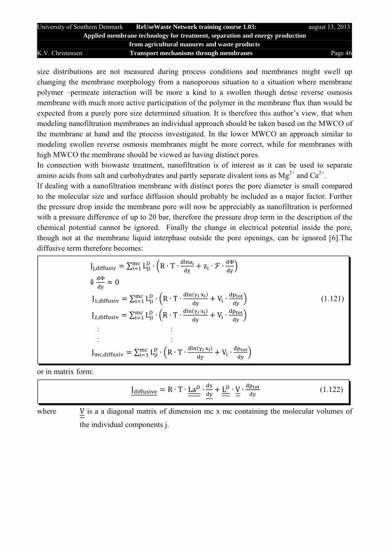
University of Southern Denmark ReUseWaste Network training course 1.03: august 13, 2013Applied membrane technology for treatment, separation and energy production
from agricultural manures and waste products K.V. Christensen Transport mechanisms through membranes Page 46
size distributions are not measured during process conditions and membranes might swell up changing the membrane morphology from a nanoporous situation to a situation where membrane polymer –permeate interaction will be more a kind to a swollen though dense reverse osmosis membrane with much more active participation of the polymer in the membrane flux than would be expected from a purely pore size determined situation. It is therefore this author’s view, that when modeling nanofiltration membranes an individual approach should be taken based on the MWCO of the membrane at hand and the process investigated. In the lower MWCO an approach similar to modeling swollen reverse osmosis membranes might be more correct, while for membranes with high MWCO the membrane should be viewed as having distinct pores. In connection with biowaste treatment, nanofiltration is of interest as it can be used to separate amino acids from salt and carbohydrates and partly separate divalent ions as Mg2+ and Ca2+. If dealing with a nanofiltration membrane with distinct pores the pore diameter is small compared to the molecular size and surface diffusion should probably be included as a major factor. Further the pressure drop inside the membrane pore will now be appreciably as nanofiltration is performed with a pressure difference of up to 20 bar, therefore the pressure drop term in the description of the chemical potential cannot be ignored. Finally the change in electrical potential inside the pore, though not at the membrane liquid interphase outside the pore openings, can be ignored [6].The diffusive term therefore becomes:
or in matrix form:
where V is a a diagonal matrix of dimension mc x mc containing the molecular volumes of
the individual components j.
J , ∑ L ∙ R ∙ T ∙ z ∙ ∙
⇓ 0
J , ∑ L ∙ R ∙ T ∙ ∙ V ∙ (1.121)
J , ∑ L ∙ R ∙ T ∙ ∙ V ∙
: : : :
J , ∑ L ∙ R ∙ T ∙ ∙ V ∙
J R ∙ T ∙ La ∙ L ∙ V ∙ (1.122)
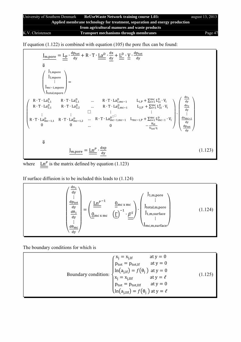
University of Southern Denmark ReUseWaste Network training course 1.03: august 13, 2013Applied membrane technology for treatment, separation and energy production
from agricultural manures and waste products K.V. Christensen Transport mechanisms through membranes Page 47
If equation (1.122) is combined with equation (105) the pore flux can be found:
where Ln is the matrix defined by equation (1.123)
If surface diffusion is to be included this leads to (1.124)
The boundary conditions for which is
J , L ∙ R ∙ T ∙ La ∙ L ∙ V ∙
⇓
J ,J ,
⋮J ,
J ,
R ∙ T ∙ La , R ∙ T ∙ La ,
R ∙ T ∙ La , R ∙ T ∙ La ,
… R ∙ T ∙ La , L , ∑ L ∙ V … R ∙ T ∙ La , L , ∑ L ∙ V
⋮ ⋮R ∙ T ∙ La , R ∙ T ∙ La ,
0 0
⋮ ⋮
… R ∙ T ∙ La , L , ∑ L ∙ V
… 0∙
∙ ⋮
⇓
J , Ln ∙ (1.123)
⋮
⋮
Ln 0
0 Γ ∙∙
J , ,
⋮J , ,
J , ,
⋮J , ,
(1.124)
Boundarycondition:
x x , at y 0p p , at y 0
ln a , θ aty 0x x , aty ℓp p , at y 0
ln a , θ at y ℓ
(1.125)
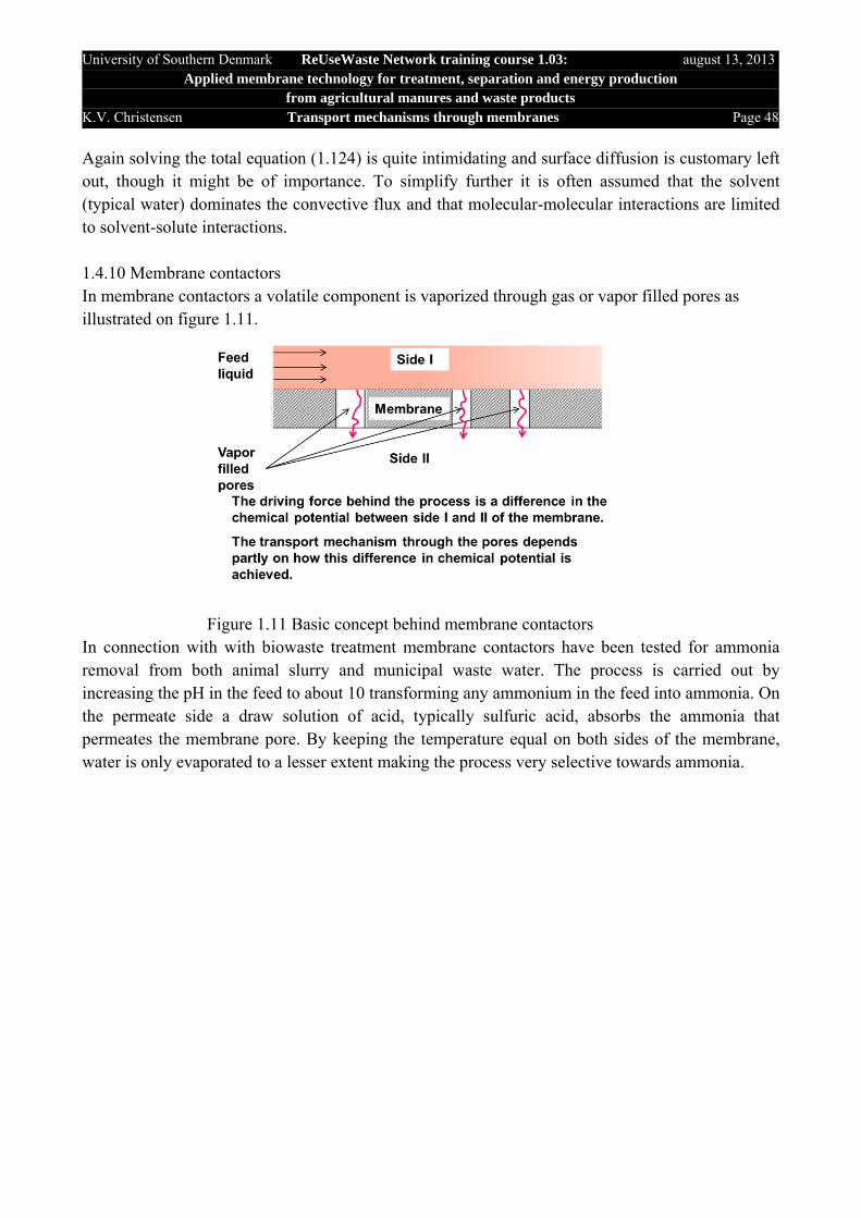
University of Southern Denmark ReUseWaste Network training course 1.03: august 13, 2013Applied membrane technology for treatment, separation and energy production
from agricultural manures and waste products K.V. Christensen Transport mechanisms through membranes Page 48
Again solving the total equation (1.124) is quite intimidating and surface diffusion is customary left out, though it might be of importance. To simplify further it is often assumed that the solvent (typical water) dominates the convective flux and that molecular-molecular interactions are limited to solvent-solute interactions. 1.4.10 Membrane contactors In membrane contactors a volatile component is vaporized through gas or vapor filled pores as illustrated on figure 1.11.
Figure 1.11 Basic concept behind membrane contactors
In connection with with biowaste treatment membrane contactors have been tested for ammonia removal from both animal slurry and municipal waste water. The process is carried out by increasing the pH in the feed to about 10 transforming any ammonium in the feed into ammonia. On the permeate side a draw solution of acid, typically sulfuric acid, absorbs the ammonia that permeates the membrane pore. By keeping the temperature equal on both sides of the membrane, water is only evaporated to a lesser extent making the process very selective towards ammonia.
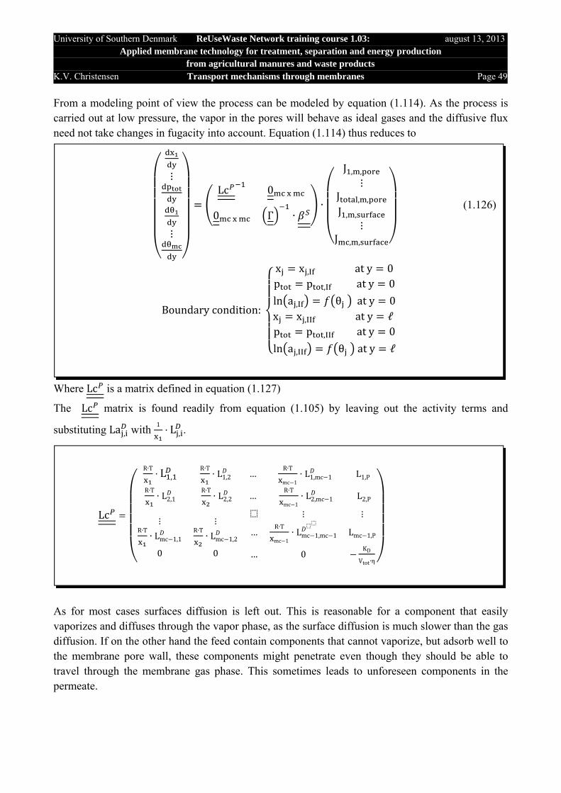
University of Southern Denmark ReUseWaste Network training course 1.03: august 13, 2013Applied membrane technology for treatment, separation and energy production
from agricultural manures and waste products K.V. Christensen Transport mechanisms through membranes Page 49
From a modeling point of view the process can be modeled by equation (1.114). As the process is carried out at low pressure, the vapor in the pores will behave as ideal gases and the diffusive flux need not take changes in fugacity into account. Equation (1.114) thus reduces to
Where Lc is a matrix defined in equation (1.127)
The Lc matrix is found readily from equation (1.105) by leaving out the activity terms and
substituting La , with 1∙ L , .
As for most cases surfaces diffusion is left out. This is reasonable for a component that easily vaporizes and diffuses through the vapor phase, as the surface diffusion is much slower than the gas diffusion. If on the other hand the feed contain components that cannot vaporize, but adsorb well to the membrane pore wall, these components might penetrate even though they should be able to travel through the membrane gas phase. This sometimes leads to unforeseen components in the permeate.
Boundarycondition:
x x , aty 0p p , aty 0
ln a , θ aty 0x x , aty ℓp p , aty 0
ln a , θ at y ℓ
⋮
⋮
Lc 0
0 Γ ∙∙
J , ,
⋮J , ,
J , ,
⋮J , ,
(1.126)
Lc
R∙T∙ L ,
R∙T∙ L1,2
R∙T∙ L2,1
R∙T∙ L2,2
…R∙T
mc 1∙ L1,mc 1 L1,P
…R∙T
mc 1∙ L2,mc 1 L2,P
⋮ ⋮R∙T
∙ Lmc 1,1R∙T
∙ Lmc 1,2
0 0
⋮ ⋮
…R∙T
mc 1∙ Lmc 1,mc 1 Lmc 1,P
… 0KD
Vtot∙η
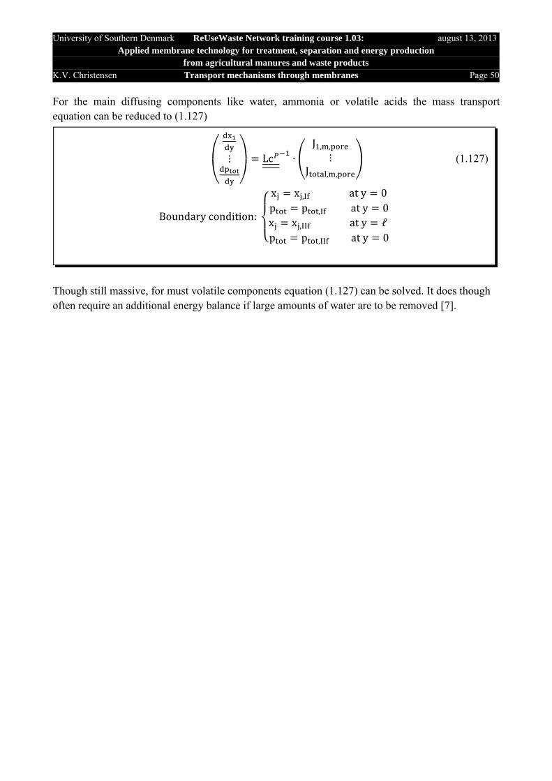
University of Southern Denmark ReUseWaste Network training course 1.03: august 13, 2013Applied membrane technology for treatment, separation and energy production
from agricultural manures and waste products K.V. Christensen Transport mechanisms through membranes Page 50
For the main diffusing components like water, ammonia or volatile acids the mass transport equation can be reduced to (1.127)
Though still massive, for must volatile components equation (1.127) can be solved. It does though often require an additional energy balance if large amounts of water are to be removed [7].
Boundarycondition:
x x , aty 0p p , aty 0x x , aty ℓp p , at y 0
⋮ Lc ∙J , ,
⋮J , ,
(1.127)
University of Southern Denmark ReUseWaste Network training course 1.03: august 13, 2013Applied membrane technology for treatment, separation and energy production
from agricultural manures and waste products K.V. Christensen Transport mechanisms through membranes Page 51
List of Symbols
A is the film surface area at side I of the membrane m A is the film surface area at side II of the membrane m
A is the solvent permeability constant defined by equation (1.58)
∙ ∙
A is the membrane surface area at side I of the membrane m A is the scaling/fouling layer surface area at side I of the membrane m A is the scaling/fouling layer surface area at side II of the membrane m a is the activity of component j in the mixture
a , is the activity of component j in the mixture outside the membrane at interface II
a , is the activity of component j in the membrane at interface II
B is the solute permeability constant defined by equation (1.60)
C is the molar concentration of j
C , is the concentration of j outside membrane at position y = 0 (fig. 1.4)
C , is the concentration of j outside membrane at position y = ℓ (fig. 1.4)
C , is the concentration of j inside membrane at position y = 0 (fig. 1.4)
C , is the concentration of j inside membrane at position y = ℓ (fig. 1.4)
C , is the total number of moles of j that can be adsorbed per volume of membrane
C is the total molar concentration of j
C , is the total concentration in the membrane
D is the binary diffusion coefficient for component i and j
D , is the surface diffusion coefficient between component j and an empty site
D , is the Knudsen diffusion coefficient
D , is the diffusion coefficient for j relative to the membrane
D , is the binary diffusion coefficient for component i and j inside the membrane
D , is the binary surface diffusion coefficient between component j and k
D , is the thermal diffusivity ∙
dp is the diameter of the original sinter pellets from which the membrane was made [m]
is a a vector of dimension m containing the individual derivatives of lnai as defined by equation
(1.33)

University of Southern Denmark ReUseWaste Network training course 1.03: august 13, 2013Applied membrane technology for treatment, separation and energy production
from agricultural manures and waste products K.V. Christensen Transport mechanisms through membranes Page 52
is a a vector of dimension m containing the individual derivatives of xi
is the vector defined by equation (1.105)
dp is the diameter of the original sinter pellets [m] E is a diagonal unit matrix
is Faradays constant 9.64853 ∙ 10 C
mole
f is the fugacity of pure j Pa
f is the fugacity of j in the mixture Pa
f is the fugacity of j in its standard state Pa
f , is the fugacity of component j in the mixture outside the membrane at interface II [Pa]
f , is the fugacity of component j in the gas phase at conditions outside the membrane at interface
II [Pa]
f , ℓ is the fugacity of component j in the liquid phase at conditions outside the membrane at
interface II [Pa]
f , is the fugacity of component j in the mixture in the membrane at interface II [Pa]
G is the molar Gibbs free energy of the fluid mixture
J , is the convective molar flux of component j through the porous part of the
membrane
∙
J , is the diffusive molar flux of component j through the poros part of the
membrane
∙
J , is the molar flux of component j through the film layer at side I
∙
J , is the molar flux of component j through the film layer at side II
∙
J , , is the overall molar flux of component j through the membrane
∙
J , , is the molar flux of component j through the dense part of the pore based on the area of
side I
∙
J , , is the molar flux of component j through the membrane pore based on the area of side
∙
J , , is the molar flux of component j on the membrane pore surface based on the area of side
I
∙
J , is the molar flux of component j through the membrane based on the area of side I
∙
J , , is the molar flux of component j through the membrane based on the area of side I
caused by convection
∙

University of Southern Denmark ReUseWaste Network training course 1.03: august 13, 2013Applied membrane technology for treatment, separation and energy production
from agricultural manures and waste products K.V. Christensen Transport mechanisms through membranes Page 53
J , , is the flux of j through the membrane at equilibrium
∙
J , is the molar flux of component j through the scaling/fouling layer at side I
∙
J , is the molar flux of component j through the scaling/fouling layer at side II
∙
J , is the thermal molar flux of component j through the poros part of the
membrane
∙
J , , is the molar flux of component j on the membrane pore surface based on the area of side
I
∙
J is a vector of the dimension m containing the individual flux values
K is a shape constant based on the sinter particles KD is the D’Arcy constants [m2] K , is distribution coefficient of concentration of j at position y = 0
K , is distribution coefficient of concentration of j at position y = ℓ
L is an m x m matrix containing the individual proportionality constants as defined by equation
(1.34) L is an m x m matrix containing the individual diffusive proportionality constants as defined by
equation (1.93) L is the proportionality constant for the molar flux of component j relative to the driving force k
L is a diagonal matrix containing the pressure proportionality constants as defined in equation
(1.100) L is a diagonal matrix containing the temperature proportionality constants as defined in equation
(1.101) La is an mc x mc matrix containing the individual proportionality constants as defined by equation
(1.47) La is an mc x mc matrix containing the individual proportionality constants as defined by equation
(1.97) La is the matrix defined by equation (1.105)
Lc is a matrix defined in equation (1.127)
ℓ is the thickness of the membrane m
M , is the molecular weight of component j
m is the total number of components present including the membrane mc is the total number of components present inside the membrane excluding the membrane mf is the number of driving forces n is the total number of moles mole n is the of moles of component j moleofj

University of Southern Denmark ReUseWaste Network training course 1.03: august 13, 2013Applied membrane technology for treatment, separation and energy production
from agricultural manures and waste products K.V. Christensen Transport mechanisms through membranes Page 54
P is the permeability coefficient of j
p , is the partial pressure of j in the mixture outside the membrane at interface I [Pa]
p , is the partial pressure of j in the mixture outside the membrane at interface II [Pa]
p is vapor pressure of pure j at the process temperature [Pa]
p is the total pressure Pa p , is the pressure in chamber I [Pa]
p , , is the pressure in chamber I at equilibrium [Pa]
p , is the pressure in chamber II [Pa]
p , , is the pressure in chamber II at equilibrium [Pa]
p , is the pressure in the mixture outside the membrane at interface II [Pa]
p , is the pressure in the membrane at interface II [Pa]
P is the permeability coefficient of j
R is the universal gas constant, 8.314∙
r is the pore mean radius [m]
S is the of molar volume entropy of the mixture
s is the internal surface area of the pore [m2] sf is the sphericity of the original sinter pellet from which the membrane was made T is the temperature K V is a a diagonal matrix of dimension mc x mc containing the molecular volumes of the individual
components j.
V is a vector containing the molecular volume of all components j in the mixture
V is the molecular volume of pure j
V is the molecular volume of component j in the mixture
V is the of molar volume of the mixture
v is the velocity of the fluid
X is the driving force k x is a diagonal matrix holding the molecular fractions xi in its diagonal
x is the molecular fraction of j in the mixture
y the distance travelled through the membrane perpendicular to the membrane surface [m] Z is a diagonal m x m matrix containing the individual molecular charges as seen in equation (1.35)
z is the electric charge of ion i β is a phenomenological constant which for purely molecular diffusivity is defined by equation
(1.40)
University of Southern Denmark ReUseWaste Network training course 1.03: august 13, 2013Applied membrane technology for treatment, separation and energy production
from agricultural manures and waste products K.V. Christensen Transport mechanisms through membranes Page 55
β , is the phenomenological constants for diffusive bulk flow inside the pores as defined by
equation (1.92)
β , is the phenomenological constants for surface diffusive flow inside the pores as defined by
equation (1.111)
∆P is the pressure difference between chamber I and II [Pa] ∆ is the osmotic pressure difference between camber I and II [Pa]
Γ , is the thermodynamic factor as defined by equation (1.111)
γ is the activity coefficient j in the mixture
γ , is the activity coefficient of j in the mixture outside the membrane at interface II
γ , ℓ is the activity coefficient of component j in the liquid phase at conditions outside the
membrane at interface I γ , is the activity coefficient of j in the mixture outside the membrane at interface II
γ , is the activity coefficient of j in the membrane at interface I
γ , is the activity coefficient of j in the membrane at interface II
η is the viscosity of the fluid Pa ∙ s Φ is the electrical potential V Φ is the electrical potential in the mixture outside the membrane at interface II V Φ is the electrical potential in the mixture in the membrane at interface II V
φ is fugacity coefficient of pure j at the process temperature and pressure
φ , is the fugacity coefficient of j in the mixture outside the membrane at interface I
φ , is the fugacity coefficient of component j in the gas phase at conditions outside the membrane
at interface I φ , ℓ is the fugacity coefficient of component j in the liquid phase at conditions outside the
membrane at interface I φ , is the fugacity coefficient of j in the mixture outside the membrane at interface II
is electrochemical potential of component j in the mixture
is the standard chemical potential of component j
, is the chemical potential of component j in the mixture outside the membrane at interface II
, is the chemical potential of component j in the membrane at interface II
is the chemical potential of component j in the fluid mixture in the pore
μ is the chemical potential for component j at the surface
τ is the tortuosity θ is the fraction of surface sites covered by component j (see figure 1.10)
University of Southern Denmark ReUseWaste Network training course 1.03: august 13, 2013Applied membrane technology for treatment, separation and energy production
from agricultural manures and waste products K.V. Christensen Transport mechanisms through membranes Page 56
Literature
1. J.M. Smith, H.C. van Ness, M.M. Abbott: Introduction to chemical engineering thermodynamics, 7th Ed., McGraw-Hill, Singapore, 2005
2. D.R. Poul: The Solution Diffusion Model for Swollen Membranes, Separation and Purification, vol. 5, 33-50, 1976.
3. J.M. Coulson, J.F. Richardson, J.R. Backhurst, J.H. Harker: Richardson & Coulson’s Chemical Engineering Vol. 1, 6th Ed., Butterworth-Heinemann, 1999, Oxford
4. K.K.Y. Kuo: Principles of combustion, John Wiley and Sons, New York 1968.
5. R. Krishna: Multicomponent surface Diffusion of adsorbed species: A description based on the generalized Mawell-Stefan equations, Chemical Engineering Science, vol. 45, 1779-1791, 1990.
6. A. I. Schäfer, A.G.Fane, T.D. Waite Nanofiltration – Principles and Applications, Elsevier, Oxford UK, 2005
7. M.B. Jensen, K.V. Christensen, R. Andresen, L.F. Søtoft, B. Norddahl A model of direct contact membrane distillation for black currant juice, Journal of Food Engineering, vol. 107, 405-414.