Transport: Non-diffusive, flux conservative initial value problems and

Chapter 5

Transport: Non-diffusive, fluxconservative initial valueproblems and how to solve them

Selected Reading

Numerical Recipes, 2nd edition: Chapter 19

A. Staniforth and J. Cote. Semi-Lagrangian integration schemes for atmosphericmodels - a review, Monthly Weather Review 119, 2206–2223, Sep 1991.

5.1 Introduction

This chapter will consider the physics and solution of the simplest partial differen-tial equations for flux conservative transport such as the continuity equation

∂ρ

∂t+ ∇· ρV = 0 (5.1.1)

We will begin by demonstrating the physical implications ofthese sorts of equa-tions, show that they imply non-diffusive transport and discuss the meaning ofthe material derivative. We will then demonstrate the relationship between thesePDE’s and the ODE’s of the previous sections and demonstrateparticle methodsof solution. We’ll discuss the pros and cons of particle methods and then showhow to solve these equations using simple finite difference methods. We will alsoshow that these equations are perhaps the most difficult to solve accurately on afixed grid. By the time we are done, I hope you will instinctively think transportwhenever you see an equation or terms of this form.

53

54

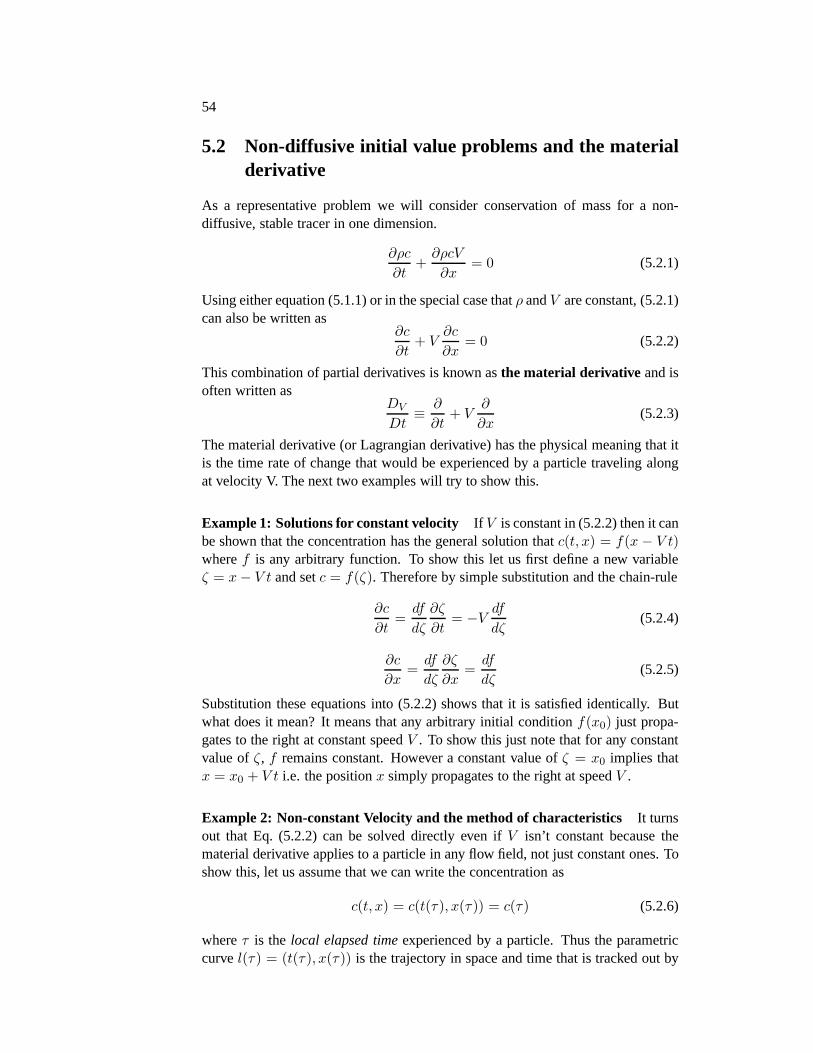
5.2 Non-diffusive initial value problems and the materialderivative

As a representative problem we will consider conservation of mass for a non-diffusive, stable tracer in one dimension.

∂ρc

∂t+

∂ρcV

∂x= 0 (5.2.1)

Using either equation (5.1.1) or in the special case thatρ andV are constant, (5.2.1)can also be written as

∂c

∂t+ V

∂c

∂x= 0 (5.2.2)

This combination of partial derivatives is known asthe material derivative and isoften written as

DV

Dt≡

∂

∂t+ V

∂

∂x(5.2.3)

The material derivative (or Lagrangian derivative) has thephysical meaning that itis the time rate of change that would be experienced by a particle traveling alongat velocity V. The next two examples will try to show this.

Example 1: Solutions for constant velocity If V is constant in (5.2.2) then it canbe shown that the concentration has the general solution that c(t, x) = f(x − V t)wheref is any arbitrary function. To show this let us first define a newvariableζ = x − V t and setc = f(ζ). Therefore by simple substitution and the chain-rule

∂c

∂t=

df

dζ

∂ζ

∂t= −V

df

dζ(5.2.4)

∂c

∂x=

df

dζ

∂ζ

∂x=

df

dζ(5.2.5)

Substitution these equations into (5.2.2) shows that it is satisfied identically. Butwhat does it mean? It means that any arbitrary initial condition f(x0) just propa-gates to the right at constant speedV . To show this just note that for any constantvalue ofζ, f remains constant. However a constant value ofζ = x0 implies thatx = x0 + V t i.e. the positionx simply propagates to the right at speedV .

Example 2: Non-constant Velocity and the method of characteristics It turnsout that Eq. (5.2.2) can be solved directly even ifV isn’t constant because thematerial derivative applies to a particle in any flow field, not just constant ones. Toshow this, let us assume that we can write the concentration as

c(t, x) = c(t(τ), x(τ)) = c(τ) (5.2.6)

whereτ is the local elapsed timeexperienced by a particle. Thus the parametriccurvel(τ) = (t(τ), x(τ)) is the trajectory in space and time that is tracked out by

Transport equations 55

the particle. If we now ask, what is the change in concentration with τ along thepath we get

dc

dτ=

∂c

∂t

dt

dτ+

∂c

∂x

dx

dτ(5.2.7)

Comparison of (5.2.7) to (5.2.2) shows that (5.2.2) can actually be written as acoupled set of ODE’s.

dc

dτ= 0 (5.2.8)

dt

dτ= 1 (5.2.9)

dx

dτ= V (5.2.10)

Which state that the concentration of the particle remains constant along the path,the local time and the global time are equivalent and the change in position of theparticle with time is given by the Velocity. The important point is that if V (x, t)is known, Eqs. (5.2.8)–(5.2.10) can be solved with all the sophisticated techniquesfor solving ODE’s. Many times they can be solved analytically. This method iscalled the method of characteristicswhere the characteristics are the trajectoriestraced out in time and space.

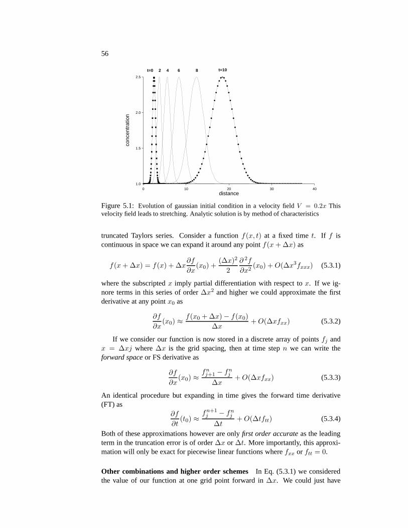
Particle based methods The previous sections suggest that one manner of solv-ing non-diffusive transport problems is to simply approximate your initial condi-tion as a set of discrete particles and track the position of the particles through time.As long as the interaction between particles does not dependon spatial gradients(e.g. diffusion) this technique is actually very powerful.Figure 5.1 shows the ana-lytic solution forc given a gaussian initial condition andV = 0.2x. This method isquite general, can be used for non-linear equations (shock waves) and for problemswith source and sink terms such as radioactive decay (as longas the source termis independent of other characteristics). If you just want to track things accuratelythrough a flow field it may actually be the preferred method of solution. However,if there are lots of particles or you have several species whointeract with eachother, then you will need to interpolate between particles and the method becomesvery messy. For these problems you may want to try aEuleriangrid-based method.These methods, of course, have their own problems. When we’re done discussingall the pitfalls of grid-based advection schemes we will come back and discuss apotentially very powerful hybrid method calledsemi-lagrangian schemeswhichcombine the physics of particle based schemes with the convenience of uniformgrids.

5.3 Grid based methods and simple finite differences

The basic idea behind Finite-difference, grid-based methods is to slap a static gridover the solution space and to approximate the partial differentials at each pointin the grid. The standard approach for approximating the differentials comes from

56

0 10 20 30 40distance

1.0

1.5

2.0

2.5

conc

entr

atio

n

t=0 2 4 6 8 t=10

Figure 5.1: Evolution of gaussian initial condition in a velocity fieldV = 0.2x Thisvelocity field leads to stretching. Analytic solution is by method of characteristics

truncated Taylors series. Consider a functionf(x, t) at a fixed timet. If f iscontinuous in space we can expand it around any pointf(x + ∆x) as

f(x + ∆x) = f(x) + ∆x∂f

∂x(x0) +

(∆x)2

2

∂ 2f

∂x2(x0) + O(∆x3fxxx) (5.3.1)

where the subscriptedx imply partial differentiation with respect tox. If we ig-nore terms in this series of order∆x2 and higher we could approximate the firstderivative at any pointx0 as

∂f

∂x(x0) ≈

f(x0 + ∆x) − f(x0)

∆x+ O(∆xfxx) (5.3.2)

If we consider our function is now stored in a discrete array of points fj andx = ∆xj where∆x is the grid spacing, then at time stepn we can write theforward spaceor FS derivative as

∂f

∂x(x0) ≈

fnj+1 − fn

j

∆x+ O(∆xfxx) (5.3.3)

An identical procedure but expanding in time gives the forward time derivative(FT) as

∂f

∂t(t0) ≈

fn+1j − fn

j

∆t+ O(∆tftt) (5.3.4)

Both of these approximations however are onlyfirst order accurateas the leadingterm in the truncation error is of order∆x or ∆t. More importantly, this approxi-mation will only be exact for piecewise linear functions where fxx or ftt = 0.

Other combinations and higher order schemes In Eq. (5.3.1) we consideredthe value of our function at one grid point forward in∆x. We could just have


easily taken a step backwards to get

f(x − ∆x) = f(x) − ∆x∂f

∂x(x0) +

(∆x)2

2

∂ 2f

∂x2(x0) − O(∆x3fxxx) (5.3.5)

If we truncate at order∆x2 and above we still get a first order approximation fortheBackward space step(BS)

∂f

∂x(x0) ≈

fnj − fn

j−1

∆x− O(∆xfxx) (5.3.6)

which isn’t really any better than the forward step as it has the same order error (butof opposite sign). We can do a fair bit better however if we combine Eqs. (5.3.1)and (5.3.5) to remove the equal but opposite 2nd order terms.If we subtract (5.3.5)from (5.3.1) and rearrange, we can get thecentered space(CS) approximation

∂f

∂x(x0) ≈

fnj+1 − fn

j−1

2∆x− O(∆x2fxxx) (5.3.7)

Note we have still only used two grid points to approximate the derivative but havegained an order in the truncation error. By including more and more neighboringpoints, even higher order schemes can be dreamt up (much likethe 4th order RungeKutta ODE scheme), however, the problem of dealing with large patches of pointscan become bothersome, particularly at boundaries. By the way, we don’t have tostop at the first derivative but we can also come up with approximations for thesecond derivative (which we will need shortly). This time, by adding (5.3.1) and(5.3.5) and rearranging we get

∂ 2f

∂x2(x0) ≈

fnj+1 − 2fn

j + fnj−1

(∆x)2+ O(∆x2fxxxx) (5.3.8)

This form only needs a point and its two nearest neighbours. Note that while thetruncation error is of order∆x2 it is actually a 3rd order scheme because a cubicpolynomial would satisfy it exactly (i.e.fxxxx = 0). B.P. Leonard [1] has a fieldday with this one.

5.3.1 Another approach to differencing: polynomial interpolation

In the previous discussion we derived several difference schemes by combiningvarious truncated Taylor series to form an approximation todifferentials of differ-ent orders. The trick is to combine things in just the right way to knock out variouserror terms. Unfortunately, this approach is not particularly intuitive and can behard to sort out for more arbitrary grid schemes or higher order methods. Nev-ertheless, the end product is simply a weighted combinationof the values of ourfunction at neighbouring points. This section will developa related technique thatis essentially identical but it is general and easy to modify.

The important point of these discretizations is that they are all effectively as-suming that the our function can be described by a truncated Taylor’s series. How-ever, we also know that polynomials of fixed order can also be described exactly

58

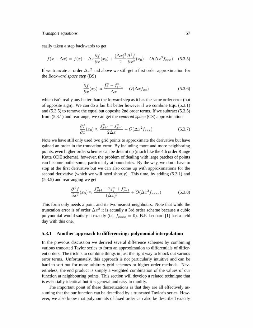
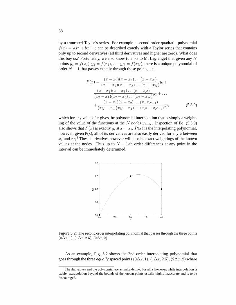
by a truncated Taylor’s series. For example a second order quadratic polynomialf(x) = ax2 + bx + c can be described exactly with a Taylor series that containsonly up to second derivatives (all third derivatives and higher are zero). What doesthis buy us? Fortunately, we also know (thanks to M. Lagrange) that given anyNpointsy1 = f(x1), y2 = f(x2), . . . , yN = f(xN ), there is a unique polynomial oforderN − 1 that passes exactly through those points, i.e.

P (x) =(x − x2)(x − x3) . . . (x − xN )

(x1 − x2)(x1 − x3) . . . (x1 − xN )y1+

(x − x1)(x − x3) . . . (x − xN )

(x2 − x1)(x2 − x3) . . . (x2 − xN )y2 + . . .

+(x − x1)(x − x2) . . . (x−xN−1)

(xN − x1)(xN − x2) . . . (xN − xN−1)yN (5.3.9)

which for any value ofx gives the polynomial interpolation that is simply a weight-ing of the value of the functions at theN nodesy1...N . Inspection of Eq. (5.3.9)also shows thatP (x) is exactlyyi atx = xi. P (x) is the interpolating polynomial,however, given P(x), all of its derivatives are also easily derived for anyx betweenx1 andxN

1 These derivatives however will also be exact weightings of the knownvalues at the nodes. Thus up toN − 1-th order differences at any point in theinterval can be immediately determined.

0.0 0.5 1.0 1.5 2.0

x

1.0

1.5

2.0

2.5

3.0

f(x)

Figure 5.2:The second order interpolating polynomial that passes through the three points(0∆x, 1), (1∆x, 2.5), (2∆x, 2)

As an example, Fig. 5.2 shows the 2nd order interpolating polynomial thatgoes through the threeequallyspaced points(0∆x, 1), (1∆x, 2.5), (2∆x, 2) where

1The derivatives and the polynomial are actually defined for all x however, while interpolation isstable, extrapolation beyond the bounds of the known pointsusually highly inaccurate and is to bediscouraged.


x = i∆x (note:i need not be an integer). Using Eq. 5.3.9) then yields

P (x) =(i − 1)(i − 2)

2f0 +

(i − 0)(i − 2)

−1f1 +

(i − 0)(i − 1)

2f2(5.3.10)

P ′(x) =1

∆x

[

(i − 1) + (i − 2)

2f0 +

i + (i − 2)

−1f1 +

i + (i − 1)

2f2

]

(5.3.11)

P ′′(x) =1

∆x2[f0 − 2f1 + f2] (5.3.12)

whereP ′ andP ′′ are the first and second derivatives. Thus using Eq. (5.3.11),thefirst derivative of the polynomial at the center point is

P ′(x = ∆x) =1

∆x

[

−1

2f0 +

1

2f2

]

(5.3.13)

which is identical to the centered difference given by Eq. (5.3.7). As a shorthandwe will often write this sort of weighting scheme as astencillike

∂f

∂x≈

1

∆x

[

−1/2 0 1/2]

f (5.3.14)

where a stencil is an operation at a point that involves some number of nearestneighbors. Just for completeness, here are the 2nd order stencils for the first deriva-tive at several points

fx =1

∆x

[

−3/2 2 −1/2]

atx = 0 (5.3.15)

fx =1

∆x

[

−1 1 0]

atx = 1/2∆x (5.3.16)

fx =1

∆x

[

0 −1 1]

atx = 3/2∆x (5.3.17)

fx =1

∆x

[

1/2 −2 3/2]

atx = 2∆x (5.3.18)

Note as a check, the weightings of the stencil for any derivative should sum tozero because the derivatives of a constant are zero. The second derivative stencil isalways

fxx =1

∆x2

[

1 −2 1]

(5.3.19)

for all points in the interval because the 2nd derivative of aparabola is constant.Generalizing to higher order schemes just requires using more points to define thestencil. Likewise it is straightforward to work out weighting schemes for unevenlyspaced grid points.

5.3.2 Putting it all together

Given all the different approximations for the derivatives, the art of finite-differencingis putting them together in stable and accurate combinations. Actually it’s not re-ally an art but common sense given a good idea of what the actual truncation error

60

is going to do to you. As an example, I will show you a simple, easily coded and to-tally unstable technique known asforward-time centered spaceor simply the FTCSmethod. If we consider the canonical 1-D transport equationwith constant veloci-ties (5.2.2) and replace the time derivative with a FT approximation and the spacederivative as a CS approximation we can write the finite difference approximationas

cn+1j − cn

j

∆t= −V

cnj+1 − cn

j−1

2∆x(5.3.20)

or rearranging forcn+1j we get the simple updating scheme

cn+1j = cn

j −α

2

(

cnj+1 − cn

j−1

)

(5.3.21)

where

α =V ∆t

∆x(5.3.22)

is the Courant numberwhich is simply the number of grid points traveled in asingle time step. Eq. (5.3.21) is a particularly simple scheme and could be codedup in a few f77 lines such as

con=-alpha/2.do i=2,ni-1

ar1(i)=ar2(i)+con*(ar2(i+1)-ar2(i-1)) ! take ftcs stependdo

(we are ignoring the ends for the moment). The same algorithmusing Matlabor f90 array notation could also be written

con=-alpha/2.ar1(2:ni-1)=ar2(2:ni-1)+con*(ar2(3:ni)-ar2(1:ni-2))

Unfortunately, this algorithm will almost immediately explode in your face asis shown in Figure 5.3. To understand why, however we need to start doing somestability analysis.

5.4 Understanding differencing schemes: stability analy-sis

This section will present two approaches to understanding the stability and be-haviour of simple differencing schemes. The first approach is known asHirt’sStability analysis, the second isVon Neumann Stability analysis. Hirt’s method issomewhat more physical than Von Neumann’s as it concentrates on the effects ofthe implicit truncation error. However, Von Neumann’s method is somewhat morereliable. Neither of these methods are fool proof but they will give us enough in-sight into the possible forms of error that we can usually come up with some usefulrules of thumb for more complex equations. We will begin by demonstrating Hirt’smethod on the FTCS equations (5.3.21).


t=0

0 1 2 3 4 5 6 7 8 9 10distance

0.5

1.0

1.5

2.0

conc

entr

atio

n

1 2 3 t=4

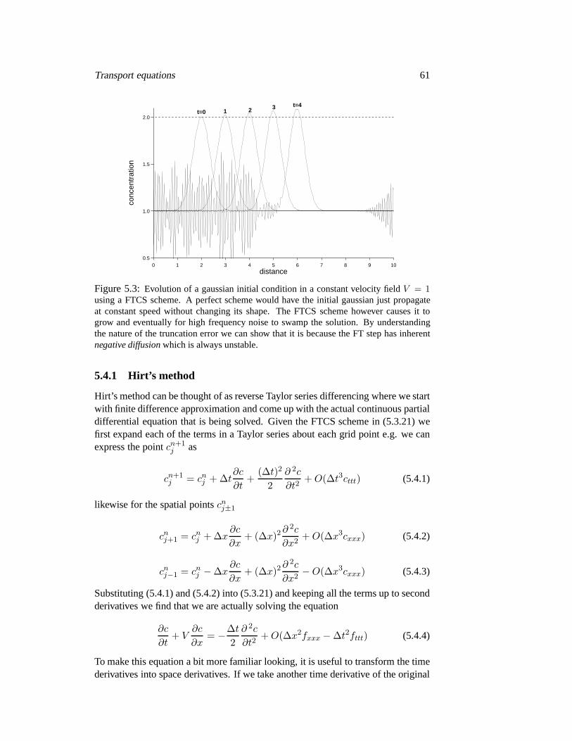
Figure 5.3:Evolution of a gaussian initial condition in a constant velocity field V = 1using a FTCS scheme. A perfect scheme would have the initial gaussian just propagateat constant speed without changing its shape. The FTCS scheme however causes it togrow and eventually for high frequency noise to swamp the solution. By understandingthe nature of the truncation error we can show that it is because the FT step has inherentnegative diffusionwhich is always unstable.

5.4.1 Hirt’s method

Hirt’s method can be thought of as reverse Taylor series differencing where we startwith finite difference approximation and come up with the actual continuous partialdifferential equation that is being solved. Given the FTCS scheme in (5.3.21) wefirst expand each of the terms in a Taylor series about each grid point e.g. we canexpress the pointcn+1

j as

cn+1j = cn

j + ∆t∂c

∂t+

(∆t)2

2

∂ 2c

∂t2+ O(∆t3cttt) (5.4.1)

likewise for the spatial pointscnj±1

cnj+1 = cn

j + ∆x∂c

∂x+ (∆x)2

∂ 2c

∂x2+ O(∆x3cxxx) (5.4.2)

cnj−1 = cn

j − ∆x∂c

∂x+ (∆x)2

∂ 2c

∂x2− O(∆x3cxxx) (5.4.3)

Substituting (5.4.1) and (5.4.2) into (5.3.21) and keepingall the terms up to secondderivatives we find that we are actually solving the equation

∂c

∂t+ V

∂c

∂x= −

∆t

2

∂ 2c

∂t2+ O(∆x2fxxx − ∆t2fttt) (5.4.4)

To make this equation a bit more familiar looking, it is useful to transform the timederivatives into space derivatives. If we take another timederivative of the original

62

equation (with constantV ) we get

∂ 2c

∂t2= −V

∂

∂x

(

∂c

∂t

)

(5.4.5)

and substituting in the original equation for∂c/∂t we get

∂ 2c

∂t2= V 2 ∂ 2c

∂x2(5.4.6)

Thus Eq. (5.4.4) becomes

∂c

∂t+ V

∂c

∂x= −

∆tV 2

2

∂ 2c

∂x2+ O(fxxx) (5.4.7)

But this is just an advection-diffusion equation with effective diffusivity κeff =−∆tV 2/2. Unfortunately, for any positive time step∆t > 0 the diffusivity is neg-ative which is a physical no-no as it means that small perturbations will gather lintwith time until they explode (see figure 5.3). This negative diffusion also accountsfor why the initial gaussian actually narrows and grows withtime. Thus the FTCSscheme is unconditionally unstable.

5.4.2 Von Neumann’s method

Von Neumann’s method also demonstrates that the FTCS schemeis effectivelyuseless, however, instead of considering the behaviour of the truncated terms wewill now consider the behaviour of small sinusoidal errors.Von Neumann stabilityanalysis is closely related to Fourier analysis (and linearstability analysis) and wewill begin by positing that the solution at any timet and pointx can be written as

c(x, t) = eσt+ikx (5.4.8)

which is a sinusoidal perturbation of wavenumberk and growth rateσ. If the realpart of σ is positive, the perturbation will grow exponentially, if it is negative itwill shrink and if it is purely imaginary, the wave will propagate (although it canbe dispersive). Now because we are dealing in discrete time and space, we canwrite t = n∆t andx = j∆x and rearrange Eq. (5.4.8) for any timestepn andgridpointj as

cnj = ζneik∆xj (5.4.9)

whereζ = eσ∆t is the amplitude of the perturbation (and can be complex). Ifζ = x+iy is complex, then we can also writeζ in polar coordinates on the complexplane asζ = reiθ wherer =

√

x2 + y2 andtan θ = y/x. Giveneσ∆t = reiθ wecan take the natural log of both sides to show that

σ∆t = log r + iθ (5.4.10)

and thus if (5.4.9) is going to remain bounded with time, it isclear that the magni-tude of the amplituder = ‖ζ‖ must be less than or equal to 1. Substituting (5.4.9)into (5.3.21) gives

ζn+1eik∆xj = ζneik∆xj −α

2ζn

(

eik∆x(j+1) − eik∆x(j−1))

(5.4.11)


or dividing by ζneik∆xj and using the identity thateikx = cos(kx) + i sin(kx),(5.4.11) becomes

ζ = 1 − iα sin k∆x (5.4.12)

Thus‖ζ‖2 = 1 + (α sin k∆x)2 (5.4.13)

Which is greater than 1 for all values ofα and k > 0 (note k = 0 meanscis constant which is always a solution but rather boring). Thus, von Neumann’smethod also shows that the FTCS method is no good for non-diffusive transportequations (it turns out that a bit of diffusion will stabilize things if it is greater thanthe intrinsic negative diffusion). So how do we come up with abetter scheme?

5.5 Usable Eulerian schemes for non-diffusive IVP’s

This section will demonstrate the behaviour and stability of several useful schemesthat are stable and accurate for non-diffusive initial value problems. While allof these schemes are an enormous improvement over FTCS (i.e.things don’t ex-plode), they each will have attendant artifacts and drawbacks (there are no blackboxes). However, by choosing a scheme that has the minimum artifacts for theproblem of interest you can usually get an effective understanding of your prob-lem. Here are a few standard schemes. . . .

5.5.1 Staggered Leapfrog

The staggered leap frog scheme uses a 2nd ordered centered difference for both thetime and space step. i.e. our simplest advection equation (5.2.2) is approximatedas

cn+1j − cn−1

j

2∆t= −V

cnj+1 − cn

j−1

2∆x(5.5.1)

or as an updating scheme

cn+1j = cn−1

j − α(cnj+1 − cn

j−1) (5.5.2)

which superficially resembles the FTCS scheme but is now a two-level schemewhere we calculate spatial differences at timen but update from timen − 1. Thuswe need to store even and odd time steps separately. Numerical Recipes gives agood graphical description of the updating scheme and showshow the even andodd grid points (and grids) are decoupled in a “checkerboard” pattern (which canlead to numerical difficulties). This pattern is where the “staggered-leapfrog” getsits name.

Using von Neumann’s method we will now investigate the stability of thisscheme. Substituting (5.4.9) into (5.5.2) and dividing byζneik∆xj we get

ζ =1

ζ− i2α sin k∆x (5.5.3)

64

or multiplying through byζ we get the quadratic equation

ζ2 + i(2α sin k∆x)ζ − 1 = 0 (5.5.4)

which has the solution that

ζ = −iα sin k∆x ±√

1 − (α sin k∆x)2 (5.5.5)

The norm ofζ now depends on the size of the Courant numberα. Since the max-imum value ofsin k∆x = 1 (which happens for the highest frequency sine wavethat can be sampled on the grid) the largest value thatα can have before the squareroot term becomes imaginary isα = 1. Thus forα ≤ 1

‖ζ‖ = 1 (5.5.6)

which says that for any value ofα ≤ 1. this scheme has no numerical diffusion(which is one of the big advantages of staggered leapfrog). For α > 1, however,the larger root ofζ is

‖ζ‖ ∼[

α +√

α2 − 1]

(5.5.7)

which is greater than 1. Therefore the stability requirement is thatα ≤ 1 or

∆t‖Vmax‖ ≤ ∆x (5.5.8)

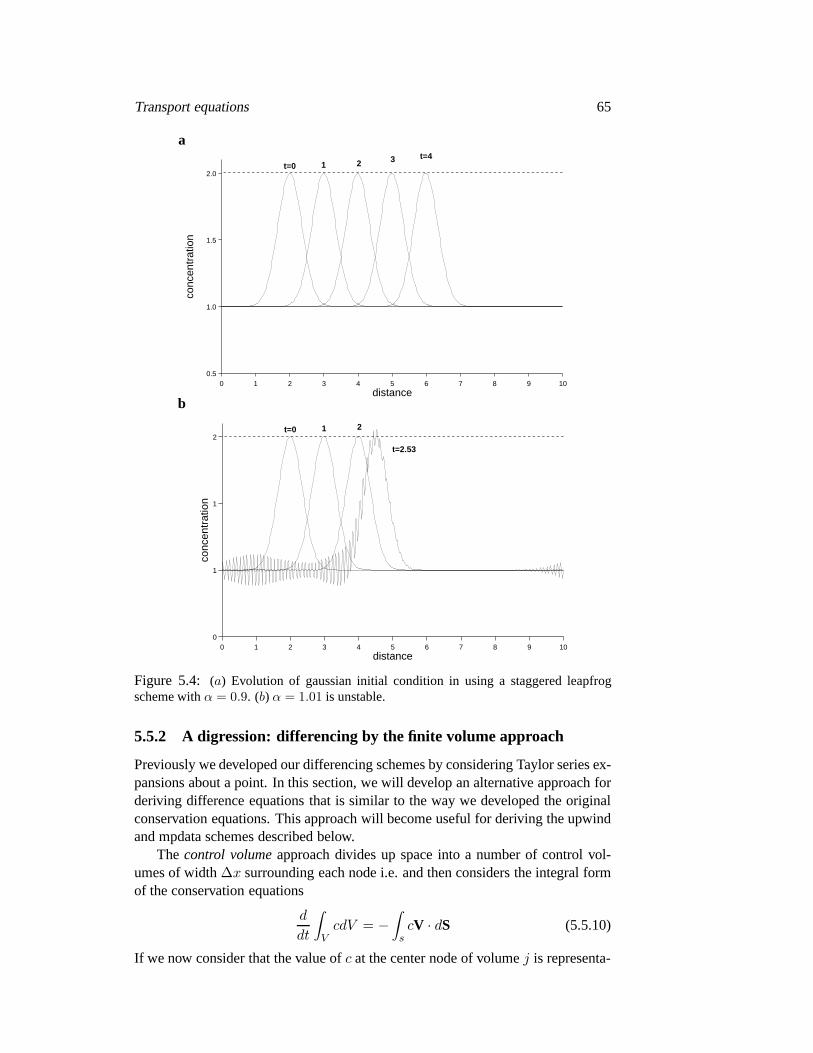
This result is known as theCourant conditionand has the physical common-senseinterpretation that if you want to maintain accuracy, any particle shouldn’t movemore than one grid point per time step. Figure 5.4 shows the behaviour of a gaus-sian initial condition forα = .9 andα = 1.01

While the staggered-leapfrog scheme is non-diffusive (like our original equa-tion) it can be dispersive at high frequencies and small values ofα. If we do aHirt’s stability analysis on this scheme we get an effectivedifferential equation

∂c

∂t+ V

∂c

∂x=

V

6

(

∆t2V 2 − ∆x2) ∂ 3c

∂x3

=V ∆x2

6

(

α2 − 1) ∂ 3c

∂x3(5.5.9)

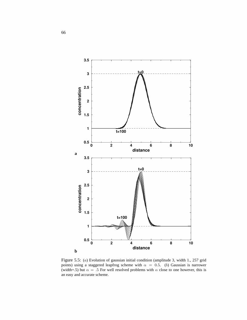
which is dispersive except whenα = 1. Unfortunately sinceα is defined for themaximum velocity in the grid, most regions usually (and should) haveα < 1. Forwell resolved features and reasonable Courant numbers, thedispersion is small.However, high frequency features and excessively small time steps can lead to morenoticeablewiggles. Figure 5.5 shows a few examples of dispersion forα = .5 andα = .5 but for a narrower gaussian. In both runs the gaussian travels around thegrid 10 times (tmax = 100) (for α = 1 you can’t tell that anything has changed).

For many problems a little bit of dispersion will not be important although thewiggles can be annoying looking on a contour plot. If howeverthe small negativevalues produced by the wiggles will feed back in dangerous ways into your solutionyou will need a non-dispersive scheme. The most commonly occuring schemes areknown asupwind schemes. Before we develop the standard upwind differencingand a iterative improvement on it, however it is useful to develop a slightly differentapproach to differencing.


a

t=0 1 2 3 t=4

0 1 2 3 4 5 6 7 8 9 10distance

0.5

1.0

1.5

2.0

conc

entr

atio

n

b

t=0 1 2

t=2.53

0 1 2 3 4 5 6 7 8 9 10distance

0

1

1

2

conc

entr

atio

n

Figure 5.4: (a) Evolution of gaussian initial condition in using a staggered leapfrogscheme withα = 0.9. (b) α = 1.01 is unstable.

5.5.2 A digression: differencing by the finite volume approach

Previously we developed our differencing schemes by considering Taylor series ex-pansions about a point. In this section, we will develop an alternative approach forderiving difference equations that is similar to the way we developed the originalconservation equations. This approach will become useful for deriving the upwindand mpdata schemes described below.

The control volumeapproach divides up space into a number of control vol-umes of width∆x surrounding each node i.e. and then considers the integral formof the conservation equations

d

dt

∫

VcdV = −

∫

scV · dS (5.5.10)

If we now consider that the value ofc at the center node of volumej is representa-

66

a

0 2 4 6 8 10

distance

0.5

1

1.5

2

2.5

3

3.5

co

nc

en

tra

tio

n

t=0

t=100

b

0 2 4 6 8 10

distance

0.5

1

1.5

2

2.5

3

3.5

co

nc

en

tra

tio

n

t=0

t=100

Figure 5.5: (a) Evolution of gaussian initial condition (amplitude 3, width 1., 257 gridpoints) using a staggered leapfrog scheme withα = 0.5. (b) Gaussian is narrower(width=.5) butα = .5 For well resolved problems withα close to one however, this isan easy and accurate scheme.


j j+1j-1

F(j-1/2) F(j+1/2)

Figure 5.6:A simple staggered grid used to define the control volume approach. Dotsdenote nodes where average values of the control volume are stored. X’s mark controlvolume boundaries at half grid points.

tive of the average value of the control volume, then we can replace the first integralby cj∆x. The second integral is the surface integral of the flux and isexactly

∫

scV · dS = cj+1/2Vj+1/2 − cj−1/2Vj−1/2 (5.5.11)

which is just the difference between the flux at the boundaries Fj+1/2 andFj−1/2.Eq. (5.5.11) is exact up to the approximations made for the values ofc andV atthe boundaries. If we assume that we can interpolate linearly between nodes thencj+1/2 = (cj+1 + cj)/2. If we use a centered time step for the time derivative thenthe flux conservative centered approximation to

∂c

∂t+

∂cV

∂z= 0 (5.5.12)

is

cn+1j − cn−1

j = −∆t

∆x

[

Vj+1/2(cj+1 + cj) − Vj−1/2(cj + cj−1)]

(5.5.13)

or if V is constant Eq. (5.5.13) reduces identically to the staggered leapfrog scheme.By using higher order interpolations for the fluxes at the boundaries additional dif-ferencing schemes are readily derived. The principal utility of this sort of differ-encing scheme is that it is automatically flux conservative as by symmetry whatleaves one box must enter the next. The following section will develop a slightlydifferent approach to choosing the fluxes by the direction oftransport.

5.5.3 Upwind Differencing (Donor Cell)

The fundamental behaviour of transport equations such as (5.5.13) is that everyparticle will travel at its own velocity independent of neighboring particles (re-member the characteristics), thus physically it might seemmore correct to say thatif the flux is moving from cellj − 1 to cell j the incoming flux should only dependon the concentrationupstream. i.e. for the fluxes shown in Fig. 5.6 theupwinddifferencingfor the flux at pointj − 1/2 should be

Fj−1/2 =

{

cj−1Vj−1/2 Vj−1/2 > 0

cjVj−1/2 Vj−1/2 < 0(5.5.14)

68

with a similar equation forFj+1/2. Thus the concentration of the incoming flux isdetermined by the concentration of thedonor celland thus the name. As a note,the donor cell selection can be coded up without anif statement by using thefollowing trick

Fj−1/2(cj−1, cj , Vj−1/2) =[

(Vj−1/2 + ‖Vj−1/2‖)cj−1 + (Vj−1/2 − ‖Vj−1/2‖)cj

]

/2

(5.5.15)or in fortran usingmax andmin as

donor(y1,y2,a)=amax1(0.,a)*y1 + amin1(0.,a)*y2f(i)=donor(x(i-1),x(i),v(i))

Simple upwind donor-cell schemes are stable as long as the Courant conditionis met. Unfortunately they are only first order schemes in∆t and∆x and thusthe truncation error is second order producing large numerical diffusion (it is thisdiffusion which stabilizes the scheme). If we do a Hirt’s style stability analysis forconstant velocities, we find that the actual equations beingsolved to second orderare

∂c

∂t+ V

∂c

∂x=

‖V ‖∆x − ∆tV 2

2

∂ 2c

∂x2(5.5.16)

or in terms of the Courant number

∂c

∂t+ V

∂c

∂x= (1 − α)

‖V ‖∆x

2

∂ 2c

∂x2(5.5.17)

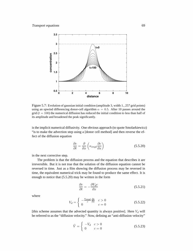
Thus as long asα < 1 this scheme will have positive diffusion and be stable.Unfortunately, any initial feature won’t last very long with this much diffusion.Figure (5.7) shows the effects of this scheme on a long run with a gaussian initialcondition. The boundary conditions for this problem are periodic (wraparound)and thus every new curve marks another pass around the grid (i.e. aftert = 10 thepeak should return to its original position). A staggered leapfrog solution of thisproblem would be almost indistinguishable from a single gaussian.

5.5.4 Improved Upwind schemes: mpdata

Donor cell methods in their simplest form are just too diffusive to be used with anyconfidence for long runs. However a useful modification of this scheme by Smo-larkiewicz [2] provides some useful corrections that remove much of the numericaldiffusion. The basic idea is that an upwind scheme (with non-constant velocities)is actual solving an advection-diffusion equation of the form

∂c

∂t+

∂V c

∂x=

∂

∂x

(

κimpl∂c

∂x

)

(5.5.18)

where

κimpl = .5(‖V ‖∆x − ∆tV 2) (5.5.19)


0 2 4 6 8 10

distance

0.5

1

1.5

2

2.5

3

3.5

co

ncen

trati

on

t=0

t=100

Figure 5.7:Evolution of gaussian initial condition (amplitude 3, width 1., 257 grid points)using an upwind differencing donor-cell algorithmα = 0.5. After 10 passes around thegrid (t = 100) the numerical diffusion has reduced the initial conditionto less than half ofits amplitude and broadened the peak significantly.

is the implicit numerical diffusivity. One obvious approach (to quote Smolarkiewicz)“is to make the advection step using a [donor cell method] andthen reverse the ef-fect of the diffusion equation

∂c

∂t=

∂

∂x

(

κimpl∂c

∂x

)

(5.5.20)

in the next corrective step.The problem is that the diffusion process and the equation that describes it are

irreversible. But it is not true that the solution of the diffusion equation cannot bereversed in time. Just as a film showing the diffusion processmay be reversed intime, the equivalent numerical trick may be found to producethe same effect. It isenough to notice that (5.5.20) may be written in the form

∂c

∂t= −

∂Vdc

∂x(5.5.21)

where

Vd =

{

−κimpl

c∂c∂x c > 0

0 c = 0(5.5.22)

[this scheme assumes that the advected quantity is always positive]. HereVd willbe referred to as the “diffusion velocity.” Now, defining an “anti-diffusion velocity”

V =

{

−Vd c > 00 c = 0

(5.5.23)

70

the reversal in time of the diffusion equation may be simulated by the advectionequation (5.5.21) with an anti-diffusion velocityV . Based on these concepts, thefollowing advection scheme is suggested. . . ”.

If we define the donor cell algorithm as

cn+1j = cn

j −[

Fj+1/2(cj , cj+1, Vj+1/2) − Fj−1/2(cj−1, cj , Vj−1/2)]

(5.5.24)

whereF is given by (5.5.15) then the mpdata algorithm is to first takea trial donor-cell step

c∗j = cnj −

[

Fj+1/2(cnj , cn

j+1, Vj+1/2) − Fj−1/2(cnj−1, c

nj , Vj−1/2)

]

(5.5.25)

then take a corrective step using the new values and the anti-diffusion velocityV ,i.e.

cn+1j = c∗j −

[

Fj+1/2(c∗

j , c∗

j+1, Vj+1/2) − Fj−1/2(c∗

j−1, c∗

j , Vj−1/2)]

(5.5.26)

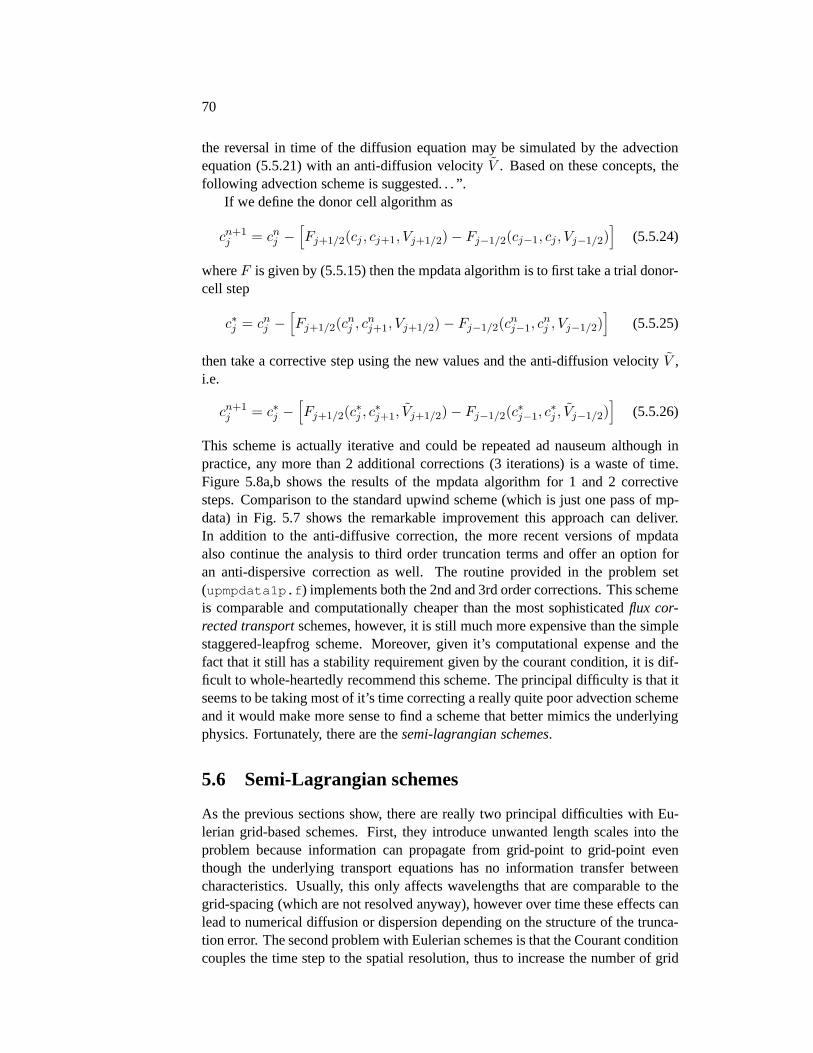
This scheme is actually iterative and could be repeated ad nauseum although inpractice, any more than 2 additional corrections (3 iterations) is a waste of time.Figure 5.8a,b shows the results of the mpdata algorithm for 1and 2 correctivesteps. Comparison to the standard upwind scheme (which is just one pass of mp-data) in Fig. 5.7 shows the remarkable improvement this approach can deliver.In addition to the anti-diffusive correction, the more recent versions of mpdataalso continue the analysis to third order truncation terms and offer an option foran anti-dispersive correction as well. The routine provided in the problem set(upmpdata1p.f) implements both the 2nd and 3rd order corrections. This schemeis comparable and computationally cheaper than the most sophisticatedflux cor-rected transportschemes, however, it is still much more expensive than the simplestaggered-leapfrog scheme. Moreover, given it’s computational expense and thefact that it still has a stability requirement given by the courant condition, it is dif-ficult to whole-heartedly recommend this scheme. The principal difficulty is that itseems to be taking most of it’s time correcting a really quitepoor advection schemeand it would make more sense to find a scheme that better mimicsthe underlyingphysics. Fortunately, there are thesemi-lagrangian schemes.

5.6 Semi-Lagrangian schemes

As the previous sections show, there are really two principal difficulties with Eu-lerian grid-based schemes. First, they introduce unwantedlength scales into theproblem because information can propagate from grid-pointto grid-point eventhough the underlying transport equations has no information transfer betweencharacteristics. Usually, this only affects wavelengths that are comparable to thegrid-spacing (which are not resolved anyway), however overtime these effects canlead to numerical diffusion or dispersion depending on the structure of the trunca-tion error. The second problem with Eulerian schemes is thatthe Courant conditioncouples the time step to the spatial resolution, thus to increase the number of grid


a0 2 4 6 8 10

distance

0.5

1

1.5

2

2.5

3

3.5

co

nc

en

tra

tio

n

t=0−100

b0 2 4 6 8 10

distance

0.5

1

1.5

2

2.5

3

3.5

co

nc

en

tra

tio

n

t=0

t=100

c0 2 4 6 8 10

distance

0.5

1

1.5

2

2.5

3

3.5

co

nc

en

tra

tio

n

t=0−100

d0 2 4 6 8 10

distance

0.5

1

1.5

2

2.5

3

3.5

co

nc

en

tra

tio

nt=0−100 (all identical)

Figure 5.8: Some schemes that actually work. Evolution of gaussian initial condition(amplitude 3, width 1., 257 total grid points) with a varietyof updating schemes. Alltimes are for a SunUltra 140e compiledf77 -fast (a) mpdata with a single upwindcorrection.α = 0.5. (0.49 cpu sec)(b) Same problem but with two corrections and a thirdorder anti-dispersion correction (1.26 s) Compare to Fig. 5.7 which is the same scheme butno corrections. Impressive eh?(c) two-level pseudo-spectral solution (α = 0.5, 256 pointiterative scheme withtol=1.e6 and 3 iterations per time step). Also not bad but deadlyslow (9.92 s). (half the grid points (3 s) also works well but has a slight phase shift) Butsave the best for last(d) A semi-lagrangian version of the same problem which is an exactsolution, has a Courant number ofα = 2 and takes only 0.05 cpu sec! (scary eh?)

points by two, increases the total run time by four because wehave to take twice asmany steps to satisfy the Courant condition. For 1-D problems, this is not really aproblem, however in 3-D, doubling the grid leads to a factor of 16 increase in time.

Clearly, in a perfect world we would have an advection schemethat is trueto the underlying particle-like physics, has no obvious Courant condition yet stillgives us regularly gridded output. Normally I would say we were crazy but theSemi-Lagrangian schemespromise just that. They are somewhat more difficultto code and they are not inherently conservative, however, for certain classes ofproblems they more than make up for it in speed and accuracy. Staniforth andCote [3] provide a useful overview of these techniques and Figure 5.9 illustratesthe basic algorithm.

Given some pointcn+1j we know that there is some particle with concentration

c at stepn that has a trajectory (or characteristic) that will pass through our grid

72

n

n+1/2

n+1

j

∆t

X

x

u(n+1,j)

c(n)

true characteristic

x

∆x

u(n+1/2)

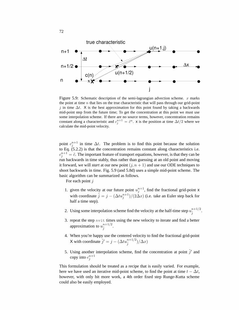
Figure 5.9: Schematic description of the semi-lagrangian advection scheme. x marksthe point at timen that lies on the true characteristic that will pass through our grid-pointj in time ∆t. X is the best approximation for this point found by taking a backwardsmid-point step from the future time; To get the concentration at this point we must usesome interpolation scheme. If there are no source terms, however, concentration remainsconstant along a characteristic andcn+1

j = cn. x is the position at time∆t/2 where wecalculate the mid-point velocity.

point cn+1j in time ∆t. The problem is to find this point because the solution

to Eq. (5.2.2) is that the concentration remains constant along characteristics i.e.cn+1j = c. The important feature of transport equations, however, isthat they can be

run backwards in time stably, thus rather than guessing at anold point and movingit forward, we will start at our new point(j, n + 1) and use our ODE techniques toshoot backwards in time. Fig. 5.9 (and 5.8d) uses a simple mid-point scheme. Thebasic algorithm can be summarized as follows.

For each pointj

1. given the velocity at our future pointun+1j , find the fractional grid-pointx

with coordinatej = j − (∆tun+1j )/(2∆x) (i.e. take an Euler step back for

half a time step).

2. Using some interpolation scheme find the velocity at the half-time stepun+1/2

j.

3. repeat the stepnvit times using the new velocity to iterate and find a betterapproximation toun+1/2

j.

4. When you’re happy use the centered velocity to find the fractional grid-pointX with coordinatej′ = j − (∆tu

n+1/2

j)/∆x)

5. Using another interpolation scheme, find the concentration at pointj′ andcopy intocn+1

j

This formulation should be treated as a recipe that is easilyvaried. For example,here we have used an iterative mid-point scheme, to find the point at timet − ∆t,however, with only bit more work, a 4th order fixed step Runge-Kutta schemecould also be easily employed.


An example of this algorithm in Matlab using a mid-point scheme with firstorder interpolation for velocity and cubic interpolation for the values can be written

it=1; % iteration counter (toggles between 1 and 2)nit=2; % next iteration counter (toggles between 2 and 1)for n=1:nstept=dt*n; % set the timevm=.5*(v(:,it)+v(:,nit)); % find mean velocity at mid timevi=v(:,nit); % set initial velocity to the future velocity on the grid pointsfor k=1:kit

xp=x-.5*dt*vi; % get new pointsxp=makeperiodic(xp,xmin,xmax); % patch up boundary conditionsvi=interp1(x,vm,xp,’linear’); % find centered velocities at mid-time

endxp=x-dt*vi; % get points at minus a whole step;xp=makeperiodic(xp,xmin,xmax); % patch up boundary conditionsc(:,nit)=interp1(x,c(:,it),xp,’cubic’); % use cubic interpolation to get the new point

end

The functionmakeperiodic implements the periodic boundary conditionsby simply mapping points that extend beyond the domainxmin ≤ x ≤ xmax backinto the domain. Other boundary conditions are easily implemented in 1-D.

These matlab routines demonstrate the algorithm rather cleanly, and make con-siderable use of the object oriented nature of Matlab. Unfortunately, Matlab isnowhere near as efficient in performance as a compiled language such as fortran.Moreover, if there are many fields that require interpolation, it is often more sensi-ble to calculate the weights separately and update the function point-by-point. Thefollowing routines implement the same problem but in f77.

The following subroutines implement this scheme for a problem where thevelocities are constant in time. This algorithm uses linearinterpolation for the ve-locities at the half times and cubic polynomial interpolation for the concentrationat time stepn. This version does cheat a little in that it only calculates the inter-polating coefficients once during the run in subroutinecalcintrp. But this is asmart thing to do if the velocities do not change with time. The results are shownin Fig. 5.8d for constant velocity. For any integer value of the courant condition,this scheme is a perfect scroller. Fig. 5.8d has a courant number of 2, thus everytime step shifts the solution around the grid by 2 grid points.

c***********************************************************************c upsemlag1: 1-D semi-lagrangian updating scheme for updating anc array without a source term. Uses cubic interpolation for the initialc value at time -\Delta t Assumes that all the interpolationc weightings have been precomputed using calcintrp1d01 (whichc calls getweights1d01 in semlagsubs1d.f)c arguments arec arn(ni): real array for new valuesc aro(ni): real array of old valuesc ni: full array dimensionsc wta : array of nterpolation weights for bicubic interpolation atc the n-1 step, precalculated in calcintrp1d01c ina : array of coordinates for interpolating 4 points at the n-1c step precalculated in calcintrp1d01c is,ie: bounds of domain for updatingc***********************************************************************

subroutine upsemlag1(arn,aro,wta,ina,ni,is,ie)

74

implicit noneinteger ni,i,is,iereal arn(ni),aro(ni),wta(4,ni)integer ina(4,ni)

do i=is,ie ! cubic interpolationarn(i)=(wta(1,i)*aro(ina(1,i))+wta(2,i)*aro(ina(2,i))+

& wta(3,i)*aro(ina(3,i))+wta(4,i)*aro(ina(4,i)))enddoreturnend

c***********************************************************************c calcintrp1d01 routine for calculating interpolation points andc coefficients for use in semi-lagrangian schemes.c does linear interpolation of velocities and cubicc interpolation for end points for use with upsemlag1cc Version 01: just calls getweights1d01 where all the heavyc lifting is donec arguments arec ni: full array dimensionsc u(ni): gridded velocityc wta :array of interpolation weights for cubic interpolation at n-1 time pointc ina: array of coordinates for interpolating 4 points at the n-1 stepc is,ie bounds of domain for updatingc dtdz: dt/dz time step divided by space step (u*dt/dz) isc grid points per time stepc it: number of iterations to try to find best mid-point velocityc***********************************************************************

subroutine calcintrp1d01(wta,ina,u,ni,is,ie,dtdz,it)implicit nonereal hlf,sxtparameter(hlf=.5, sxt=0.1666666666666666667d0)integer ni,i,is,iereal u(ni) ! velocity arrayreal wta(4,ni)real dtdz,hdtinteger ina(4,ni)integer it

hdt =.5*dtdz

do i=is,iecall getweights1d01(u,wta(1,i),ina(1,i),ni,i,hdt,it)

enddoreturnend

include ’semilagsubs1d.f’

and all the real work is done in the subroutinegetweights1d01

c***********************************************************************c Semilagsubs1d: Basic set of subroutines for doing semilangrangianc updating schemes in 1-D. At the the moment there are only 2c routines:c getweigths1d01: finds interpolating weigths and arrayc indices given a velocity field and a starting index ic version 01 assumes periodic wrap-around boundariesc cinterp1d: uses the weights and indices to return thec interpolated value of any arraycc Thus a simple algorithm for semilagrangian updating might look likec do i=is,iec call getweights1d01(wk,wt,in,ni,i,hdtdx,it)c arp(i)=cinterp1d(arn,wt,in,ni)c enddoc***********************************************************************

c***********************************************************************


c getweights1d01 routine for calculating interpolation points andc coefficients for use in semi-lagrangian schemes.c does linear interpolation of velocities and cubicc interpolation for end points for use with upsemlag2cc Version 01 calculates full interpolating index and assumesc periodic wraparound boundariescc arguments arec ni: full array dimensionsc u(ni): gridded velocityc wt : interpolation weights for bicubic interpolation at the n-1 stepc in: indices for interpolating 4 points at the n-1 stepc is,ie bounds of domain for updatingc dtdz: dt/dz time step divided by space step (u*dt/dz) isc grid points per time stepc it: number of iterations to try to find best mid-point velocityc***********************************************************************

subroutine getweights1d01(u,wt,in,ni,i,hdt,it)parameter(hlf=.5, sxt=0.1666666666666666667d0)implicit noneinteger ni,ireal wt(4),ri,di,u(ni),ui,sreal hdtreal t(4) ! offsetsinteger in(4),k,it,i0,ipui(s,i,ip)=(1.-s)*u(i)+s*u(ip) ! linear interpolation pseudo-func

di=hdt*u(i) ! calculate length of trajectory to half-time stepdo k=1,it !iterate to get gridpoint at half-time step

ri=i-diif (ri.lt.1) then ! fix up periodic boundaries

ri=ri+ni-1elseif (ri.gt.ni) then

ri=ri-ni+1endifi0=int(ri) ! i0 is lower interpolating indexs=ri-i0 !s is difference between ri and i0di=hdt*ui(s,i0,i0+1) !recalculate half trajectory length

enddori=i-2.*di-1. !calculate real position at full time stepif (ri.lt.1) then ! fix up periodic boundaries again

ri=ri+ni-1elseif (ri.gt.ni) then

ri=ri-ni+1endifin(1)=int(ri) !set interpolation indicesdo k=2,4

in(k)=in(k-1)+1enddoif (in(1).gt.ni-3) then

do k=2,4 ! should only have to clean up k=2,4if (in(k).gt.ni) in(k)=in(k)-ni+1

enddoendift(1)=ri+1.-float(in(1)) !calculate weighted distance from each interpolating pointdo k=2,4

t(k)=t(k-1)-1.enddowt(1)= -sxt*t(2)*t(3)*t(4) ! calculate interpolating coefficients for cubic interpolationwt(2)= hlf*t(1)*t(3)*t(4)wt(3)=-hlf*t(1)*t(2)*t(4)wt(4)= sxt*t(1)*t(2)*t(3)returnend

c***********************************************************************c cinterp1d: do cubic interpolation on an array given a set ofc weights and indicesc***********************************************************************

76

real function cinterp1d(ar,wt,in,ni)implicit noneinteger nireal ar(ni)real wt(4)integer in(4)

cinterp1d=(wt(1)*ar(in(1))+wt(2)*ar(in(2))+ ! cubic interpolation& wt(3)*ar(in(3))+wt(4)*ar(in(4)))returnend

For more interesting problems where the velocities change with time, you willneed to recalculate the weights every time step. This can be costly but the overallaccuracy and lack of courant condition still makes this my favourite scheme. Here’sanother version of the code which uses function calls to find the weights and do theinterpolation2.

c***********************************************************************c upsemlag2: 1-D semi-lagrangian updating scheme for updating anc array without a source term. Uses cubic interpolation for thec initial value at time -\Delta t.cc Version 2 assumes velocities are known but changing with time andc uses function calls for finding weights and interpolating. A goodc compiler should inline these calls in the loopcc Variables:c arn(ni): real array of old values (n)c arp(ni): real array for new values (n+1)c vn(ni): velocities at time nc vp(ni): velocities at time n+1c wk(ni): array to hold the average velocity .5*(vn+vp)c ni: full array dimensionsc dx: horizontal grid spacingc dt: time stepc is,ie: bounds of domain for updatingc it: number of iterations to find interpolating pointc***********************************************************************

subroutine upsemlag2(arn,arp,vn,vp,wk,ni,is,ie,dx,dt,it)implicit noneinteger ni,i,is,iereal arp(ni),arn(ni)real vp(ni),vn(ni)real wk(ni)real dx,dtinteger it

real hdt,hdtdxreal wt(4),in(4) ! weights and indices for interpolationreal cinterp1dexternal cinterp1d

hdt=.5*dthdtdx=hdt/dx

call arrav3(wk,vn,vp,ni) ! get velocity at mid level

do i=is,iecall getweights1d01(wk,wt,in,ni,i,hdtdx,it)arp(i)=cinterp1d(arn,wt,in,ni)

enddo

2note: a good compiler will inline the subroutine calls for you if you include the subroutines inthe file. On Suns running Solaris an appropriate option wouldbeFFLAGS=-fast -O4, look atthe man pages for more options


returnend

include ’semilagsubs1d.f’

Using this code, the run shown in Figure 5.8d is about 10 timesslower (0.5seconds) but the courant condition can easily be increased with no loss of accuracy.Moreover, it is still about 50 times faster than the matlab script (as fast as computersare getting, a factor of 50 in speed is still nothing to sneezeat).

5.6.1 Adding source terms

The previous problem of advection in a constant velocity field is a cute demonstra-tion of the semi-lagrangian schemes but is a bit artificial because we already knowthe answer (which is to exactly scroll the solution around the grid). More interest-ing problems arise when there is a source term, i.e. we need tosolve equations ofthe form

∂c

∂t+ V

∂c

∂x= G(x, t) (5.6.1)

However, if we remember that the particle approach to solving this is to solve

Dc

Dt= G(x, t) (5.6.2)

i.e. we simply have to integrateG along the characteristic. Again we can use someof the simple ODE integrator techniques. For a three-level,second order schemewe could just use a mid point step and let

cn+1j = cn−1

j′+ ∆tG(j, n) (5.6.3)

alternatively it is quite common forG to have a form likecg(x) and it is somewhatmore stable to use a trapezoidal integration rule such that,for a two-level scheme

cn+1j = cn

j′+

∆t

2

[

(cg)nj′

+ (cg)n+1j )

]

(5.6.4)

or re-arranging

cn+1j = cn

j′

1 + βgn−1j′

1 − βgn+1j

(5.6.5)

whereβ = ∆t/2. Figure 5.6.1 shows a solution of Eq. (5.6.5) for a problem withnon-constant velocity i.e.

∂c

∂t+ V

∂c

∂x= −c

∂V

∂x(5.6.6)

and compares the solutions for staggered-leapfrog, mpdataand a pseudo-spectraltechnique (next section). Using a Courant number of 10 (!) this scheme is two-orders of magnitude faster and has fewer artifacts than the best mpdata scheme.

78

0 10 20 30

distance

0

1

2

3

concentr

ation

0

1

2

3

concentr

ation

0 10 20 30

distance

0

1

2

3

0

1

2

3

staggered−leapfrog mpdata (ncor=3, i3rd=1)

semi−lagrangian pseudo−spectral

t=0

90

15

105

30 4560

75120

t=0

12090 15 105 30 4560 75

0.09s 1.32s

0.02s 15.85s

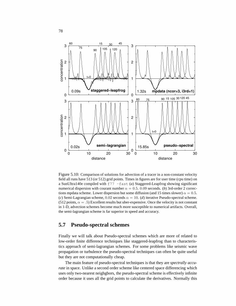
Figure 5.10:Comparison of solutions for advection of a tracer in a non-constant velocityfield all runs have 513 (or 512) grid points. Times in figures are for user time (cpu time) ona SunUltra140e compiled withf77 -fast (a) Staggered-Leapfrog showing significantnumerical dispersion with courant numberα = 0.5. 0.09 seconds. (b) 3rd-order 2 correc-tions mpdata scheme. Lower dispersion but some diffusion (and 15 times slower)α = 0.5.(c) Semi-Lagrangian scheme,0.02 secondsα = 10. (d) iterative Pseudo-spectral scheme.(512 points,α = .5) Excellent results but uber-expensive. Once the velocity is not constantin 1-D, advection schemes become much more susceptible to numerical artifacts. Overall,the semi-lagrangian scheme is far superior in speed and accuracy.

5.7 Pseudo-spectral schemes

Finally we will talk about Pseudo-spectral schemes which are more of related tolow-order finite difference techniques like staggered-leapfrog than to characteris-tics approach of semi-lagrangian schemes. For some problems like seismic wavepropagation or turbulence the pseudo-spectral techniquescan often be quite usefulbut they are not computationally cheap.

The main feature of pseudo-spectral techniques is that theyarespectrally accu-rate in space. Unlike a second order scheme like centered space differencing whichuses only two-nearest neighgbors, the pseudo-spectral scheme is effectively infiniteorder because it uses all the grid points to calculate the derivatives. Normally this


would be extremely expensive because you would have to doN operations witha stencil that isN points wide. However, PS schemes use a trick owing to FastFourier Transforms that can do the problem in orderN log2 N operations (that’swhy they call them fast).

The basic trick is to note that the discrete Fourier transform of an evenly spacedarray ofN numbershj (j = 0 . . . N − 1) is

Hn = ∆N−1∑

j=0

hjeiknxj (5.7.1)

where∆ is the grid spacing and

kn = 2πn

N∆(5.7.2)

is the wave number for frequencyn. xj = j∆ is just the position of pointhj .The useful part of the discrete Fourier Transform is that it is invertable by a similaralgorithm, i.e.

hj =1

N

N−1∑

n=0

Hne−iknxj (5.7.3)

Moreover, with the magic of theFast Fourier Transformor FFT, all these sums canbe done inN log2 N operations rather than the more obviousN2 (see numericalrecipes). Unfortunately to get that speed with simple FFT’s(like those found inNumerical Recipes [4] requires us to have grids that are onlypowers of 2 pointslong (i.e.2, 4, 8, 16, 32, 64 . . .). More general FFT’s are available but ugly to code;however, a particularly efficient package of FFT’s that can tune themselves to yourplatform and problem can be found in the FFTW3 package.

Anyway, you may ask how this is going to help us get high order approxima-tions for ∂h/∂x? Well if we simply take the derivative with respect tox of Eq.(5.7.3) we get

∂hj

∂x=

1

N

N−1∑

n=0

−iknHne−iknxj (5.7.4)

but that’s just the inverser Fourier Transform of−iknHn which we can write asF−1[−iknHn] whereHn = F [hj ]. Therefore the basic pseudo-spectral approachto spatial differencing is to use

∂cj

∂x= F−1[−iknF [cj ]] (5.7.5)

i.e. transform your array into the frequency domain, multiply by −ikn and thentransform back and you will have a full array of derivatives that useglobal infor-mation about your array.

In Matlab, such a routine looks like

function [dydx] = psdx(y,dx)% psdx - given an array y, with grid-spacing dx, calculate dydx using fast-fourier transforms

3Fastest Fourier Transform in the West

80

ni=length(y);kn=2.*pi/ni/dx; % 1/ni times the Nyquist frequencyik=i*kn*[0:ni/2 -(ni/2)+1:-1]’; % calculate ikdydx=real(ifft(ik.*fft(y))); % pseudo-spectral first derivativereturn;

In f77, a subroutine might look something like

c**************************************************************************c psdx01: subroutine to calculate df/dx = F^{-1} [ ik F[f]] usingc pseudo-spectral techniques. here F is a radix 2 FFT and k is thec wave number.c routines should work in place, ie on entrance ar=f and onc exit ar=df/dx. ar is complex(ish)c**************************************************************************

subroutine psdx01(ar,ni,dx)implicit noneinteger nireal ar(2,ni),dx

integer ndouble precision k,pi,kn,tmpreal inidata pi /3.14159265358979323846/ini=1./nikn=2.*pi*ini/dx

call four1(ar,ni,1) ! do forward fourier transformdo n=1,ni/2+1 !for positive frequncies multiply by ik

k=kn*(n-1)tmp=-k*ar(1,n)ar(1,n)=k*ar(2,n)ar(2,n)=tmp

enddodo n=ni/2+2,ni !for negative frequncies

k=kn*(n-ni-1)tmp=-k*ar(1,n)ar(1,n)=k*ar(2,n)ar(2,n)=tmp

enddocall four1(ar,ni,-1)call arrmult(ar,2*ni,ini)returnend

Note that the array is assumed to be complex and of a length that is a power of2 so that it can use the simplest FFT from Numerical recipesfour1.

5.7.1 Time Stepping

Okay, that takes care of the spatial derivatives but we stillhave to march throughtime. The Pseudo part of the Pseudo-Spectral methods is justto use standard finitedifferences to do the time marching and there’s the rub. If weremember fromour stability analysis, the feature that made the FTCS scheme explode was not thehigh-order spatial differencing but the low order time-differencing. So we mightexpect that a FTPS scheme like

cn+1j = cn

j − ∆tPSx [cV ]n (5.7.6)

is unstable (and it is). NotePSx [cV ]n is the Pseudo-spectral approximation to∂cV /∂x at time stepn. One solution is to just use a staggered-leapfrog stepper


(which works but has a stability criterion ofα < 1/π and still is dispersive) or I’vebeen playing about recently with some two-levelpredictor-correctorstyle updateschemes that use

cn+1j = cn

j −∆t

2

(

PSx [cV ]n + PSx [cV ]n+1)

(5.7.7)

which is related to a 2nd order Runge-Kutta scheme and uses the average of thecurrent time and the future time. The only problem with this scheme is that youdon’t know (cV )n+1 ahead of time. The basic trick is to start with a guess that(cV )n+1 = (cV )n which makes Eq. (5.7.7) a FTPS scheme, but then use the newversion ofcn+1 to correct for the scheme. Iterate until golden brown.

A snippet of code that implements this is

do n=1,nstepst=dt*n ! calculate timenn=mod(n-1,2)+1 !set pointer for step nnnp=mod(n,2) +1 !set pointer for step n+1gnn=gp(nn) ! starting index of grid ngnp=gp(nnp) ! starting index of grid n+1tit=1resav=1.do while (resav.gt.tol)

if (tit.eq.1) call arrcopy(ar(gnp),ar(gnn),npnts)call uppseudos01(ar(gnn),ar(gnp),wp(gnn),wp(gnp),dar,npnts

& ,dt,dx,resav) !update using pseudo-spec techniquetit=tit+1

enddoenddo ! end the loop

and the pseudo-spectral scheme that does a single time step is

c**************************************************************************c uppseudos01: subroutine to do one centered time update usingc spatial derivatives calculated by pseudo-spectral operatorsc updating scheme isc ddx=d/dx( .5*(arn*wn+arp*wp)c arp=arn+dt*ddxc returns L2 norm of residual for time stepc**************************************************************************

subroutine uppseudos01(arn,arp,wn,wp,ddx,npnts,dt,dx,resav)implicit noneinteger npnts !number of 1d grid pointsreal arn(npnts),arp(npnts) ! array at time n and n+1real wn(npnts),wp(npnts) ! velocity at time n and n+1real ddx(2,npnts) ! complex array for holding derivativesreal dt,dxreal res,resav,ressum

integer nreal ap

do n=1,npnts ! load real component of ddx (and zero im)ddx(1,n)=.5*(arn(n)*wn(n)+arp(n)*wp(n))ddx(2,n)=0.

enddo

call psdx01(ddx,npnts,dx) ! use pseudo spectral techniques to! calculate derivative

ressum=0.do n=1,npnts ! update arp at time n+1 and calculate residual

ap=arn(n)-dt*ddx(1,n)res=ap-arp(n)ressum=ressum+res*res

82

arp(n)=apenddoresav=sqrt(ressum)/npntsreturnend

The various figures using pseudo-spectral schemes in this chapter use this al-gorithm. For problems with rapidly changing velocities it seems quite good but itis extremely expensive and it seems somewhat backwards to spend all the energyon getting extremely good spatial derivatives when all the error is introduced inthe time derivatives. Most unfortunately, these schemes are still tied to a courantcondition and it is usually difficult to implement boundary conditions. Still somepeople love them. C’est La Guerre.

0 10 20 30

distance

0

1

2

3

co

nce

ntr

atio

n

semi−lagrangian (1024 pts, α=20, t=0.05s)

pseudo−spectral (256 pts,α=0.5,t=4.98s)

Figure 5.11: Comparison of non-constant velocity advection schemes for Semi-Lagrangian scheme with 1025 points and a Pseudo-Spectral scheme at 256 points.The two schemes are about comparable in accuracy but the semi-lagrangian schemeis nearly 100 times faster.

5.8 Summary

Pure advective problems are perhaps the most difficult problems to solve numeri-cally (at least with Eulerian grid based schemes). The fundamental physics is thatany initial condition just behaves as a discrete set of particles that trace out theirown trajectories in space and time. If the problems can be solved analytically bycharacteristics then do it. If the particles can be tracked as a system of ODE’sthat’s probably the second most accurate approach. For gridbased methods thesemi-lagrangian hybrid schemes seem to have the most promise for real advectionproblems. While they are somewhat complicated to code and are not conservative,


they are more faithful to the underlying characteristics than Eulerian schemes, andthe lack of a courant condition makes them highly attractivefor high-resolutionproblems. If you just need to get going though, a second orderstaggered leapfrogis the simplest first approach to try. If the numerical dispersion becomes annoyinga more expensive mpdata scheme might be used but they are really superseded bythe SL schemes. In all cases beware of simple upwind differences if numericaldiffusion is not desired.

Bibliography

[1] B. P. Leonard. A survey of finite differences of opinion onnumerical muddlingof the incomprehensible defective confusion equation, in:T. J. R. Hughes, ed.,Finite element methods for convection dominated flows, vol.34, pp. 1–17,Amer. Soc. Mech. Engrs. (ASME), 1979.

[2] P. K. Smolarkiewicz. A simple positive definite advection scheme with smallimplicit diffusion, Mon Weather Rev 111, 479–486, 1983.

[3] A. Staniforth and J. Cote. Semi-Lagrangian integrationschemes for atmo-spheric models—A review, Mont. Weather Rev. 119, 2206–2223, Sep 1991.

[4] W. H. Press, B. P. Flannery, S. A. Teukolsky and W. T. Vetterling. NumericalRecipes, Cambridge Univ. Press, New York, 2nd edn., 1992.

Documents

Transport: Non-diffusive, flux conservative initial value problems and