Transport infrastructure, intraregional

trade, and economic growth

A study of South America

Master‟s thesis within Economics

Author: Anneloes Muuse

Tutor: Johan Klaesson

Hanna Larsson

Jönköping May 2010

Master‟s Thesis in Economics

Title: Transport infrastructure, intraregional trade, and economic growth: A

study of South America

Author: Anneloes Muuse

Tutor: Johan Klaesson

Hanna Larsson

Date: 2010-05-27

Subject terms: Granger causality, gravity equation, intraregional trade, South America, transport infrastructure

Abstract

In October 2000 the Initiative for the Integration of Regional Infrastructure in

South America (IIRSA) was launched. The purpose of the IIRSA is to improve

integration of the South American countries and intraregional trade between them.

One of the ultimate goals is to promote sustainable growth. The purpose of this

paper is to find out if a better quantity and quality of transport infrastructure

increases intraregional trade in South America. It is found that the quantity of

transport infrastructure increases intraregional trade. On the other hand, there is no

evidence for the quality of transport infrastructure increasing intraregional trade in

South America. Furthermore, this paper investigates whether economic growth

can be obtained through more trade. In other words, this paper examines if trade

causes growth. The results do not confirm the trade-growth causality for all

countries. The difference between the existence of a trade-growth causal

relationship or not could be explained by the core commodities that the different South American countries export.

1

Table of Contents

1 Introduction .................................................................................... 3

2 Background .................................................................................... 6

2.1 Literature review .................................................................................... 6

2.1.1 Infrastructure, productivity, and economic growth ...................... 6

2.1.2 Infrastructure and trade ............................................................... 7

2.1.3 International trade and economic growth ..................................... 7

2.1.4 Infrastructure, trade, and economic growth in South America ..... 9

2.2 Trade theory ......................................................................................... 10

2.2.1 Neoclassical trade theory .......................................................... 10

2.2.2 New trade theory ....................................................................... 11

2.2.3 Trade theory and geographical economics ................................. 13

2.2.4 The gravity model ..................................................................... 14

3 Methodology ..................................................................................16

3.1 Model estimation .................................................................................. 16

3.1.1 Panel data ................................................................................. 16

3.1.2 Fixed effects an random effects ................................................. 17

3.2 A gravity model with transport infrastructure ....................................... 17

3.2.1 The dependent variable ............................................................. 18

3.2.2 Explanatory variables ................................................................ 18

3.2.3 Dummy variables ...................................................................... 19

3.2.4 Data collection .......................................................................... 20

4 Statistical methods.........................................................................21

4.1 Descriptive statistics ............................................................................. 21

4.2 Collinearity and multicollinearity ......................................................... 22

4.3 Hausman test ........................................................................................ 22

4.4 Heteroskedasticity ................................................................................ 23

4.5 Autocorrelation .................................................................................... 23

5 Results ............................................................................................24

6 Granger causality tests ..................................................................26

6.1 Statistical methods................................................................................ 26

6.2 Results of the Granger causality tests.................................................... 26

7 Conclusion .....................................................................................29

References ............................................................................................31

Appendix ..............................................................................................35

2

Boxes

Box 1 – A standard gravity equation ....................................................................... 14

Box 2 – A gravity equation with road infrastructure ................................................ 17

Tables

Table 1 – Descriptive statistics ............................................................................... 21

Table 2 – Auxiliary regression results for multicollinearity ..................................... 22

Table 3 – Results for the regression of the gravity model ........................................ 24

Table 4 – Granger causality results ......................................................................... 27

Appendix

Appendix 1 – Correlation matrix ............................................................................ 35

Appendix 2 – Hausman test for fixed- and random effects ...................................... 36

Appendix 3 – Modified Wald test for groupwise heteroskedasticity ........................ 36

Appendix 4 – Wooldridge test for autocorrelation in panel data .............................. 36

Appendix 5 – Augmented Dickey-Fuller test .......................................................... 36

Appendix 6 – Non-stationary intraregional trade data: Argentina ............................ 37

Appendix 7 – Stationary intraregional trade data: Argentina ................................... 37

3

1 Introduction

In October 2000 the Initiative for the Integration of Regional Infrastructure in South

America (IIRSA) was launched by the 12 countries in South America: Argentina, Bolivia,

Brazil, Chile, Colombia, Ecuador, Guyana, Paraguay, Peru, Suriname, Uruguay, and

Venezuela. The purpose of the IIRSA is to improve integration of the South American

countries and intraregional trade between them (Mesquita-Moreira, 2008). The Andean

Community of Nations (CAN)1 and the Southern Common Market (MERCOSUR)

2

agreements have brought more integration in South America already; however the area is

still lagging behind other parts of the world (e.g. Asia and Europe) in terms of intraregional

trade. This can be explained, first of all, by the fact that the free trade zones are still

imperfect, and secondly by the bad quality and quantity of transport infrastructure. The

IIRSA was created because the governments of the 12 South American countries thought

that improvement in integration, which in turn would improve intraregional trade, could

come from improving transport infrastructure in and between the countries rather than from

further developing free trade areas.

Infrastructure has always been a major impediment to South America:

“Cross-country rivalries or animosities and fear of invasion by neighboring countries

discouraged the development of infrastructure that could link, rather than separate, different

countries and could expand markets beyond national borders. Thus, little cross-country-

infrastructure was built. For this reason, trade among Latin American countries developed

much less than it could have developed and certainly less than trade between these countries

and the rest of the world. The links with the rest of the world were mostly Europe and the

United States rather than with other Latin American countries and used sea routes, and

more recently, planes.” (Tanzi, 2005 p.5)

Besides these historical reasons for the inappropriate infrastructure in South America, there

are also the natural physical barriers hampering the infrastructure development. Nowadays,

infrastructure development is perceived as a source for competitiveness and governments

want to invest in infrastructure. Priority is especially to update the road system to increase

intraregional trade. (Acosta Rojas, Calfat, & Flôris Jr, 2005)

Many researchers have recognized that poor infrastructure is a barrier to trade. A survey

from the World Bank (2004) shows that Latin America scores highest on businesses that

consider infrastructure as a serious problem. However, very little research has addressed the

effect of infrastructure on trade in South America. Especially intraregional trade has been

1 In 2010 CAN includes the following countries: Bolivia, Colombia, Ecuador, and Peru. Furthermore,

Argentina, Brazil, Chile, Paraguay, and Uruguay are associate members.

2 In 2010 MERCOSUR includes the following countries: Argentina, Brazil, Paraguay, Uruguay, and

Venezuela. Thereby, Bolivia, Chile, Colombia, Ecuador, and Peru are associate members.

4

looked upon by only few. Therefore, this paper will try to fill this gap of research, and focus

on the research question:

“How does transport infrastructure affect intraregional trade in South America?”3

In this paper the focus will be on road infrastructure. Road infrastructure is the most

frequently used way of transport for intraregional trade in South America (Acosta Rojas et

al., 2005)

In studying this question, there will be distinguished between the quantity and quality of

road infrastructure. Following this, the following hypotheses are made:

H1: The quantity of road infrastructure positively influences intraregional trade in South

America.

H2: The quality of road infrastructure positively influences intraregional trade in South

America.

One of the IIRSA‟s ultimate goals is to promote sustainable growth. It is, therefore,

interesting to find out whether sustainable growth can be obtained through higher amounts

of trade, in particular intraregional trade. In other words, it is interesting to find out the

relation between trade and economic growth. Therefore, a second research question will be:

“What is the relation between trade and economic growth in South America?”

From this question, and especially looking at intraregional trade, the hypothesis follows:

H3: Intraregional trade causes economic growth

No one else has looked at the influence of infrastructure on intraregional trade in South

America before. Furthermore, a congestion variable to measure the quality of infrastructure

is introduced in this paper. None of the previous studies concerning infrastructure and trade

have measured quality of infrastructure in this way. With these novelties, this paper

contributes to the literature on infrastructure and trade.

The first sub-question will be tried to be answered using panel data of the 12 South

American countries for the years 1993-1999. A gravity model will then be used to examine

the influence of several infrastructure indicators on intraregional trade. The second sub-

question will be studied using time-series data of the 12 South American countries for the

years 1962-2008. With Granger causality tests, the relation between trade and economic

growth will be evaluated. In this way, this study tries to find out whether the IIRSA project

will indeed help to improve the economic position of South America.

3 Intraregional trade is defined by trade within the South American region, i.e. trade between Argentina,

Bolivia, Brazil, Chile, Colombia, Ecuador, Guyana, Paraguay, Peru, Suriname, Uruguay, and Venezuela.

5

The outline of the paper is as follows. Section 2 will deal with previous literature on the

topic of this paper. Moreover, this section will also discuss some general trade theories and

link it to theories of geographical economics. Next, in section 3 the methodology is

discussed starting with some remarks on the kind of data and model that will be used. After

that the model itself will be explained on the hand of the different variables that are

included. In section 4, the statistical methods necessary to obtain the right model are

explained. Accordingly, the results of the model will be presented and discussed in section

5. Section 6 will then shortly discuss the relation between trade and economic growth on the

hand of Granger causality tests. Finally, section 7 presents the conclusion of this research

and some suggestions for further research will be given.

6

2 Background

2.1 Literature review

In the last few decades quite some literature has been dedicated to the role of infrastructure

in the economy. This started with studies on the role of infrastructure on economic growth,

and later the role of infrastructure in international trade was widely discussed. Furthermore,

the relation between trade and economic growth got the attention of many studies. An

overview of the most important literature on these topics is given in the next four

subsections.

2.1.1 Infrastructure, productivity, economic growth, and costs

There is great consensus that infrastructure, such as transport, telecommunication, and

power, are of great essence to economic activity (World Bank, 2004). The quality and

extensiveness of infrastructure networks significantly impact economic growth (World

Economic Forum, 2009). Gramlich (1994) mentions that despite the importance of

infrastructure, economists paid little attention to this factor until the late 1980s. The first

literature on the influence of infrastructure on economic growth comes from Aschauer

(1989). He argues that the „core‟ infrastructure should possess great explanatory power for

productivity. The same result was found by Munnell (1990), Holtz-Eakin (1994), Lynde &

Richmond (1993), and many others. In a study about public investment spending and

productivity in the United Kingdom, Lynde & Richmond (1993) conclude that higher

infrastructure investments could have brought about an increase in labor productivity in the

United Kingdom of about 4 to 4,5% per year. The former studies all found a very large

effect of infrastructure on economic growth. On the other hand, there are also many studies

that did not find such a large impact of infrastructure. For instance,(Nadiri & Mamuneas

(1994) find that the magnitude of the effects of infrastructure on productivity is not as large

as suggested in the studies of Aschauer (1989) and many others. Similarly, Holtz-Eakin &

Schwartz (1994), who were among the first to incorporate infrastructure in a neoclassical

growth model, do not find a very large role for infrastructure in the growth pattern of states.

However, they also say that the importance of infrastructure is probably underestimated as

they cannot totally control for the endogeneity problem, that is higher productivity gives

states more money to invest in infrastructure. Building on the work of Mankiw, Romer, &

Weil (1992) concerning the Solow-Swan growth model, Knight, Loayza, & Villanueva

(1993) find that an expansion of physical infrastructure, such as transport and

telecommunications, is associated with greater economic efficiency. None of those

researchers, however, include the effectiveness of use of infrastructure capital. Hulten

(1996) is the first to do this by including an explicit infrastructure variable in the Solow-

Swan model of economic growth. He states that if infrastructure is more effectively used by

a country, that country will go to a higher steady-state income per capita than a country that

does not use infrastructure so effectively. Furthermore, results from his empirical study

suggest that if African countries in the sample would have used its infrastructure stock as

7

efficient as the Asian countries in the sample, their average growth rate per year would have

been positive instead of negative. Beside the widely discussed role of infrastructure on

productivity, growth, and costs, there are also several studies that investigate the role of

infrastructure in allowing specialization in production. Bougheas, Demetriades, &

Mamuneas (2000) provide evidence that in the United Stated the degree of specialization in

manufacturing is positively correlated with core infrastructure by extending Romer‟s (1987)

endogenous growth framework. Furthermore, their study finds again a positive influence on

growth, this time using only data on paved roads and telephone main lines. Although they

find a strong positive influence, they also mention that the effect will differ in different

countries. Not only economic activity, but also other factors as population, country area and

topography are important for the differences in impact.

2.1.2 Infrastructure and trade

Research covering the influence of infrastructure on trade started with Bougheas,

Demetriades, & Morgenroth (1997). Nevertheless this relationship has already been brought

up by others before. For instance, Jimenez (1994) already mentions the positive influence of

infrastructure on trade, in the sense that more infrastructure reduces transaction costs. And

before that, it was Krugman, (1991b) who said that geography matters when trade is

concerned. Most studies find evidence of an indirect effect of infrastructure on trade, in the

sense that infrastructure influences transport costs. Prud'homme (2004) stresses the

importance of good infrastructure. He states that one reason why infrastructure investment

can be economically important is that it reduces trade costs by decreasing the space in which

people function in terms of money and time. In their research, Bougheas et al. (1997)

assume that infrastructure influences transport costs. They introduce infrastructure, in a way

that infrastructure is a cost-reducing technology, in the Dornbusch-Fischer-Samuelson

(1977) model. Using a gravity model they find a positive relationship between infrastructure

and the volume of trade. Limão & Venables (2001) also study this relationship. They

primarily state that poor infrastructure accounts for 40% of the transport costs of coastal

countries and 60% of the transport costs of landlocked countries. Thus improving their own

and the transit country‟s infrastructure would overcome more than half of the disadvantage

of being landlocked. Using a gravity model they find that poor infrastructure is damaging to

trade. Anderson & van Wincoop (2004) confirm these findings; they even add that transport

infrastructure policies are more important to trade costs than direct policy instruments such

as tariffs and quotas. Moreover, they state that infrastructure is likely to have a considerable

effect on the time costs of trade, and that therefore a better infrastructure would

consequentially improve trade.

2.1.3 International trade and economic growth

Great effort has been devoted to study the relationship between trade and economic growth.

Several ways are discussed through which international trade can affect economic growth.

Grossmann & Helpman (1990b) argue that local knowledge capital is likely to vary

positively with the extent of contact between domestic workers and their counterparts in

8

foreign countries, and that the amount of contacts increase with international trade. Trade

policies that are favorable to trade, such as import- and export subsidies, will help to

increase these contacts and thus increase knowledge spillovers, hence growth. A similar

finding was done by Grossmann & Helpman (1990a), but then with respect to innovation.

They conclude that countries that have adopted an outward-oriented development strategy

have achieved higher growth in welfare than the countries that had a more protectionist

approach. More support for the positive influence of trade on economic growth was found

by Edwards (1992), Harrison (1996), Frankel & Romer (1999), Vamvakidis (2002), and

many others. Edwards (1992) uses a set of indicators on trade orientation developed by

Leamer (1988) to find that countries with more open and less trade distortive policies tend to

have higher growth rates than countries with more trade restrictions. In another way, Frankel

& Romer (1999) find evidence for trade having a robust impact on growth by using

geographical characteristics to obtain instrumental variable estimates. For countries in Latin

America, specifically Argentina, Brazil, and Mexico, Cuadros, Orts, & Alguacil (2004) say

that openness has always played an important role in economic growth. They further

mention that most of the empirical research has treated exports as the main channel through

which the liberalization process can affect the output level and eventually the level of

economic growth. This is also called the export-led growth hypothesis. Cuadros et al.

(2004), however, do not find support for this hypothesis in their study of the three Latin

American countries. And the lack of support is not exceptional. In addition to the great

amount of studies finding a positive influence, there are many studies who do not find

evidence of a positive impact of trade on economic growth. Traditional economic literature

states that the gains from trade, including specialization and economies of scale, suggest that

open economies will have higher income and higher consumption than closed economies.

However, they do not necessarily grow faster (Grossmann & Helpman, 1990b). Rodríguez

& Rodrik (1999) review several empirical studies that found a positive impact of trade on

economic growth. They state that these papers often use indicators for openness that are in

fact badly chosen measures for trade restrictions or which are highly correlated with other

sources of poor economic performance. Other papers make use of dubious econometric

methods. Correcting these methods results in significantly weaker findings. Overall, they

find little evidence that open trade policies are significantly associated with higher economic

growth. Similar findings were done by Rodríguez (2006) after having reviewed some other

empirical studies that found evidence for a positive influence of trade openness on growth.

Srinivasan & Bhagwati (1999) compare the proponents and opponents of trade openness

being an indicator of economic growth. They conclude in favor of the proponents in the

sense that trade openness has a positive impact on growth. However, they mainly find

evidence for this in studies of individual countries. They consider cross-sectional methods,

which most of the empirical studies use, as an unreliable method. Thus, in that sense they

agree with criticists as Rodríguez and Rodrik.

Another issue with the relation between trade and growth is the causality problem. Harrison

(1996) states that this issue is often neglected in empirical studies, but that historical

9

evidence seems to suggest that the causality runs in both ways. Bassasini & Scarpetta (2001)

also recognize this causality issue, and therefore rather than using a trade indicator with

direct policy implications in their model, they treat the intensity of trade in the growth

equation as an indicator of trade exposure. In this way they try to avoid the causality

problem. Nevertheless, caution is still needed when interpreting the results.

2.1.4 Infrastructure, trade, and economic growth in South America

South America is part of Latin America. Most of the studies also focus on this larger area of

Latin America, sometimes even including the Carribean. There is, however, a lack of

research to the transportation infrastructure in Latin America; most of the case studies on

this topic come from the developed world (Keeling, 2008). Keeling (2004, 2008) states that

transportation is fundamental for the development of Latin America and their development

in the global trading system. Moreover, he argues that transport infrastructure will become

even more critical to the success or failure of trade relationships within the Latin American

region. The transport infrastructure problem in Latin America was also recognized by

Calderon & Servén (2002, 2004). They show that the gap with East-Asian countries for road

infrastructure has widened by 53% over the last twenty years. The consequences of this gap

are of concern for economic growth. A lack of a good quality and quantity of infrastructure

results in lower productivity. Furthermore, it will raise transport costs. These will both lower

profitability, and lower profitability discourages private investment. Having this in mind,

Calderon & Servén (2002) test the role of the infrastructure gap, existing of electricity

generating capacity, road length, and main telephone lines, in the growing output gap with

an aggregate production function in Cobb Douglas form. They find that the lagging

infrastructure considerably contributes to the output lag relative to the East-Asian countries.

Furthermore, they find that if for instance Peru would raise its infrastructure level to that of

Chile, then Peru‟s growth rate would increase by 2.2 percentage point per year. Comparing

to the East Asian countries Peru‟s growth rate would even increase by 5.0 percentage point

per year. Fay & Morrison (2007) state that inadequate infrastructure undermines Latin

America‟s growth and competitiveness. More spending on infrastructure is needed to keep

up with countries as China and Korea. Especially for developing countries, such as the

South American countries, an improvement in infrastructure can considerably improve

productivity and growth (Briceño-Garmendia, Estache, & Shafik, 2004). There is not much

research yet that specifically studies the influence of infrastructure on (intraregional) trade in

South America. Martínez-Zarzoso & Nowak-Lehmann (2004) touch upon this topic by

including an infrastructure index in the variable for geographical distance in a gravity model

for exports from MERCOSUR countries to the European Union. However, they do not test

the effect of infrastructure on trade, instead they assume that infrastructure reduces transport

costs and therefore highers trade volumes. Mesquita-Moreira, Volpe, & Blyde (2008) show

with a few case studies that an inefficient transport infrastructure hurts a country‟s trade. For

instance, for Ecuador they find that the advantages of proximity and the time sensitiveness

can be undermined by shortcomings in infrastructure. Furthermore, the case study about

Argentina shows that transport infrastructure investments are very important in order for a

10

country to be able to export new products to new markets. The most extensive research in

the South American region is probably done by Acosta Rojas et al. (2005). They study the

influence of infrastructure on (intraregional) trade in the Andean Community of Nations. In

the paper they note that countries do not always engage in more border trade because of

severe geographical conditions and bad transport infrastructure. Thus, improving

infrastructure there could improve trade between those countries. The results they obtain

using a gravity model confirm the positive influence of a good quantity and quality of

infrastructure on trade with partners within the community and third parties.

2.2 Trade theory

In this section various theories of international trade are discussed. Thereby, the connection

between trade theory and geographical economics is explained. Finally, a frequently used

model in studies on trade, the gravity model, is discussed.

2.2.1 Neoclassical trade theory

Neoclassical trade theory refers to theories in which trade between two countries is based on

comparative advantage4. The two theories that are most important within this framework are

the one of Ricardo, and Heckscher and Ohlin. In the model of Ricardo comparative

advantage is the result of technological differences, whereas in the Heckscher-Ohlin (H-O)

model it results from factor abundance.

The Ricardian model is based on the following assumptions:

There are two countries producing two goods

Only one factor of production is used, namely labor

There is perfect competition in all markets

Goods produced are homogenous across countries

Goods can be transported between countries without costs

The model says a country will export the good in which it has an absolute advantage. That is

Argentina has an absolute advantage to Chile in the production of wine if it uses fewer

productive inputs, i.e. aLW < aLW*.5 It is here assumed that Argentina has better production

technologies for wine which makes it absolutely more productive in the production of wine.

Ricardo then forecasts that if countries do specialize in such a way, international trade will

be beneficial for everyone.

4 A country has a comparative advantage in a good, if the product has a lower pre-trade price (or lower

opportunity costs of production) relative to the other country. For instance, if there are two goods, wine and

cheese, then Argentina has a comparative advantage to Chile in the production of wine if 𝑎𝐿𝑊

𝑎𝐿𝐶<

𝑎𝐿𝑊∗

𝑎𝐿𝐶∗ .

5 aLW represents the amount of labor resources, measured in hours of work, that are used to produce one unit of

wine in the home country. aLW* indicates the amount of labor resources, measured in hours of work, that are

used to produce one unit of wine in the foreign country.

11

The assumptions on which the H-O model is developed are as follows (Husted & Melvin,

2007):

All economic agents, exhibit rational behavior

Two countries, two goods, two factors of production

There is no money illusion

In each country factor endowments are fixed and the set of technologies available to

each country is constant

Perfect competition and no externalities in production

Factors of production are perfectly mobile between across industries, but not across

countries

There are no barriers to trade in goods

Trade must be balanced

The technology sets available to each country are identical

Production is subject to constant returns to scale

Countries differ in their endowments of factors of production (labor and capital)

Tastes in the two countries is identical

The H-O theorem then follows from these assumptions:

“A country will have a comparative advantage in, and therefore will export, that good

whose production is relatively intensive in the factor with which that country is relatively

well endowed.”(Husted & Melvin, 2007 p. 94)

The largest difference with the prediction of the Ricardian model in equilibrium is that the

H-O model predicts that in equilibrium each country will continue to produce some of the

goods. (Husted & Melvin, 2007)

The neoclassical trade theory predicts quite well trade between countries with very different

factor endowments, the so called North-South trade. It is, however, not very accurate in

explaining trade within the North (or within the South) where countries have similar factor

endowments. This is where new trade theory steps in.

2.2.2 New trade theory

In contrast to the neoclassical trade theory, the reasons why two countries trade do not

depend on comparative advantage in new trade theory. Krugman (1979, 1980) developed a

model in which countries trade even when there is no comparative advantage, but trade is

still welfare-enhancing. New trade theory started to develop because of the fact that a large

part of international trade takes place between countries with similar factor endowments.

Thus, where neoclassical predicts inter-industry trade, the new classical theory predicts

especially intra-industry trade. Since, it is often the case that countries with the same factor

endowments are located in the same region, more intra-industry trade usually also leads to

more intraregional trade.

12

New trade theory can be said to have started with Krugman (1979). In that paper he

develops a model in which trade is caused by economies of scale which are internal to the

firm in a market structure of Chamberlinian monopolistic competition6. He treated

monopolistic competition in the same way as Dixit & Stiglitz (1977) with only slight

modifications. The second very important assumption in this model is the “love-of-variety”

effect in consumer preferences. That is, consumers always prefer more varieties of a

particular product to fewer. Opening up for trade, these two assumptions will make sure

trade takes place and that it is welfare-improving. In short, when opening up for trade, the

production of a variety increases since there is a larger market and this make it profitable to

increase the production. The price of every variety will therefore go down. Krugman,

however, emphasizes that the total amount of factor endowment and the total market size of

the two countries together cannot change. In other words, it is not possible to increase the

productivity of every variety at the same time. However, if fewer varieties are produced with

trade than without trade there are still positive welfare effects. Firstly, the decrease in prices

because of higher production implies that workers end up with a higher wage. Secondly, if

without trade both countries produced three varieties and with trade they produce four

varieties together, the consumer has more varieties to choose from and this increases welfare

through the love-of-variety effect. (Brakman, Garretsen, & van Marrewijk, 2009)

The Krugman (1980) model differs somewhat from the model of Krugman (1979). First of

all, in Krugman (1980) the increase of the market size because of opening up to trade does

not lead to increasing returns at the firm level. In fact, trade will occur only because of the

love-of-variety effect. The assumption is that each good will be only produced in one

country, and gains from trade will occur because the world economy does produce more

varieties than any country would do alone. An important addition to this model is that are

transport costs when trading. These transport costs are of the iceberg type. Another

adaptation to the model is that the demand per variety is not symmetric anymore as countries

differ in market size. Together with the transport costs, this makes countries wanting to

produce the variety of which the demand is highest in their own country. In line with this is

that countries will export the product of which the demand is highest in their own country,

the so called “home market” effect.

A further adaptation was finally done by Krugman & Venables (1990). In their model, they

allow countries to differ in size. In this way the advantage of producing in the country with

the larger market share becomes small when transport costs are very low. If also more firms

compete for the labor endowment in this country, it can be even more profitable to start

producing in the smaller country since wages are lower there. When transport costs are zero,

6 In this structure each firm in the market has some monopoly power, but entry drives monopoly profits to zero.

This approach has several advantages according to Krugman (1979). First of all, the analysis of increasing

returns and trade is not much more complicated than the two-good Ricardian model. Secondly, the model is

free from multiple equilibria that exist when economies are external to the firm. The last reason Krugman

gives is that the model‟s picture of trade in a large number of differentiated products fits in well with the

empirical literature on intra-industry trade.

13

wages will be equal in both countries and the share of product varieties of each country will

return to its share in world endowments. Hence, there is a non-linear relationship between a

country‟s share in the world industry and transport costs (Brakman et al., 2009).

2.2.3 Trade theory and geographical economics

According to Head & Mayer (2004) there are five essential ingredients that distinguish new

economic geography models:

1. Increasing returns to scale that are internal to the firm.

2. Imperfect competition.

3. Trade costs.

4. Endogenous firm locations.

5. Endogenous location of demand, through:

a. Mobile workers who consume where they work.

b. Firms that require the outputs of their sector as intermediate inputs.

The model of geographical economics is for a large part built on the models in new trade

theory. Point one until point four all appear in the new trade theory. The Krugman (1979)

model is an important basis for the core model of geographical economics, although local

activity has no role in the Krugman (1979) model yet. Krugman (1980) already includes the

first four points mentioned by Head & Mayer (2004). The most important step in this paper

is the introduction of transport costs. There are however a few differences between this

model and the model of geographical economics. Firstly, the allocation of the market size

for the varieties is exogenous to the model of Krugman (1980). Secondly, neither workers

nor firms decide anything about location. Lastly, the concentration of production of varieties

does not allow for the agglomeration of economic activity. These points make clear that

location in Krugman (1980) is still determined outside the model (Brakman et al., 2009).

The model of Krugman & Venables (1990) is very similar to the core model of geographical

economics developed by Krugman (1991a). The only difference is that the existence of core

and periphery is exogenous to the model. Thus, the key difference between new trade theory

and theory of geographical economics is basically point five that Head and Mayer (2004)

introduced: the mobility of firms and workers make that the size of the market is

endogenously determined in the model.

Important for the model that will be developed in this paper is the introduction of congestion

costs in the core model of geographical economics. Congestion costs are costs that are

associated with urban agglomeration. These can occur in the form of for instance limited

physical space or heavy usage of roads. Congestion costs are very relevant for South

America. The region is highly urbanized and most economic activity takes place in a few

large cities only.

Brakman et al. (2009) show that the geographical economic model can be used to simulate

trade flows. Doing this, about the same results are found as with a standard gravity equation.

14

In this paper a standard gravity model will be used, however including variables for

transport and congestion which are important within geographical economics.

2.2.4 The gravity model

Gravity models have been widely used in the empirical literature on international trade. The

gravity equation is one of the most empirically successful in economics (Anderson, 1979;

Anderson & van Wincoop, 2003). Gravity models were first applied to international trade

theory by Tinbergen (1962) and Pöyhönen (1963), who examined the patterns of bilateral

trade flows among European countries. They suggested that the volume of trade depends

positively on the economic size of the two trading countries (GNP or GDP) and it depends

negatively on the geographic size between them (transportation costs). The standard gravity

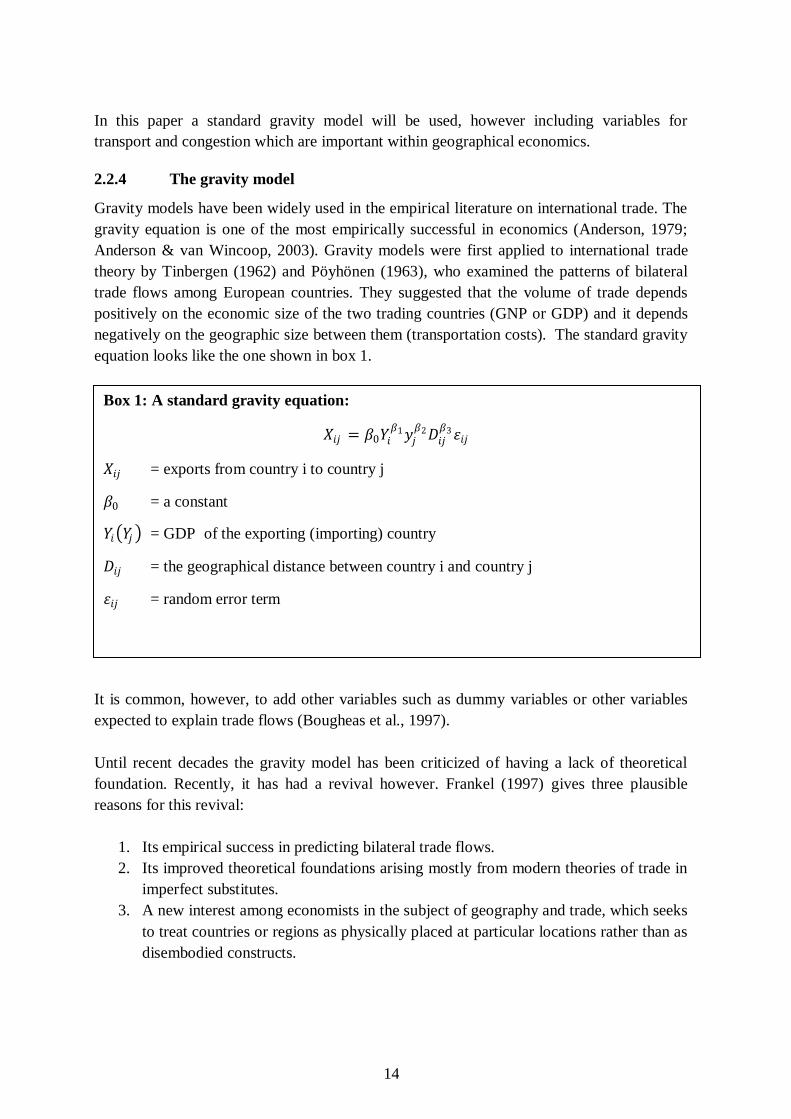
equation looks like the one shown in box 1.

It is common, however, to add other variables such as dummy variables or other variables

expected to explain trade flows (Bougheas et al., 1997).

Until recent decades the gravity model has been criticized of having a lack of theoretical

foundation. Recently, it has had a revival however. Frankel (1997) gives three plausible

reasons for this revival:

1. Its empirical success in predicting bilateral trade flows.

2. Its improved theoretical foundations arising mostly from modern theories of trade in

imperfect substitutes.

3. A new interest among economists in the subject of geography and trade, which seeks

to treat countries or regions as physically placed at particular locations rather than as

disembodied constructs.

𝑋𝑖𝑗 = 𝛽0𝑌𝑖𝛽1𝑦𝑗

𝛽2𝐷𝑖𝑗𝛽3𝜀𝑖𝑗

Box 1: A standard gravity equation:

𝑋𝑖𝑗 = exports from country i to country j

𝛽0 = a constant

𝑌𝑖 𝑌𝑗 = GDP of the exporting (importing) country

𝐷𝑖𝑗 = the geographical distance between country i and country j 𝜀𝑖𝑗 = random error term

15

The theoretical underpinning of the gravity equation started with Anderson (1979). He

derived a gravity equation from the properties of expenditure systems. Bergstrand (1985)

introduced a general equilibrium model of world trade. By making some simplifying

assumptions, such as perfect substitutability of goods across countries, he derives a gravity

equation. More recently, Deardorff (1995) derives a gravity equation from two extreme

cases of the H-O model: one with frictionless trade7 and another one with countries that each

produce different goods. Lately, the gravity model has been used by many to estimate the

effects of infrastructure on trade. Bougheas et al., (1997) develop a model where transport

costs are not only a function of distance but also of public infrastructure. They include a

variable for public infrastructure in their model. However, since that variable also includes

non-transport related infrastructure, they use a second model to measure the direct effect of

transport infrastructure. The variable they use for that is the length of motorway network.

Limão & Venables (2001) also use a gravity equation to find the role of infrastructure in

explaining trade volumes. They include dummies for a common border and for being an

island in the model. Other variables they added were first of all an inverse of the index of

road, paved road, and railway densities and telephone lines per capita. In this case, a higher

value indicates worse infrastructure. A second other variable they added an average value of

infrastructure for the transit countries if a country is landlocked, if it is a coastal country the

value is zero. Finally, Acosta Rojas et al. (2005) similarly test the effects of infrastructure on

trade volumes. They modify the distance variable from the standard gravity equation by an

infrastructure index.

7 In this case, the absence of all barriers to trade in homogenous products causes producers and consumers to

be indifferent among trading partners, including their own country, as long as they buy or sell the desired

good (Deardorff, 1995)

16

3 Methodology

This section will discuss properties of the model that will be used in this study. First of all,

the advantages of panel data are discussed. Accordingly, the fixed effects- and random

effects models, which are the most common models when using panel data, are pointed out.

In the second subsection, the variables of the model will be explained.

3.1 Model estimation

3.1.1 Panel data

As stated in the introduction, this model will use panel data for the 12 South American

countries in the time period 1993 – 1999. The reason to use panel data in this research is that

the sample of countries is very small. Thereby, the time period is not that large either.

Combining cross-sectional data with time series will give a much larger dataset and

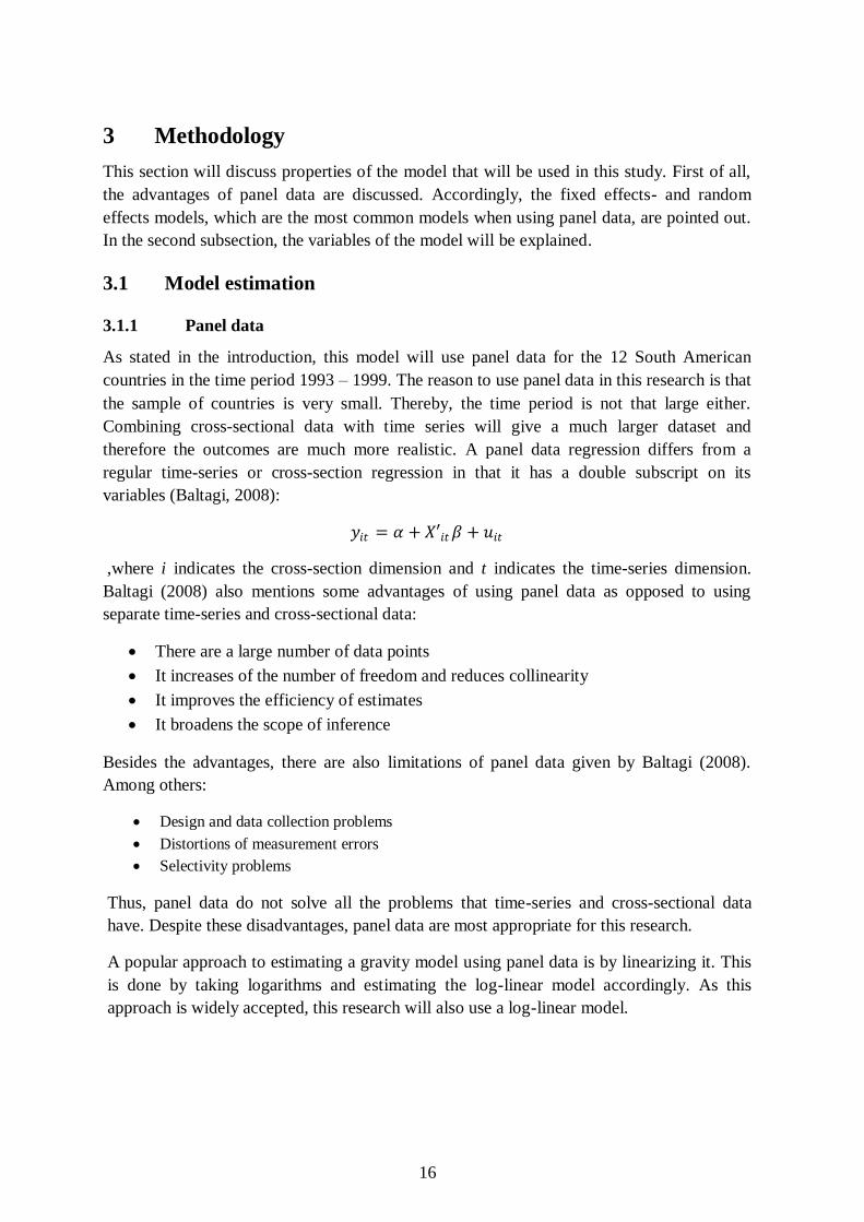
therefore the outcomes are much more realistic. A panel data regression differs from a

regular time-series or cross-section regression in that it has a double subscript on its

variables (Baltagi, 2008):

𝑦𝑖𝑡 = 𝛼 + 𝑋′𝑖𝑡𝛽 + 𝑢𝑖𝑡

,where i indicates the cross-section dimension and t indicates the time-series dimension.

Baltagi (2008) also mentions some advantages of using panel data as opposed to using

separate time-series and cross-sectional data:

There are a large number of data points

It increases of the number of freedom and reduces collinearity

It improves the efficiency of estimates

It broadens the scope of inference

Besides the advantages, there are also limitations of panel data given by Baltagi (2008).

Among others:

Design and data collection problems

Distortions of measurement errors

Selectivity problems

Thus, panel data do not solve all the problems that time-series and cross-sectional data

have. Despite these disadvantages, panel data are most appropriate for this research.

A popular approach to estimating a gravity model using panel data is by linearizing it. This

is done by taking logarithms and estimating the log-linear model accordingly. As this

approach is widely accepted, this research will also use a log-linear model.

17

3.1.2 Fixed effects and random effects

There are several types of panel analytic model. The most common ones, the fixed effects-

and random effects model, will be discussed in more detail. A fixed effects model can be

explained by the following simple linear model:

𝑌𝑖𝑗 = 𝛽0 + 𝛽1𝑥𝑖𝑗 + 𝛼𝑖 + 𝜀𝑖𝑗

In the above model 𝛼𝑖 represents individual specific effects. When the intercepts are

different across countries but do not differ over time, then it is a fixed effects model. Thus, a

fixed effect model explores the relationship between predictor and outcome variable within

an entity. The fixed effects model controls for all the time-invariant differences between the

entities, so the estimated coefficients cannot be biased because of omitted time-invariant

characteristics. (Torres-Reyna, 2007)

A random effects model can be explained by the following simple linear model:

𝑌𝑖𝑗 = 𝛽𝑥𝑖𝑗 + 𝛼𝑖 + 𝑢𝑖𝑗 + 𝜀𝑖𝑗

, where 𝑢𝑖𝑗 is the between-entity error term. In the random effects model the variation

between the entities is assumed to be random and uncorrelated with the explanatory

variables in the model. Thus, with a random effects model the effects of a stable covariate

variable, e.g. race, can be estimated.

In the literature, the fixed effects model is mostly used. However, this does not mean that the

model in this research would be estimated best by using fixed effects as well. A Hausman

test can be used to find whether fixed- or random effects are most appropriate. This is

further discussed in section 4.

3.2 A gravity model with transport infrastructure

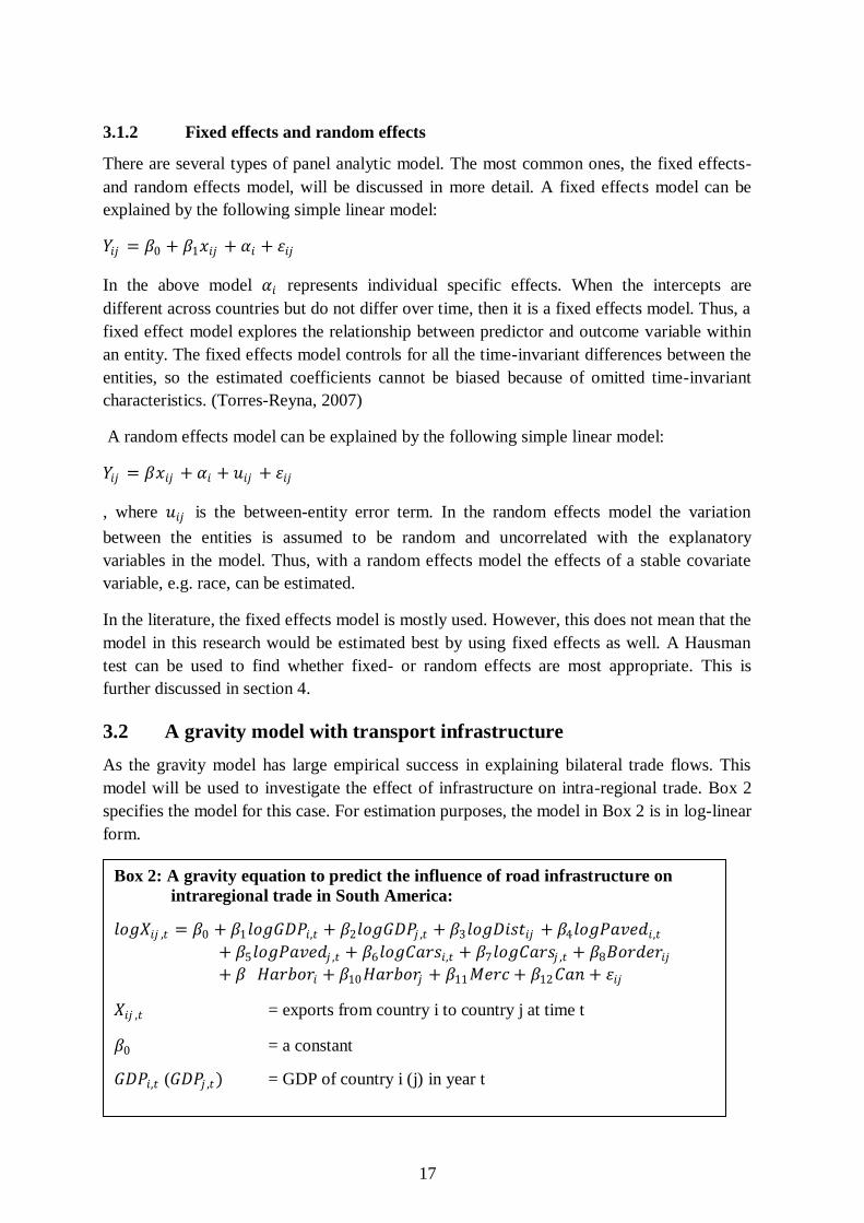
As the gravity model has large empirical success in explaining bilateral trade flows. This

model will be used to investigate the effect of infrastructure on intra-regional trade. Box 2

specifies the model for this case. For estimation purposes, the model in Box 2 is in log-linear

form.

𝑙𝑜𝑔𝑋𝑖𝑗 ,𝑡 = 𝛽0 + 𝛽1𝑙𝑜𝑔𝐺𝐷𝑃𝑖,𝑡 + 𝛽2𝑙𝑜𝑔𝐺𝐷𝑃𝑗 ,𝑡 + 𝛽3𝑙𝑜𝑔𝐷𝑖𝑠𝑡𝑖𝑗 + 𝛽4𝑙𝑜𝑔𝑃𝑎𝑣𝑒𝑑𝑖,𝑡

+ 𝛽5𝑙𝑜𝑔𝑃𝑎𝑣𝑒𝑑𝑗 ,𝑡 + 𝛽6𝑙𝑜𝑔𝐶𝑎𝑟𝑠𝑖,𝑡 + 𝛽7𝑙𝑜𝑔𝐶𝑎𝑟𝑠𝑗 ,𝑡 + 𝛽8𝐵𝑜𝑟𝑑𝑒𝑟𝑖𝑗+ 𝛽 𝐻𝑎𝑟𝑏𝑜𝑟𝑖 + 𝛽10𝐻𝑎𝑟𝑏𝑜𝑟𝑗 + 𝛽11𝑀𝑒𝑟𝑐+ 𝛽12𝐶𝑎𝑛 + 𝜀𝑖𝑗

Box 2: A gravity equation to predict the influence of road infrastructure on

intraregional trade in South America:

𝑋𝑖𝑗 ,𝑡 = exports from country i to country j at time t

𝛽0 = a constant

𝐺𝐷𝑃𝑖,𝑡 (𝐺𝐷𝑃𝑗 ,𝑡) = GDP of country i (j) in year t

18

3.2.1 The dependent variable

Bilateral exports were chosen to be the dependent variable in this gravity equation. It should

not make a large difference whether imports or exports are used since one country‟s imports

are the other country‟s exports. However, there are always some discrepancies between

imports and export reported by the two trading countries. This can be due to timing or

including/excluding particular commodities (United Nations, 2010). Furthermore, countries

do also not always report in the latest classification. Thus, when evaluating the data, these

discrepancies should be taken into account.

3.2.2 Explanatory variables

GDP

The GDP variable is a basic variable in the gravity equation. It is expected that when GDP

increases, the trade volume will go up as well. In other words, a positive relationship is

expected.

Geographical distance

Geographical distance between countries will be measured by taking the distance between

the capital cities of the countries in kilometers. In South America most of the economic

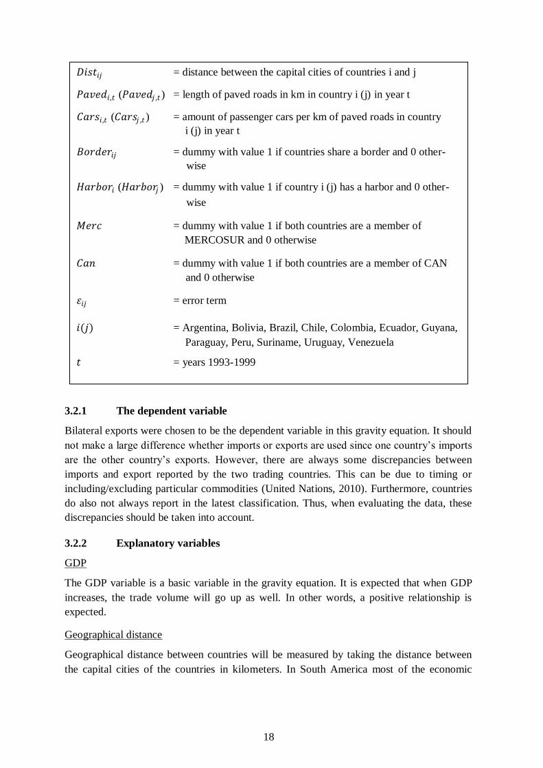
𝐷𝑖𝑠𝑡𝑖𝑗 = distance between the capital cities of countries i and j

𝑃𝑎𝑣𝑒𝑑𝑖,𝑡 (𝑃𝑎𝑣𝑒𝑑𝑗 ,𝑡 ) = length of paved roads in km in country i (j) in year t

𝐶𝑎𝑟𝑠𝑖,𝑡 (𝐶𝑎𝑟𝑠𝑗 ,𝑡 ) = amount of passenger cars per km of paved roads in country

i (j) in year t

𝐵𝑜𝑟𝑑𝑒𝑟𝑖𝑗 = dummy with value 1 if countries share a border and 0 other-

wise

𝐻𝑎𝑟𝑏𝑜𝑟𝑖 (𝐻𝑎𝑟𝑏𝑜𝑟𝑗 ) = dummy with value 1 if country i (j) has a harbor and 0 other-

wise

𝑀𝑒𝑟𝑐 = dummy with value 1 if both countries are a member of

MERCOSUR and 0 otherwise

𝐶𝑎𝑛 = dummy with value 1 if both countries are a member of CAN

and 0 otherwise

𝜀𝑖𝑗 = error term

𝑖(𝑗) = Argentina, Bolivia, Brazil, Chile, Colombia, Ecuador, Guyana,

Paraguay, Peru, Suriname, Uruguay, Venezuela

𝑡 = years 1993-1999

19

activity happens in these cities, thus most of the trade is between those cities as well.8

Distance is expected to, as is generally stated in the literature, negatively affect trade.

Paved roads and congestion

Much of the literature on the effect of infrastructure on trade has been concentrated on

transportation costs. However, as this research is focusing on road transport specifically,

some other variables will be considered to explain trade. First of all, in the line of Bougheas

et al. (1997) who take the length of the motorway network as a variable, this model includes

the total length of paved roads in the trading countries as a measure of the quantity of

infrastructure. It is expected that the higher the length of paved roads, the higher will be

trade. Bougheas at al. (1997) found that scaling this road infrastructure measure by distance

does not give a significant difference in the results, therefore this is not done in this study.

Secondly, literature on geographical economics talks very much about congestion and

congestion costs. In several studies it has been stated that it is not only the quantity but also

the quality of the infrastructure that affects trade. In this study it is assumed that congestion

is a factor that lowers the quality and therefore it will negatively influence trade.

Congestion will be measured by the amount of passenger cars per kilometer of road and it is

supposed to have a negative influence on trade. Another measure for the quality of

infrastructure, besides congestion, could be safety. Safety could be measured by the number

of people killed in road traffic accidents. If this rate is high, it means there is a high risk

driving on a road in that particular country, or, in other words, the quality is low. Hence, the

number of people killed in road traffic accident is expected to have a negative effect on

trade. Because of the lack of data on road accidents in South America, this study will leave

road accidents out of the model. Quality of the roads will therefore only be measured by

congestion.

3.2.3 Dummy variables

Dummy variables are added to the model to control for categorical effects. First of all, a

dummy for common borders is included. A common border eases trade between two

countries, and trade will therefore usually be higher. A value of one is therefore assigned if

the two trading countries have a common border and a zero otherwise. A second dummy is

included for harbors. This study concentrates on road infrastructure as most of the

intraregional trade in South America goes via the road. A good second place is, however, for

transport by ship. The use of other ways of transportation in intraregional is almost nil.

Thus, a dummy for harbors is included to control for transport per ship. The value of one is

assigned if a country has a harbor, the coastal countries, and a zero is assigned if the country

does not have a harbor, the land-locked countries. Finally, dummies are assigned to control

8 In Brazil the point of measurement is São Paolo as this is where most of the economic activities of Brazil take

place.

20

for the regional trade agreements of MERCOSUR9 and the CAN

10. If both countries are a

member of the agreement the value of 1 is assigned if only one of them or none of them are

a member the value of 0 is assigned.

3.2.4 Data collection

Data is collected from several resources. First of all, data for exports is retrieved from the

statistical database of the United Nations, UN Comtrade. GDP data for all countries is taken

from the Latin American and Caribbean Macro Watch Data Tool of the Inter American

Development Bank. The geographical distance between countries is measured using Google

Earth. The distance taken is the distance as the crow flies, thus not the distance it would be

via the road. All data with respect to the total length of roads, the total length of paved roads,

and the amount of passenger cars per kilometer of road is retrieved from the World Road

Statistics database of the International Road Federation.

9 The MERCOSUR full member countries during the period 1993-1999 are: Argentina, Brazil, Paraguay, and

Uruguay.

10 The CAN full member countries during the period 1993-1999 are: Bolivia, Colombia, Ecuador, Peru, and

Venezuela.

21

4 Statistical methods

Before estimating the model, some corrections in the sample data are made. As there is

much missing data for Guyana and Suriname, these countries will be excluded from the

sample. As there is some missing data in the sample, an unbalanced panel will be used in the

analysis. In the following sections it will be further described how the model is statistically

estimated.

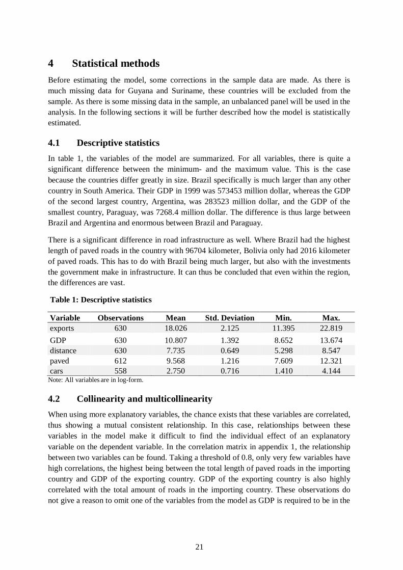
4.1 Descriptive statistics

In table 1, the variables of the model are summarized. For all variables, there is quite a

significant difference between the minimum- and the maximum value. This is the case

because the countries differ greatly in size. Brazil specifically is much larger than any other

country in South America. Their GDP in 1999 was 573453 million dollar, whereas the GDP

of the second largest country, Argentina, was 283523 million dollar, and the GDP of the

smallest country, Paraguay, was 7268.4 million dollar. The difference is thus large between

Brazil and Argentina and enormous between Brazil and Paraguay.

There is a significant difference in road infrastructure as well. Where Brazil had the highest

length of paved roads in the country with 96704 kilometer, Bolivia only had 2016 kilometer

of paved roads. This has to do with Brazil being much larger, but also with the investments

the government make in infrastructure. It can thus be concluded that even within the region,

the differences are vast.

Table 1: Descriptive statistics

Variable Observations Mean Std. Deviation Min. Max.

exports 630 18.026 2.125 11.395 22.819

GDP 630 10.807 1.392 8.652 13.674

distance 630 7.735 0.649 5.298 8.547

paved 612 9.568 1.216 7.609 12.321

cars 558 2.750 0.716 1.410 4.144 Note: All variables are in log-form.

4.2 Collinearity and multicollinearity

When using more explanatory variables, the chance exists that these variables are correlated,

thus showing a mutual consistent relationship. In this case, relationships between these

variables in the model make it difficult to find the individual effect of an explanatory

variable on the dependent variable. In the correlation matrix in appendix 1, the relationship

between two variables can be found. Taking a threshold of 0.8, only very few variables have

high correlations, the highest being between the total length of paved roads in the importing

country and GDP of the exporting country. GDP of the exporting country is also highly

correlated with the total amount of roads in the importing country. These observations do

not give a reason to omit one of the variables from the model as GDP is required to be in the

22

gravity equation and the road and paved road variables have a different purpose in

explaining trade flows than GDP has. Furthermore, the correlation table shows high

correlation between total length of roads and total length of paved roads. As they have the

same purpose in explaining trade, they are both a proxy for infrastructure; therefore, one of

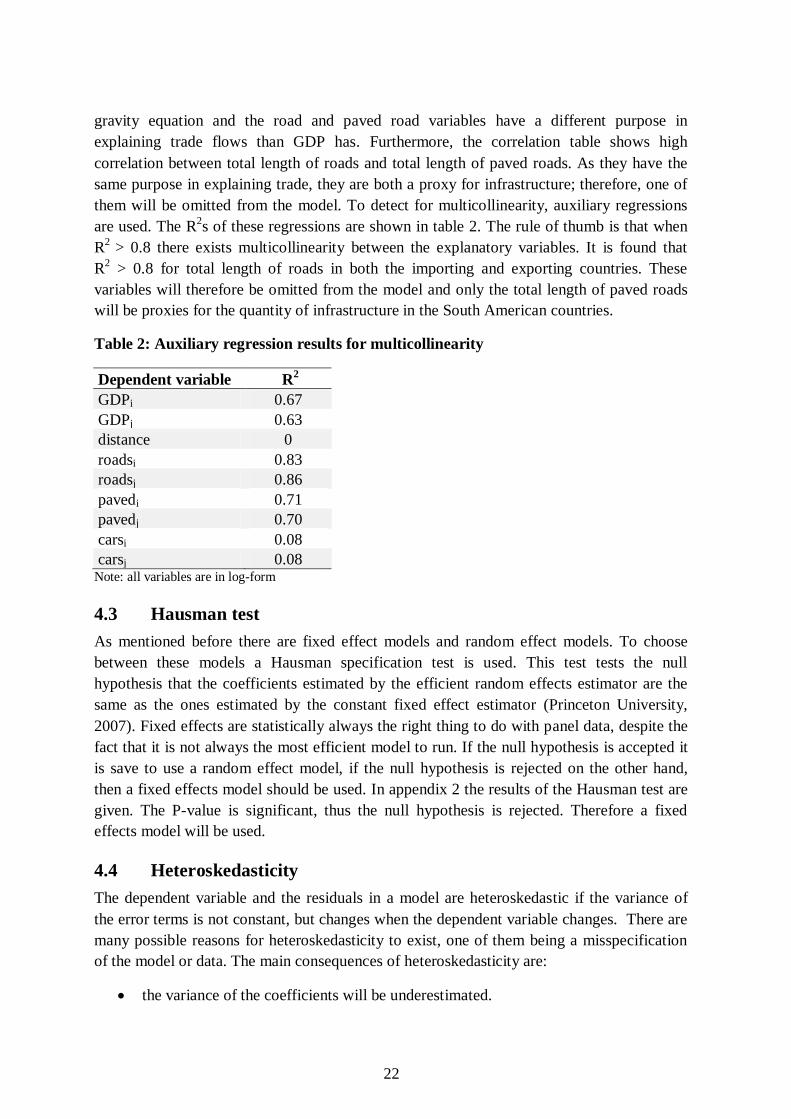
them will be omitted from the model. To detect for multicollinearity, auxiliary regressions

are used. The R2s of these regressions are shown in table 2. The rule of thumb is that when

R2

> 0.8 there exists multicollinearity between the explanatory variables. It is found that

R2 > 0.8 for total length of roads in both the importing and exporting countries. These

variables will therefore be omitted from the model and only the total length of paved roads

will be proxies for the quantity of infrastructure in the South American countries.

Table 2: Auxiliary regression results for multicollinearity

Dependent variable R2

GDPi 0.67

GDPj 0.63

distance 0

roadsi 0.83

roadsj 0.86

pavedi 0.71

pavedj 0.70

carsi 0.08

carsj 0.08 Note: all variables are in log-form

4.3 Hausman test

As mentioned before there are fixed effect models and random effect models. To choose

between these models a Hausman specification test is used. This test tests the null

hypothesis that the coefficients estimated by the efficient random effects estimator are the

same as the ones estimated by the constant fixed effect estimator (Princeton University,

2007). Fixed effects are statistically always the right thing to do with panel data, despite the

fact that it is not always the most efficient model to run. If the null hypothesis is accepted it

is save to use a random effect model, if the null hypothesis is rejected on the other hand,

then a fixed effects model should be used. In appendix 2 the results of the Hausman test are

given. The P-value is significant, thus the null hypothesis is rejected. Therefore a fixed

effects model will be used.

4.4 Heteroskedasticity

The dependent variable and the residuals in a model are heteroskedastic if the variance of

the error terms is not constant, but changes when the dependent variable changes. There are

many possible reasons for heteroskedasticity to exist, one of them being a misspecification

of the model or data. The main consequences of heteroskedasticity are:

the variance of the coefficients will be underestimated.

23

standard errors in the model are wrong and as a result the hypothesis tests can be

incorrect.

Heteroskedasticity in a fixed effects model can be easily detected by a modified Wald test

for groupwise heteroskedasticity. In appendix 3 the results are shown. In this test the null

hypothesis is homoskedasticity. It is found that Prob > chi2 = 0.0000, thus the null

hypothesis can be rejected, which suggests that heteroskedasticity is present. Therefore, in

the model will be controlled for heteroskedasticity.

4.5 Autocorrelation

Autocorrelation is often detected in time-series- and pooled time-series data. Autocorrelation

represents the level of similarity between a given time series and a lagged version of itself

over successive time intervals. As a result information obtained from the independent

variables can be due to the data of previous years. The consequences of autocorrelation are

similar to those of heteroskedasticity. To test this model on autocorrelation, a Wooldridge

test for autocorrelation in panel data is done. The results of this test are shown in appendix 4.

The null hypothesis is no first-order autocorrelation. As Prob > F = 0.0013, the null

hypothesis can be rejected. Thus, autocorrelation is present in the model and should be

corrected for.

24

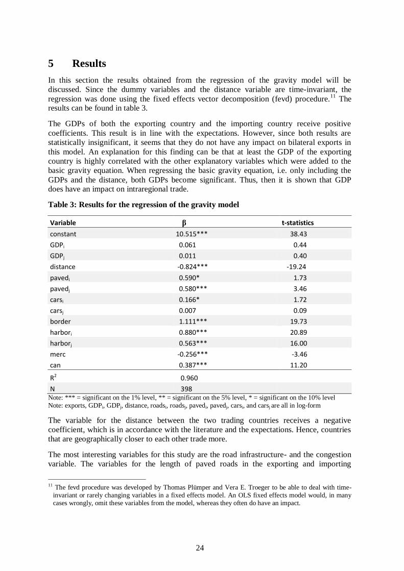
5 Results

In this section the results obtained from the regression of the gravity model will be

discussed. Since the dummy variables and the distance variable are time-invariant, the

regression was done using the fixed effects vector decomposition (fevd) procedure.11

The results can be found in table 3.

The GDPs of both the exporting country and the importing country receive positive

coefficients. This result is in line with the expectations. However, since both results are

statistically insignificant, it seems that they do not have any impact on bilateral exports in

this model. An explanation for this finding can be that at least the GDP of the exporting

country is highly correlated with the other explanatory variables which were added to the

basic gravity equation. When regressing the basic gravity equation, i.e. only including the

GDPs and the distance, both GDPs become significant. Thus, then it is shown that GDP does have an impact on intraregional trade.

Table 3: Results for the regression of the gravity model

Variable β t-statistics

constant 10.515*** 38.43

GDPi 0.061 0.44

GDPj 0.011 0.40

distance -0.824*** -19.24

pavedi 0.590* 1.73

pavedj 0.580*** 3.46

carsi 0.166* 1.72

carsj 0.007 0.09

border 1.111*** 19.73

harbori 0.880*** 20.89

harborj 0.563*** 16.00

merc -0.256*** -3.46

can 0.387*** 11.20

R2 0.960

N 398 Note: *** = significant on the 1% level, ** = significant on the 5% level, * = significant on the 10% level

Note: exports, GDPi, GDPj, distance, roadsi, roadsj, pavedi, pavedj, carsi, and carsj are all in log-form

The variable for the distance between the two trading countries receives a negative

coefficient, which is in accordance with the literature and the expectations. Hence, countries

that are geographically closer to each other trade more.

The most interesting variables for this study are the road infrastructure- and the congestion

variable. The variables for the length of paved roads in the exporting and importing

11 The fevd procedure was developed by Thomas Plümper and Vera E. Troeger to be able to deal with time-

invariant or rarely changing variables in a fixed effects model. An OLS fixed effects model would, in many

cases wrongly, omit these variables from the model, whereas they often do have an impact.

25

countries are both given positive coefficients and are also statistically significant. Thus, the

higher the length of paved roads in the South American countries, the higher the bilateral

exports within the region will be. The first hypothesis is therefore accepted. Congestion was

tested by the amount of cars per kilometer of road in the exporting and importing country.

The variables were both given a positive sign, which is against the expectations. For the

exporting country this effect is significant. This is not the case for the importing country

though. Therefore, the amount of cars per kilometer of road in the importing country does

not have an impact on bilateral exports. It was presumed that congestion would have a

negative impact on the amount of bilateral exports. The second hypothesis is therefore

rejected. A reason for this variable not having the right sign can be that economic activity in

South America mainly takes place in a few large cities where congestion is high. As the

amount of cars is measured per kilometer of road through the whole country, congestion

appears to be much lower than it is in reality. A better measure could therefore be the

amount of cars per city.

The border and harbor dummy variables all have positive coefficients. For the border

dummy this is in line with previous literature, where it is claimed that countries bordering

each other trade more. In this model this variable seems to be the most important one in

choosing the export partner as the coefficient is the highest. This confirms what Acosta

Rojas et al. (2005) found in their study about trade in the Andean community. Especially

because most trade happens via the road, a logical result is that countries bordering each

other trade more. Since much trade happens over sea as well, it was expected that having a

harbor has a positive influence on bilateral exports. Being a member of CAN significantly

influences intraregional trade positively, which is in line with the expectations. On the other

hand, being a member of MERCOSUR seems to have a significant negative influence on

bilateral exports, which is against expectations. Free trade zones are set up to improve trade

between the member countries. Evidence for this is found by many previous empirical

studies. However, in this model, for the MERCOSUR agreement this is not the case. A

possible explanation for this finding is that free trade zones in South America are still

imperfect and that they are therefore not per se positively influencing trade between the

member countries. A similar finding was done by Carillo & Li (2004). They also find a

significant positive influence of the CAN agreement and no significant positive influence of the MERCOSUR agreement on trade.

The R2 in this model is 0.960, which is very high. This indicates that this model does very

well in explaining bilateral exports within South America. The high amount of significant

coefficients further confirms this result. The constant is significant at the 1% level, but this

only tells us that the constant is significantly different from zero.

26

6 Granger causality tests

As stated in the introduction, the second research question deals with the relation between

trade and economic growth. It is hypothesized there that trade causes growth.

In section 2 it is mentioned, however, that literature found evidence of the causality going in

both directions. Therefore, to determine the direction of causality between trade and GDP

growth in South America, Granger causality tests are done for all ten countries used in the

gravity model. Thus, Guyana and Suriname are also left out of the analysis here. Data for

exports and imports for the years 1962-2008 are retrieved from UN Comtrade, and data for

GDP growth per capita is taken from the World databank.

Granger causality relies on the idea that the chance of something that occurs in a later period

of time is caused by something that happens before is larger than vice versa. In other words,

it is based on a chronological idea of causality. Nevertheless, there is always a chance that

actors anticipate to expected happenings which turns around the time idea.

It should be noted that in this paper Granger causality is not necessarily true causality. The

Granger causality tests are rather an attempt to state a requirement for a causal relation.

6.1 Statistical methods

Granger causality tests need data to be stationary, in other words there should not be an

obvious time trend in the data. Since there is a trend in the data and the variance is

proportional to the mean, the trade data were first transformed to their logarithmic form. In

the graph in appendix 6 it is seems that the intraregional trade data of Argentina is non-

stationary. This is true for all data with respect to intraregional-, extraregional-, and total

trade of all the ten tested countries.12

Following this result, the series were all checked

separately for stationarity using an Augmented Dickey-Fuller (ADF) test. This test examines

whether a series has a unit root. If it does, it means the series is non-stationary. By

differencing the data, the series can be made stationary. In general it is sufficient to take the

first difference, only occasionally the second difference is needed to make data stationary. If

taking the first difference makes data stationary, it is said to be integrated of order one.

6.2 Results of the Granger causality tests

The first line of appendix 5 shows that the intraregional trade data of Argentina has a unit

root; the ADF test statistic is higher than the critical values. Thereby, the Durbin-Watson

statistic is not so high which means that there is evidence of positive serial correlation. The

extraregional- and total trade series of Argentina as well as intraregional-, extraregional, and

total trade data of the nine other tested countries also included a unit root and therefore all

these trade series are non-stationary. On the other hand, none of the GDP growth series had

a unit root. Thus, the GDP growth series are all stationary. As all trade data have a unit root,

12 Extraregional trade is defined by trade between the South American countries and the rest of the world.

27

the next step is doing the ADF test taking the first difference. Appendix 5 shows that now

the ADF test statistic is lower than the critical values and it further shows a Durbin-Watson

statistic which is higher than two. Hence, there is no autocorrelation. The same results were

found for the extraregional- and total trade series of Argentina as well as intraregional-,

extraregional, and total trade data series of the nine other tested countries. The graph in

appendix 7 shows the intraregional data of Argentina after having it differenced. In this

graph there is clearly no time trend to be spot, thus the data is stationary.

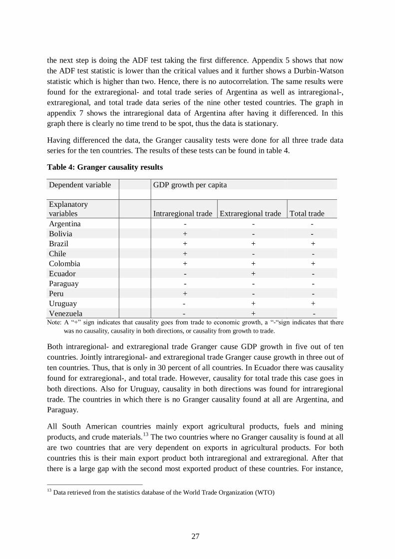
Having differenced the data, the Granger causality tests were done for all three trade data

series for the ten countries. The results of these tests can be found in table 4.

Table 4: Granger causality results

Dependent variable GDP growth per capita

Explanatory

variables Intraregional trade Extraregional trade Total trade

Argentina - - -

Bolivia + - -

Brazil + + +

Chile + - -

Colombia + + +

Ecuador - + -

Paraguay - - -

Peru + - -

Uruguay - + +

Venezuela - + - Note: A “+” sign indicates that causality goes from trade to economic growth, a “-“sign indicates that there

was no causality, causality in both directions, or causality from growth to trade.

Both intraregional- and extraregional trade Granger cause GDP growth in five out of ten

countries. Jointly intraregional- and extraregional trade Granger cause growth in three out of

ten countries. Thus, that is only in 30 percent of all countries. In Ecuador there was causality

found for extraregional-, and total trade. However, causality for total trade this case goes in

both directions. Also for Uruguay, causality in both directions was found for intraregional

trade. The countries in which there is no Granger causality found at all are Argentina, and

Paraguay.

All South American countries mainly export agricultural products, fuels and mining

products, and crude materials.13

The two countries where no Granger causality is found at all

are two countries that are very dependent on exports in agricultural products. For both

countries this is their main export product both intraregional and extraregional. After that

there is a large gap with the second most exported product of these countries. For instance,

13 Data retrieved from the statistics database of the World Trade Organization (WTO)

28

total exports of agricultural products for Argentina in 2008 had a value of 37502 million US

dollars. In the same year, the second largest export product for the country was machinery

and transport equipment with a value of 9746 million US dollars. Comparing this to Brazil,

whose main export product is agricultural products (with a value of 61400 million US

dollars) as well but exports many fuels and mining products too (with a value of 44020

million US dollars), it can be seen that Argentina is much more dependent on agricultural

products only.14

The same is true for Paraguay, who basically only exports agricultural

products. Besides Brazil and Uruguay, whose main export product is agricultural products as

well, the other South American countries mainly export fuels and mining products. Hence, it

can be concluded that there is evidence found for trade causing GDP growth in the countries

that are mainly depending on the exports of fuels and mining products in their trade.

Since this paper is especially interested in the effects of intraregional trade it is interesting to

have a more detailed look at that. As mentioned in section 6.2, Granger causality is found

for five out of ten countries for intraregional trade. These countries have fuels and mining

products as a main export product, but so do Ecuador and Venezuela. The difference

between these two countries and the countries for which causality is found is that also within

the region, Ecuador and Venezuela mainly export fuels and mining products, whereas

Brazil‟s , Chile‟s, Colombia‟s, and Peru‟s exports are much more mixed within the region.

Thereby, the exports of Ecuador and Venezuela go for more than 80 percent to only two

other countries in the region. For Brazil, Chile, Colombia, and Peru, the exports are going to

many different countries in the region. The only country that does not follow this analysis is

Bolivia. More than 75 percent of the country‟s exports go to Brazil, and these are also

basically only fuel and mining products. A reason for the deviation from Bolivia in the

pattern could be that the country is much poorer than the other countries in the region

However, no evidence is found to confirm this.

14 The values of total exports per commodity were retrieved from the statistics database of the World Trade

Organization (WTO)

29

7 Conclusion

The purpose of this paper was to analyze the effect of infrastructure determinants on

bilateral exports within South America. To accomplish this purpose, using a gravity model,

a regression was run on bilateral trade from ten South American countries over the years

1993-1999. One of the IIRSA‟s ultimate goals is to promote sustainable growth. Therefore,

in addition the relationship between trade and economic growth was analyzed using Granger

causality tests for the same ten countries separately. The following hypotheses were tested:

H1: The quantity of road infrastructure positively influences intraregional trade in South

America.

H2: The quality of road infrastructure positively influences intraregional trade in South

America.

H3: Intraregional trade causes economic growth

The regression results of the gravity equation showed that the amount of paved roads does

have a positive impact on intraregional trade in South America. This finding supports that a

larger quantity of transport infrastructure increases trade. The study does however not find

evidence for a negative impact of congestion on intraregional trade in South America. In

other words, no evidence is found for a better quality of infrastructure improving trade in the

region. A reason for this variable not having the right sign can be that economic activity in

South America mainly takes place in a few large cities where congestion is high. As the

amount of cars is measured per kilometer of road through the whole country, congestion

appears to be much lower than it is in reality. A better measure could therefore be the

amount of cars per city.

The results of the Granger causality tests indicate that for 50 percent of the South American

countries intraregional trade causes economic growth. Furthermore, in 30 percent of the

countries, total trade was found to cause economic growth. Thus, it should be noted that

trade does not always cause growth in South America. The differences in the results for the

various countries could be explained by the type of products that are mainly exported by the

countries. No empirical evidence is found for that in this study though.

The IIRSA chose to concentrate on improving transport infrastructure to improve

intraregional trade instead of concentrating on developing the free trade zones to ones that

are more perfect. It seems that this is a good choice, as a greater quantity infrastructure does

indeed have a positive effect on trade within the region. Therefore, it is likely that when the

IIRSA has finished all its projects, intraregional trade in South America will be at a fairly

higher level than it is nowadays. Furthermore, transport infrastructure is an easy manageable

variable for the governments of the countries. In addition to that, for free trade areas to work

better, it is necessary that the countries are interlinked in a good way first. Finally,

developing infrastructure is not only a tool to increase intraregional trade in South America.

30

It is also a way to development overall, including more integration and higher economic

growth.

Although road transport is the main mode of transportation used for intraregional trade in

South America, a suggestion for future research would be to not only look at road

infrastructure but also at the infrastructure of other transport modes, including water-,

railway, and air transport, and their influence on intraregional trade. In line with this, it

could be investigated whether other modes of transport could be better explored and play a

larger role in intraregional trade. Another suggestion is to also look better at the influence of

trade on economic growth. This study looked at the causal relation between, but it lacks

numbers on the amount of influence intraregional trade would have. A growth model

including some indicator of intraregional trade could then be used to find the amount of

influence of intraregional trade on economic growth. From that, one could then draw

conclusions about whether South America should indeed focus on intraregional trade or that

it is an overrated factor in the development of the region. Finally, to find out whether the

projects of the IIRSA did help increasing intraregional trade, a similar research to the one

carried out in this paper could be conducted after the projects have been finished.

31

References

Acosta Rojas, G. E., Calfat, G., & Flôris Jr, R. G. (2005). Trade and infrastructure:

evidences from the Andean community. Ensaios Econômicos, 580.

Anderson, J. E. (1979). A theoretical foundation for the gravity equation. The American

Economic Review, 69(1), 106-116.

Anderson, J. E., & van Wincoop, E. (2003). Gravity with gravitas: a solution to the border

puzzle. The American Economic Review, 93(1), 170-192.

Anderson, J. E., & van Wincoop, E. (2004). Trade costs. Journal of Economic Literature,

42, 691-751.

Aschauer, D. A. (1989). Is public expenditure productive? Journal of Monetary Economics,

23, 177-200.

Baltagi, B. H. (2008). Econometric analysis of panel data (fourth ed.). Chippenham: John

Wiley & Sons Ltd.

Bassasini, A., & Scarpetta, S. (2001). The driving forces of economic growth: panel data

evidence for the OECD countries. OECD Economic Studies, 33(2001/2).

Bergstrand, J. H. (1985). The gravity equation in international trade: some microeconomic

foundations and empirical evidence. The Review of Economics and Statistics, 67(3),

474-481.

Bougheas, S., Demetriades, P. O., & Mamuneas, T. P. (2000). Infrastructure, specialization,

and economic growth. Canadian Journal of Economics, 33(2), 506-522.

Bougheas, S., Demetriades, P. O., & Morgenroth, E. L. W. (1997). Infrastructure, transport

costs, and trade. Journal of International Economics, 47, 169-189.

Brakman, S., Garretsen, H., & van Marrewijk, C. (2009). The new introduction to

geographical economics (second ed.). New York: Cambridge University Press.

Briceño-Garmendia, C., Estache, A., & Shafik, N. (2004). Infrastructure services in

developing countries: access, quality, costs, and policy reform o. Document

Number)

Calderon, C., & Servén, L. (2002). The output cost of Latin America's infrastructure gap o.

Document Number)

Calderon, C., & Servén, L. (2004). The effects of infrastructure development on growth and

income distribution o. Document Number)

Carillo, C., & Li, C. A. (2004). Trade blocks and the gravity model: evidence from Latin

American countries. Journal of Economic Integration, 19(4), 667-689.

Cuadros, A., Orts, V., & Alguacil, M. T. (2004). Openness and growth: Re-examining

foreign directs investment, trade, and output linkages in Latin America. CREDIT

Research Paper no. 01/04.

Deardorff, A. V. (1995). Determinants of bilateral trade: does gravity work in a

neoclassical world? Paper presented at the Regionalization of the World Economy.

Dixit, A., & Stiglitz, J. E. (1977). Monopolistic competition and optimum product diversity.

The American Economic Review, 67(3), 297-308.

Edwards, S. (1992). Trade orientation, distortions and growth in developing countries.

Journal of Development Economics, 39, 31-57.

Fay, M., & Morrison, M. (2007). Infrastructure in Latin America and the Caribbean: recent

developments and key challenges. Washington: The World Bank.

Frankel, J. A. (1997). Regional trading blocs in the world economic system. Washington:

Institute for International Economics.

32

Frankel, J. A., & Romer, D. (1999). Does trade cause growth? The American Economic

Review, 89(3), 379-399.

Gramlich, E. M. (1994). Infrastructure investment: a review essay. Journal of Economic

Literature, 32, 1176-1196.

Grossmann, G. M., & Helpman, E. (1990a). Trade, innovation, and growth. American

Economic Review, 80(2), 86-91.

Grossmann, G. M., & Helpman, E. (1990b). Trade, knowledge spillovers, and growth.

NBER working paper no. 3485.

Harrison, A. (1996). Openness and growth: A time-series, cross-country analysis for

developing countries. Journal of Development Economics, 48, 419-447.

Head, K., & Mayer, T. (2004). The empirics of agglomeration and trade. In J. V. Henderson

& J.-F. Thisse (Eds.), The handbook of regional and urban economics (Vol. 4, Cities

and geography, pp. 2609-2665). Amsterdam: North Holland.

Holtz-Eakin, D. (1994). Public-sector capital and the productivity puzzle. The Review of

Economics and Statistics, 76(1), 12-21.

Holtz-Eakin, D., & Schwartz, A. E. (1994). Infrastructure in a structural model of economic

growth o. Document Number)

Hulten, C. R. (1996). Infrastructure capital an economic growth: how well you use it may be

more important than how much you have o. Document Number)

Husted, S., & Melvin, M. (2007). International economics (seventh ed.). Boston: Pearson-

Addison-Wesley.

International Road Federation. (1999). World road statistics 1999: data 1992-1997. Geneva:

International Road Federation.

International Road Federation. (2001). World road statistics 2001: data 1994-1999. Geneva:

International Road Federation.

Inter-American Development Bank. (2010). Latin American and Caribbean Macro Watch

Tool. Retrieved April 5, 2010, from

http://www.iadb.org/Research/LatinMacroWatch/lmw.cfm

Jimenez, E. (1994). Human and physical infrastructure: public investment and pricing

policies in developing countries. In J. Behrmand & T. N. Srinivasan (Eds.),

Handbook of development economics vol. 1 (Vol. 1, pp. 2773-2890). Oxford: North-

Holland.

Keeling, D. J. (2004). Latin American development and the globalization imperative: new

directions, familiar crises. Journal of Latin American Geography, 3(1).

Keeling, D. J. (2008). Latin America's transportation conundrum. Journal of Latin American

Geography, 7(2).

Knight, M., Loayza, N., & Villanueva, D. (1993). Testing the neoclassical theory of

economi growth. IMF Staff Papers, 40(3), 512-541.

Krugman, P. (1979). Increasing returns, monopolistic competition, and international trade.

In P. Krugman (Ed.), Rethinking international trade (sixth ed., pp. 11-21).

Cambridge: Massachusetts Institute of Technology.

Krugman, P. (1980). Scale economies, product differentiation, and the pattern of trade. In P.

Krugman (Ed.), Rethinking international trade (sixth ed., pp. 22-37). Cambridge:

Massachusetts Institute of Technology.

Krugman, P. (1991a, August 22-24). The move towards free trade zones. Paper presented at

the Symposium on "Policiy Implications of Trade and Currency Zones", Jackson

Hole, Wyoming.

Krugman, P. (1991b). The move towards free trade zones. Economic Review, Nov/Dec.

33

Krugman, P., & Venables, A. J. (1990). Integration and the competitiveness of peripheral

industry. CEPR Discussion paper no. 363.

Limão, N., & Venables, A. J. (2001). Infrastructure, geographical disadvantage, transport

costs, and trade. The World Bank Economic Review, 15(3).

Lynde, C., & Richmond, J. (1993). Public capital and long-run costs in U.K. manufacturing.

The Economic Journal, 103(419), 880-893.

Mankiw, N. G., Romer, D., & Weil, D. N. (1992). A contribution to the empirics of

economic growth. The Quarterly Journal of Economics, 107(2), 407-437.

Martínez-Zarzoso, I., & Nowak-Lehmann, D. F. (2004). Economic and geographical

distance: explaining MERCOSUR sectoral exports to the EU. Open Economies

Review, 15, 291-314.

Mesquita-Moreira, M. (2008). Trade costs and the economic fundamentals of the Initiative

for the Integration of Regional Infrastructure in South America (IIRSA). Integration

and Trade, 28, 115-145.

Mesquita-Moreira, M., Volpe, C., & Blyde, J. S. (2008). Unclogging the Arteries. The

impact of transport costs on Latin American and Caribbean trade (summary).

Globalization, Competitiveness & Governability, 2(3), 126-141.

Munnell, A. H. (1990). How does public infrastructure affect regional economic

performance? New England Economic Review, Sept/Okt.

Nadiri, M. I., & Mamuneas, T. P. (1994). The effects of public infrastructure and R&D

capital on the cost structure and performance of U.S. manufacturing industries. The

Review of Economics and Statistics, 76(1), 22-37.

Plümper, T., & Troeger, V. E. (2007). Efficient estimation of time-invariant and rarely

changing variables in panel data analysis with unit effects. Political Analysis 15(2),

124-139.

Pöyhönen, P. (1963). A tentative model for the volume of trade. Weltwirtschaftliches Archiv,

90(1), 93-100.

Princeton University. (2007). Panel Data. from

http://dss.princeton.edu/online_help/analysis/panel.htm

Prud'homme, R. (2004). Infrastructure and development. Paper presented at the Annual

World Bank Conference on Development Economics.

Rodríguez, F. (2006). Openness and growth: What have we learned? Wesleyan Economic

Working Paper no. 2006-011.

Rodríguez, F., & Rodrik, D. (1999). Trade policy and economic growth: a skeptic's guide to

to the cross-national evidence. NBER Working paper no. 7081.

Romer, P. M. (1987). Growth based on increasing returns due to specialization. The

American Economic Review, 77(2), 56-62.

Srinivasan, T. N., & Bhagwati, J. (1999). Outward-orientation and development: are

revisionists right?. Unpublished Center Discussion Paper no. 806. Economic Growth

Center, Yale University.

Tanzi, V. (2005). Building regional infrastructure in Latin America o. Document Number)

Tinbergen, J. (1962). Shaping the world economy: suggestions for an international

economic policy. New York: The Twentieth Century Fund.

Torres-Reyna, O. (2007). Panel data analysis: fixed and random effects. from

http://dss.princeton.edu/training/Panel101.pdf

United Nations. (2010, April 5). UN Comtrade: Readme First document. Retrieved 5 April

2010, from http://comtrade.un.org/db/help/uReadMeFirst.aspx

34

United Nations. (2010). UN Comtrade. Retrieved April 5, 2010, from

http://comtrade.un.org/db/

Vamvakidis, A. (2002). How robust is the growth-openness connection? Historical

evidence. Journal of Economic Growth, 7, 57-80.

World Bank. (2004). A better investment climate for everyone. World development report

2005.

World Bank (2010). World dataBank: World development indicators & global development

finance. Retrieved April 21, 2010, from

http://databank.worldbank.org/ddp/home.do?Step=2&id=4&DisplayAggregation=N

&SdmxSupported=Y&CNO=2

World Economic Forum. (2009). Global competitiveness report 2009-2010

World Trade Organization. (2010). Statistical database of the WTO. Retrieved May 22,

2010, from

http://stat.wto.org/StatisticalProgram/WSDBStatProgramHome.aspx?Language=E

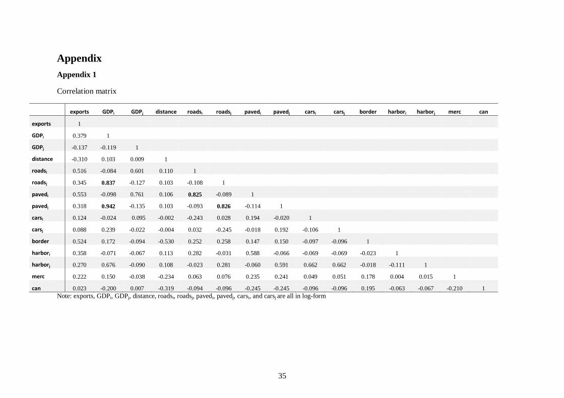
35

Appendix

Appendix 1

Correlation matrix

exports GDPi GDPj distance roadsi roadsj pavedi pavedj carsi carsj border harbori harborj merc can

exports 1

GDPi 0.379 1

GDPj -0.137 -0.119 1

distance -0.310 0.103 0.009 1

roadsi 0.516 -0.084 0.601 0.110 1

roadsj 0.345 0.837 -0.127 0.103 -0.108 1

pavedi 0.553 -0.098 0.761 0.106 0.825 -0.089 1

pavedj 0.318 0.942 -0.135 0.103 -0.093 0.826 -0.114 1

carsi 0.124 -0.024 0.095 -0.002 -0.243 0.028 0.194 -0.020 1

carsj 0.088 0.239 -0.022 -0.004 0.032 -0.245 -0.018 0.192 -0.106 1

border 0.524 0.172 -0.094 -0.530 0.252 0.258 0.147 0.150 -0.097 -0.096 1

harbori 0.358 -0.071 -0.067 0.113 0.282 -0.031 0.588 -0.066 -0.069 -0.069 -0.023 1

harborj 0.270 0.676 -0.090 0.108 -0.023 0.281 -0.060 0.591 0.662 0.662 -0.018 -0.111 1

merc 0.222 0.150 -0.038 -0.234 0.063 0.076 0.235 0.241 0.049 0.051 0.178 0.004 0.015 1

can 0.023 -0.200 0.007 -0.319 -0.094 -0.096 -0.245 -0.245 -0.096 -0.096 0.195 -0.063 -0.067 -0.210 1

Note: exports, GDPi, GDPj, distance, roadsi, roadsj, pavedi, pavedj, carsi, and carsj are all in log-form

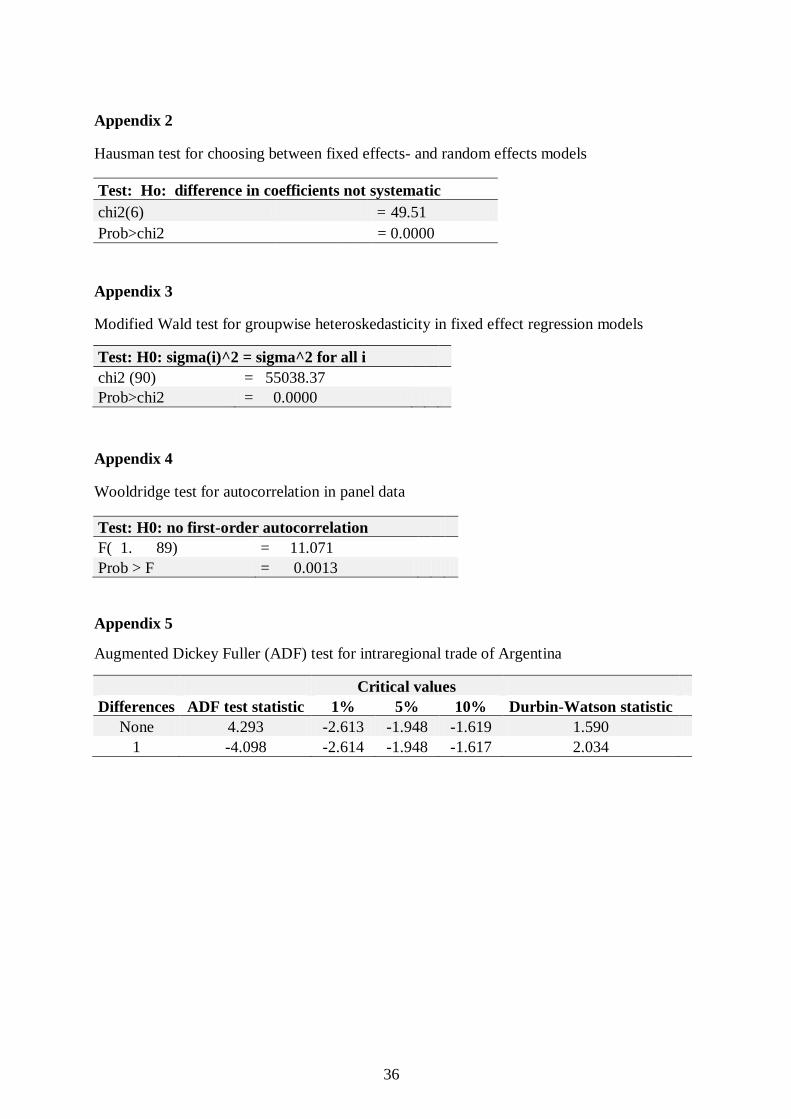
36

Appendix 2

Hausman test for choosing between fixed effects- and random effects models

Test: Ho: difference in coefficients not systematic

chi2(6)

= 49.51

Prob>chi2 = 0.0000

Appendix 3

Modified Wald test for groupwise heteroskedasticity in fixed effect regression models

Test: H0: sigma(i)^2 = sigma^2 for all i

chi2 (90) = 55038.37

Prob>chi2 = 0.0000

Appendix 4

Wooldridge test for autocorrelation in panel data

Test: H0: no first-order autocorrelation

F( 1. 89) = 11.071

Prob > F = 0.0013

Appendix 5

Augmented Dickey Fuller (ADF) test for intraregional trade of Argentina

Critical values

Differences ADF test statistic 1% 5% 10% Durbin-Watson statistic

None 4.293 -2.613 -1.948 -1.619 1.590

1 -4.098 -2.614 -1.948 -1.617 2.034

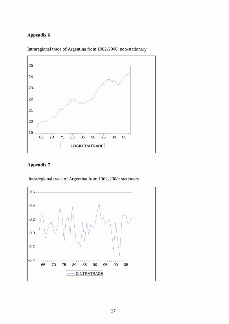
37

Appendix 6

Intraregional trade of Argentina from 1962-2008: non-stationary

Appendix 7

Intraregional trade of Argentina from 1962-2008: stationary

-0.4

-0.2

0.0

0.2

0.4

0.6

65 70 75 80 85 90 95 00 05

DINTRATRADE

19

20

21

22

23

24

25

65 70 75 80 85 90 95 00 05

LOGINTRATRADE