ORIGINAL PAPER Open Access

Transport indicator analysis andcomparison of 151 urban areas, based onopen source dataAli Enes Dingil1* , Joerg Schweizer2, Federico Rupi2 and Zaneta Stasiskiene1

Abstract

Introduction: The accurate analysis and comparison of transport indicators from a large variety of urban areas canhelp to evaluate the performance of different adopted transport policies. This paper attempts to determineimportant transport and socio-economic indicators from 151 urban areas and 51 countries, based on comparable,directly observable open-source data such as OpenstreetMap (OSM) and the TomTom database.

Analysis: This is the first, systematic indicator-analysis using recent, open source data from different urban areasaround the world. The indicator road kilometers per person, sometimes cited as infrastructure accessibility iscalculated by processing OSM data. Information on congestion levels have been taken from the TomTom databaseand socio-economic data from various, publicly accessible databases. Relations between indicators are identifiedthrough correlations and regression models are calibrated, quantifying the relation between transport infrastructureand performance indicators. Three sub-categories of cities with different population sizes (small cities, large citiesand metropolises) are defined and studied individually. In addition, a qualitative analysis is performed, putting fivedifferent indicators into relation.

Results & Conclusions: The main results reconfirm previous findings but with a larger sample size and morecomparable data. Good correlation values between infrastructure accessibility, socio-economic indicators, andcongestion levels are demonstrated. It is shown that cities with higher GDP have generally built more infrastructurewhich in turn reduces their congestion levels. In particular, for cities with low population density (aboveapproximately 1500 inh. Per sq.km), more roads per inhabitant lead to lower congestion levels; cities with highpopulation density have in general lower congestion levels if the rail infrastructure per person ratio is high.Furthermore, these cities increasing railways per person is more effective in reducing congestions than increasingroad length per person.

Keywords: Infrastructure accessibility, Congestion, Open source data, OSM, TomTom, Transport policy, Population density

1 IntroductionWorldwide, 55% of the global population lives in urbanareas and the present urban population is projected toincrease from today’s 4 billion people to 6 billion by 2050[48]. Mainly as a result of migration from rural areas, cit-ies are growing in terms of inhabitants and urban areaand form new residential areas outside or further awayfrom the city core. However, the speed of urbanizationpresents challenges such as meeting the growing demand

for transport infrastructure and affordable housing. Urbanzones take different forms and characterizations andurban growth patterns differ amongst regions as a resultof socio- economic, cultural, historical and environmentaldifferences. As an example, in the US, people tend to livein low-density, single-family houses and commute by carto work. In Japan by contrast, high-rise residential build-ings dominate and workers commute by public transpor-tation (mostly rail-based) [2]. In order to identify the mostpromising city development policy, it is of primary interestto assess the relations between network infrastructure,socio-economic indicators and the transport system per-formance based on experiences from existing cities; the

* Correspondence: ali.dingil@ktu.edu1Institute of Environmental Engineering, Kaunas University of Technology,Gedimino St. 50, LT-44239 Kaunas, LithuaniaFull list of author information is available at the end of the article

European TransportResearch Review

© The Author(s). 2019 Open Access This article is distributed under the terms of the Creative Commons Attribution 4.0International License (http://creativecommons.org/licenses/by/4.0/), which permits unrestricted use, distribution, andreproduction in any medium, provided you give appropriate credit to the original author(s) and the source, provide a link tothe Creative Commons license, and indicate if changes were made.

Dingil et al. European Transport Research Review (2018) 10:58 https://doi.org/10.1186/s12544-018-0334-4

understanding how cities are shaped by setting the appro-priate transport priorities can help to achieve terms of sus-tainable mobility objectives [36].The relationship between transport infrastructure expan-

sion and population growth, spatial expansion and land-usechange has been highlighted in many works [1, 5, 46]. Atight relationship between transport and urban develop-ment has been shown in earlier works [34, 37]. The imbal-ance between travel demand and transport infrastructuresupply as reason for the increase in congestion has beenstudied by Aljoufie et al. [1]. High congestion levels causesignificant costs to society; it has been estimated that expos-ure to traffic congestion reduces welfare in the US by $557million per year [17] and the estimation of congestion costto UK economy is approximately £13 billion per year, in aforecast through 2030 increasing to £21 billion per year[44]. Congestions impede the proper functioning of moresustainable transport modes such as bus services or cycling;as a consequence, existing bus services could neither meetthe growing transport demand, nor meet the demand ofthe cities’ economic development [45]. Due to these nega-tive impacts, congestion levels are a good candidate astransport performance indicator. More specific relations be-tween infrastructure expansion and various transport indi-cators have been found in the studies cited below.The expansion of road network generally leads to

lower population density in cities: Baum-Snow et al. [4]have shown that the integrated effects of ring roads andhighways in Chinese cities gave rise to move 25% of cen-tral inhabitants to surrounding zones. The empirical es-timates from Baum-Snow [3] show further that eachhighway expansion within an urban center of US me-tropolises causes an average 18% drop of inhabitants inthe city center. An analysis in Wisconsin within 1980–1990 demonstrated that highway expansions causedpopulation increase in suburban areas and booming theurban sprawl [13]. Similar results have been shown byanalyses in California between 1980 and 1994 [12]. Atthe contrary, rail network expansion has been shown toincrease population density at nearby urban rail stationsor tracks in several studies, thereby strengthening com-pactness of urban areas [6, 28, 31].The strong correlation between road infrastructure ex-

pansion and growth of vehicle ownership has been de-termined for 50 countries and 35 cities [26]. A positiverelationship between highway expansion and car usagehas been shown between 1982 and 2009 in the US [32].A negative correlation between transit ridership andhighways length has been found for the Montreal Region[15]. A sharp rise in car ownership in cities with lowrailway intensity and on the other hand a relatively slowrise of car ownership in cities with high railway intensityhave been shown for six Asian megacities located inChina, Japan and Thailand [27]. US cities with rail lines

experienced larger declines in car usage than cities withoutrail infrastructure between 2000 and 2009 [25]. Similarmodal shifts have been shown to exist in Europe: averagedover 14 LRT systems, approximately 11% of car drivers havechanged to rail [24]. With growing concerns over trafficcongestion and pollution from motorized vehicles, Dill andCarr [18] have indicated a positive correlation betweenbicycle usage and bicycle infrastructure expansion in43 US cities based on data from Bureau of the Cen-sus. This finding has been confirmed and quantifiedbased on a survey from 13 European cities [40].In summary, an extension of the road network tends

to decrease urban population density, decrease the ef-fectiveness of road based public transport -- conditionsfor favoring an increase in car ownership. A conse-quence of these effects is a further increase in privateroad transport demand which is often cited as “induceddemand” [30]. Rail and bike networks have been shownto achieve de-congesting effects.The choice of suitable and relevant indicators for the

analysis of transport policies is not obvious. Different defi-nitions of “accessibility” have been used as indicators.Geurs and Van Eck [22] has described various compo-nents of “accessibility”: land-use, temporal, individual andtransport. In an extensive review, Geurs and Wee [23]identified four types of possible accessibility measures:infrastructure-based, location-based, activity-based andutility-based accessibility.Based on these findings and conditioned by the avail-

ability of accessible data, this study will use the length oftransport infrastructure per person to quantify theamount of available transport infrastructure. This termis known as infrastructure accessibility [21]. The trans-port performance is quantified by congestion levels.The aim of the present study is to shed more light on

relations between transport-socio-economic indicatorsand transport performance indicators. The used data isthought to be comparable across all selected cities, allow-ing an absolute global evaluation of the transport perform-ance indicator. With respect to previous studies, thenumber of comparable cities is larger and more recent.Concrete transport policies are addressed by answeringthis question: under which conditions do more railwaysand bicycle infrastructure reduce congestion levels?The next section motivates the data collection for this

work and explains the principle data processing steps.The analysis and results are presented and discussed inAnalysis and results section, while the conclusions inSec. 4 summarizes the main findings.

2 Data collection and processingThe general approach of this work is to collect, process,correlate and model publicly available and comparabledata from a large number of cities around the world. In

Dingil et al. European Transport Research Review (2018) 10:58 Page 2 of 9

this section, all indicators are defined and the differentdata sources are described.

2.1 Socio-economic data-collection of citiesSocio-economic data has been sampled from a variety ofregions around the world -- data from 151 cities whichare distributed over 51 countries. Data of at least twoconsecutive population census as well as administrativespatial area information of urban areas were extractedfrom City population [16]. Population estimations areused in case local census data have not been available.Recent data of GDP per capita for each urban area havebeen sourced from the Organization for EconomicCo-operation and Development (OECD) database [38].All GDP values are expressed in American dollars, withan average value of the years 2010–2014. The missingOECD data has been completed from differencesources [8, 14, 20, 33, 41, 43]. The GDP per capita datais available for 139 cities. Population density is calculatedas population per spatial area in sq. km. Errors mayoccur by mixing GDP data from the OECD databasewith data from other sources. This error type concernspredominantly smaller cities. A general error source isthat urban boundary definitions of urban areas are notunified and that GDP data stems from different years.Both issues can lead to compatibility problems with theother data (performance and infrastructure indicators).

2.2 Performance indicator dataThe central performance indicator used for this study isthe congestion level in terms of average daily extra traveltime (ADETT), which is the extra travel time in a daywith respect to the free-floating traffic scenario, averagedover all monitored traffic participants of a distinct urbanarea. Comparable data on congestion level are retriev-able through the Tomtom database. Tomtom is used bymore than 6 million connected GPS devices and trafficis monitored by many million GSM probes and millionsof government-owned road sensor [42]. As Tomtom’smethodology is sufficiently accurate and unified all overthe world, it is a suitable data source for the presentstudy. However, errors may occur for several reasons: theTomTom data is not produced by a representative selec-tion of the population; the special distribution may not behomogeneous; finally the coverage may differ from city tocity and may also differ from the urban boundaries foundin Socio-economic data-collection of cities section.

2.3 Infrastructure related indicators from citiesThe infrastructure accessibility (IA) is expressed as infra-structure length per inhabitant (in meter infrastructureper 10 inhabitants). The network infrastructure length isdetermined for each infrastructure-type of a city fromthe OSM database, using the OSMNx software package

[10, 11]. OSM is a crowed sourced, unified and publiclyavailable map of the world. OSM infrastructure datalooks trustworthy for many cities, although it still needssome improvements on micro-level details. The OSMdata quality seems sufficient for macro-level analyses.OSM consists of three basic components: nodes, waysand relations [39]. Each component has various charac-terizing attributes, called tags. For instance, the way tagscan be used to identify the type of infrastructure.The Python software package OSMnx extracts and

converts OSM network data of the desired location intoa directed transport graph (which is a graph object ofthe Python networkX package) and performs some topo-logical corrections and node clustering simplification.The links of the graph retain the tag information of theways. Clearly, it is possible to generate sub-graphs foreach transport infrastructure (ordinary roads, bikewayand rail). OSMnx does provide options to generate andanalyze each of the sub-graphs.The area of the retrieved transport graph can be specified

by providing the polygon surrounding the area or throughthe name of the city. In the latter case, the administrativeboundaries of the desired city is retrieved from Open-StreetMaps’ Nominatim database. In most cases, officialboundaries have been available on Nominatim and only inrare cases, manual boundaries have been defined. The sta-tistics module of the OSMnx has been used to determinethe length of each subgraph, e.g. road length, rail lengthand bikeway length. Finally the infrastructure accessibilityIA is determined for all infrastructure types using thepopulation data (see Sec. 2.1). BRT infrastructure length issourced from www.brtdata.org [9] and BRT IA is deter-mined in mm per 10 inhabitants. Errors of the infrastruc-ture data are due to the incomplete OSM network orwrongly specified road attributes by volunteercontributors.

3 Analysis and resultsIn this section different analysis are performed and theirresults are discussed.

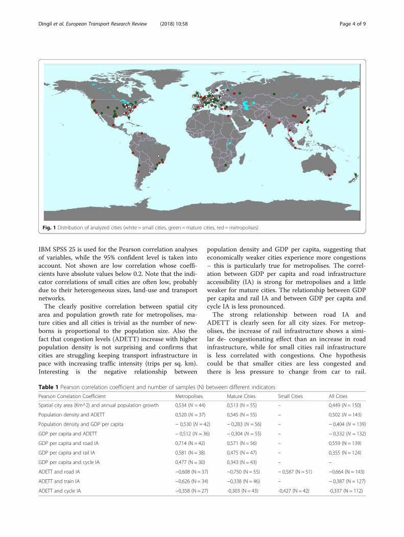
3.1 Correlations within city groupsIn order to render the city comparison more compar-able, cities are divided into three sub-groups, accordingto criteria explained in [19]: cities with a populationunder 800,000 are defined “small cities” (51 cities), citieswith a population between 800,000 and 3 million are de-fined “mature cities” (56 cities) and cities with a popula-tion over 3 million as are defined “metropolis” (44cities). The distribution of considered cities with respect-ive group-type is shown in the world map on Fig. 1.The Pearson Correlation Coefficient between different

indicators together with the number of samples areshown for different city sizes in Table 1. The software

Dingil et al. European Transport Research Review (2018) 10:58 Page 3 of 9

IBM SPSS 25 is used for the Pearson correlation analysesof variables, while the 95% confident level is taken intoaccount. Not shown are low correlation whose coeffi-cients have absolute values below 0.2. Note that the indi-cator correlations of small cities are often low, probablydue to their heterogeneous sizes, land-use and transportnetworks.The clearly positive correlation between spatial city

area and population growth rate for metropolises, ma-ture cities and all cities is trivial as the number of new-borns is proportional to the population size. Also thefact that congestion levels (ADETT) increase with higherpopulation density is not surprising and confirms thatcities are struggling keeping transport infrastructure inpace with increasing traffic intensity (trips per sq. km).Interesting is the negative relationship between

population density and GDP per capita, suggesting thateconomically weaker cities experience more congestions– this is particularly true for metropolises. The correl-ation between GDP per capita and road infrastructureaccessibility (IA) is strong for metropolises and a littleweaker for mature cities. The relationship between GDPper capita and rail IA and between GDP per capita andcycle IA is less pronounced.The strong relationship between road IA and

ADETT is clearly seen for all city sizes. For metrop-olises, the increase of rail infrastructure shows a simi-lar de- congestionating effect than an increase in roadinfrastructure, while for small cities rail infrastructureis less correlated with congestions. One hypothesiscould be that smaller cities are less congested andthere is less pressure to change from car to rail.

Fig. 1 Distribution of analyzed cities (white = small cities, green =mature cities, red =metropolises)

Table 1 Pearson correlation coefficient and number of samples (N) between different indicators

Pearson Correlation Coefficient Metropolises Mature Cities Small Cities All Cities

Spatial city area (Km^2) and annual population growth 0,534 (N = 44) 0,513 (N = 55) – 0,449 (N = 150)

Population density and ADETT 0,520 (N = 37) 0,545 (N = 55) – 0,502 (N = 143)

Population density and GDP per capita − 0,530 (N = 42) − 0,283 (N = 56) – − 0,404 (N = 139)

GDP per capita and ADETT − 0,512 (N = 36) − 0,304 (N = 55) – − 0,332 (N = 132)

GDP per capita and road IA 0,714 (N = 42) 0,571 (N = 56) – 0,559 (N = 139)

GDP per capita and rail IA 0,581 (N = 38) 0,475 (N = 47) – 0,355 (N = 124)

GDP per capita and cycle IA 0,477 (N = 30) 0,343 (N = 43) – –

ADETT and road IA −0,608 (N = 37) −0,750 (N = 55) − 0,587 (N = 51) −0,664 (N = 143)

ADETT and train IA −0,626 (N = 34) −0,338 (N = 46) – − 0,387 (N = 127)

ADETT and cycle IA −0,358 (N = 27) -0,303 (N = 43) -0,427 (N = 42) -0,337 (N = 112)

Dingil et al. European Transport Research Review (2018) 10:58 Page 4 of 9

These results confirm the previously mentioned find-ing that rail infrastructure has a relaxation effect onroad traffic for metropolises [7, 29, 47], presumablyby shifting car trips to rail trips. Combining the rela-tions between road/rail IA, congestions and GDP percapita, it could be hypothesized that economicallystrong metropolises can afford to expand road, railand bicycle infrastructure and are more successful inreducing congestions.

3.2 Statistical modelsAs IA and ADETT are generally well correlated, somestatistical models have been calibrated with the entire setof cities as well as on specific subsets. The best fit betweenroad infrastructure accessibility RIA and ADETT of all cit-ies is achieved with an exponential function of the shape:

ADETT ¼ a exp b RIAð Þ ð1ÞHowever, the fitting errors with a linear model are

only slightly superior. The results of this calibration isshown in Table 2. Despite the high noise levels in thedata, the coefficient b is negative, which means decreas-ing congestions with increasing road IA. This model hasbeen applied for the three city sub-groups and plottedtogether with the data points in Figs. 2, 3, 4.A further model is build which includes both, road in-

frastructure accessibility RIA and train infrastructure ac-cessibility TIA:

ADETT ¼ cþ d RIAþ e TIA ð2ÞAs RIA and TIA have the same unit, the coefficients d

and e quantify the reduction in traffic-congestions dueto an increase/decrease in road infrastructure or traininfrastructure, respectively. The interesting question ishow the coefficients d and e behave in cities with high andlow population densities. Table 3 shows the calibration re-sults of coefficients d and e for cities with a highpopulation density (above 1500 per sq. km) whileTable 4 shows the same calibration for cities with lowpopulation density (below 1500 per sq. km). The

Table 2 Calibration results of exponential function model Eq.(1)for all cities. R2 = 0.515, sample size N = 147

Calibration results Coef Std Err t P > |t| [95.0% Conf. Int.]

Log(a) 3.7734 0.037 100.773 0.000 3.699 3.847

b −0.0101 0.001 −12.232 0.000 −0.012 − 0.009

Fig. 2 Multi variant diagram of metropolises. Congestion level (ADETT) over Road IA; Bubble size is proportional to the population density; filledcolor indicates Train IA, bubble border color indicates Cycle IA, color of starred city- labels indicate BRT IA. For color scaling, see Table.5. Thedotted line represents the fitted exponential curve from Eq.(1)

Dingil et al. European Transport Research Review (2018) 10:58 Page 5 of 9

population density division at 1500 per sq. km hasbeen chosen arbitrarily. The main idea has been toisolate extreme space oriented cities in the US andAustralia. However, the division at 1500 per sq. kmcan be varied in reasonable bounds without changingthe core message of the results, as detailed below.The results for high density in Table 3 show that e

is significantly more negative than d (four times morenegative) and that both coefficients are significant.This result means that an increase in train infrastruc-ture per person reduces more congestion than the in-crease in road infrastructure per person. One reasonwhy rail lines combat congestion more effectively isprobably due to the fact that rail infrastructure hasbeen implemented primarily along the most congestedcorridors of the city. Therefore, the result of themodel does not mean that extending rail network be-yond the main traffic corridors will continue to re-duce traffic congestion.The situation for low density cities, shown in Table 4,

is less clear: e is only slightly more negative than d and eis statistically not significant (high P value). This means

railway building for low density cities appears less effect-ive in reducing congestions with respect to cities withhigh density cities.

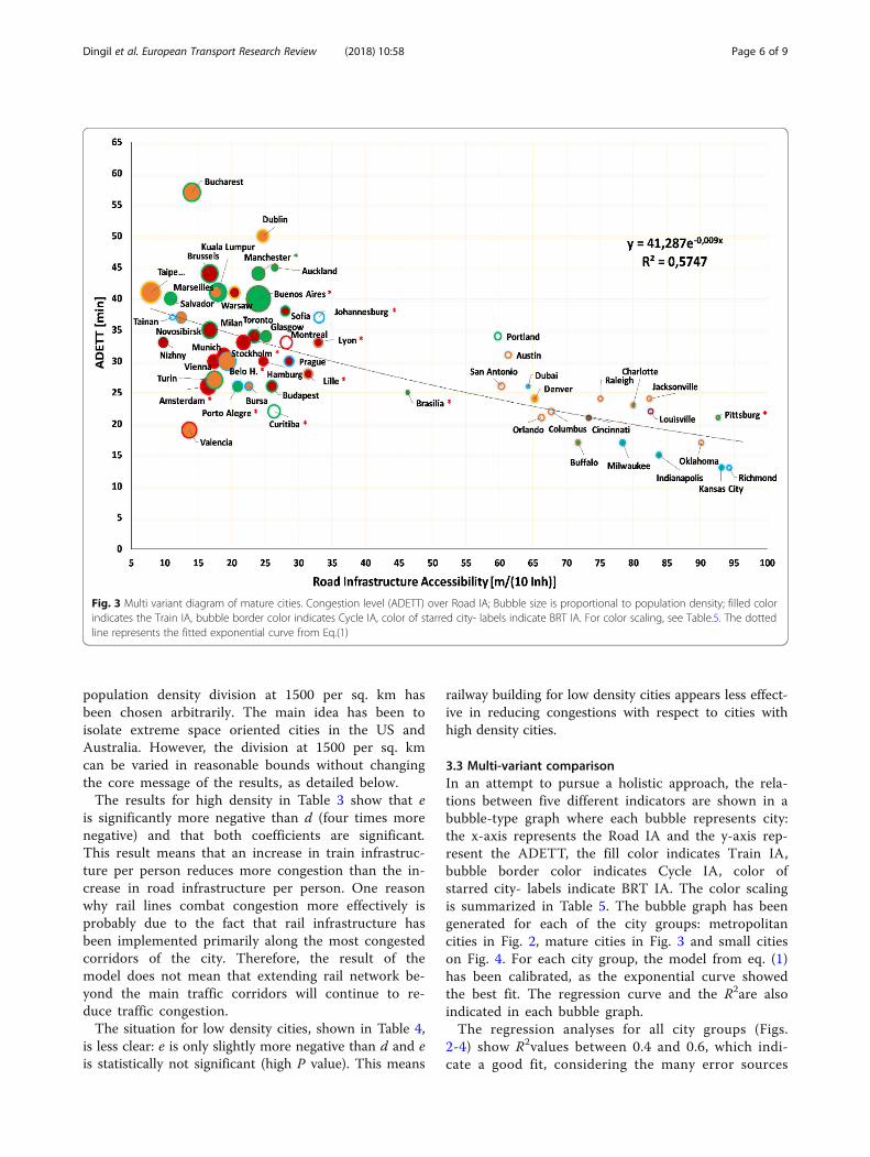
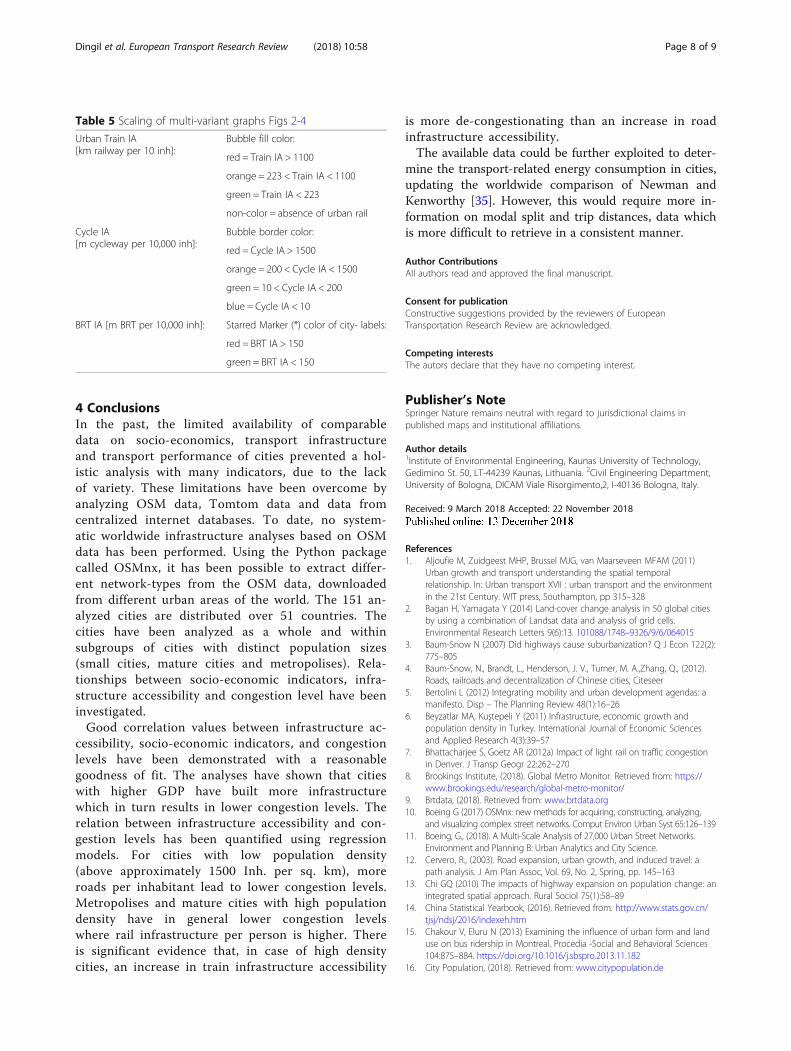
3.3 Multi-variant comparisonIn an attempt to pursue a holistic approach, the rela-tions between five different indicators are shown in abubble-type graph where each bubble represents city:the x-axis represents the Road IA and the y-axis rep-resent the ADETT, the fill color indicates Train IA,bubble border color indicates Cycle IA, color ofstarred city- labels indicate BRT IA. The color scalingis summarized in Table 5. The bubble graph has beengenerated for each of the city groups: metropolitancities in Fig. 2, mature cities in Fig. 3 and small citieson Fig. 4. For each city group, the model from eq. (1)has been calibrated, as the exponential curve showedthe best fit. The regression curve and the R2are alsoindicated in each bubble graph.The regression analyses for all city groups (Figs.

2-4) show R2values between 0.4 and 0.6, which indi-cate a good fit, considering the many error sources

Fig. 3 Multi variant diagram of mature cities. Congestion level (ADETT) over Road IA; Bubble size is proportional to population density; filled colorindicates the Train IA, bubble border color indicates Cycle IA, color of starred city- labels indicate BRT IA. For color scaling, see Table.5. The dottedline represents the fitted exponential curve from Eq.(1)

Dingil et al. European Transport Research Review (2018) 10:58 Page 6 of 9

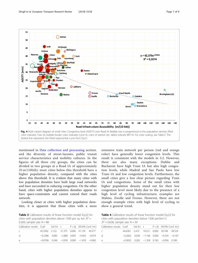
mentioned in Data collection and processing section.and the diversity of street-layouts, public transitservice characteristics and mobility cultures. In thefigures of all three city groups, the cities can bedivided in two groups at a Road IA of approximately35 m/(10Inh): most cities below this threshold have ahigher population density, compared with the citiesabove this threshold. It is evident that many cities withlow population densities have built large road networksand have succeeded in reducing congestion. On the otherhand, cities with higher population densities appear tohave space-constraints and cannot extend their roadsnetwork.Looking closer at cities with higher population dens-

ities, it is apparent that those cities with a more

extensive train network per person (red and orangecolor) have generally lower congestion levels. Thisresult is consistent with the models in 3.2. However,there are also many exceptions: Dublin andBucharest have high Train IA but also high conges-tion levels, while Madrid and Sao Paolo have lowTrain IA and low congestion levels. Furthermore, thesmall cities give a less clear picture regarding TrainIA and congestions. Some of the small cities withhigher population density stand out for their lowcongestion level most likely due to the presence of ahigh level of cycling infrastructure; examples areMalmo, Zwolle and Fresno. However, there are notenough example cities with high level of cycling toshow a general trend.

Table 4 Calibration results of linear function model Eq.(2) forcities with population densities below 1500 per/km^2.R2 = 0.638, sample size N = 39

Calibration results Coef Std Err t P > |t| [95.0% Conf. Int.]

c 44.6361 2.410 18.521 0.000 39.748 49.524

d −0.2602 0.036 −7.166 0.000 −0.334 −0.187

e −0.3835 0.282 −1.358 0.183 −0.956 0.189

Fig. 4 Multi variant diagram of small cities. Congestion level (ADETT) over Road IA; Bubble size is proportional to the population density; filledcolor indicates Train IA, bubble border color indicates Cycle IA, color of starred city- labels indicate BRT IA. For color scaling, see Table.5. Thedotted line represents the fitted exponential curve from Eq.(1)

Table 3 Calibration results of linear function model Eq.(2) forcities with population densities above 1500 per sq. km. R2 =0.269, sample size N = 88

Calibration results Coef Std Err t P > |t| [95.0% Conf. Int.]

c 45.3582 2.122 21.375 0.000 41.139 49.577

d −0.2386 0.083 −2.880 0.005 −0.403 −0.074

e −0.9706 0.246 −3.950 0.000 −1.459 −0.482

Dingil et al. European Transport Research Review (2018) 10:58 Page 7 of 9

4 ConclusionsIn the past, the limited availability of comparabledata on socio-economics, transport infrastructureand transport performance of cities prevented a hol-istic analysis with many indicators, due to the lackof variety. These limitations have been overcome byanalyzing OSM data, Tomtom data and data fromcentralized internet databases. To date, no system-atic worldwide infrastructure analyses based on OSMdata has been performed. Using the Python packagecalled OSMnx, it has been possible to extract differ-ent network-types from the OSM data, downloadedfrom different urban areas of the world. The 151 an-alyzed cities are distributed over 51 countries. Thecities have been analyzed as a whole and withinsubgroups of cities with distinct population sizes(small cities, mature cities and metropolises). Rela-tionships between socio-economic indicators, infra-structure accessibility and congestion level have beeninvestigated.Good correlation values between infrastructure ac-

cessibility, socio-economic indicators, and congestionlevels have been demonstrated with a reasonablegoodness of fit. The analyses have shown that citieswith higher GDP have built more infrastructurewhich in turn results in lower congestion levels. Therelation between infrastructure accessibility and con-gestion levels has been quantified using regressionmodels. For cities with low population density(above approximately 1500 Inh. per sq. km), moreroads per inhabitant lead to lower congestion levels.Metropolises and mature cities with high populationdensity have in general lower congestion levelswhere rail infrastructure per person is higher. Thereis significant evidence that, in case of high densitycities, an increase in train infrastructure accessibility

is more de-congestionating than an increase in roadinfrastructure accessibility.The available data could be further exploited to deter-

mine the transport-related energy consumption in cities,updating the worldwide comparison of Newman andKenworthy [35]. However, this would require more in-formation on modal split and trip distances, data whichis more difficult to retrieve in a consistent manner.

Author ContributionsAll authors read and approved the final manuscript.

Consent for publicationConstructive suggestions provided by the reviewers of EuropeanTransportation Research Review are acknowledged.

Competing interestsThe autors declare that they have no competing interest.

Publisher’s NoteSpringer Nature remains neutral with regard to jurisdictional claims inpublished maps and institutional affiliations.

Author details1Institute of Environmental Engineering, Kaunas University of Technology,Gedimino St. 50, LT-44239 Kaunas, Lithuania. 2Civil Engineering Department,University of Bologna, DICAM Viale Risorgimento,2, I-40136 Bologna, Italy.

Received: 9 March 2018 Accepted: 22 November 2018

References1. Aljoufie M, Zuidgeest MHP, Brussel MJG, van Maarseveen MFAM (2011)

Urban growth and transport understanding the spatial temporalrelationship. In: Urban transport XVII : urban transport and the environmentin the 21st Century. WIT press, Southampton, pp 315–328

2. Bagan H, Yamagata Y (2014) Land-cover change analysis in 50 global citiesby using a combination of Landsat data and analysis of grid cells.Environmental Research Letters 9(6):13. 101088/1748–9326/9/6/064015

3. Baum-Snow N (2007) Did highways cause suburbanization? Q J Econ 122(2):775–805

4. Baum-Snow, N., Brandt, L., Henderson, J. V., Turner, M. A.,Zhang, Q., (2012).Roads, railroads and decentralization of Chinese cities, Citeseer

5. Bertolini L (2012) Integrating mobility and urban development agendas: amanifesto. Disp – The Planning Review 48(1):16–26

6. Beyzatlar MA, Kuştepeli Y (2011) Infrastructure, economic growth andpopulation density in Turkey. International Journal of Economic Sciencesand Applied Research 4(3):39–57

7. Bhattacharjee S, Goetz AR (2012a) Impact of light rail on traffic congestionin Denver. J Transp Geogr 22:262–270

8. Brookings Institute, (2018). Global Metro Monitor. Retrieved from: https://www.brookings.edu/research/global-metro-monitor/

9. Brtdata, (2018). Retrieved from: www.brtdata.org10. Boeing G (2017) OSMnx: new methods for acquiring, constructing, analyzing,

and visualizing complex street networks. Comput Environ Urban Syst 65:126–13911. Boeing, G., (2018). A Multi-Scale Analysis of 27,000 Urban Street Networks.

Environment and Planning B: Urban Analytics and City Science.12. Cervero, R., (2003). Road expansion, urban growth, and induced travel: a

path analysis. J Am Plan Assoc, Vol. 69, No. 2, Spring, pp. 145–16313. Chi GQ (2010) The impacts of highway expansion on population change: an

integrated spatial approach. Rural Sociol 75(1):58–8914. China Statistical Yearbook, (2016). Retrieved from: http://www.stats.gov.cn/

tjsj/ndsj/2016/indexeh.htm15. Chakour V, Eluru N (2013) Examining the influence of urban form and land

use on bus ridership in Montreal. Procedia -Social and Behavioral Sciences104:875–884. https://doi.org/10.1016/j.sbspro.2013.11.182

16. City Population, (2018). Retrieved from: www.citypopulation.de

Table 5 Scaling of multi-variant graphs Figs 2-4

Urban Train IA[km railway per 10 inh]:

Bubble fill color:

red = Train IA > 1100

orange = 223 < Train IA < 1100

green = Train IA < 223

non-color = absence of urban rail

Cycle IA[m cycleway per 10,000 inh]:

Bubble border color:

red = Cycle IA > 1500

orange = 200 < Cycle IA < 1500

green = 10 < Cycle IA < 200

blue = Cycle IA < 10

BRT IA [m BRT per 10,000 inh]: Starred Marker (*) color of city- labels:

red = BRT IA > 150

green = BRT IA < 150

Dingil et al. European Transport Research Review (2018) 10:58 Page 8 of 9

17. Currie J, Walker R (2011) Traffic congestion and infant health: evidence frome-zpass. Am Econ J Appl Econ 3(1):65–90, 2011

18. Dill J, Carr T (2003) Bicycle commuting and facilities in major U.S. cities: ifyou build them, commuters will use them. Transp Res Rec 1828:116–123

19. Doxiades KA (1968) Ekistics: an introduction to the science of humansettlements. Hutchinson, London

20. Eurostat, (2018). Regional gross domestic product (PPS per inhabitant) byNUTS 2 regions. Retrieved from: http://ec.europa.eu/eurostat/tgm/refreshTableAction.do?tab=table&plugin=1&pcode=tgs00005&language=en

21. European Environment Agency (2018). Infrastructure density andaccessibility by country, https://www.eea.europa.eu/data-and-maps/daviz/infrastructure-density-and-accessibility-per-country-1

22. Geurs KT, Ritsema van Eck JR (2001) Accessibility measures: review andapplications. RIVM report 408505 006, National Institute of Public Health andthe Environment, Bilthoven Available at: www.rivm.nl/bibliotheek/rapporten/408505006.html

23. Geurs KT, van Wee B (2004) Accessibility evaluation of land-use andtransport strategies: review and research directions. J Transp Geogr 12(2):127–140

24. Hass-Klau C, Crampton G, Biereth C, Deutsch V (2004) Bus or light rail:Making the right choice: A financial, operational, and demand comparisonof light rail, guided busways and bus lanes. Environmental & TransportPlanning, Brighton and Government of United Kingdom

25. Henry, L. and Litman T., (2014). Evaluating new start transit programperformance: comparing rail and bus. Victoria Transport Policy Institute

26. Ingram, G. and Z. Liu, (1999). Determinants of motorization and roadprovision. In Gomez Ibanez et al. (ed.), Essays in Transportation Economicsand Policy, Brookings Institution Press, pp. 325–356

27. Ito K, Nakamura K, Kato H, Hayashi Y (2013) Influence of urban railwaydevelopment timing on long-term car ownership growth in asiandeveloping mega-cities. J. East. Asia Soc. Transp Stud 10:1076–1085

28. Levinson D (2008) Density and dispersion: the co-development of landuse and rail in London. J Econ Geogr 8(1):55–77. https://doi.org/10.1093/Jeg/Lbm038

29. Litman T (2005) “Impacts of rail transit on the performance of atransportation system” Transportation Research Record 1930. TransportationResearch Board 2005:23–29. www.trb.org

30. Litman T (2018) Generated Traffic: Implications for Transport Planning.Report. In: Victoria transport policy institute

31. McMillen DP, Lester TW (2003) Evolving subcenters: employment andpopulation densities in Chicago, 1970–2020. J Hous Econ 12(1):60–81.https://doi.org/10.1016/S1051-1377(03)00005-6

32. Melo P S, Graham D J, Canavan S., (2012). Effects of road investments oneconomic output and induced travel demand evidence for urbanized areasin the United States, Transp Res Rec, vol. 2297 (pg. 163–171)

33. National Human Development Report for the Russian Federation, (2011).Modernization and Human Development. Retrieved from: http://www.undp.ru/documents/nhdr2011eng.pdf

34. Newman P, Kenworthy JR (1996) The land use-transport connection: Anoverview. Land Use Policy 13(1):1–22

35. Newman P, Kenworthy J (1988) The transport energy trade-off: fuel-efficienttraffic versus fuel-efficient cities. Transportation Research Part A: General22(3):163–174

36. Newman, P., (2015), “Transport infrastructure and sustainability: a newplanning and assessment framework”, Vol 4 Issue: 2, pp.140–153, https://doi.org/10.1108/SASBE-05-2015-0009

37. Muller P (2004) Transportation and Urban Form: Stages in the SpatialEvolution of the American Metropolis. The Geography of UrbanTransportation, Guilford Publications, pp 59–85

38. OECD, (2018). Regions and cities database. Retrieved from OECD: https://stats.oecd.org/Index.aspx?DataSetCode=CITIES

39. Openstreetmap (OSM), (2018). Retrieved from: https://wiki.openstreetmap.org/wiki/Tags

40. Schweizer J, Rupi F (2013) Performance evaluation of extreme bicycle scenarios.Procedia - Social and Behavioral Sciences 111:508–517 ISSN 1877-0428

41. Stats NZ (2016) Urban. Development Retrieved from: https://www.stats.govt.nz/42. Tomtom, (2018). Real time & historical traffic: TomTom delivers a unique

proposition. Retrieved from Tomtom: https://www.tomtom.com/lib/doc/licensing/RTTHT.EN.pdf

43. Turkish Statistical Institute, (2014). Retrieved from : http://www.turkstat.gov.tr/PreTabloArama.do?metod=search&araType=vt

44. Urban Transportation Group, (2018). Rail cities UK: our vision for their future.Report Retrieved from: http://www.urbantransportgroup.org/resources/types/reports/rail-cities-uk-our-vision-their-future

45. Yang Y., Zhang P., Ni S., (2014). Assessment of the Impacts of Urban RailTransit on Metropolitan Regions Using System Dynamics Model.Transportation research Procedia. T 4 – S. 521–534

46. Wegener M, Fürst F (1999) Land-use transport interaction: State of the art.Project TRANSLAND (integration of transport and land use planning). In:University of Dortmund

47. Winston C, Langer A (2006) The effect of government highway spending onroad users’ congestion costs. J Urban Econ 60(3):463–483

48. Worldbank, (2018). Urban Development Overview. Retrieved from : http://www.worldbank.org/en/topic/urbandevelopment/overview

Dingil et al. European Transport Research Review (2018) 10:58 Page 9 of 9