Transport in Dynamical Astronomy and Multibody … › ... › papers › DeJuKoLeLoMaPaPrRoTh2005.pdfTransport in Dynamical Astronomy and Multibody Problems Michael Dellnitz∗, Oliver

Transport in Dynamical Astronomy

and Multibody Problems

Michael Dellnitz∗, Oliver Junge∗, Wang Sang Koon†, Francois Lekien‡,Martin W. Lo§, Jerrold E. Marsden†, Kathrin Padberg∗, Robert Preis∗,

Shane D. Ross†, Bianca Thiere∗

International Journal of Bifurcation and Chaos 15, 699–727, 2005

Abstract

We combine the techniques of almost invariant sets (using tree structuredbox elimination and graph partitioning algorithms) with invariant manifoldand lobe dynamics techniques. The result is a new computational technique forcomputing key dynamical features, including almost invariant sets, resonanceregions as well as transport rates and bottlenecks between regions in dynamicalsystems. This methodology can be applied to a variety of multibody problems,including those in molecular modeling, chemical reaction rates and dynamicalastronomy. In this paper we focus on problems in dynamical astronomy to illus-trate the power of the combination of these different numerical tools and theirapplicability. In particular, we compute transport rates between two resonanceregions for the three body system consisting of the Sun, Jupiter and a thirdbody (such as an asteroid). These resonance regions are appropriate for certaincomets and asteroids.

Key words. Three-body problem, transport rates, dynamical systems, almostinvariant sets, graph partitioning, set-oriented methods, invariant manifolds, lobedynamics

2000 AMS subject classification. 37M05, 37N05, 37M25

2001 PACS subject classification. 05.60.Cd, 95.10.Ce, 96.30.-t

∗Faculty of Computer Science, Electrical Engineering and Mathematics, University of Paderborn,D-33095 Paderborn, Germany

†Control and Dynamical Systems, MC 107-81, California Institute of Technology, Pasadena, CA91125, USA.

‡Department of Mechanical and Aerospace Engineering, Princeton University Engineering Quad,Olden Street, Princeton, NJ 08544-5263, USA

§Navigation and Mission Design, Jet Propulsion Laboratory, California Institute of Technology,M/S 301-140L, 4800 Oak Grove Drive, Pasadena, CA 91109, USA.

1

Contents 2

Contents

1 Introduction 2

2 Description of the PCR3BP Global Dynamics 8

3 Computing Transport 93.1 Lobe Dynamics . . . . . . . . . . . . . . . . . . . . . . . . . . . . . . 103.2 Set Oriented Approach . . . . . . . . . . . . . . . . . . . . . . . . . . 14

4 Example: The Sun-Jupiter-Asteroid System 234.1 Lobe Dynamics . . . . . . . . . . . . . . . . . . . . . . . . . . . . . . 234.2 Set Oriented Approach . . . . . . . . . . . . . . . . . . . . . . . . . . 26

5 Conclusions and Future Directions 33

1 Introduction

The mathematical description of transport phenomena applies to a wide rangeof physical systems across many scales (Meiss [1992]; Wiggins [1992]; Rom-Kedar[1999]). The recent and surprisingly effective application of methods combining dy-namical systems ideas with those from chemistry to the transport of Mars impactejecta underlines this point (Jaffe, Ross, Lo et al. [2002]). In this paper, we de-velop computational methods to study transport based on the relationship betweenstatistics and geometry in a nonlinear dynamical system with mixed regular andchaotic motion. Our focus is the transport of material throughout the solar system.However, these methods are fundamental and broad-based; they may be applied todiverse areas of study, including fluid mixing (Rom-Kedar, Leonard, and Wiggins[1990]; Malhotra and Wiggins [1998]; Poje and Haller [1999]; Coulliette and Wig-gins [2001]; Lekien, Coulliette, and Marsden [2003]), N -body problems in physicalchemistry (Jaffe, Farrelly, and Uzer [2000]; Lekien and Marsden [2004]) as well asother problems in dynamical astronomy. For example, the recent discovery of severalbinary pairs in the asteroid and Kuiper belts has stimulated interest in computingthe formation and dissociation rates of such binary pairs (see, for instance Goldre-ich, Lithwick, and Sari [2002]; Scheeres [2002]; Scheeres, Durda, and Geissler [2002];Veillet, Parker, Griffin, Marsden et al. [2002]).

Dynamical Processes in the Solar System. Our understanding of the solarsystem has changed dramatically in the past several decades with the realizationthat the orbits of the planets and some minor bodies are chaotic. In the case ofplanets, this chaos is of a sufficiently weak nature that their motion appears quiteregular on relatively short time scales (Laskar [1989]). In contrast, small bodies suchas asteroids, comets, and Kuiper-belt objects can exhibit strongly chaotic motionthrough their interactions with the planets and the Sun, exhibiting Lyapunov timesof only a few decades (Torbett and Smoluchowski [1990]; Tancredi [1995]).

1 Introduction 3

The ability to predict the behavior of populations of these small but numerousobjects is essential for understanding key transport phenomena in dynamical as-tronomy, such as the evolution of short period comets (Torbett and Smoluchowski[1990]), scattered Kuiper-belt objects (Malhotra, Duncan, and Levison [2000]), andthe intermediaries between these two populations (Tiscareno and Malhotra [2003]).Furthermore, an understanding of how small bodies behave in n-body fields will aidin the gravitationally assisted transport of spacecraft using very little fuel (Koon,Lo, Marsden, and Ross [2000, 2001a, 2002]; Gomez et al. [2001]; Dellnitz, Junge,Lo, and Thiere [2001]; Ross, Koon, Lo and Marsden [2003]; Yamato and Spencer[2003]). This understanding also contributes to other fields such as astrobiology, forexample, where comet impact rates are key for determining the delivery of waterto the Earth (Morbidelli et al. [2000]) and ejecta exchange rates are important forinvestigating the transportation of microbes between Mars and Earth (Gladman etal. [1996]; Mileikowsky et al. [2000]).

The recent discovery of several extrasolar planetary systems has stimulated in-terest in the morphological and dynamical features that may be present in genericplanetary systems (Konacki, Torres, Jha, and Sasselov [2003]). Some quantities ofinterest are the following: likely distributions of objects in the presence of dynamicalsculpting due to planets and moons (e.g., generic circumstellar belts and circumsolarrings); rates of small body collision with a planet; and rates of capture and escapefrom one orbital resonance with a planet to another.

Short Period Comets. In order to develop a theory of chaotic transport thatis computationally tractable, we will consider a physically relevant example fromdynamical astronomy: the motion of (short period) comets in the gravitationalfield of the Sun and Jupiter. Our model, the planar circular restricted three-bodyproblem (PCR3BP), will be described in a later Section.

The Role of the Planar Circular Restricted Three-Body Problem. ThePCR3BP has long been considered an appropriate “baseline” model for providinga reasonable explanation for much of the dynamical behavior found in the largescale numerical experiments of solar system dynamics (Levison and Duncan [1993];Malhotra, Duncan, and Levison [2000]). Malhotra’s work in Malhotra [1996] pro-vides a good recent example. Motivated by numerical studies of the stability oflow-eccentricity and low-inclination orbits of small bodies in the trans-NeptunianKuiper belt, Malhotra [1996] used the PCR3BP to describe the basic phase spacestructure in the neighborhood of Neptune’s exterior mean motion resonances. Theadvantage of this simple model is that it allows the direct visualization, in two-dimensional surfaces-of-section, of a global mixed phase space structure of stableand chaotic zones. Much can be learned about populations of minor bodies froma semi-analytical study of the PCR3BP, i.e., careful numerics guided by dynamicalsystems theory.

1 Introduction 4

Need for Modification of Current Transport Calculations

Several subjects make use of dynamical transport calculations. We indicate some ofthe reasons one would like to improve current techniques.

Chemistry. The transport of ensembles of points in phase space has been im-portant for the theoretical determination of chemical reaction rates. One method,transition state theory (TST), has been a ubiquitous workhorse in the computa-tional chemistry literature (Uzer, Jaffe, Palacian, Yanguas, and Wiggins [2002]).It is based on the identification of a transition state (TS) between large realms ofphase space which correspond to either “reactants” or “products.” If one assumesthe phase space in each realm is structureless (Marston and De Leon [1989]), thenthe chemical reaction rate for the reaction under study can be estimated from theflux through the TS. However, rates given by TST can be off of the true rate byorders of magnitude (De Leon [1992]). Modifications of transition state theory arenecessary to calculate statistical quantities of interest (Hammes-Schiffer and Tully[1995]; Hammes-Schiffer [2002]; Agarwal et al. [2002]).

Dynamical Astronomy. In principle, the computation of rates of mass transportcan be accomplished by numerical simulations in which the orbits of vast numbers oftest particles are propagated in time including as many gravitational interactions asdesirable. Many investigators have used this approach successfully (cf. Levison andDuncan [1993]). However, such calculations are computationally demanding and itmay be difficult to extract from them information about key dynamical mechanismssince the outcomes may depend sensitively on the initial conditions used for thesimulation or may even be misleading. To obtain general features of planetarysystem evolution and morphology, which is a major goal of dynamical astronomy,other approaches may be necessary.

Current Methods for the Study of Transport in the PCR3BP

Many of the important transport questions involve motion between different regionsof the phase space. There have been a variety of approaches to deal with thisquestion from various points of view. We recall some of them in this subsection.

Analytical Methods: Single Resonance Theory and Resonance OverlapCriterion. One approach is to develop simple analytical models which provideanswers to basic phase space transport questions. Much progress has been made inthis area, but most of the work has focused on the study of the local dynamics arounda single resonance, using a one-degree-of-freedom pendulum-like Hamiltonian withslowly varying parameters. Transport questions regarding capture into, and passagethrough resonance, have been addressed this way (Henrard [1982]; Neishtadt [1996];Neishtadt, Sidorenko, and Treschev [1997]).

An important result regarding the interaction between resonances was obtainedby Wisdom [1980], where the method of Chirikov [1979] was applied to the PCR3BP

1 Introduction 5

to determine a resonance overlap criterion for the onset of chaotic behavior for smallmass parameter (ε). These analytical methods are still used today (see Murray andHolman [2001] and references therein).

Toward a Global Picture of the Phase Space. In Koon, Lo, Marsden, andRoss [2000], dynamical systems techniques were applied to the problem of hetero-clinic connections and interior-exterior transitions in the PCR3BP, laying the foun-dation for tube dynamics. In the point of view developed in Koon, Lo, Marsden, andRoss [2000], the invariant manifold structures associated to L1 and L2, the (Conley-McGehee) phase space tubes (Conley [1968]; McGehee [1969]) play a key role. Thesetubes provide fundamental tools that can aid in understanding transport throughoutthe phase space, e.g., transport between the inside and outside of a planet’s orbit,as seen in the comet P/Oterma (Carusi, Kresak, Pozzi, and Valsecchi [1985]), andchaotic trajectories leading to planetary impact, as in comet D/Shoemaker–Levy 9(Benner and McKinnon [1995]).

The main new technical result in Koon, Lo, Marsden, and Ross [2000] is thenumerical demonstration of the existence of a heteroclinic connection between pairsof periodic orbits, one around the libration point L1 and the other around L2, withthe two periodic orbits having the same energy. This result is applied to the interior-exterior transition problem, providing insight into the “resonance hopping” of someshort period comets (cf. Tancredi, Lindgren, and Rickman [1990]; Valsecchi [1992];Belbruno and Marsden [1997]; Koon, Lo, Marsden, and Ross [2001]). Furthermore,an explicit numerical construction of interesting orbits with prescribed itineraries isdeveloped, based on ideas from a proof of global motion in the PCR3BP.

For particles in the PCR3BP with energy slightly greater than that of L2, theinterior, exterior and planetary realms are connected by bottlenecks about L1 andL2 (see Figure 2.1(c) in the next section). Particles can pass between realms onlythrough these bottlenecks by being inside phase space tubes, regions bounded bypieces of the stable and unstable invariant manifolds of periodic orbits around L1

and L2. We can determine the flux between realms by monitoring the flux throughthese tubes.

Mars Escape Rates. Building on the ideas described in the preceding paragraph,the rate of escape of particles temporarily captured by Mars was computed in Jaffe,Ross, Lo et al. [2002]; Ross [2003]. That paper uses a statistical assumption that iscommon in transition state theory in chemistry, and which is appropriate for thisproblem. Theory and direct Monte Carlo simulations are shown to agree to within1%, which showed the promise of a dynamical systems approach for the computationof interesting transport rates in dynamical astronomy.

The work of Rom-Kedar and Wiggins [1990], contains an investigation of thetransport in the two-dimensional phase space of Cr diffeomorphisms (r ≥ 1) of two-manifolds between regions of the phase space bounded by pieces of the stable andunstable manifolds of hyperbolic points. The transport mechanism is associated withthe dynamics of homoclinic and heteroclinic tangles, and the study of this dynamicsleads to a general formulation of the transport rates in terms of distributions of

1 Introduction 6

small phase space regions called “lobes.” By following the evolution of these lobes,lobe dynamics supplies a method for theoretically computing short and long termtransport rates. However, computational issues have limited its applications (Rom-Kedar and Wiggins [1990, 1991]; Meiss [1992]). Important contributions to thiseffort were made by Lichtenberg and Lieberman [1983]; MacKay, Meiss, and Percival[1984, 1987]; Meiss [1992]; Meiss and Ott [1986].

The manifolds computed in such problems are typically complicated because ofthe nature of homoclinic and heteroclinic tangles. Furthermore, the length of thesecomplicated curves grows quickly with the size of the time window of interest. Thenumber of points needed to describe long segments of manifolds can be prohibitivelylarge if naive computational methods are used. One also needs to take into accountthe fine structure of the lobes and manifolds, and in particular the effect of re-entrainment of the lobes, i.e., the implications of the lobes leaving and re-enteringthe specified regions on the transport rate. We show later on that this effect is infact, important in the three-body problem and cannot be ignored.

Recent efforts made to incorporate lobe dynamics into geophysical, fluid, andchemical transport calculations have brought new techniques to compute invariantmanifolds (see Coulliette and Wiggins [2001]; Lekien and Marsden [2004]; Lekien andCoulliette [2004]; Lekien, Coulliette, and Marsden [2003]). Using those techniques,one is able to compute very long segments of stable and unstable manifolds withhigh accuracy by conditioning the manifolds adaptively, for instance, by insertingmore points along the manifold where the curvature is high (see Hobson [1993];Lekien [2003]). As a result, the length and shape of the manifold is not an obstacleanymore and many more iterates of lobes than hitherto possible can be generatedaccurately. Using this approach, one keeps track of all the points throughout thecomputation, with the drawback that the resulting algorithms often require a greatdeal of memory. A related set of studies (You, Kostelich, and Yorke [1991]; Kostelich,Yorke, and You [1996]) describes a method for restricting the invariant manifoldcomputation to specific regions of interest, thereby using significantly less memory,while rigorously guaranteeing that the computed manifold lies no further than aspecified tolerance from the “true” manifold.

Set Oriented Approach to Transport

In contrast to the geometric approach to the analysis of transport phenomena asdescribed in the preceding paragraphs, the set oriented approach focuses on a globaldescription of the dynamics on a coarse level. To this end one considers a transferoperator associated to the underlying map. Roughly speaking, this operator de-scribes how some initial distribution evolves under the dynamics. Via a partitionof some interesting invariant part in phase space this operator can be discretized,yielding a stochastic matrix or, equivalently, a directed weighted graph, which maybe viewed as a coarse-grain model of the global dynamics.

Transport rates between subsets of phase space can easily be computed usingthis matrix of transition probabilities. When these subsets are given as unions ofpartition elements, the computed rates are exact. However, in general the accuracy

1 Introduction 7

of the computed quantities is determined by the size of the partition elements.In addition to computing transport rates it is also possible to obtain insight

about what “important” or interesting regions in phase space might be. The ideais that the transfer operator encodes a macroscopic description of the dynamics.One way to reveal this information is to consider the corresponding graph, to whichstandard algorithms from graph theory can directly be applied for a further analysis.For example, we use algorithms for graph partitioning (see e.g. software-librariessuch as chaco (Hendrickson and Leland [1995]), jostle (Walshaw [2000]), metis(Karypis and Kumar [1999]), scotch (Pellegrini [1996]) or party (Monien, Preisand Diekmann [2000])) to find regions that are determined by (i) a high transportrate within the region and (ii) a small transport rate to other regions. In terms ofdynamical systems, these sets are referred to as almost invariant sets (Dellnitz andJunge [1999]). In particular, we use the Party library with extensions, which areexplicitly developed for the analysis of almost invariant sets in dynamical systems(Dellnitz and Preis [2003]). A key observation of this paper is that regions that wecompute by this approach are actually those bounded by certain invariant manifolds.

What is Achieved in this Paper

The main results of this paper are

• Further development of the basic theory and application of computationaltechniques for transport. In particular, a comparison as well as a synthesisof tools from lobe dynamics and set oriented methods is presented. Errorestimates are provided, which show, in particular, the convergence of the set-oriented methods.

• In regimes where the comparison makes sense, it is shown that the agreementis very good on a sample problem. Based on the initial information providedby the combination of the two methods, the set oriented methods are able tocarry out many more iterates than heretofore possible.

• As a concrete nontrivial example illustrating the methods, the transport ratefrom an interesting resonant region R1 to a surrounding region R2 in the Sun-Jupiter system, exterior to the orbit of Jupiter and at a particular energyvalue, are computed. It is computed that the probability (in the sense of thefractional area) that a transition from R1 to R2 occurs is about 28% in aperiod of about 1817 Earth years.

• The methods of this paper lay the foundation for many other computationsof astrodynamical interest. In particular, in Dellnitz, Junge, Lo, et. al. [2005]we study the transport rate of asteroids from the Hilda region to a regiondefined by crossers of Mars’ orbit as well as a remarkable relation betweenalmost invariant sets associated with the Sun-Jupiter three body system andthe orbits of all the planets interior to Jupiter.

2 Description of the PCR3BP Global Dynamics 8

2 Description of the PCR3BP Global Dynamics

Problem Description. The PCR3BP is a particular case of the general gravi-tational problem of three masses m1,m2,m3 defined by the following restrictions:(a) the motion of all three bodies takes place in a common plane; (b) the massesm1 and m2 move on circular orbits about their common center of mass; and (c) thethird body, m3, has zero mass; therefore it does not influence the motion of m1 andm2. In the context of this paper, m1 represents the Sun and m2 represents a planet,and we are concerned with the motion of the third body, the test particle m3. Thesystem is made nondimensional by the following choice of units: the unit of mass istaken to be m1 + m2; the unit of length is chosen to be aP the constant separationbetween m1 and m2 (i.e., the mean separation of the Sun and planet); the unit oftime is chosen such that the orbital period of m1 and m2 about their center of massis 2π. Then the universal constant of gravitation, G = 1, and the masses of the Sunand planet are 1− ε and ε, where ε = m2/(m1 + m2).

Equations of Motion. Choosing a rotating coordinate system so that the originis at the center of mass, the Sun and planet are on the x-axis at the points (−ε, 0)and (1 − ε, 0) respectively. Let (x, y) be the position of the particle in the plane,then the equations of motion for the particle in this rotating frame are:

x− 2y = −Ux y + 2x = −Uy, (2.1)

where

U = −x2 + y2

2− 1− ε

rS− ε

rP− ε(1− ε)

2.

Here, the subscripts of U denote partial differentiation in the respective variable,and rS , rP are the distances from the particle to the Sun and planet respectively.See Szebehely [1967] for more details on the derivation of this equation and Koon,Marsden, Ross, Lo, and Scheeres [2004] for its derivation using Lagrangian mechan-ics .

Energy Manifolds. Equations (2.1) are autonomous and are in Euler–Lagrangeform (and thus, using the Legendre transformation, can be put into Hamiltonianform as well). They have an energy integral

E =12(x2 + y2) + U(x, y), (2.2)

which is related to the Jacobi constant C by C = −2E. The motion of the testparticle takes place on a 3-dimensional energy manifold (defined by a particularvalue of E) embedded in the 4-dimensional phase space, (x, y, x, y).

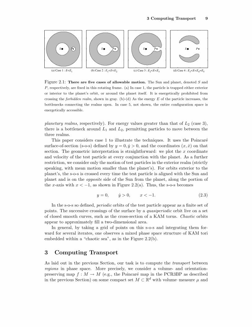
The value of the energy is an indicator of the type of global dynamics possible fora particle in the PCR3BP, which can be broken down into five cases (see Figure 2.1).In case 1, shown in Figure 2.1(a), the particle is trapped either exterior or interiorto the planet’s orbit, or around the planet itself (labeled the exterior, interior, and

3 Computing Transport 9

S P

(a) Case 1 : E<E1

S P

(b) Case 2 : E1<E<E2

S P

(d) Case 4 : E3<E<E4=E5

S P

(c) Case 3 : E2<E<E3

Figure 2.1: There are five cases of allowable motion. The Sun and planet, denoted S and

P , respectively, are fixed in this rotating frame. (a) In case 1, the particle is trapped either exterior

or interior to the planet’s orbit, or around the planet itself. It is energetically prohibited from

crossing the forbidden realm, shown in gray. (b)-(d) As the energy E of the particle increases, the

bottlenecks connecting the realms open. In case 5, not shown, the entire configuration space is

energetically accessible.

planetary realms, respectively). For energy values greater than that of L2 (case 3),there is a bottleneck around L1 and L2, permitting particles to move between thethree realms.

This paper considers case 1 to illustrate the techniques. It uses the Poincaresurface-of-section (s-o-s) defined by y = 0, y > 0, and the coordinates (x, x) on thatsection. The geometric interpretation is straightforward: we plot the x coordinateand velocity of the test particle at every conjunction with the planet. As a furtherrestriction, we consider only the motion of test particles in the exterior realm (strictlyspeaking, with mean motion smaller than the planet’s). For orbits exterior to theplanet’s, the s-o-s is crossed every time the test particle is aligned with the Sun andplanet and is on the opposite side of the Sun from the planet, along the portion ofthe x-axis with x < −1, as shown in Figure 2.2(a). Thus, the s-o-s becomes

y = 0, y > 0, x < −1. (2.3)

In the s-o-s so defined, periodic orbits of the test particle appear as a finite set ofpoints. The successive crossings of the surface by a quasiperiodic orbit live on a setof closed smooth curves, such as the cross-section of a KAM torus. Chaotic orbitsappear to approximately fill a two-dimensional area.

In general, by taking a grid of points on this s-o-s and integrating them for-ward for several iterates, one observes a mixed phase space structure of KAM toriembedded within a “chaotic sea”, as in the Figure 2.2(b).

3 Computing Transport

As laid out in the previous Section, our task is to compute the transport betweenregions in phase space. More precisely, we consider a volume- and orientation-preserving map f : M → M (e.g., the Poincare map in the PCR3BP as describedin the previous Section) on some compact set M ⊂ Rd with volume–measure µ and

3.1 Lobe Dynamics 10

Exterior Realm

Particle

Poincare Section

PlanetaryRealm

InteriorRealm

Forbidden Realm

(a) (b)

Figure 2.2: A Poincare section of the flow in the restricted three-body problem. (a)

The location of the Poincare surface-of-section (s-o-s) we will use in this paper is shown in the

configuration space for a case 1 energy, as in Figure 2.1(a). (b) The mixed phase space structure

of the PCR3BP is shown on this s-o-s. KAM tori and the chaotic sea are visible. Note that the

Poincare map of this s-o-s is area preserving.

ask for a suitable (i.e. depending on the application in mind) partition of M intocompact regions of interest Ri, i = 1, . . . , NR, such that

M =NR⋃i=1

Ri and µ(Ri ∩Rj) = 0 for i 6= j. (3.1)

Furthermore, we are interested in the following questions concerning the transportbetween the regions Ri (see Wiggins [1992]): “In order to keep track of the initialcondition of a point as it moves throughout the regions we say that initially (i.e., att = 0) region Ri is uniformly covered with species Si. Thus, the species type of apoint indicates the region in which it was located initially. Then we can generallystate the transport problem as follows.

Describe the distribution of species Si, i = 1, . . . , NR, throughout the regions Rj,j = 1, . . . , NR, for any time t = n > 0.”

The quantity we want to compute is Ti,j(n) ≡ the total amount of species Si

contained in region Rj immediately after the n-th iterate.The flux αi,j(n) of species Si into region Rj on the n-th iterate is the change in

the amount of species Si in Rj on iteration n; namely, αi,j(n) = Ti,j(n)−Ti,j(n−1).Since f is area-preserving, the flux is equal to the amount of species Si enteringregion Rj at iteration n minus the amount of species Si leaving Rj at iteration n.

Our goal is to determine Ti,j(n), i, j = 1, . . . , NR for all n. Note, that Ti,i(0) =µ(Ri), and Ti,j(0) = 0 for i 6= j. In the following we briefly describe the theoreticalbackground behind the two computational approaches to the transport problem thatwe are going to compare in §4.

3.1 Lobe Dynamics


Following Rom-Kedar and Wiggins [1990], lobe dynamics theory states that thetwo-dimensional phase space M of the Poincare map f can be divided as outlinedabove (see Eq. (3.1)), as illustrated in Figure 3.1(a). A region is a connected subsetof M with boundaries consisting of parts of the boundary of M (which may beat infinity) and/or segments of stable and unstable manifolds of hyperbolic fixedpoints, pi, i = 1, ..., N. Moreover, the transport between regions of phase spacecan be completely described by the dynamical evolution of small regions of phasespace, “lobes” enclosed by segments of the stable and unstable manifolds, as shownschematically in Figure 3.1(b), and defined below.

R1

B12 = U [p2 ,q2] U S [p1 ,q2]

R5

R4

R3

R2

q2

q1q4

q5

q6

q3

p2p3

p1

R1

R2

q0

pipj

f -1(q0)q1

L2,1(1)

L1,2(1)

f (L1,2(1))

f (L2,1(1))

(a) (b)

Figure 3.1: Transport between regions of the phase space M of a Poincare map f . (a)

The segment S[p1, q2] of the stable manifold W s(p1) from p1 to q2 and the segment U [p2, q2] of the

unstable manifold W u(p2) from p2 to q2 intersect in the pip q2. Therefore, the boundary B12 can

be defined as B12 = U [p2, q2]S

S[p1, q2]. The region on one side of the boundary may be labeled

R1 and the other side labeled R2. (b) q1 is the only pip between the two pips q0 and f−1(q0) in

W u(pi)T

W s(pj), thus S[f−1(q0), q0]S

U [f−1(q0), q0] forms the boundary of precisely two lobes;

one in R1, labeled L1,2(1), and the other in R2, labeled L2,1(1). Under one iteration of f , the only

points that can move from R1 into R2 by crossing the boundary B are those in L1,2(1). Similarly,

under one iteration of f the only points that can move from R2 into R1 by crossing B are those in

L2,1(1).

Boundaries, Regions, Pips, Lobes, and Turnstiles Defined. To define aboundary between regions, one first defines a primary intersection point, or pip. Apoint qk is called a pip if S[pi, qk] intersects U [pj , qk] only at the point qk, whereU [pj , qk] is a segment of the unstable manifold W u(pj) joining the unstable fixedpoint pj to qk and similarly S[pi, qk] is a segment of the stable manifold W s(pi) of theunstable fixed point pi joining pi to qk. The union of segments of the unstable andstable manifolds naturally form partial barriers, or boundaries U [pj , qk] ∪ S[pi, qk],between regions of interest Ri, i = 1, ..., NR, in M = ∪Ri. In Figure 3.1(a) severalpips are shown as well as the boundary B12. Note that we could have pi = pj , aswill be the case studied in this paper.

Consider Figure 3.1(b). Let q0, q1 ∈ W u(pi) ∩W s(pj) be two adjacent pips, i.e.,there are no other pips on U [q0, q1] and S[q0, q1], the segments of W u(pi) and W s(pj)


connecting q0 and q1. We refer to the region interior to U [q0, q1]∪S[q0, q1] as a lobe.Then S[f−1(q0), q0] ∪ U [f−1(q0), q0] forms the boundary of precisely two lobes; onein R1, defined by L1,2(1) := int(U [q0, q1] ∪ S[q0, q1]), where int denotes the interioroperation on sets, and the other in R2, L2,1(1) := int(U [f−1(q0), q1]∪S[f−1(q0), q1]).Under one iteration of f , the only points that can move from R1 into R2 by crossingB12 are those in L1,2(1). Similarly, under one iteration of f the only points that canmove from R2 into R1 by crossing B12 are those in L2,1(1). The two lobes L1,2(1)and L2,1(1) are called a turnstile. It is important to note that f−n(L1,2(1)), n ≥ 2,need not be contained entirely in R1, i.e., the lobes can leave and re-enter regionswith strong implications for the dynamics. As will be shown, the quantities ofinterest, Ti,j(n), can be expressed compactly in terms of intersection areas of imagesor pre-images of turnstile lobes.

Multilobe, Self-Intersecting Turnstiles. Before we derive expressions for theTi,j(n), some comments regarding technical points are in order (Rom-Kedar andWiggins [1990]). In the previous paragraph we assumed that there was only one pipbetween q and f−1(q), but this is not the case for the application to the PCR3BPin Section 4. Suppose that there are k pips, k ≥ 1, along U [f−1(q), q] besides q andf−1(q). This gives rise to k + 1 lobes; m in R2 and (k + 1)−m in R1. Suppose

L0, L1, · · · , Lk−m ⊂ R1,

Lk−m+1, Lk−m+2, · · · , Lk ⊂ R2.

Then we define

L1,2(1) ≡ L0 ∪ L1 ∪ · · · ∪ Lk−m,

L2,1(1) ≡ Lk−m+1 ∪ Lk−m+2 ∪ · · · ∪ Lk,

and all the previous results hold.Furthermore, we previously assumed that L1,2(1) and L2,1(1) lie entirely in R1

and R2, respectively. But L1,2(1) may intersect L2,1(1), as shown schematically inFigure 3.2(a). We want U [q, f−1(q)] and S[q, f−1(q)] to intersect only in pips, so wemust redefine our lobes, as shown in Figure 3.2(b). Let

I = int (L1,2(1) ∩ L2,1(1)) .

The lobes defining the turnstile are redefined as

L1,2(1) ≡ L1,2(1)− I,

L2,1(1) ≡ L2,1(1)− I,(3.2)

and all our previous results hold. To the best of our knowledge, the PCR3BP is thefirst example of a physical system that has a multilobe turnstile, so the fact thatit is a multilobe, self-intersecting turnstile is even more surprising. We believe thishas a great effect on the dynamics.


R1

L2,1(1)

L1,2(1)

f (L1,2(1))

f (L2,1(1))

p

qf -1(q) f (q)

R2

q1

q2

q3 f (q1)

f (q2)

f (q3)

I = L1,2(1) L2,1(1)U

W u(p)+ W s(p)+

R1

L2,1(1)

L1,2(1)

f (L1,2(1))

f (L2,1(1))

p

qf -1(q) f (q)

R2

~

~ ~

~

(a) (b)

Figure 3.2: A multilobe, self-intersecting turnstile. The stable and unstable manifolds of

the unstable fixed point p intersect in such a way that there are three pips between q and f−1(q), but

our naively defined turnstile “lobes” have a non-empty intersection I = int (L1,2(1) ∩ L2,1(1)) 6= ∅.

When we redefine the turnstile lobes such that L1,2(1) ≡ L1,2(1)− I and L2,1(1) ≡ L2,1(1)− I, the

result is a multilobe, self-intersecting turnstile consisting of a sequence of six regions; three defining

L1,2(1) and three others defining L2,1(1).

Expressions for the Transport of Species. In the application in the presentpaper, the phase space M is known to possess resonance regions whose boundarieshave complicated lobe structures, which can lead to complicated transport properties(cf. Meiss [1992]; Schroer and Ott [1997]; Koon, Lo, Marsden, and Ross [2000]). Inthis paper, we limit ourselves to the study of transport between just two regions.We suppose that our map f has a period-1 hyperbolic point p. We consider onlyone branch of the unstable manifold W u

+(p), and one branch of the stable manifoldW s

+(p). We suppose that they intersect each other, as in Figure 3.2, forming aboundary between two regions, R1 and R2. Using the lobe dynamics framework,the transport of species between the regions—Ti,j(n), i, j = 1, 2—can be computedvia the following formulas.

Let Li,j(m) denote the lobe that leaves Ri and enters Rj on the m-th iterate,so that fm−1(Li,j(m)) = Li,j(1). Let Lk

i,j(m) ≡ Li,j(m) ∩ Rk denote the portion oflobe Li,j(m) that is in the region Rk. Then

Ti,j(n)− Ti,j(n− 1) =2∑

k=1

[µ(Lik,j(n))− µ(Li

j,k(n))] (3.3)

where

µ(Lik,j(n)) =

2∑s=1

n−1∑m=0

µ (Lk,j(1) ∩ fm(Li,s(1)))

−2∑

s=1

n−1∑m=1

µ (Lk,j(1) ∩ fm(Ls,i(1))) . (3.4)

3.2 Set Oriented Approach 14

Thus, the dynamics associated with particles crossing B is reduced completelyto a study of the dynamics of the turnstile lobes associated with B. The amount ofcomputation necessary to obtain all the Ti,j(n) can be reduced due to conservationof area and species, as well as symmetries of the map f (to be discussed in Section 4).

3.2 Set Oriented Approach

The Transfer Operator. Computing transport between regions in phase space isa question about the global dynamical behavior of the underlying dynamical systemf : M → M . One is interested in the evolution of sets or, more generally, of densitiesor measures on M instead of single trajectories. The evolution of e.g. a (signed)measure ν on M is compactly described in terms of the transfer operator (or Perron–Frobenius operator) associated with f , which is the linear operator P : M→M,

(Pν)(A) = ν(f−1(A)), A measurable,

on the space M of signed measures on M .To see how this operator relates to the transport quantities of interest, namely,

the total amount Ti,j(n) of species, consider the following observation.

Proposition 3.1. Let f : M → M be an area preserving map, then

Ti,j(n) = µ(f−n(Rj) ∩Ri)

(where, again, µ denotes the volume–measure on M).

Proof. By definition (see Wiggins [1992], p. 30 ff.), we have

Ti,j(n) = µ

(NR⋃k=1

fn(Lik,j(n))

), (3.5)

where Lik,j(n) is the set of points that at time t = n = 0 is in Ri and is mapped

from region Rk into region Rj on the n-th iterate, i.e.

Lik,j(n) = f−n(Rj) ∩ f−(n−1)(Rk) ∩Ri. (3.6)

Combining (3.5) and (3.6) with the fact that f is a diffeomorphism yields

Ti,j(n) = µ

(NR⋃k=1

fn(f−n(Rj) ∩ f−(n−1)(Rk) ∩Ri)

)

= µ

(NR⋃k=1

Rj ∩ f(Rk) ∩ fn(Ri)

)

= µ

(Rj ∩ fn(Ri) ∩

NR⋃k=1

f(Rk)︸︷︷︸=M

)

= µ(f−n(Rj) ∩Ri),

where the latter equality follows from the fact that f is area–preserving. �


Since αi,j(n) = Ti,j(n)− Ti,j(n− 1), one obtains the formula

αi,j(n) = µ(f−n(Rj) ∩Ri)− µ(f−(n−1)(Rj) ∩Ri) (3.7)

for the flux of species Si into region Rj on the n-th iterate.The following consequence of Proposition 3.1 tells us how we can compute

µ(f−n(Rj) ∩ Ri) using the transfer operator P (where, as usual, Pn refers to then-fold application of P ):

Corollary 3.2. Let µi ∈M be the measure µi(A) = µ(A ∩Ri) =∫A χRi dµ, where

χRi denotes the indicator function on the region Ri. Then

Ti,j(n) = (Pnµi)(Rj). (3.8)

Evidently, since we are interested in actually computing the quantities of interestfor the PCR3BP, we need to explicitly deal with the transfer operator. Since ananalytical expression for it will only be derivable for none but the most simplesystems, we need to derive a finite–dimensional approximation to it. For moredetails on the following description see Dellnitz, Hohmann, Junge, and Rumpf [1997];Dellnitz and Junge [1999]; Dellnitz, Froyland, and Junge [2001]; Dellnitz and Junge[2002].

Discretization of the Transfer Operator. Consider a covering of the phasespace M by a finite collection B = {B1, . . . , Bb} of compact sets, i.e. a partition

M =b⋃

i=1

Bi and µ(Bi ∩Bj) = 0 for i 6= j.

In practice such a partition can efficiently be computed using a hierarchical multi-level approach as described in Dellnitz and Hohmann [1997].

As a finite dimensional space MB of measures on M we consider the space ofabsolutely continuous measures with density h ∈ ∆B := span{χB : B ∈ B}, i.e. onewhich is piecewise constant on the elements of the partition B. Let QB : L1 → ∆Bbe the projection

QBh =∑B∈B

1µ(B)

∫B

h dµ χB,

then for every set A that is the union of partition elements we have∫A

QBh dµ =∫

Ah dµ. (3.9)

We define the discretized transfer operator PB : ∆B → ∆B as

PB = QBP.

With respect to the basis (χB)B∈B it is represented by the matrix

PB = (pij), where pij =µ(f−1(Bi) ∩Bj)

µ(Bj), 1 ≤ i, j ≤ b. (3.10)


For the computation of µ(f−1(Bi) ∩ Bj), that is, the measure of the subset of Bj

that is mapped into Bi, one can use a Monte Carlo approach as described in Hunt[1993]:

µ(f−1(Bi) ∩Bj) ≈1K

K∑k=1

χBi(f(xk)),

where the xk’s are selected at random in Bj from a uniform distribution. Evaluationof χBi(f(xk)) only means that we have to check whether or not the point f(xk) iscontained in Bi. There are efficient ways to perform this check based on a hierarchi-cal construction and storage of the collection B (see Dellnitz and Hohmann [1997];Dellnitz, Hohmann, Junge, and Rumpf [1997]).

Approximation of Transport Rates. Note that we can write

Ti,j(n) =∫

Rj

PnχRi dµ

For some (measurable) set A let

A =⋃

B∈B:B⊂A

B and A =⋃

B∈B:B∩A6=∅

B.

Since P is positive, it follows that for two given regions Ri and Rj , Pn(χRi−χRi) ≥ 0,

i.e., PnχRi ≥ PnχRiand thus∫

Rj

PnχRidµ ≤

∫Rj

PnχRi dµ,

similarly, we can bound the term∫Rj

PnχRi dµ from above and thus get the followingestimate.

Proposition 3.3. ∫Rj

PnχRidµ ≤ Ti,j(n) ≤

∫Rj

PnχRidµ. (3.11)

The next step is to replace Pn by PnB , since this is the operator we have at hand

for computing. The error in making such a replacement is given by the estimate inthe following Lemma.

Lemma 3.4. Let R,S ⊂ M and

S0 = S, Sk+1 = f−1(Sk), k = 0, 1, 2, . . . .

Then for n = 1, 2, . . .∣∣∣∣∫S

PnχR dµ−∫

SPnBχR dµ

∣∣∣∣ ≤ 2n−1∑k=0

(n− k)µ(R ∩ Sk \ Sk).


Proof. We proceed by induction on n. For n = 1 we use (3.9) and the fact that‖I −QB‖ ≤ 2 and ‖P‖ = 1 to obtain∣∣∣∣∫

SPχR dµ−

∫S

PBχR dµ

∣∣∣∣ ≤∣∣∣∣∣∫

S(P − PB)χR dµ−

∫S\S

(P − PB)χR dµ

∣∣∣∣∣≤∣∣∣∣∫

S(I −QB)PχR dµ

∣∣∣∣+∣∣∣∣∣∫

S\S(I −QB)PχR dµ

∣∣∣∣∣≤ 0 + 2µ(R ∩ S \ S) = 2µ(R ∩ S0 \ S0).

Now note that since ‖I −QB‖ ≤ 2, ‖QB‖ = 1 and ‖P‖ = 1,

‖Pn − (QBP )n‖ ≤ ‖Pn −QBPn‖+ ‖QBPn − (QBP )n‖≤ 2 + ‖QB‖‖P‖‖Pn−1 − (QBP )n−1‖≤ 2n,

by induction. For n > 1 we get∣∣∣∣∫S

PnχR dµ−∫

SPnBχR dµ

∣∣∣∣ =∣∣∣∣∣∫

S(Pn − Pn

B )χR dµ−∫

S\S(Pn − Pn

B )χR dµ

∣∣∣∣∣≤∣∣∣∣∫

S(Pn − Pn

B )χR dµ

∣∣∣∣+ 2nµ(R ∩ S\S)

and, using (3.9) and the definition of P , the first term on the right hand side canbe estimated as∫

S(Pn − Pn

B )χR dµ =∫

S(Pn −QBPn + QBPn − (QBP )n)χR dµ

=∫

S(I −QB)PnχR dµ +

∫S(QBP )(Pn−1 − (QBP )n−1)χR dµ

=∫

SP (Pn−1 − (QBP )n−1)χR dµ,

=∫

f−1(S)(Pn−1 − (QBP )n−1)χR dµ.

Thus, by induction, we obtain the claim. �

Using Proposition 3.3 and Lemma 3.4 we obtain the following estimate on theerror between the true transport rate Ti,j(n) and its approximation. To abbreviatethe notation, let ei, ei, ui and ui ∈ Rb be defined by

(ei)k ={

1, if Bk ⊂ Ri,0, else

, (ei)k ={

1, if Bk ∩Ri 6= ∅,0, else

and

(ui)k ={

µ(Bk), if Bk ⊂ Ri,0, else,

, (ui)k ={

µ(Bk), if Bk ∩Ri 6= ∅,0, else,

,

where k = 1, . . . , b.


Lemma 3.5. Let Ri, Rj ⊂ M and

Rj0 = Rj , Rj

k+1 = f−1(Rjk), k = 0, 1, 2, . . . ,

then for n = 1, 2, . . .∣∣∣Ti,j(n)− ejT Pn

B ui

∣∣∣ ≤ ejT Pn

B (ui − ui) + (ej − ej)T PnBui

+ 2n−1∑k=0

(n− k)µ(Ri ∩Rjk \Rj

k).

Proof.∣∣∣Ti,j(n)− ejT Pn

B ui

∣∣∣ = ∣∣∣∣∣∫

Rj

PnχRi dµ−∫

Rj

PnBχRi

dµ

∣∣∣∣∣≤

∣∣∣∣∣∫

Rj

PnχRi dµ−∫

Rj

PnBχRi dµ

∣∣∣∣∣+∣∣∣∣∣∫

Rj

PnBχRi dµ−

∫Rj

PnBχRi

dµ

∣∣∣∣∣A bound on the first term on the right side is given by Lemma 3.4. For the secondterm, we use the observation that led to Proposition 3.3 and get∣∣∣∣∣

∫Rj

PnBχRi dµ−

∫Rj

PnBχRi

dµ

∣∣∣∣∣ ≤∫

Rj

PnBχRi

dµ−∫

Rj

PnBχRi

dµ

= ejT Pn

B ui − ejT Pn

B ui

= ejT Pn

B (ui − ui) + (ej − ej)T PnB ui,

which proves the claim. �

This estimate gives a bound on the error between the true transport rate Ti,j(n)and the one computed via the transition matrix, ej

T PnB ui, in terms of those elements

of the fine partition B that either intersect the boundary of Ri and are mapped intoRj or that intersect Ri at all and are mapped “onto” the boundary of Rj . InFigure 3.3 we illustrate this idea by sketching two box-transitions that contribute tothe error. So an obvious consequence of Lemma 3.5 is that in order ensure a certaindegree of accuracy of the transport rates for large n, these particular boxes need tobe refined. Using (3.9) it also follows that for n = 1 the estimate in Proposition 3.3holds for the discretized transfer operator, too, i.e.,

ejT PB ui ≤ Ti,j(1) ≤ ej

T PB ui. (3.12)

Moreover, if Ri = Ri for all sets Ri under consideration, (i.e. the sets Ri are boxcollections) then

ejT Pn

B ui = ejT Pn

B ui


f

f

R

Rj

i

Figure 3.3: Two box transitions that contribute to the error between the computed and the actual

value of the transport rate Ti,j(1) from region Ri into region Rj after one iterate.

for all n ∈ N. Notably the estimate in Lemma 3.5 reduces to

|Ti,j(n)− ejT Pn

B ui| ≤ 2n−1∑k=0

(n− k)µ(Ri ∩Rjk \Rj

k), (3.13)

and for the special case of n = 1 we even get the exact transport rate:

ejT PB ui = Ti,j(1) = ej

T PB ui. (3.14)

Note in particular that the numerical effort to compute the approximate transportrate ej

T PnB ui essentially consists in n matrix-vector-multiplications – where the

matrix PB is sparse.

Convergence. Lemma 3.5 yields the following convergence statement for the ap-proximate transport rate ej

T PnB ui as the partition B is refined. Let (B`)` be a

sequence of partitions such that

maxB∈B`

diam(B) → 0 as ` →∞. (3.15)

Corollary 3.6. If the regions Ri, i = 1, . . . , NR, are chosen such that for all i

µ

⋃B∈B`

B∩∂Ri 6=∅

B

→ 0 as ` →∞, (3.16)


then for all n (fixed) and all i, j,

ejT Pn

B`ui → Ti,j(n) (3.17)

as ` →∞.

Clearly, under the assumption (3.15), the condition (3.17) will be satisfied ifthe boundaries of the regions Ri are piecewise smooth—as in our case, where theboundaries of the regions are composed of pieces of invariant manifolds.

Almost Invariant Decompositions. So far, we have discussed how to computetransport between two given regions. In the remainder of this Section we will turnto the question of how to actually find regions of interest. In this context, a regionwill be of interest if it is almost invariant in the sense that typical points are mappedinto the region itself with high probability. The problem of decomposing M intoalmost invariant sets can be formulated in graph theoretic notation and then solvedby applying graph partitioning methods.

The transition probability for two measurable sets Ri and Rj is defined as

ρ(Ri, Rj) =µ(f−1(Ri) ∩Rj)

µ(Rj), µ(Rj) 6= 0. (3.18)

If we consider the case Ri = Rj = R, then this transition probability measureswhich fraction (measured with respect to µ) of the points in R stays within R afterone iteration of f . For an invariant set R = f(R) with positive µ-measure, this ratiowill be 1. We therefore define the invariance ratio of R as

ρ(R) = ρ(R,R) . (3.19)

For a given map f : M → M one can decompose its maximal invariant set intoinvariant parts, as e.g. chain recurrent sets and connecting orbits between them.For details on these concepts see e.g. Easton [1998]. But one may go one step fur-ther and ask for macroscopic dynamical structures within the chain recurrent setsthemselves. One possible decomposition is given by an almost invariant decompo-sition of M (where for simplicity we assume M to be chain recurrent from nowon) as defined in Froyland and Dellnitz [2003]: We ask for a measurable partitionR = {R1, . . . , RNR

} of M into NR sets (with NR fixed) with positive measure (i.e.,µ(Rk) > 0), such that the quantity

ρ(R) =1

NR

NR∑k=1

ρ(Rk) (3.20)

is maximized over all such partitions.Evidently the infinite dimensional optimization problem (3.20) needs to be dis-

cretized so it may be treated numerically. To this end we again restrict ourselves tosets within CB, i.e. to sets that are unions of elements of the partition B. Therefore,


our goal is to look for partitions R = {R1, . . . , RNR}, Rk ∈ CB, µ(Rk) > 0, such

that

ρ(R) =1

NR

NR∑k=1

ρ(Rk) =1

NR

NR∑k=1

ρ(Rk, Rk) (3.21)

is maximized over these special partitions.

Graph Formulation. Consider the transition matrix PB from (3.10). A transi-tion matrix P = (Pij) is called reversible, if for all i, j we have pjPij = piPji, wherep is the stationary distribution of P , i.e. Pp = p. The matrix PB is not necessarilyreversible. However, the matrix QB defined by

QB =12(PB + DP T

B D−1) ,

where D = diag(µ) denotes the diagonal matrix with the entries of µ on the diagonaland which has matrix entries

qij =µ(Bj)pij + µ(Bi)pji

2µ(Bj)

is reversible. Let R = {R1, . . . , RNR}, Rk ∈ CB, µ(Rk) > 0, be a partition of M into

NR sets. The function (3.21) to be optimized can be written as

ρ(R) =1

NR

NR∑k=1

∑Bi,Bj⊂Rk

pij · µ(Bj)∑Bj⊂Rk

µ(Bj)=

1NR

NR∑k=1

∑Bi,Bj⊂Rk

qij · µ(Bj)∑Bj⊂Rk

µ(Bj)(3.22)

because of µ(Bj)pij + µ(Bi)pji = 2µ(Bj)qij .This optimization problem can be translated into the question of finding an

optimal cut in a graph. Let G = (V,E) be a graph with vertex set V = B anddirected edge set

E = E(B) = {(B1, B2) ∈ B × B | f(B1) ∩B2 6= ∅} .

The vertex weight function vw : V → R with vw(Bi) = µ(Bi) assigns a weight tothe vertices and the edge weight function ew : E → R with ew((Bi, Bj)) = µ(Bi)pji

assigns a weight to the edges. Furthermore, let

E = E(B) = {{B1, B2} ⊂ B | (f(B1) ∩B2) ∪ (f(B2) ∩B1) 6= ∅} .

This defines an undirected graph G = (V, E) with a weight function ew : E → Rwith ew({Bi, Bj}) = 2µ(Bi)qji = 2µ(Bj)qij = µ(Bj)pij + µ(Bi)pji on the edges.The difference between the graphs G and G is that in G the edge weight betweentwo vertices is the sum of the edge weights of the two directed edges between thesame vertices in G. Thus, the total edge weights of both graphs are identical.

The partition R corresponds to the partition of V into V = {V1, . . . , VNR} with

Vi = {Bi;Bi ⊂ Ri}. For a set W ⊂ V we denote

Cint(W ) =

∑(v,w)∈E;v,w∈W ew({v, w})∑

v∈W vw(v)=

∑{v,w}∈E;v,w∈W ew({v, w})∑

v∈W vw(v),


called the internal cost of W . Note that the internal cost is independent from thechoice between the directed graph G or the undirected graph G. Thus, we areallowed to operate on undirected graphs, as we shall do in the following.

For a partition V = {V1, . . . , VNR} we denote

Cint(V) =1

NR

NR∑i=1

Cint(Vi) (3.23)

called the internal cost of V. It is an easy task to check that ρ(R) = Cint(V).Thus, the optimization of our cost function (3.21) is identical to the optimization ofthe internal costs of the partition V (3.23) written in graph notation and we haveestablished the graph partitioning problem

Cint(V) → max . (3.24)

Heuristics and Tools for the Graph Partitioning Problem. The optimiza-tion problem (3.24) is known to be NP-complete (even for constant weights, seeGarey and Johnson [1979]), i.e., an efficient algorithm for solving this problem isnot known. Efficient graph partitioning heuristics have been developed for a num-ber of different applications. There are several software libraries, each of whichprovides a range of different methods. Examples are chaco (Hendrickson and Le-land [1995]), jostle (Walshaw [2000]), metis (Karypis and Kumar [1999]), scotch(Pellegrini [1996]) or party (Monien, Preis and Diekmann [2000]). These librariesare designed to create solutions to the balanced partitioning problem in which allparts are restricted to have an equal (or almost equal) volume of the underlyingmeasure. Therefore, we will use parts of the library party and combine them withsome new code which is specially designed to address our cost function (3.24).

party, like other graph partitioning tools, follows the Multilevel Paradigm whichhas been proven to be a very powerful approach to efficient graph-partitioning.See e.g. Gupta [1997]; Hendrickson and Leland [1995]; Karypis and Kumar [1999];Monien, Preis and Diekmann [2000]; Ponnusamy, Mansour, Choudhary and Fox[1994]; Preis [2000] for a deeper discussion. The efficiency of this paradigm is dom-inated by two parts: graph coarsening and local improvement. The graph is coars-ened down in several levels until a graph with a sufficiently small number of verticesis constructed. A single coarsening step between two levels can be performed by theuse of graph matching (independent sets of vertex pairs).

Different methods for calculating the matching will result in different solutions ofthe partitioning problem. To achieve a selection of different results we will considerheuristics with the following graph matching algorithms:

1. Heavy Edge Matching (HEM): It is a simple, fast and widely used matchingstrategy in which the weight of the edges are considered.

2. Greedy Matching (GRM): The solution is within a factor of 2 from the optimalmatching, but it requires the sorting of the edges in a preprocessing step.

4 Example: The Sun-Jupiter-Asteroid System 23

3. Locally Heaviest Matching (LHM): It is a short algorithm which also guaran-tees a factor of at most 2, but it runs in linear time (Preis [1999]).

4. Path Growing Matching (PGM): It has the same theoretical runtime and ap-proximation quality as LHM but it follows a different strategy (Drake andHogardy [2002]).

All these matching algorithms are implemented in party and a discussion abouttheir use in the graph partitioning context can be found in Monien, Preis and Diek-mann [2000]; Preis [2000].

The coarsening process is stopped when the number of vertices is equal to thedesired number of parts NR. Thus, each vertex of the coarse graph is one part ofthe partition. However, it is also possible to stop the coarsening process as soon asthe number of vertices is sufficiently small. Then, any standard graph partitioningmethod can be used to calculate a partition of the coarse graph.

Finally, the partition of the smallest graph is projected back level-by-level to theinitial graph and the partition is locally refined on each level. Standard methodsfor local improvement are Kernighan/Lin (Kernighan and Lin [1970]) type of algo-rithms with improvement ideas from Fiduccia/Mattheyses (Fiduccia and Mettheyses[1982]). The algorithm moves single vertices between the parts to improve the costfunction. The choice of the vertices to be moved depends on the cost function tobe considered. Therefore, the Kernighan/Lin implementation has been modified inparty such that it optimizes the cost-function Cint.

The software environment gads (Graph Algorithms for Dynamical Systems) hasbeen established, which consists of a collection of graph algorithms which are usefulfor the analyses of dynamical systems. See Dellnitz and Preis [2003] and Padberg,Preis, and Dellnitz [2004]. It has an interface to the graph partitioning library party(Monien, Preis and Diekmann [2000]) and is designed to work with the tool gaio(Global Analysis of Invariant Objects, cf. Dellnitz, Froyland, and Junge [2001]).

4 Example: The Sun-Jupiter-Asteroid System

We will compare and combine both methods from Section 3 within the example ofthe PCR3BP with the Sun and Jupiter as the main bodies, using ε = 9.5368×10−4.We consider the motion of a particle (asteroid) that has an energy E = −1.525 (thatis, the Jacobi constant is C = 3.05), case 1, as depicted in Figure 2.1(a). We willstudy transport in the exterior realm, using the Poincare section, f : M → M whereM ⊂ R2, defined in Eq. (2.3), which is shown in Figure 2.2(b).

4.1 Lobe Dynamics

The only requirement to use lobe dynamics is being able to generate stable andunstable manifolds of the hyperbolic structures in phase space for the time windowof interest. This has been done for many years using a simple principle. A smallseed set near the hyperbolic point (positioned along the unstable eigenspace) will


deform in time and stretch along the unstable invariant manifold. The same proce-dure performed backwards in time will render the stable manifold, but we can savecomputational effort by using symmetries of the map f .

Symmetries of the Poincare Map f . Using the following symmetry of theequations of motion (2.1),

y 7→ −y, t 7→ −t, for all x, y

and therefore x 7→ −x, the Poincare map f on the surface of section (2.3) has thecorresponding symmetry

sym : M × Z → M × Z, (x, x) 7→ (x,−x), n 7→ −n. (4.1)

This symmetry implies that the Poincare map f is symmetric with respect to re-flection about the x-axis and time reversal. Note that this notion of symmetry withtime reversal is very useful since it relates stable and unstable manifolds.

Finding a Fixed Point p of f . Due to the symmetry (4.1), we may expect to finda fixed point for the Poincare-map f along the x-axis. Using differential correction,we numerically find an unstable fixed point at p = (x, ˙x) = (−2.029579567343744, 0),shown in Figure 4.1(a).

Finding the Stable and Unstable Manifolds of p under f . Denote the fourbranches of the stable and unstable manifolds of p by W u

+(p),W u−(p),W s

+(p), andW s

−(p). We will consider only the “+” branches. Using the symmetry reduces thecalculations by a factor of two, i.e., W s

+(p) = sym(W u

+(p)). The local approximation

to W u+(p) can be obtained as given in Parker and Chua [1989]. The basic idea is

to linearize the equations of motion about the periodic orbit in the energy surfaceand then use the monodromy matrix provided by Floquet theory to generate alinear approximation of W u

+(p). The linear approximation, in the form of a statevector, is numerically integrated in the nonlinear equations of motion to producethe approximation of W u

+(p).In practice, we take a finite segment along this linear approximation described

by an ordered array of points (the “seed”). Using a standard numerical integrationscheme (in this case, rk78), we numerically integrate the equations of motion (2.1)to obtain the Poincare map f . Under iterates of f , each point approaches the man-ifold at an exponential rate, reducing the positioning error. However, the seed alsostretches in the direction of the manifold and the distance between each point in-creases exponentially. Since the manifold experiences rapid stretching as it fgrows inlength, it is necessary to check the distance between adjacent points and insert newpoints if necessary to insure that sufficient spatial resolution is maintained (Lekien[2003]). The software package mangen is used to implement the adaptive condi-tioning of the mesh of points approximating the manifold (Lekien and Coulliette[2004]; Lekien [2003]). More points are added where curvature or stretching is high.


Defining the Regions and Finding the Relevant Lobes. The symmetry(4.1) is useful for defining the regions and lobes. The first intersection of W u

+(p)with the axis of symmetry is the natural choice for the pip q defining the boundary,shown in Figure 4.1(a). We define R1 (in cyan) to be the region bounded by B =U+[p, q] ∪ S+[p, q], where U+[p, q] and S+[p, q] are segments of W u

+(p) and W s+(p),

respectively, between p and q. We define R2 (in white) to be the complement of R1.mangen can then be used to compute the turnstile lobes L1,2(1)∪L2,1(1). The

turnstile lobes are shown as colored regions in the upper half plane of Figure 4.1(a).The first iterate of the turnstile lobes is shown in the lower half plane of Figure 4.1(a)in corresponding colors. In the enlarged view, Figure 4.1(b), the turnstile lobes areshown in greater detail. This is a case of a multilobe, self-intersecting turnstile,discussed in Section 3.1.

The area of the turnstile lobes, i.e., the flux of phase space across the boundaryB (and the transport of species across B for just the first iteration of the map f),is summarized in Table 1.

Higher Iterates of the Map. To compute all the transport quantities T1,1(n),T1,2(n), T2,1(n), and T2,2(n), it is only necessary to compute one of them. We

-1.7

0.1

0.12

0.14

0.16

0.18

0..2

-1.6 -1.5 -1.4 -1.3 -1.2-1.7 -1.6 -1.5 -1.4 -1.3 -1.2-2.1 -2.0 -1.9 -1.8 -1.1

-0.2

0

0.2

x

x.

pq

.R1

B = U+[p ,q] U S+[p ,q]

R2

R1

R2f -1(q)

L2,1(1)(a)

L2,1(1)(b)

L2,1(1)(c)

L1,2(1)(a)

L1,2(1)(b)

L1,2(1)(c)

f -1(q)

(a) (b)

Figure 4.1: Transport using lobe dynamics for the same Poincare surface of section shown

in Figure 2.2(b). (a) The boundary B between two regions is shown as the thick black line, formed

by pieces of one branch of the stable and unstable manifolds of the unstable fixed point p. We

can call the region inside of the boundary R1 (in cyan) and the outside R2 (in white). The pips q

and f−1(q) are shown as black dots along the boundary and the turnstile lobes that will determine

the transport between R1 and R2 are shown as colored regions. In (b), we see more detail of the

turnstile lobes. This is a case of a multilobe, self-intersecting turnstile discussed in Section 3.1. A

schematic of this situation is shown in Figure 3.2. In this case we define the turnstile lobes to be

L1,2(1) = L(a)1,2(1)

SL

(b)1,2(1)

SL

(c)1,2(1) and L2,1(1) = L

(a)2,1(1)

SL

(b)2,1(1)

SL

(c)2,1(1).


µ(L(a)1,2(1)) µ(L(b)

1,2(1)) µ(L(c)1,2(1)) µ(L1,2(1))

0.000956 0.000870 0.000399 0.002225

Table 1: Flux of phase space across the boundary in terms of canonical area per iterate.

Note, µ(L1,2(1)) is the sum µ(L(a)1,2(1))+ µ(L

(b)1,2(1))+ µ(L

(c)1,2(1)). This is the flux in both directions,

i.e., µ(L1,2(1)) = µ(L2,1(1)), since the map f is area-preserving on M .

compute T1,2(n). By area preservation of the map f , we have

T1,1(n) = µ(R1)− T1,2(n),T2,1(n) = T1,2(n),T2,2(n) = µ(R2)− T1,2(n).

The values for T1,2(n) up to n = 5 are given in Table 5. We cannot compute beyondn = 5 due to computer memory limitations of storing the windy boundaries of thelobes.

Re-entrainment of the Lobes. We now illustrate the effect of re-entrainmentof the lobes, i.e., lobes leaving and re-entering the specified regions. This geometriceffect is believed to have important consequences for the behavior of Ti,j(n) as nincreases (Wiggins [1992]).

Consider Figure 4.2. In this figure we show pre-images and images of only thelobe labeled L

(b)2,1(1) in Figure 4.1(b). Four pre-images and five images of this lobe

are shown in Figure 4.2(a). By definition, we must have f(L(b)2,1(1)) ⊂ R1, but the

other images, i.e., fk(L(b)2,1(1)) for k > 1, need not be contained entirely in R1. In the

specific geometry shown here, fk(L(b)2,1(1)) ∩ R2 6= ∅ for k > kf , where kf = 3. The

boxed region in Figure 4.2(a) is shown in more detail in Figure 4.2(b). The area ofthe lobe which lies in R1 or R2 is shown in Figure 4.2(c). We conclude that someparticles in L

(b)2,1(1), which begins in R2 will enter R1 only to return to R2 after just

three iterates in R1.

4.2 Set Oriented Approach

For the Poincare map f : M → M we consider M to be the chain recurrent setwithin the rectangle X = [−2.95,−1.05] × [−0.5, 0.5] in the section y = 0, y > 0(see Section 2). For an efficient approach to the construction of the box coverings Bas needed for the discretization of the transfer operator we refer to Dellnitz, Junge,Rumpf, and Strzodka [2000]. We approximate the entries of the transition matrix(3.10) in analogy to the Monte-Carlo approach as described in Section 3.2. Onlyhere instead of randomly choosing points in each box we employ a uniform grid of16× 16 points.

Almost Invariant Decomposition of the Poincare Section. The number ofparts NR is an input to the graph partitioning tools. We have experimented with


(a)

(b) (c)

Figure 4.2: Re-entrainment of the lobes. We show pre-images and images of only the lobe

labeled L(b)2,1(1) in Figure 4.1(b). (a) Four pre-images and five images of this lobe are shown. Notice

that the images are not contained entirely in R1, i.e., fk(L(b)2,1(1))

TR2 6= ∅ for k > kf , where

kf = 3. (b) The boxed region in (a) is shown in more detail. (c) The area of the lobe which lies in

R1 or R2 is shown.

different values for NR and found that NR = 7 exhibits a lot of valuable informa-tion for the current example. As stated in the previous Section, we would like tofind a partition that maximizes our internal cost. Since the problem of computingan optimal solution is NP-complete, we apply some heuristics as described in Sec-tion 3.2. Figure 4.3 shows 4 different decompositions of M into 7 almost invariantsets, obtained by different parameters for the coarsening step. For the partition V1

we used the matching strategy HEM, for V2 we used GRM, for V3 we used LHM


and for V4 we used PGM.

(a) The partition V1 obtained with theHEM coarsening strategy has an internalcost of 0.9453.

(b) The partition V2 obtained with theGRE coarsening strategy has an internalcost of 0.9493.

(c) The partition V3 obtained with theLHM coarsening strategy has an internalcost of 0.9472.

(d) The partition V4 obtained with thePGM coarsening strategy has an internalcost of 0.9458.

Figure 4.3: Almost invariant decomposition of the chain recurrent set M into 7 sets, indicated by

different colors. We used different partitioning strategies to obtain the Subfigures above.

The partition V2 has the highest internal cost, although the internal costs arealmost equal for all partitions. We define the red region as R11, light blue as R12,dark blue as R13, magenta as R14, yellow as R21, green as R22 and white as R23. Tocompare the regions obtained by computing an almost invariant decomposition ofM with the regions found by considering branches of stable and unstable manifoldswe agglomerate the 7-set partition from above into a two-set partition R = {R1, R2}by defining R1 = {R11, R12, R13, R14}, R2 = {R21, R22, R23}. Figure 4.4 shows Rtogether with the boundary as computed in the previous Section. It is intriguingto see how well the partitions which were found by the respective methods agreevisually. However, using Equation (3.14) (which follows from Lemma 3.5 for the


Figure 4.4: Almost invariant decomposition into two sets. We are interested in the transport

between the two regions R1 and R2 which we already displayed in Figure 4.2(a). The red and

yellow areas are an almost invariant decomposition into two sets. The border between the two sets

roughly matches the boundary formed by the branches of the stable and unstable manifolds of the

fixed point (−2.029579567343744, 0) drawn as a line.

special case of n = 1 and R1, R2 box collections) we get T1,2(1) ≈ 0.005 for thisparticular size of the boxes in the covering, which is quite a bit larger than the valueof 0.0022 as computed in the previous Section for the corresponding partition givenby the invariant manifolds.

Transport for a Two-Set Partition. In this Section we are going to comparethe value for the quantity Ti,j(1) as computed using lobe dynamics with the oneresulting from an application of the set oriented approach. For both computationswe consider the two-set partition R = {R1, R2} defined by the two segments ofstable and unstable manifolds of a certain fixed point as computed in Section 4.1,see Figure 4.1(a).

The third and fourth column of Table 2 show the values e2T PB u1 and e2

T PB u1

for different partitions B of equally sized boxes. As suggested in Equation (3.12)these values indeed sandwich the value of 0.002225 for T1,2(1) as computed usinglobe dynamics. However, the bounds are not very tight and seem to converge ratherslowly towards the true value.

On the other hand, the error in computing Ti,j(1) has to be related to a smallsubset of boxes of B only, see Lemma 3.5 and comments thereafter. It is therefore


box volume no. of boxes e2T PB u1 e2

T PB u1

4.6387× 10−4 2238 0 0.0674172.3193× 10−4 4436 0 0.0584181.1597× 10−4 8673 0 0.0410385.7983× 10−5 17216 0.000034 0.0347082.8992× 10−5 32789 0.000258 0.022962

Table 2: Lower and upper bounds for the total amount T1,2(1) of species S1 in region R2 after

one iterate for the two-set partition R = {R1, R2} shown in Figure 4.1(a) for various box coverings

B.

natural to consider an adaptive approach to the construction of the partitions B inthe sense that one only refines boxes that contribute to the error. To be able toidentify these, we rely on the results from the previous Section on the lobe dynamicsapproach, where we computed the pieces of the invariant manifolds bounding thetwo regions to high accuracy. Figure 4.5 shows the result of an implementation ofthis approach, the third and fourth columns of Table 3 show the corresponding lowerand upper bounds. Note that for a comparable number of boxes in the partitions Bthese bounds are much tighter than those computed using equally sized boxes.

Figure 4.5: Adaptive covering. Dynamical systems techniques have been used to identify loca-

tions in which box refinements are needed, i.e., where the lobes are located. This speeds up the

computation considerably.


box volume (min) no. of boxes e2T PB u1 e2

T PB u1 optimized value4.6387× 10−4 2238 0 0.067417 0.0086051.1597× 10−4 3269 0 0.041038 0.0051662.8992× 10−5 5455 0.000258 0.022962 0.0034977.2479× 10−6 10422 0.000790 0.012654 0.0026221.8110× 10−6 21655 0.001362 0.007508 0.0023244.5290× 10−7 45946 0.001722 0.004887 0.002314

Table 3: Lower and upper bounds and the optimized value of the total amount of species S1

contained in region R2 after one iteration T1,2(1). The columns 3 and 4 present lower and upper

bounds for the total amount T1,2(1) of species S1 in region R2 after one iterate for the two-set

partition R = {R1, R2} shown in Figure 4.1(a) for various adaptively refined box partitions B.

Column 5 lists the approximate value for T1,2(1), obtained by additionally locally optimizing the

partition of B into two sets.

Local Optimization. The partitions obtained in the adaptive approach describedabove are used to compute an improved approximation of the transport rate T1,2(1).The idea is to use local optimization methods for graph partitioning to smoothenthe boundary between the two regions.

The adaptive approach is based on a partition into three sets A1, A2 and Ab

with A1 ∪A2 ∪Ab = R1 ∪R2 corresponding to an internal set A1 ⊂ R1, an externalset A2 ⊂ R2 and a boundary set Ab, which is a box covering of the boundarybetween R1 and R2 provided by the results from the lobe dynamics approach. Toget an approximation of the transport rates T1,2(1), we artificially construct a 2-partition of the underlying graph corresponding to the sets A1 and A2 ∪ Ab. Thispartition is then locally optimized (by maximizing the the internal costs (3.24)) bythe methods described in 3.2. In this way, one obtains approximations of the setsR1 and R2, which are given as box collections, so that for this particular settingwe can again compute the transport rate T1,2(1) using Equation (3.14). The fifthcolumn of Table 3 presents the corresponding results.

Extrapolation. The results in Table 3 suggest that one should try to derive evenbetter bounds by extrapolating the computed values. By Lemma 3.5 and commentsthereafter, the error between Ti,j(1) and its approximation ej

T PB ui can be boundedin terms of the Lebesgue measure of a certain set of boxes that either intersect theboundary of region Ri or are mapped onto the boundary of region Rj . Roughlyspeaking this means that whenever those boxes are refined by bisection with re-spect to both coordinate directions, the Lebesgue measure of the set of boxes thatcontribute to the error will shrink by a factor of 1

2 . In view of this, we make thefollowing Ansatz for an asymptotic expansion of the computed values in terms ofthe Lebesgue measure µ(B) = minB∈B µ(B) of the relevant boxes:

ejT PB ui ≈ Ti,j(1) + C

√µ(B), (4.2)

for some constant C > 0; similarly for ejtPB ui and the value as computed after

locally optimizing the partition. Table 4 shows the results of extrapolating the


values in Table 3 based on the expansion (4.2). For the extrapolation we have beenlinearly interpolating the values of two subsequent rows of Table 3, respectively.

µ(B) e2T PB u1 e2

T PB u1 linear extrapolation1.811× 10−6 0.0019337 0.0023648 0.0020264.529× 10−7 0.0020821 0.0022651 0.002304

Table 4: Extrapolation of the results in Table 3. Using the asymptotic expansion (4.2), the

extrapolation is based on a linear interpolation of the values of two subsequent rows of Table 3.

Higher Iterates of the Map. For the two-set partition R = {R1, R2} as em-ployed in the previous Section, Table 5 lists the approximate total amount Ti,j(n)of species S1 in region R2 after n time steps. The values in the second column arebased on the n-th iterates of lobe volumes, whereas the values in the third columnhave been computed as Ti,j(n) ≈ e2

T PnB u1 using the approximations of R1 and

R2 obtained by the locally optimized partition on the finest box level in Table 3.Although the two methods do not use exactly the same two-set partition they agreeto within 5% over their common domain. Table 5 and Figure 4.6 show that usingthe set oriented approach one can efficiently approximate the quantities Ti,j(n) forquite large n - every new iterate requires a single matrix-vector product (where thematrix is sparse) and a scalar product to be computed. Note however that since weare working with a covering consisting of boxes, typically there will be boxes thatmap outside the covering and thus the resulting transition matrix is not exactlystochastic. This will ultimately lead to e2

T PnB u1 dropping to 0 with increasing n.

n T1,2(n) (lobe dynamics) e2T Pn

B u1 (set oriented)1 0.002230 0.0023142 0.004461 0.0044493 0.006692 0.0065334 0.008898 0.0085685 0.01110 0.010566 – 0.012507 – 0.014388 – 0.016239 – 0.01803

10 – 0.01978

Table 5: Comparison of the two approaches for higher iterates: Approximate values for the amount

T1,2(n) of species S1 in region R2 after n iterates.

Return Times of the Poincare map. In terms of the time scale of the under-lying differential equation, a species from R = R1 ∪ R2 needs 13.02 to 36.34 yearsto return to R. In Figure 4.6 the approximate values for T1,2(n) for 50 iterates are


Figure 4.6: Higher iterates using the set oriented method. Approximate values for T1,2(n) and

T1,1(n) up to n = 50 iterates using the set oriented approach.

shown. Accordingly, the probability of the transition of a species from R1 to R2 isabout 28% after 1817 years.

5 Conclusions and Future Directions

Good Agreement Between Approaches. We have shown how invariant ma-nifold techniques and the set oriented approach can work together in an importanttwo degree of freedom example problem, reduced to a two dimensional Poincaremap. For example, graph partitioning gives a coarse-grain global picture of theimportant regions and indicates where key unstable periodic points reside. Theone-dimensional stable and unstable manifolds of those periodic points can then becomputed and the lobe areas determined to yield highly accurate transport rates.

As one computes its extent of stable and unstable manifold curves from an initialseed, computer memory restrictions and the rapid stretching of the manifolds limitsthe length of the manifold which can be computed. This translates to a maximumiterate, nlobe

max, up to which transport can be accurately computed using the invariantmanifold/lobe dynamics method.

Based on a coarse model of the underlying system in form of a finite-state Markovchain, the set oriented approach can compute transport quantities at higher iterates.Using a boundary between regions obtained from the invariant manifold method, onecan implement adaptive refinement strategies for the underlying partition of phasespace, which improves efficiency of the method. The good agreement between theset oriented approach with adaptive refinement and the lobe dynamics method overtheir common domain (up to nlobe

max) leads us to believe that also for larger iteratesn > nlobe

max the computed transport rates are quite reliable. However, without proper


modification the method is not yet suitable for very large iterates (n > 100). Onthe other hand, the method gives reliable transport rates for thousands of Earthyears and with cautious extrapolation, one can conclude that the method is indeedof astrodynamical interest.

Extension to Higher Dimensions and Time Dependent Systems. Somework has been done on transport in higher dimensions, for example, four-dimensionalsymplectic maps (Lekien and Marsden [2004]; Gillilan and Ezra [1991]). In futurework, we intend to use box methods and graph algorithms in conjunction withideas from invariant manifold theory for studying phase space transport in higherdimensions.

Related to this, one can also consider an extension of lobe dynamics to the four-dimensional case (Lekien and Marsden [2004]; Lekien [2003]). The four-dimensionalphase space M of a volume- and orientation-preserving Poincare map f : M → Mcan be divided into disjoint regions of interest, Ri, i = 1, ..., NR, where the bound-aries between regions are pieces of three-dimensional stable and unstable mani-folds of two-dimensional normally hyperbolic invariant manifolds (NHIMs), pi, i =1, ..., Np. Moreover, transport between regions of phase space can be completelydescribed by the dynamical evolution of the higher dimensional turnstile lobes, vol-umes of the phase space enclosed by segments of the stable and unstable manifolds.

One way to approach this problem is to simply use the box subdivision and graphpartitioning algorithms to partition M into its important regions and then computethe transport between them. However, this may not be computationally tractable.The complexity of box subdivision methods are proportional to the dimension of theobject of interest, not the dimension of the embedding space. Thus, box subdivisionmethods could be used to (i) obtain the two-dimensional NHIMs, and then (ii) theirstable and unstable three-dimensional manifolds which bound regions of M .

Another challenging but potentially very fruitful application is to put box sub-division methods and almost invariant sets into the time dependent context, suchas occurs in, for instance, ocean dynamics (Lekien, Coulliette, and Marsden [2003]).For such systems, the idea of “fixed points” and “invariant manifolds” is problem-atic and one replaces them with notions such as those of Haller [2002] involvingLagrangian coherent structures. Preliminary computations suggest that set orientedmethods may be able to reveal such objects with similar properties.

Merging Techniques Into a Single Software Package. The merging of sta-tistical and geometric approaches yields a powerful tool. This could be reflectedin the merging of the two software packages used in the current study, gaio andmangen. We envision a software package for transport calculations using the boxformulation along with adaptive strategies to reduce the computational effort basedon highest transport and/or curvature of a low codimensional object.

Furthermore, we can make use of variational integration (VI) techniques, whichare known to perform well when computing long time dynamics and chaotic invariantsets for mechanical systems, with and without dissipation. See, for instance Kane,Marsden, Ortiz, and West [2000]; Rowley and Marsden [2002]; Marsden and West

References 35

[2001]. This also includes asynchronous VI techniques (Lew, Marsden, Ortiz, andWest [2003]) which are appropriate for taking different time steps in different spatialregions and yet maintaining all the conservation properties of variational integrators.

Miscellany. Other topics that warrant further investigation are the addition ofdissipation and forcing to the problem, including the effect of other bodies, thePoynting Robertson drag and the Yarkovski effect. It would also be of interestto know how the choice of the coordinate system affects the results; specifically,lobe boundaries may be easier to handle in other coordinates, such as Delaunay(action-angle canonical) coordinates for the PCR3BP; in fact, they won’t appear asconvoluted in Delaunay coordinates.

Progress Towards the Grand Challenges in Computational Science. Inthis paper, we seek to lay a foundation for significant progress toward some of thegrand challenges in computational science, including computational astrodynamics,protein folding, and detailed predictive ocean dynamics. Our long term vision is tomake a link between (i) the statistical methods which have been used to probe thedynamics in high dimensional systems and (ii) the geometric methods which providedetailed insight into the dynamics of low dimensional systems. This is a gap thatwe believe the work here begins to bridge.

We are ultimately interested in investigating whether the techniques describedhere will work for models of direct, practical interest. Thus we first work on simplemodels with an eye towards building more complex models using the results of simplemodels as building blocks.

Acknowledgements. This research was partly supported by the DAAD, DFGPriority Program 1095, NSF-ITR grant ACI-0204932, a Max Planck Research Awardand the California Institute of Technology President’s Fund. This work was carriedout in part at the Jet Propulsion Laboratory and California Institute of Technologyunder a contract with National Aeronautics and Space Administration.

References

Agarwal, P. K., S. R. Billeter, P. T. Rajagopalan, S. J. Benkovic, and S. Hammes-Schiffer [2002],Network of coupled promoting motions in enzyme catalysis. Proc. Nat. Acad. Sci. USA 99,2794–2799.

Belbruno, E. and B. Marsden [1997], Resonance hopping in comets. Astron. J. 113(4), 1433–1444.

Benner, L. A. M., and W. B. McKinnon [1995], On the orbital evolution and origin of cometShoemaker–Levy 9. Icarus 118, 155–168.

Carusi, A., L. Kresak, E. Pozzi, and G. B. Valsecchi [1985], Long term evolution of short periodcomets. Adam Hilger, Bristol, UK.

Chirikov, B. V. [1979], A universal instability of many-dimensional oscillator systems. Phys. Rep.52, 263–379.

References 36

Conley, C. [1968], Low energy transit orbits in the restricted three-body problem. SIAM J. Appl.Math. 16, 732–746.

Coulliette, C., and S. Wiggins [2001], Intergyre transport in a wind-driven, quasigeostrophic doublegyre: an application of lobe dynamics. Nonlinear Processes in Geophysics 8(1/2), 69–94.

De Leon, N. [1992], Cylindrical manifolds and reactive island kinetic theory in the time domain. J.Chem. Phys. 96, 285–297.

De Leon, N., M. A. Mehta and R. Q. Topper [1991], Cylindrical manifolds in phase space asmediators of chemical reaction dynamics and kinetics. I. Theory. J. Chem. Phys. 94, 8310–8328.

De Leon, N., M. A. Mehta and R. Q. Topper [1991a], Cylindrical manifolds in phase space as medi-ators of chemical reaction dynamics and kinetics. II. Numerical considerations and applicationsto models with two degrees of freedom. J. Chem. Phys. 94, 8329–8341.

Dellnitz, M., and A. Hohmann [1997], A subdivision algorithm for the computation of unstablemanifolds and global attractors. Numerische Mathematik 75, 293–317.

Dellnitz, M., A. Hohmann, O. Junge, and M. Rumpf [1997], Exploring invariant sets and invariantmeasures. Chaos 7, 221.

Dellnitz, M. and O. Junge [1999], On the approximation of complicated dynamical behavior. SIAMJournal on Numerical Analysis 36(2), 491–515.

Dellnitz, M. and O. Junge [2002], Set oriented numerical methods for dynamical systems, in Hand-book of Dynamical Systems II: Towards Applications (eds. B. Fiedler, G. Iooss and N. Kopell),World Scientific, 221–264.

Dellnitz, M., O. Junge, M. W. Lo, J. E. Marsden, K. Padberg, R. Preis, S. D. Ross and B. Thiere[2005], Transport of Mars-crossers from the quasi-Hilda region Physical Review Letters (to ap-pear).

Dellnitz, M., O. Junge, M. Rumpf, and R. Strzodka [2000], The computation of an unstable invariantset inside a cylinder containing a knotted flow, in Proceedings of the Equadiff 99 (eds. B. Fiedler,K. Groger and J. Sprekels), World Scientific, 1053–1059.

Dellnitz, M., O. Junge, M. Lo, and B. Thiere [2001], On the detection of energetically efficienttrajectories for spacecraft. AAS/AIAA Astrodynamics Specialist Conference, Quebec City, PaperAAS 01-326.

Dellnitz, M., G. Froyland, and O. Junge [2001], The algorithms behind gaio – Set oriented nu-merical methods for dynamical systems, in Ergodic Theory, Analysis, and Efficient Simulationof Dynamical Systems (ed. B. Fiedler), Springer, 145–174.

Dellnitz, M., and R. Preis [2003], Congestion and almost invariant sets in dynamical systems, inProceedings of SNSC’01 (ed. F. Winkler), LNCS 2630, Springer, 183–209.

Drake, D. E., and S. Hougardy [2002], A simple approximation algorithm for the weighted matchingproblem. Information Processing Letters, 85, 211–213.

Easton, R. W. [1998], Geometric methods for discrete dynamical systems. Oxford University Press,New York.

Froyland, G. and M. Dellnitz [2003], Detecting and locating near-optimal almost-invariant sets andcycles, SIAM J. on Scientific Computing 24, 1839–1863.

Fiduccia, C. M., and R. M. Mattheyses [1982], A linear-time heuristic for improving network par-titions. Proc. IEEE Design Automation Conf., 175–181.

References 37

Gillilan, R. E. and G. S. Ezra [1991], Transport and turnstiles in multidimensional Hamiltonianmappings for unimolecular fragmentation: Application to van del Waals predissociation. J.Chem. Phys. 94, 2648–2668.

Gladman, B. J., J. A. Burns, M. Duncan, P. Lee, and H. F. Levison [1996], The exchange of impactejecta between terrestrial planets. Science 271, 1387–1392.

Johnson, M. R. and D. S. Johnson [1979], Computers and Intractability - A Guide to the Theory ofNP-Completeness. W.H. Freeman and Co.

Goldreich, P., Y. Lithwick, and R. Sari [2002], Formation of Kuiper-belt binaries by dynamicalfriction and three-body encounters. Nature 240, 643–646.

Gomez, G., W. S. Koon, M. W. Lo, J. E. Marsden, J. Masdemont, and S. D. Ross [2001], In-variant manifolds, the spatial three-body problem and space mission design. Advances in theAstronautical Sciences 109(1), 3–22, Paper AAS 01-301.

Gupta, A. [1997], Fast and effective algorithms for graph partitioning and sparse matrix reordering.IBM J. of Research and Development, 41, 171–183.

Haller, G. [2002], Lagrangian coherent structures from approximate velocity data, Phys. Fluids 14,1851–1861.

Hammes-Schiffer, S., and J. C. Tully [1995], Nonadiabatic transition state theory and multiplepotential energy surface molecular dynamics of infrequent events. J. Chem. Phys. 103(19), 8528–8537.

Hammes-Schiffer, S. [2002], Comparison of hydride, hydrogen atom, and proton-coupled electrontransfer reactions. Chem. Phys. Chem. 3, 33–42.

Henrard, J. [1982], Capture into resonance: an extension of the use of adiabatic invariants. Celest.Mech. 27, 3–22.

Hendrickson, B., and R. Leland [1995], A multilevel algorithm for partitioning graphs. Proc. Su-percomputing ’95, ACM.

Hobson, D. [1993], An efficient method for computing invariant manifolds of planar maps. J. ofComputational Physics 104, 14-22.

Hunt, F. Y. [1993], A Monte Carlo approach to the approximation of invariant measures. NationalInsitute of Standards and Technology, NISTIR 4980.

Jaffe, C., D. Farrelly, and T. Uzer [2000], Transition state theory without time-reversal symmetry:chaotic ionization of the hydrogen atom. Phys. Rev. Lett. 84(4), 610–613.

Jaffe, C., S. D. Ross, M. W. Lo, J. E. Marsden, D. Farrelly, and T. Uzer [2002], Statistical theoryof asteroid escape rates. Phys. Rev. Lett. 89, 011101.

Kane, C., J. E. Marsden, M. Ortiz, and M. West [2000], Variational integrators and the Newmarkalgorithm for conservative and dissipative mechanical systems, Int. J. Num. Math. Eng. 49,1295–1325.

Karypis, G., and V. Kumar [1999], A fast and high quality multilevel scheme for partitioningirregular graphs. SIAM J. on Scientific Computing, 20, 359–392.

Kernighan, B. W., and S. Lin [1970], An effective heuristic procedure for partitioning graphs. TheBell Systems Technical J., 291–307.

Kostelich, E. J., J. A. Yorke, and Z. You [1996], Plotting stable manifolds: error estimates andnoninvertible maps. Physica D 93, 210–222.

References 38

Konacki, M., G. Torres, S. Jha, and D. D. Sasselov [2003], An extrasolar planet that transits thedisk of its parent star. Nature 421, 507–509.

Koon, W. S., M. W. Lo, J. E. Marsden, and S. D. Ross [2000], Heteroclinic connections betweenperiodic orbits and resonance transitions in celestial mechanics. Chaos 10(2), 427–469.

Koon, W. S., M. W. Lo, J. E. Marsden, and S. D. Ross [2001], Resonance and capture of Jupitercomets. Celest. Mech. Dyn. Astron. 81(1-2), 27–38.

Koon, W. S., M. W. Lo, J. E. Marsden, and S. D. Ross [2001a], Low energy transfer to the Moon,Celest. Mech. Dyn. Astron. 81(1-2), 63–73.

Koon, W. S., M. W. Lo, J. E. Marsden and S. D. Ross [2002], Constructing a low energy transferbetween Jovian moons. Contemp. Math. 292, 129–145.

Koon, W. S., J. E. Marsden, S. Ross, M. Lo, and D. J. Scheeres [2004], Geometric mechanics andthe dynamics of asteroid pairs. Annals of the NY Acad. of Sciences, 1017, 11–38.

Laskar, J. [1989], A numerical experiment on the chaotic behaviour of the solar system. Nature338, 237–238.

Lekien, F. and C. Coulliette [2004], mangen: Computation of hyperbolic trajectories, invariantmanifolds and lobes of dynamical systems defined as 2D+1 data sets, in preparation.

Lekien, F. and J. E. Marsden [2004], Separatrices in high-dimensional phase spaces: application toVan Der Waals dissociation, in preparation.

Lekien, F., C. Coulliette, and J. E. Marsden [2003], Lagrangian structures in very high frequencyradar data and optimal pollution timing, 7th Experimental Chaos Conference, AIP, 162–168.

Lekien, F. [2003], Time-Dependent Dynamical Systems and Geophysical Flows. Ph.D. thesis, Cal-ifornia Institute of Technology.

Lew, A., J. E. Marsden, M. Ortiz, and M. West [2003], Asynchronous variational integrators,Archive for Rat. Mech. An., 167, 85–146.

Lew, A., J. E. Marsden, M. Ortiz, and M. West [2004], Variational time integration for mechanicalsystems, Intern. J. Num. Meth. in Engin., 60, 153–212.

Levison, H. F., and M. J. Duncan [1993], The gravitational sculpting of the Kuiper belt. Astrophys.J. 406(1), L35–L38.

Lichtenberg, A. J., and M. A. Lieberman [1983], Regular and Stochastic Motion, Springer-Verlag,New York.

MacKay, R. S., J. D. Meiss, and I. C. Percival [1984], Transport in Hamiltonian systems. PhysicaD 13, 55–81.

MacKay, R. S., J. D. Meiss, and I. C. Percival [1987], Resonances in area-preserving maps. PhysicaD 27, 1–20.

Malhotra, N. and S. Wiggins [1998], Geometric structures, lobe dynamics, and Lagrangian transportin flows with aperiodic time dependence, with applications to Rossby wave flow. J. of NonlinearScience 8, 401–456.

Malhotra, R. [1996], The phase space structure near Neptune resonances in the Kuiper belt. Astron.J. 111(1), 504–516.

References 39

Malhotra, R., M. Duncan, and H. Levison [2000], Dynamics of the Kuiper belt, in Protostars andPlanets IV (eds. Mannings, V., Boss, A. P., and Russell, S. S.), Univ. of Arizona Press, Tucson,1231–1254.

Marsden, J. E. and M. West [2001], Discrete mechanics and variational integrators, Acta Numerica10, 357–514.

Marston, C. C. and N. De Leon [1989], Reactive islands as essential mediators of unimolecularconformational isomerization: A dynamical study of 3-phospholene. J. Chem. Phys. 91, 3392–3404.

McGehee, R. [1969], Some homoclinic orbits for the restricted three body problem. Ph.D. thesis,University of Wisconsin, Madison, Wisconsin.

Meiss, J. D. and E. Ott [1986], Markov tree model of transport in area-preserving maps. PhysicaD 20, 387–402.

Meiss, J. D. [1992], Symplectic maps, variational principles, and transport. Rev. Mod. Phys. 64(3),795–848.

Mileikowsky, C., F. A. Cucinotta, J. W. Wilson, B. Gladman, G. Horneck, L. Lindegren, J. Melosh,H. Rickman, M. Valtonen, J. Q. Zheng [2000], Natural transfer of viable microbes in space - 1.From Mars to Earth and Earth to Mars. Icarus 145(2), 391–427.

Monien, B., R. Preis, and R. Diekmann [2000], Quality matching and local improvement for mul-tilevel graph-partitioning. Parallel Computing, 26(12), 1609–1634.

Morbidelli, A., J. Chambers, J. I. Lunine, J. M. Petit, F. Robert, G. B. Valsecchi,and K. E.Cyr [2000], Source regions and timescales for the delivery of water to the Earth. Meteoritics &Planetary Science 35, 1309–1320.

Murray, N. and M. Holman [2001], The role of chaotic resonances in the Solar System. Nature 410,773–779.

Neishtadt, A. [1996], Scattering by resonances. Celest. Mech. Dyn. Astr. 65(1-2), 1–20.

Neishtadt A.I., V. V. Sidorenko, D. V. Treschev [1997], Stable periodic motions in the problem onpassage through a separatrix. Chaos 7(1), 2–11.

Ozorio de Almeida, A. M., N. De Leon, M. A. Mehta and C. C. Marston [1990], Geometry anddynamics of stable and unstable cylinders in Hamiltonian systems. Physica D 46, 265–285.

Padberg, K., R. Preis, and M. Dellnitz [2004], Integrating multilevel partitioning with hierarchi-cal set-oriented methods for the analysis of dynamical systems, Technical report, University ofPaderborn.

Parker, T. S. and L. O. Chua [1989], Practical Numerical Algorithms for Chaotic Systems, Springer-Verlag, New York.

Pellegrini, F. [1996], SCOTCH 3.1 user’s guide. Technical Report 1137-96, LaBRI, University ofBordeaux.

Perry, A. D. and S. Wiggins [1994], KAM tori are very sticky: rigorous lower bounds on the timeto move away from an invariant Lagrangian torus with linear flow. Physica D 71, 102–121.

Poje, A. C., and G. Haller [1999], Geometry of cross-stream mixing in a double-gyre ocean model.Phys. Oceanogr. 29, 1649–1665.

Ponnusamy, R., N. Mansour, A. Choudhary, and G. C. Fox [1994], Graph contraction for mappingdata on parallel computers: A quality-cost tradeoff. Scientific Programming, 3, 73–82.

References 40

Preis, R. [1999], Linear time 12-approximation algorithm for maximum weighted matching in general

graphs. Symp. on Theoretical Aspects in Computer Science (STACS), 259–269.

Preis, R. [2000], Analyses and Design of Efficient Graph Partitioning Methods. Dissertation. HeinzNixdorf Institut Verlagsschriftenreihe, Universitat Paderborn.

Rom-Kedar, V. [1999], Transport in a class of n-d.o.f. systems, in Hamiltonian systems with threeor more degrees of freedom (S’Agaro, 1995), Vol. 533 of NATO Adv. Sci. Inst. Ser. C Math.Phys. Sci., Kluwer Acad. Publ., Dordrecht, 538–543.

Rom-Kedar, V., A. Leonard, and S. Wiggins [1990], An analytical study of transport, mixing andchaos in an unsteady vortical flow. J. Fluid Mech. 214, 347–394.

Rom-Kedar, V. and S. Wiggins [1990], Transport in two-dimensional maps. Arch. Rat. Mech. Anal.109, 239–298.

Rom-Kedar, V. and S. Wiggins [1991], Transport in two-dimensional maps: Concepts, examples,and a comparison of the theory of Rom-Kedar and Wiggins with the Markov model of MacKay,Meiss, Ott, and Percival. Physica D 51, 248–266.

Ross, S. D. [2003], Statistical theory of interior-exterior transition and collision probabilities forminor bodies in the solar system. Proceedings of the International Conference on Libration PointOrbits and Applications, Parador d’Aiguablava, Spain, June 10-14, 2002. (Eds. G Gomez, M. W.Lo and J. J. Masdemont), World Scientific, 2003, 637–652.

Ross, S.D., W.S. Koon, M.W. Lo, and J.E. Marsden [2003], Design of a multi-moon orbiter, 13thAAS/AIAA Space Flight Mechanics Meeting, Ponce, Puerto Rico, Paper AAS 03-143.

Rowley, C. W. and J. E. Marsden [2002], Variational integrators for point vortices. Proc. CDC 40,1521–1527.

Scheeres, D. J. [2002], Stability of binary asteroids. Icarus 159, 271–283.

Scheeres, D. J., D. D. Durda and P. E. Geissler [2002], The fate of asteroid ejecta, in Asteroids III.University of Arizona, Tuscon, (W.M. Bottk et. al., eds), 527–544.

Schroer, C. G., and E. Ott [1997], Targeting in Hamiltonian systems that have mixed regular/chaoticphase spaces. Chaos 7(4), 512–519.

Szebehely, V. [1967], Theory of Orbits. Academic Press, New York-London.

Tancredi, G. [1995], The dynamical memory of Jupiter family comets. Astron. Astrophys. 299,288–292.

Tancredi, G., M. Lindgren, and H. Rickman [1990], Temporary satellite capture and orbital evolu-tion of comet P/Helin-Roman-Crockett. Astronomy and Astrophysics 239, 375–380.

Tiscareno, M., and R. Malhotra [2003], The dynamics of known Centaurs. Astron. J., 126, 3122–3131.

Torbett, M. V., and R. Smoluchowski [1990], Chaotic motion in a primordial comet disk beyondNeptune and comet influx to the Solar System. Nature 345, 49–51.

Uzer, T., C. Jaffe, J. Palacian, P. Yanguas and S. Wiggins [2002], The geometry of reaction dy-namics. Nonlinearity 15, 957–992.

Valsecchi, G. B. [1992], Close encounters, planetary masses, and the evolution of cometary orbits,in Periodic Comets (eds. J.A. Fernandez and H. Rickman), pp. 143–157. Univ. de la Republica,Montevideo, Uruguay.

References 41

Veillet, C., J. W. Parker, I. Griffin, B. Marsden, A. Doressoundiram, M. Buie, D. J. Tholen,M. Connelley, and M. J. Holman [2002], The binary kuiper-belt object 1998 ww31. Nature, 416,711–713.

Walshaw, C. [2000], The Jostle user manual: Version 2.2. University of Greenwich.

Wiggins, S. [1992], Chaotic transport in dynamical systems. Interdisciplinary Appl. Math. 2.Springer, Berlin-Heidelberg-New York.

Wisdom, J. [1980], The resonance overlap criterion and the onset of stochastic behavior in therestricted three-body. Astron. J. 85, 1122–1133.

Yamato, H., and D. B. Spencer [2003], Numerical investigation of perturbation effects on orbitalclassifications in the restricted three-body problem, 13th AAS/AIAA Space Flight MechanicsMeeting, Ponce, Puerto Rico, Paper AAS 03-235.

You, Z., E. J. Kostelich, and J. A. Yorke [1991], Calculating stable and unstable manifolds. Int. J.Bif. Chaos 1(3), 605–623.

Documents

Transport in Dynamical Astronomy and Multibody … › ... › papers › DeJuKoLeLoMaPaPrRoTh2005.pdfTransport in Dynamical Astronomy and Multibody Problems Michael Dellnitz∗, Oliver