Article

Transport Coefficients from Large Deviation Functions

Chloe Ya Gao 1 and David T. Limmer 1,2,3,*1 Department of Chemistry, University of California, Berkeley, CA 94609, USA; chloegao@berkeley.edu2 Kavli Energy NanoScience Institute, Berkeley, CA 94609, USA3 Materials Science Division, Lawrence Berkeley National Laboratory, Berkeley, CA 94609, USA* Correspondence: dlimmer@berkeley.edu; Tel.: +1-510-644-7748

Received: 16 September 2017; Accepted: 19 October 2017; Published: 25 October 2017

Abstract: We describe a method for computing transport coefficients from the direct evaluation of largedeviation functions. This method is general, relying on only equilibrium fluctuations, and is statisticallyefficient, employing trajectory based importance sampling. Equilibrium fluctuations of molecularcurrents are characterized by their large deviation functions, which are scaled cumulant generatingfunctions analogous to the free energies. A diffusion Monte Carlo algorithm is used to evaluate thelarge deviation functions, from which arbitrary transport coefficients are derivable. We find significantstatistical improvement over traditional Green–Kubo based calculations. The systematic and statisticalerrors of this method are analyzed in the context of specific transport coefficient calculations, includingthe shear viscosity, interfacial friction coefficient, and thermal conductivity.

Keywords: transport coefficients; diffusion Monte Carlo; large deviation function; molecular dynamics

1. Introduction

The evaluation of transport coefficients from molecular dynamics simulations is a standard practicethroughout physics and chemistry. Despite significant interest and much study, such calculations remaincomputationally demanding. Traditional methods exploit Green–Kubo relationships [1,2] and rely onintegrating equilibrium time correlation functions [3–6]. While general, depending only on identifyinga relevant molecular current, these methods often suffer from large statistical errors due to finite timeaveraging, making them cumbersome to converge [7,8]. Alternative methods exist that directly drive acurrent through the system by the application of specific boundary conditions [9,10] or by altering theequations of motion [11–14]. These direct methods typically mitigate sampling difficulties by requiringthat only the current is averaged rather than its time correlation function. However, such methods aregenerally not transferable to different transport processes. Moreover, as a nonequilibrium simulation,the details of how the current is generated can affect their convergence [15] and fidelity [16,17]. Here,we propose a new way to compute transport coefficients that utilizes only equilibrium fluctuations,as in Green–Kubo calculations, but is evaluated by averaging a current, as in direct methods. Ratherthan applying a physical field to drive a current, we apply a statistical bias to the system’s dynamicsand measure the resultant response. The response is codified in the relative probability of a givencurrent fluctuation, so this calculation is identical to the evaluation of a free energy, albeit in a pathensemble [18]. Such path ensemble free energies are known as large deviation functions [19], and withtrajectory based importance sampling methods to aid in their calculation, we arrive at a method toevaluate transport coefficients that is both general and quickly convergent.

Large deviation theory has emerged as a useful formalism for considering the fluctuations of timeintegrated observables [20]. In fact, large deviation theory underpins many recent developmentsin nonequilibrium statistical mechanics, including generalized fluctuation theorems [21,22] andthermodynamic uncertainty principles [23,24]. The large deviation function is a scaled cumulantgenerating function and, like its equilibrium counterpart, the free energy, it codifies the stability and

Entropy 2017, 19, 571; doi:10.3390/e19110571 www.mdpi.com/journal/entropy

Entropy 2017, 19, 571 2 of 16

response of dynamical systems. While these advances in nonequilibrium statistical mechanics haveyielded important relationships for systems far from equilibrium, they have also brought new insightinto near-equilibrium phenomena. Andrieux and Gaspard have illustrated this especially clearly,resolving how Onsager’s reciprocal relations and their generalizations beyond linear response followfrom the large deviation function for the total entropy production and its symmetry provided by thefluctuation theorem [25]. They have shown the connection between the moments of a large deviationfunction for a time integrated current and phenomenological transport coefficients within both linearand nonlinear response regimes [26,27]. We use this insight—that large deviation functions can encodethe dynamical response of a system driven away from equilibrium—to construct an efficient methodfor the evaluation of transport coefficients from molecular dynamics simulations.

To compute a large deviation function for a time integrated molecular current, we employa trajectory based importance sampling procedure. Beginning with transition path sampling [28],Monte Carlo algorithms have been derived to uniformly sample path space for systems evolving withdetailed balanced dynamics. These methods have found application in computing rate constants andfinding reaction pathways for complex condensed phase processes spanning autoionization to viralcapsid assembly [29–36]. Indeed, it was identified in early work that a reaction rate constant could becomputed from a thermodynamic-like integration along path space, resulting in a relative free energyin trajectory space [18,28]. This observation was never generalized to other dynamical responses, likephenomenological transport coefficients. With the development of diffusion Monte Carlo algorithmslike the cloning algorithm that directly target large deviation functions [37,38], such generalizationis possible. Recent extensions of diffusion Monte Carlo algorithms that incorporate importancesampling using an iterative feedback approach [39], cumulant expansions [40], or approximate auxiliaryprocesses [41] have improved the efficiency of these algorithms enough to make calculations forcomplex, high-dimensional systems possible. In this way, we proceed numerically by computingdirectly an effective thermodynamic potential like that Onsager identified when he first formulated histhermodynamic theory of linear response [42], with the large deviation function serving to characterizethis potential. This conceptually distinct approach from traditional methodologies provides new waysof thinking about transport processes that are amenable to the kinds of analysis typically reserved forstatic equilibrium observables, such as their dependence on ensemble and generalization to nonlinearregimes [43]. While we are restricted to linear response coefficients in this article, generalization tononlinear response is straightforward [27].

The rest of the paper is organized in the following manner. In Section 2, we summarize importantresults of the large deviation theory, and illustrate its connection to phenomenological transportcoefficients. We also outline the simulation methodology used to compute large deviation functions.In Section 3, we test our method by comparing it with calculations using the Green–Kubo formalism.We study three specific cases: the shear viscosity of TIP4P/2005 water [44], the interfacial frictioncoefficient between a Lennard–Jones fluid and a Lennard–Jones wall, and the thermal conductivityof a Weeks–Chandler–Anderson [45] solid. We use these models to frame a discussion of the relativesystematic and statistical errors associated with our new methodology in comparison to traditionalGreen–Kubo calculations. We provide some final remarks on our method in Section 4.

2. Theory and Methodology

We consider systems evolving according to a Markovian stochastic dynamics, thoughgeneralization to deterministic dynamics is possible. In the absence of an external stimulus, thesedynamics obey microscopic reversibility and thus will sample a Boltzmann distribution [46]. Under abias, applied either at the boundaries of the system or through an external field, a current is expectedto arise. If the bias is small, the response of the system can be linearized and a transport coefficient, L,is defined through

J = LX , (1)

Entropy 2017, 19, 571 3 of 16

where J is a current and X is its conjugate generalized force, which could be proportional to atemperature or concentration gradient. The entropy production for this process is equal to the productof the force and the current, or S = JX [47]. The transport coefficient, L, is thus a response functionrelating the applied force to the generated current, L = dJ/dX, in the limit that X → 0. This is theobject we aim to compute.

2.1. Transport Coefficients from Large Deviation Functions

To compute the response coefficient, L, we must identify a corresponding dynamic variable whosefluctuations will report on the system’s response to the bias. Specifically, we define a time averagedcurrent as

J =1

tN

∫ tN

0j(ct)dt, (2)

where tN is some observation time, and j(ct) is a fluctuating variable computable from the molecularconfiguration, ct, at time t. If j is correlated over a finite amount of time, then the fluctuations of J canbe studied by computing its cumulant generating function,

ψ(λ) = limtN→∞

1tN

ln⟨

e−λtN J⟩

, (3)

where ψ(λ) is known as the large deviation function and λ is a statistical field conjugate to J [19].Here, the average 〈· · · 〉 is taken within an ensemble of paths of length tN , denoted as a vector of allthe configurations visited over that time, or C(tN) = {c0, c1, · · · , ctN}. The probability of observingsuch a path is given by

P[C(tN)] = ρ[c0]tN

∏i=1

ω[ci−1 → ci], (4)

where ρ[c0] represents the distribution of initial conditions, and ω[· · · ] are the transition probabilitiesbetween time-adjacent configurations.

As a cumulant generating function, the derivatives of ψ(λ) report on the fluctuations of thecurrent J. For example, the first two derivatives yield

ψ′(0) =

∂ψ(λ)

∂λ

∣∣∣λ=0

= − 〈J〉 , ψ′′(0) =

∂2ψ(λ)

∂λ2

∣∣∣λ=0

= tN

⟨δJ2⟩

, (5)

where 〈J〉 is the average current and δJ = J − 〈J〉 is its deviation from the mean, whose squaredaverage yields the variance of J. Because the dynamics we consider obey microscopic reversibility,ψ(λ) obeys a generalized fluctuation theorem, ψ(λ) = ψ(X− λ), where X is the generalized force asin Equation (1). This symmetry relates the likelihood of a current to its time-reversed conjugate [26,48],and implies a fluctuation-dissipation relationship, or a relation between the second derivative of thelarge deviation function

ψ′′(λ) = −∂ 〈J〉λ

∂λ= 2

∂ 〈J〉λ∂X

, (6)

and the transport coefficient, L. Here, 〈. . . 〉λ denotes the average in the biased path ensemble. In thelimit of X → 0,

ψ′′(0) = 2L , (7)

where, as previously observed [26], we find that the curvature of the large deviation function aroundλ = 0 is equal to the response function L up to a factor of 2. Analogously, higher order derivatives canbe related to nonlinear transport coefficients. For small values of λ, the large deviation function can beexpanded as

ψ(λ) = Lλ2 + O(λ4), (8)

Entropy 2017, 19, 571 4 of 16

which is parabolic, and completely determined by L. This implies the distribution of J is Gaussian,with a variance of 2L/tN . This inversion is a direct reflection of Onsager’s notion of an effectivethermodynamic potential, where the probability of a current is given by the exponential of theentropy production.

The connection between the large deviation result and the Green–Kubo formalism can be understoodby expanding the definition of J in Equation (5). Without loss of generality, within Green–Kubo theory,a transport coefficient can be computed from

L = limtM→∞

L(tM), L(tM) =∫ tM

0〈j(c0)j(ct)〉dt , (9)

where L(tM) is an integral over the time correlation function of j(ct), and the long time limit is equalto L [47]. As 〈J〉 = 0 for an equilibrium system, where X = 0, it is straightforward to relate the secondderivative of the large deviation function with respect to λ evaluated at λ = 0, to L as

ψ′′(0) = 2

∫ ∞

0〈j(c0)j(ct)〉 dt = 2L , (10)

where we have made use of the time-translational invariance of the equilibrium averaged timecorrelation function and assumed that 〈j(c0)j(ct)〉 decays faster than 1/t. This equation is knownas the Einstein–Helfand relation and is well known to yield an equivalent expression for transportcoefficients [49]. Provided an estimate of ψ(λ) accurate enough to compute ψ

′′(0), we thus have a

means of evaluating L.

2.2. Calculation of Large Deviation Functions

To evaluate the large deviation function for J, we use a variant of path sampling known as thecloning algorithm [37,38]. The cloning algorithm is based on a diffusion Monte Carlo procedure [50]where an ensemble of trajectories are integrated in parallel. Each individual trajectory is knownas a walker, and collectively the walkers undergo a population dynamics whereby short trajectorysegments are augmented with a branching process that results in walkers being pruned or duplicatedin proportion to a weight. This algorithm has been used extensively in the study of driven latticegases [51] and models of glasses [52,53]. Alternative methods for importance sampling trajectories,such as transition path sampling [31] or forward flux sampling [54], could be used similarly.

Generally, to importance sample large deviation functions, the original trajectory ensemble,P[C(tN)], can be biased to the form [55]

Pλ[C(tN)] = P[C(tN)]e−λtN J[C(tN)]−ψ(λ)tN , (11)

where the large deviation function ψ(λ) is the normalization constant computable as in Equation (3).Ensemble averages for an arbitrary observable, O, within the unbiased distribution and the biasedone, are related by

〈O[C(tN)]〉λ =〈O[C(tN)]e−λtN J[C(tN)]〉〈e−λtN J[C(tN)]〉

, (12)

where the denominator is exp[ψ(λ)tN ] in the limit of large tN . If we chooseO[C(tN)] = δ(J− J[C(tN)])

in Equation (12), then we find a familiar relationship between biased ensembles

ln pλ(J) = ln p(J)− λtN J − tNψ(λ), (13)

where pλ(J) = 〈δ(J − J[C(tN)])〉λ is the probability of observing a given value of the current J in thebiased ensemble, and p(J) is that in the unbiased ensemble. This demonstrates that ψ(λ) is computableas a change in normalization through histogram reweighting [55].

Entropy 2017, 19, 571 5 of 16

In order to arrive at a robust estimate for ψ(λ), the two distributions, pλ(J) and p(J), must havesignificant overlap. However, for large systems or long observation times, each distribution narrows,and sampling pλ(J) by brute force is exponentially difficult. To evaluate the large deviation function,the cloning algorithm samples Pλ[C(tN)] by noting that it can be expanded to

Pλ[C(tN)] ∝ ρ[c0]tN /δt

∏i=1

ω[ci−1 → ci]e−λδtj[ci ] , (14)

where we have discretized the integral for J with timestep δt, and ω[· · · ] are the correspondingtransition probabilities per δt. The argument of the product is the transition probability times a biasfactor that is local in time. This combination of terms cannot be lumped together into a physicaldynamics, as it is unnormalized. However, it can be interpreted as a population dynamics wherethe nonconservative part proportional to the bias is represented by adding and removing walkers.In particular, in the cloning algorithm, trajectories are propagated in two steps. First, Nw walkers areintegrated according to the normalized dynamics specified by ω[ci−1 → ci] for a trajectory of lengthnδt. Over this time, a bias is accumulated according to

Wi(t, nδt) = exp

[−λδt

n

∑j=1

j[ct+jδt]

], (15)

where, due to the multiplicative structure of the Markov chain, the bias is simply summed in theexponential. After the trajectory integration, ni(t) identical copies of the ith trajectory are generated inproportion to Wi(t, nδt),

ni(t) =

NwWi(t, nδt)

∑Nwj=1 Wj(t, nδt)

+ ξ

, (16)

where ξ is a uniform random number between 0 and 1 and b. . . c is the floor function. This processwill result in a different number of walkers, and thus each walker in the new population is copied ordeleted uniformly until Nw are left. With this algorithm, the large deviation function can be evaluatedafter each branching step as the deviation of the normalization

ψt(λ) = ln1

Nw

Nw

∑i=1

Wi(t, nδt), (17)

which is an exponential average over the bias factors of each walker. In the limit of a large numberof walkers, this estimate is unbiased [56]. The local estimate can be improved by averaging over theobservation time

ψ(λ) =1

tN

tN /(nδt)

∑t=1

ψt(λ), (18)

which, upon repeated cycles of integration and population dynamics, yields a statistically convergedestimate of ψ(λ). Alternatively, ψ(λ) can be computed from histogram reweighting using Equation (13)from the distribution of Js generated from each walker. In the preceding, all calculations are integratedwith LAMMPS [57] and where specified, combined with a diffusion Monte Carlo code called theCloning Algorithm for Nonequilibrium Stationary States (CANSS) [41]. A detailed description ofconvergence criteria for this algorithm can be found in Reference [58].

3. Results and Discussion

To illustrate the utility of our method, we have tested it in three model transport processes.In Table 1, we list all the transport coefficients considered in this section, along with their correspondingGreen–Kubo relations and the dynamical variables whose large deviation function we compute. For all

Entropy 2017, 19, 571 6 of 16

of the models studied, we generate trajectories by integrating a Langevin equation of motion, as aMarkovian, stochastic equation is needed for the calculation of the large deviation function using themethod presented in the previous section. For the position of particle i, denoted ri = {xi, yi, zi}, thisequation has the form

mi ri = −∇ri U(rN)−miγri + Ri , (19)

where the dots denote time derivatives, U(rN) is the total intermolecular potential from all N particlesat position rN , mi is the particle’s mass, γ is the frictional coefficient, and Ri is a random force.The statistics of the random force is determined by the fluctuation-dissipation theorem, which, for eachcomponent, is

〈Ri(t)〉 = 0⟨

Ri(t)Rj(t′)⟩= mikBTγδ(t− t′)δij, (20)

where kBT is Boltzmann’s constant times temperature, δ(t) is Dirac’s delta function and δij is theKronicker delta. For all our calculations, we have chosen γ carefully so that the thermostat haslittle effect on the transport properties of the system and we are able to recover response coefficientsconsistent with calculations done using Newtonian trajectories, when possible.

Table 1. Transport coefficients with corresponding Green–Kubo formula and dynamical observable.

Transport Coefficient Green–Kubo Relation Dynamical Observable

shear viscosity η =V

kBT

∫ ∞

0

⟨σxy(0)σxy(t)

⟩dt (21) Σxy =

1tN

∫ tN

0σxy(t)dt (22)

interfacial friction coefficient µ =A

kBT

∫ ∞

0〈 fx(0) fx(t)〉 dt (23) Fx =

1tN

∫ tN

0fx(t)dt (24)

thermal conductivity κ =1

VkBT2

∫ ∞

0〈qx(0)qx(t)〉 dt (25) Qx =

1tN

∫ tN

0qx(t)dt (26)

3.1. Validation of Methodology: Shear Viscosity

To illustrate our methodology, we first consider the evaluation of the shear viscosity, η, which istypically easy to compute with traditional methods. The phenomenological law that defines the shearviscosity is Newton’s law of viscosity, which relates the shear stress of a fluid to an imposed shear rate

σxy = η∂vx

∂y, (27)

where σxy is the xy-component of the stress tensor, and (∂vx/∂y) is the gradient of the x componentof velocity in the y-direction. The relevant molecular current for this process is the momentum flux,which is equivalent to σxy. The stress tensor is computable as

σxy =1V

(∑

imivxivyi + ∑

ixi fyi

), (28)

where V is the constant volume of the system, and vki and fki are the velocity and force exertedon particle i in the k direction, respectively. Given this identification of the current, its associatedthermodynamic force is X = (V/kBT)(∂vx/∂y). From Equations (1) and (27), we can identify therelation between the shear viscosity and L as η = L(V/kBT).

We compute the shear viscosity for the TIP4P/2005 model of water [44], which has been reportedpreviously using Green–Kubo theory [59]. Our simulation system consists of 216 water molecules withdensity ρ = 1 g/cm3 and temperature T = 298 K, integrated with the Langevin equation in Equation (19)with γ = 1 ps−1. The simulation is thus done in an ensemble of constant number of molecules N,volume V, and temperature T (NVT). We have verified that, for γ = 1 ps−1, the shear viscositycomputed is the same as that from an ensemble with constant energy (NVE) or an NVT ensemble using

Entropy 2017, 19, 571 7 of 16

a Nosé–Hoover thermostat [60]. The molecules are held rigid with the SHAKE algorithm [61] and weemploy a timestep of 1 fs. For all of the calculations, we first equilibrate the simulation for 20 ns.

First, we compute η using the Green–Kubo formula in Equation (21). Note that other elements ofthe stress tensor can be averaged over to achieve better statistics. In both the Green–Kubo methodand the new proposed calculation, the statistical benefit would be identical, so for notational claritywe will consider only the xy component. We average the stress autocorrelation function over 20 ns,and this function is shown in Figure 1a. The time correlation function is oscillatory due to the inertialrecoil of the dense fluid, and has largely decayed within 1 ps, though there is a slow component to thedecay from the approximate conservation of momentum for times shorter than the timescale for theLangevin thermostat. From Green–Kubo theory, the viscosity is the integral of this function. Shown inthe main part of Figure 1a, is η(tM) as a function of the upper limit of the integral as in Equation (9),which has plateaued by tM = 10 ps. Also shown are the associated statistical errors, which grow withtM. The calculated shear viscosity from five independent simulations and a cutoff time of 20 ns is0.876± 0.015 mPa·s. This value is in good agreement with that previously reported [59].

Figure 1. (a) shear viscosity of the TIP4P/2005 water model as a function of the integration timetM. Shading indicates the error bar computed from the standard error. The inset is the normalizedautocorrelation function Iσ(t) =

⟨σxy(0)σxy(t)

⟩/⟨σxy(0)2⟩. (b) large deviation function for Σxy, as a

function of the biasing parameter λ. The error bars indicate the standard error of the mean fromfive individual samples. The red line shows the parabolic fit of the data. The inset is the original andthe biased probability distribution of Σxy at λ = 2× 10−4 atm−1ps−1.

Alternatively, we can compute the shear viscosity from the large deviation function for Σxy

defined in Equation (22). As the shear viscosity decays quickly for this model, importance sampling isunnecessary, so we illustrate the basic principle by brute force reweighting. Specifically, we generatean estimate of p(Σxy) with tN = 80 ps, from a 20 ns long equilibrium trajectory. Then, we reweight thedistribution to compute pλ(Σxy) according to Equation (13). Examples of the equilibrium and biaseddistributions are shown in the inset of Figure 1b. The added bias shifts the distribution to a differentmean, and the overlap between these two distributions determines the efficiency of our sampling.The large deviation function ψ(λ), shown in the main panel in Figure 1b, is evaluated by Equation (3)for different λs. The parabolic form of ψ(λ) is in agreement with the Gaussian distribution of thefluctuation in Σxy in the linear response regime. Given that ψ(λ) is a parabola centered at the origin,it is straightforward to compute η from fitting the curve in Figure 1b to Equation (8) over a range of|λ| ≤ 1.5× 10−4 atm−1ps−1. From this, we obtain an estimate of the viscosity η = 0.882± 0.017 mPa·s,which is in agreement with our Green–Kubo result. Both errors reported are the standard error ofthe mean.

Entropy 2017, 19, 571 8 of 16

3.2. Analysis of Systematic Error: Interfacial Friction Coefficient

Having validated the basic methodology, we next focus on the systematic errors determining itsconvergence. As a case study, we consider computing the interfacial friction coefficient between aliquid–solid interface. This friction coefficient is defined by the linear relationship,

fx = −µAvs, (29)

where fx is the total lateral force exerted on the solid wall on the x direction, A is the lateral area of theinterface, and vs is the tangential velocity of the fluid relative to the solid. As before, we can identify arelevant molecular current as the momentum flux along the wall, in this case proportional to

fx = −Nl

∑i=1

Nc

∑k=1

ddxi

uls(|ri − rk|), (30)

the sum of the x component of the forces of all Nl liquid particles on the Nc wall particles, where theforce is given by the gradient of the liquid–solid interaction potential, uls. Given this current, we canidentify its conjugate force as X = (A/kBT)vs, and, consequently, the friction coefficient is given byµ = L(A/kBT).

The system is modeled as a fluid of monatomic particles confined between two stationary atomisticwalls parallel to the xy plane. The fluid particles interact through a Lennard–Jones (LJ) potential withcharacteristic length scale d, energy scale ε, time τ =

√md2/ε with m as the mass of the fluid

particle, and is truncated at 2.5d. Reduced units will be used throughout this and the followingsection. The walls are separated by a distance Hz = 18.17d along the z-axis. Periodic boundaryconditions are imposed along x- and y-directions, with the lateral dimensions of the simulationdomain Hx = Hy = 15.90d. Each wall is constructed with 1568 atoms distributed as (111) planesof face-centered-cubic lattice with density ρw = 2.73d−3, while the fluid density is ρ f = 0.786d−3.The wall atoms do not interact with each other, but are allowed to oscillate about their equilibriumlattice sites under the harmonic potential uh(r) = kr2/2, with a spring constant k = 600ε/d2. The massof the wall atoms is chosen to be mc = 4m. The interaction between the wall and the fluid atoms is alsomodeled by a LJ potential with the same length scale d and truncation, but a slightly smaller energyεw f = 0.9ε, to model the solvophobicity of the wall [62]. Only the wall particles are thermostatted bythe Langevin equations in Equation (19) using γ = 1τ−1.

0

0.2

0.4

0.6

0.8

0 20 40 60 80 100

µ (ε

τ/d2 )

tM (τ)

−0.20

0.20.40.60.8

1

0 1 2 3 4 5

I f (t)

t (τ)

0

2

4

6

8

10

−5 −4 −3 −2 −1 0 1 2 3 4 5

ψ(λ

) (×

10−4

/τ)

λ (×10−3σ/ετ)

(a) (b)

−0.6−0.4−0.2

00.20.40.6

−6 −4 −2 0 2 4 6

<Fx>

λ (ε

/σ)

λ (×10−3/σ/ετ)

Figure 2. (a) interfacial friction coefficient computed from Green–Kubo method as a function of theintegration time tM. Inset is the normalized force autocorrelation function I f (t) = 〈 fx(0) fx(t)〉 /

⟨fx(0)2⟩.

(b) large deviation function of the dynamical observable Fx with tN = 400τ. The red line is theparabolic fit. The inset is the average observable 〈Fx〉λ in the biased ensemble, with the linear fit in red.

Entropy 2017, 19, 571 9 of 16

Previous studies have recognized that µ is difficult to compute due to the confinement of thecorresponding hydrodynamic fluctuations [63,64], which results in a large systematic error. Thisdifficulty has led to some questioning the reliability and applicability of Green–Kubo calculations, suchas the one derived in [65] and shown in Equation (23), to compute µ. Indeed, we have found that thedetails of the simulation, such as the ensemble, system geometry and γ used in the Langevin thermostat,all have an important influence on the calculation of µ. This sensitivity is because the fluctuations thatdetermine the friction are largely confined to two spatial dimensions, which is well known to result incorrelations that have hydrodynamic long time tails, whose integral may be divergent [66]. However,both our large deviation function method and the Green–Kubo calculations are based on equilibriumfluctuations. Provided an ensemble, simulation geometry, and equation of motion, the system samplesthe exact same trajectories, so we expect the friction coefficient computed in both ways to agree. Shownin the inset of Figure 2a is the Green–Kubo correlation function, which includes a very slow decayextending to at least 100 τ, following short time oscillatory behavior from the layered density nearthe liquid–solid interface. The main panel of Figure 2a shows µ computed with increasing integrationtime, tM. Averaging over four independent samples with a cutoff tM = 1000τ, our estimation of thefriction coefficient is µ = 0.109± 0.019ετ/d2. The interfacial friction coefficient is also computed fromthe large deviation function, with tN = 400τ, using the time integrated force, Equation (24), as ourdynamical observable. The large deviation function and the average time integrated force, 〈Fx〉λ,are shown in the main panel and inset of Figure 2b, respectively, demonstrating that within the rangeof λ we consider the system still responds linearly. With λ = 10−3σ/ετ and tN = 4000τ, importancesampling gives us an estimate of the friction coefficient as µ = 0.121± 0.002ετ/d2, in reasonableagreement with the Green–Kubo estimate and with previous reports [63].

0.1

1

10 100

Err

(sy

s) [

µ]

t (τ)

Green−KuboLDF

Figure 3. Relative systematic error Err(sys)[µ] due to finite time in the estimation of µ in the Green–Kubomethod (black) and the large deviation function (LDF) method (blue). The time, t, in the x-axis denotesthe upper limit of the integral, tM, in the Green–Kubo method, or the total length of the trajectory, tN ,in computing the large deviation function. The red line is a fit to the function y = a/t ln(bt), and theorange line is a fit to y = a/t.

In both the Green–Kubo and the large deviation function calculations, the main source ofsystematic error is from finite time. This error is especially highlighted in this example, where thetime correlation function decays very slowly. We consider the systematic errors in the estimate of µ bydefining a relative error as

Err(sys)[µ] = (µ(t)− µ)/µ, (31)

where µ(t) is the finite time value of the friction coefficient, and µ its asymptotic value at t → ∞.The form of the time dependent systematic error is different in the Green–Kubo method comparedto the large deviation estimate. In the Green–Kubo method, systematic errors come from truncating

Entropy 2017, 19, 571 10 of 16

the integral before the correlation function has decayed, and we denote this time, tM, as the cutofftime in the integral of the correlation function. In the large deviation calculation, systematic errorscome from both truncating the integral as well as sub-time-extensive contributions to the exponentialexpectation value, which are more analogous to finite size effects in normal free energy calculations.These contributions are both determined by the path length tN . The relative systematic error is shownin Figure 3 for both methods. For this case, it appears that the Green–Kubo method always has asmaller error than the large deviation function method, though their magnitudes are comparable.

In the Green–Kubo method, it follows that, if we know the analytical form of the correlationfunction, we can determine the scaling of the relative error. In the case of interfacial friction, Barrat andBoquet have proposed that for a cylindrical geometry where the dimension on the confined directionis much smaller than the other two directions, the force autocorrelation should decay asymptoticallyas ∼1/t2 using hydrodynamic arguments [65]. This is a direct consequence of the fact that the velocityautocorrelation function decays as∼1/t in a two-dimensional system [66], neglecting the self-consistentmode coupling correction that adds an imperceptible

√ln t correction [67,68]. This is confirmed in our

simulation result in Figure 3 (orange line), where the integral of the force correlation function decaysas ∼1/t.

Since the large deviation function has a Gaussian form, we can analyze the form of the finite timecorrection exactly as

Err(sys)[ψ] =ψ(λ, tN)− ψ(λ)

ψ(λ)=

µ(tN)− µ

µ+

12tNµλ2 ln[4πtNµ(tN)], (32)

where ψ(λ) is the long time limit of the large deviation function, and ψ(λ, tN) is its finite time estimate.This follows from a fluctuation correction about a saddle point integration. Physically, this correctionarises from a tN that is too short, such that ψ(λ) is not the dominant contribution to the tilted propagator,but rather includes temporal boundary terms from the overlap of the distribution of initial conditionsand the steady state distribution generated under finite λ [56]. If we expand the first term, we arrive at

µ(tN)− µ ≈ −∫ ∞

tN〈j(0)j(t)〉 dt +

1tN

∫ tN

0t 〈j(0)j(t)〉 dt, (33)

which consists of the term included in the Green–Kubo expression, as well as an additional termmodulated by a factor of 1/tN . Given that the correlation decays as ∼1/t2, the first term on theright hand side scales as ∼1/tN , as in the Green–Kubo method, while the second term scales as∼(1/tN ln tN). This form is shown in Figure 3 and agrees very well with our data. These additionalterms explain why the magnitude of the systematic error is larger for the large deviation function.In cases where the Green–Kubo correlation function decays faster than 1/t2, we expect that thedominant contribution to the error will come from the last term in Equation (32).

3.3. Analysis of Statistical Error: Thermal Conductivity

We finally discuss the statistical error of our method by studying the thermal conductivity, κ, ofa solid system with particles that interact via the Weeks–Chandler–Anderson (WCA) potential [45].The thermal conductivity is defined through Fourier’s law,

e = −κ∇T, (34)

where e is the energy current per unit area and ∇T is the temperature gradient. From the expressionfor entropy production, the thermodynamic force is given by X = −(1/kBT2)∇T, and so the thermalconductivity κ = L/(VkBT2). As the relevant molecular current, we study the fluctuations of the heatflux q given by

q = eV = ∑i

viei +12 ∑

i 6=k(fik · vi)rik, (35)

Entropy 2017, 19, 571 11 of 16

where ei is the per-particle energy, fik is the force on atom i due to its neighbor k from the pair potential,and rik is the coordinate vector between the two particles. We use a system size of 103 unit cells, withlattice spacing 1.49d. A Langevin thermostat with γ = 0.01τ−1 maintains the system at the state pointT = 1.0ε/kB, ρ = 1.2d−3, which yields identical results for κ as an NVE calculation. We focus on thediagonal component, κxx, of the thermal conductivity tensor.

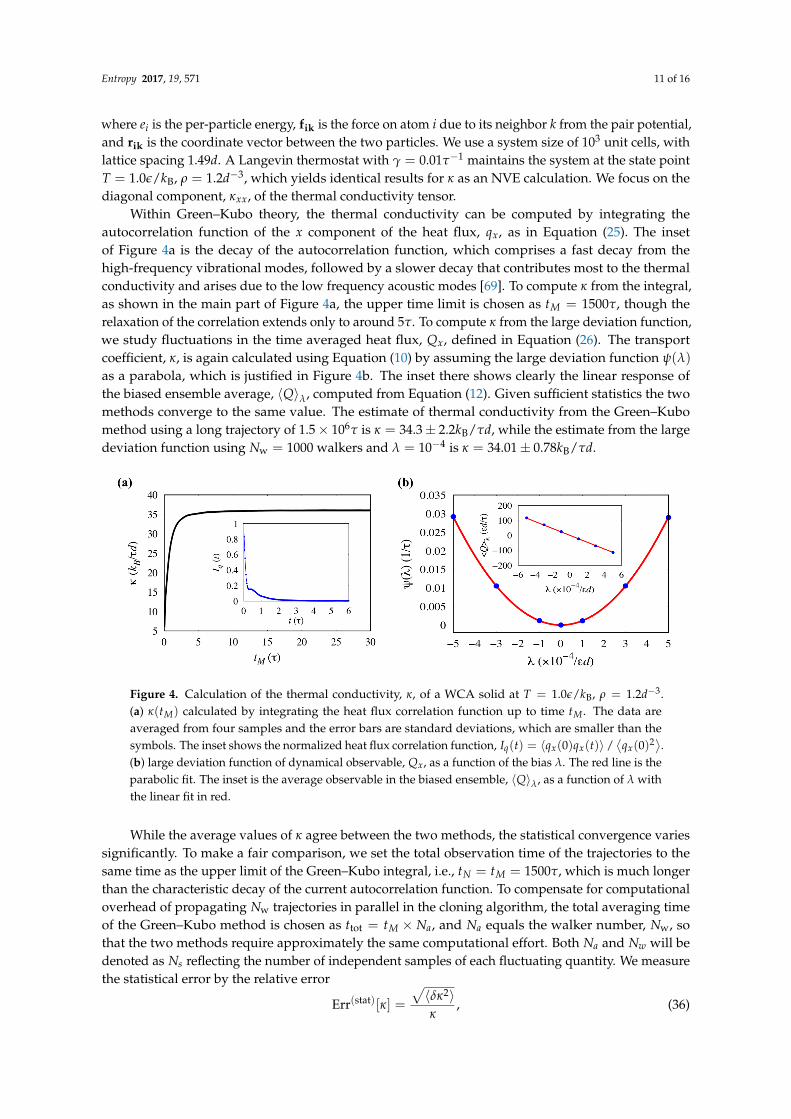
Within Green–Kubo theory, the thermal conductivity can be computed by integrating theautocorrelation function of the x component of the heat flux, qx, as in Equation (25). The insetof Figure 4a is the decay of the autocorrelation function, which comprises a fast decay from thehigh-frequency vibrational modes, followed by a slower decay that contributes most to the thermalconductivity and arises due to the low frequency acoustic modes [69]. To compute κ from the integral,as shown in the main part of Figure 4a, the upper time limit is chosen as tM = 1500τ, though therelaxation of the correlation extends only to around 5τ. To compute κ from the large deviation function,we study fluctuations in the time averaged heat flux, Qx, defined in Equation (26). The transportcoefficient, κ, is again calculated using Equation (10) by assuming the large deviation function ψ(λ)

as a parabola, which is justified in Figure 4b. The inset there shows clearly the linear response ofthe biased ensemble average, 〈Q〉λ, computed from Equation (12). Given sufficient statistics the twomethods converge to the same value. The estimate of thermal conductivity from the Green–Kubomethod using a long trajectory of 1.5× 106τ is κ = 34.3± 2.2kB/τd, while the estimate from the largedeviation function using Nw = 1000 walkers and λ = 10−4 is κ = 34.01± 0.78kB/τd.

Figure 4. Calculation of the thermal conductivity, κ, of a WCA solid at T = 1.0ε/kB, ρ = 1.2d−3.(a) κ(tM) calculated by integrating the heat flux correlation function up to time tM. The data areaveraged from four samples and the error bars are standard deviations, which are smaller than thesymbols. The inset shows the normalized heat flux correlation function, Iq(t) = 〈qx(0)qx(t)〉 /

⟨qx(0)2⟩.

(b) large deviation function of dynamical observable, Qx, as a function of the bias λ. The red line is theparabolic fit. The inset is the average observable in the biased ensemble, 〈Q〉λ, as a function of λ withthe linear fit in red.

While the average values of κ agree between the two methods, the statistical convergence variessignificantly. To make a fair comparison, we set the total observation time of the trajectories to thesame time as the upper limit of the Green–Kubo integral, i.e., tN = tM = 1500τ, which is much longerthan the characteristic decay of the current autocorrelation function. To compensate for computationaloverhead of propagating Nw trajectories in parallel in the cloning algorithm, the total averaging timeof the Green–Kubo method is chosen as ttot = tM × Na, and Na equals the walker number, Nw, sothat the two methods require approximately the same computational effort. Both Na and Nw will bedenoted as Ns reflecting the number of independent samples of each fluctuating quantity. We measurethe statistical error by the relative error

Err(stat)[κ] =

√〈δκ2〉κ

, (36)

Entropy 2017, 19, 571 12 of 16

which is plotted in Figure 5 for both methods. As usual, the statistical error depends on both therelative size of observable fluctuations, and the number of independent samples. We find that as thestandard deviations of both methods scale as 1/

√Ns as expected, our importance sampling clearly

helps to suppress the statistical error compared to the Green–Kubo method with similar computationaleffort, decreasing the magnitude of the error by an order of magnitude at fixed Ns. Even though wehave to choose a bias small enough to guarantee a linear response, we do see that larger bias helps toyield statistically reliable results.

0.01

0.1

1

100 1000

Err

(sta

t)[κ

]

Ns

Green−Kubo

λ = 10−4

λ = 5×10−4

Figure 5. Relative statistical error in the measurement of κ, the Green–Kubo method (black) and thelarge deviation function method with λ = 10−4 (red) and λ = 5× 10−4 (blue). Ns denotes the numberof walkers Nw used in evaluating the large deviation function, or Na, an indicator of the total averagingtime in the Green–Kubo method. The solid lines are fits of function y = a/

√Ns.

Jones and Mandadapu have performed a rigorous error analysis on the estimates of Green–Kubotransport coefficients with the assumption that the current fluctuations follow a Gaussian process [6].They found that the variance of κ is a monotonically increasing function of tM, and arrived at an upperbound for the relative error

Err(stat)[κ] < 2√

tMttot

= 2

√1

Na, (37)

which depends only on the number of trajectory segments of length tM. As a consequence, the statisticsbecome worse when the system has longer correlation times, and there are no ways of controlling theintrinsic variance of the observable. On the other hand, in the large deviation method, the relativeerror in the large deviation function is

Err(stat)[ψ(λ)] =1

ψ(λ)

√ψ′′(λ)

Nw=

1λ2

√2

LNw|λ| > 0, (38)

which depends not only on the number of samples, in this case Nw, but also has a dependence on λ

and L. In general, as λ increases, the walkers will become more correlated. However, within the regimeof linear response, or to first order in λ, the number of uncorrelated walkers should be Nw. Because thelarge deviation function, ψ(λ), scales as λ2 while its second derivative, ψ

′′(λ), has no dependence on

λ, the relative size of the fluctuations can be tuned by changing λ away from 0. This is verified inFigure 5, where increased λ generates an order of magnitude reduction in the statistical error relativeto the Green–Kubo calculation. This decrease in the statistical error is also confirmed for a series of λs.This tunability afforded by the large deviation function calculation is the same advantage affordedby direct simulation of transport processes where the relative size of fluctuations is determined bythe size of the average current produced by driving the system away from equilibrium. Instead ofevaluating κ from the large deviation function directly, we could have derived it from the change in

Entropy 2017, 19, 571 13 of 16

the average current produced at a given λ. However, in such a case, the relative error would only scaleas |λ| rather than λ2.

4. Conclusions

In this paper, we have explored the possibility of calculating transport coefficients from a largedeviation function or a path ensemble free energy. The robustness of our method is tested by a varietyof model systems ranging in composition and complexity of molecular interactions. Our methodis general, and we expect the addition of importance sampling to be beneficial in instances wherestatistical errors are dominant. More precisely, our analysis shows that the systematic errors for boththe Green–Kubo calculation and the large deviation calculation are asymptotically the same if thetime correlation function decays faster than 1/t2. If the correlation function decays slower, thanthere will be a larger systematic error for the large deviation function calculation that will need tobe converged at large tN . In such cases, the form of this error follows from Equation 32 and scalesas 1/tN ln tN . Such slow decay is expected for low-dimensional systems where the current includeshydrodynamic modes. Our analysis of the relative statistical errors between the Green–Kubo and thelarge deviation function calculations show that our method requires generically fewer statisticallyuncorrelated samples for comparable statistical accuracy. This is a consequence of the importancesampling employed. The magnitude of this statistical efficiency, defined as Nw/Na, or the numberof independent samples needed for a given error, increases linearly with the size of the transportcoefficient, L, and increases rapidly with the increasing bias, as λ4.

While we have considered only linear response coefficients, our method can be easily extended tothe nonlinear regime or to off-diagonal entries in the Onsager matrix, where Green–Kubo formulas areeven more cumbersome to evaluate and few direct methods exist or can be formulated. These extensionsare possible since the diffusion Monte Carlo algorithm is capable of sampling rare fluctuations inthe non-Gaussian tails of the distribution. Moreover, it is also possible to probe the response aroundnonequilibrium steady states, as the method presented here does not rely on an underlying Boltzmanndistribution.

Acknowledgments: D.T.L. and C.Y.G. was supported by the UC Berkeley College of Chemistry. The authorswould like to thank Ushnish Ray for useful discussions and for developing the use of LAMMPS with the CANSSpackage, available at https://github.com/ushnishray/CANSS for the calculation of nonequilibrium properties ofcomplex systems.

Author Contributions: C.Y.G. and D.T.L. conceived and designed the simulations; C.Y.G. performed thesimulations; C.Y.G. and D.T.L. analyzed the data; and C.Y.G. and D.T.L. wrote the paper.

Conflicts of Interest: The authors declare no conflict of interest.

References

1. Green, M.S. Markoff random processes and the statistical mechanics of time-dependent phenomena. II.Irreversible processes in fluids. J. Chem. Phys. 1954, 22, 398–413.

2. Kubo, R. Statistical-mechanical theory of irreversible processes. I. General theory and simple applications tomagnetic and conduction problems. J. Phys. Soc. Jpn. 1957, 12, 570–586.

3. Levesque, D.; Verlet, L.; Kürkijarvi, J. Computer “experiments” on classical fluids. IV. Transport propertiesand time-correlation functions of the Lennard–Jones liquid near its triple point. Phys. Rev. A 1973, 7, 1690.

4. Schelling, P.K.; Phillpot, S.R.; Keblinski, P. Comparison of atomic-level simulation methods for computingthermal conductivity. Phys. Rev. B 2002, 65, 144306.

5. Galamba, N.; de Nieto Castro, C.A.; Ely, J.F. Thermal conductivity of molten alkali halides from equilibriummolecular dynamics simulations. J. Chem. Phys. 2004, 120, 8676–8682.

6. Jones, R.E.; Mandadapu, K.K. Adaptive Green–Kubo estimates of transport coefficients from moleculardynamics based on robust error analysis. J. Chem. Phys. 2012, 136, 154102.

7. Evans, D.J.; Streett, W.B. Transport properties of homonuclear diatomics: II. Dense fluids. Mol. Phys. 1978,36, 161–176.

Entropy 2017, 19, 571 14 of 16

8. Hess, B. Determining the shear viscosity of model liquids from molecular dynamics simulations. J. Chem. Phys.2002, 116, 209–217.

9. Tenenbaum, A.; Ciccotti, G.; Gallico, R. Stationary nonequilibrium states by molecular dynamics. Fourier’slaw. Phys. Rev. A 1982, 25, 2778.

10. Baranyai, A.; Cummings, P.T. Steady state simulation of planar elongation flow by nonequilibrium moleculardynamics. J. Chem. Phys. 1999, 110, 42–45.

11. Hoover, W.G.; Evans, D.J.; Hickman, R.B.; Ladd, A.J.C.; Ashurst, W.T.; Moran, B. Lennard–Jones triple-pointbulk and shear viscosities. Green–Kubo theory, Hamiltonian mechanics, and nonequilibrium moleculardynamics. Phys. Rev. A 1980, 22, 1690.

12. Evans, D.J. Homogeneous NEMD algorithm for thermal conductivity—Application of non-canonical linearresponse theory. Phys. Lett. A 1982, 91, 457–460.

13. Mandadapu, K.K.; Jones, R.E.; Papadopoulos, P. A homogeneous nonequilibrium molecular dynamicsmethod for calculating thermal conductivity with a three-body potential. J. Chem. Phys. 2009, 130, 204106.

14. Müller-Plathe, F. A simple nonequilibrium molecular dynamics method for calculating the thermalconductivity. J. Chem. Phys. 1997, 106, 6082–6085.

15. Zhou, X.W.; Aubry, S.; Jones, R.E.; Greenstein, A.; Schelling, P.K. Towards more accurate molecular dynamicscalculation of thermal conductivity: Case study of GaN bulk crystals. Phys. Rev. B 2009, 79, 115201.

16. Tuckerman, M.E.; Mundy, C.J.; Balasubramanian, S.; Klein, M.L. Modified nonequilibrium moleculardynamics for fluid flows with energy conservation. J. Chem. Phys. 1997, 106, 5615–5621.

17. Tenney, C.M.; Maginn, E.J. Limitations and recommendations for the calculation of shear viscosity usingreverse nonequilibrium molecular dynamics. J. Chem. Phys. 2010, 132, 014103.

18. Geissler, P.L.; Dellago, C. Equilibrium time correlation functions from irreversible transformations intrajectory space. J. Phys. Chem. B 2004, 108, 6667–6672.

19. Touchette, H. The large deviation approach to statistical mechanics. Phys. Rep. 2009, 478, 1–69.20. Touchette, H. Introduction to dynamical large deviations of Markov processes. arXiv 2017, arXiv:1705.06492.21. Jarzynski, C. Nonequilibrium equality for free energy differences. Phys. Rev. Lett. 1997, 78, 2690.22. Crooks, G.E. Entropy production fluctuation theorem and the nonequilibrium work relation for free energy

differences. Phys. Rev. E 1999, 60, 2721–2726.23. Barato, A.C.; Seifert, U. Thermodynamic uncertainty relation for biomolecular processes. Phys. Rev. Lett.

2015, 114, 158101.24. Gingrich, T.R.; Horowitz, J.M.; Perunov, N.; England, J.L. Dissipation bounds all steady-state current

fluctuations. Phys. Rev. Lett. 2016, 116, 120601.25. Gaspard, P. Multivariate fluctuation relations for currents. New J. Phys. 2013, 15, 115014.26. Andrieux, D.; Gaspard, P. Fluctuation theorem and Onsager reciprocity relations. J. Chem. Phys. 2004, 121,

6167–6174.27. Andrieux, D.; Gaspard, P. A fluctuation theorem for currents and non-linear response coefficients. J. Stat.

Mech. Theory Exp. 2007, doi:10.1088/1742-5468/2007/02/P02006.28. Dellago, C.; Bolhuis, P.G.; Csajka, F.S.; Chandler, D. Transition path sampling and the calculation of rate

constants. J. Chem. Phys. 1998, 108, 1964–1977.29. Geissler, P.L.; Dellago, C.; Chandler, D. Kinetic pathways of ion pair dissociation in water. J. Phys. Chem. B

1999, 103, 3706–3710.30. Geissler, P.L.; Dellago, C.; Chandler, D.; Hutter, J.; Parrinello, M. Autoionization in liquid water. Science

2001, 291, 2121–2124.31. Bolhuis, P.G.; Chandler, D.; Dellago, C.; Geissler, P.L. Transition path sampling: Throwing ropes over rough

mountain passes, in the dark. Annu. Rev. Phys. Chem. 2002, 53, 291–318.32. Radhakrishnan, R.; Schlick, T. Orchestration of cooperative events in DNA synthesis and repair mechanism

unraveled by transition path sampling of DNA polymerase β’s closing. Proc. Natl. Acad. Sci. USA 2004,101, 5970–5975.

33. Basner, J.E.; Schwartz, S.D. How enzyme dynamics helps catalyze a reaction in atomic detail: A transitionpath sampling study. J. Am. Chem. Soc. 2005, 127, 13822–13831.

34. Hagan, M.F.; Chandler, D. Dynamic pathways for viral capsid assembly. Biophys. J. 2006, 91, 42–54.35. Peters, B. Recent advances in transition path sampling: Accurate reaction coordinates, likelihood maximisation

and diffusive barrier-crossing dynamics. Mol. Simul. 2010, 36, 1265–1281.

Entropy 2017, 19, 571 15 of 16

36. Limmer, D.T.; Chandler, D. Theory of amorphous ices. Proc. Natl. Acad. Sci. USA 2014, 111, 9413–9418.37. Giardina, C.; Kurchan, J.; Peliti, L. Direct evaluation of large-deviation functions. Phys. Rev. Lett. 2006,

96, 120603.38. Giardina, C.; Kurchan, J.; Lecomte, V.; Tailleur, J. Simulating rare events in dynamical processes. J. Stat. Phys.

2011, 145, 787–811.39. Nemoto, T.; Bouchet, F.; Jack, R.L.; Lecomte, V. Population-dynamics method with a multicanonical feedback

control. Phys. Rev. E 2016, 93, 062123.40. Klymko, K.; Geissler, P.L.; Garrahan, J.P.; Whitelam, S. Rare behavior of growth processes via umbrella

sampling of trajectories. arXiv 2017, arXiv:1707.00767.41. Ray, U.; Chan, G.K.-L.; Limmer, D.T. Exact fluctuations of nonequilibrium steady states from approximate

auxiliary dynamics. arXiv 2017, arXiv:1708.09482.42. Onsager, L. Reciprocal relations in irreversible processes. I. Phys. Rev. 1931, 37, 405.43. Palmer, T.; Speck, T. Thermodynamic formalism for transport coefficients with an application to the shear

modulus and shear viscosity. J. Chem. Phys. 2017, 146, 124130.44. Abascal, J.L.F.; Vega, C. A general purpose model for the condensed phases of water: TIP4P/2005. J. Chem. Phys.

2005, 123, 234505.45. Weeks, J.D.; Chandler, D.; Andersen, H.C. Role of repulsive forces in determining the equilibrium structure

of simple liquids. J. Chem. Phys. 1971, 54, 5237–5247.46. Chandler, D. Introduction to Modern Statistical Mechanics; Oxford University Press: London, UK, 1987.47. Morriss, G.P.; Evans, D.J. Statistical Mechanics of Nonequilbrium Liquids; ANU Press: Canberra, Australia, 2013.48. Lebowitz, J.L.; Spohn, H. A Gallavotti–Cohen-type symmetry in the large deviation functional for stochastic

dynamics. J. Stat. Phys. 1999, 95, 333–365.49. Helfand, E. Transport coefficients from dissipation in a canonical ensemble. Phys. Rev. 1960, 119, 1.50. Foulkes, W.M.C.; Mitas, L.; Needs, R.J.; Rajagopal, G. Quantum Monte Carlo simulations of solids.

Rev. Mod. Phys. 2001, 73, 33.51. Hurtado, P.I.; Garrido, P.L. Spontaneous symmetry breaking at the fluctuating level. Phys. Rev. Lett. 2011,

107, 180601.52. Garrahan, J.P.; Jack, R.L.; Lecomte, V.; Pitard, E.; van Duijvendijk, K.; van Wijland, F. First-order dynamical

phase transition in models of glasses: An approach based on ensembles of histories. J. Phys. A Math. Theor.2009, 42, 075007.

53. Bodineau, T.; Lecomte, V.; Toninelli, C. Finite size scaling of the dynamical free-energy in a kineticallyconstrained model. J. Stat. Phys. 2012, 147, 1–17.

54. Allen, R.J.; Valeriani, C.; ten Wolde, P.R. Forward flux sampling for rare event simulations. J. Phys. Condens.Matter 2009, 21, 463102.

55. Frenkel, D.; Smit, B. Understanding Molecular Simulation: From Algorithms to Applications; Academic Press:San Diego, CA, USA, 2001; Volume 1.

56. Nemoto, T.; Hidalgo, E.G.; Lecomte, V. Finite-time and finite-size scalings in the evaluation of large-deviationfunctions: Numerical approach in continuous time. Phys. Rev. E 2017, 95, 062134.

57. Plimpton, S. Fast parallel algorithms for short-range molecular dynamics. J. Comput. Phys. 1995, 117, 1–19.58. Ray, U.; Chan, G.K.-L.; Limmer, D.T. Importance sampling large deviations in nonequilibrium steady states:

Part 1. arXiv 2017, arXiv:1708.00459.59. González, M.A.; Abascal, J.L.F. The shear viscosity of rigid water models. J. Chem. Phys. 2010, 132, 096101.60. Nosé, S. A unified formulation of the constant temperature molecular dynamics methods. J. Chem. Phys.

1984, 81, 511–519.61. Ryckaert, J.P.; Ciccotti, G.; Berendsen, H.J.C. Numerical integration of the cartesian equations of motion of a

system with constraints: Molecular dynamics of n-alkanes. J. Comput. Phys. 1977, 23, 327–341.62. Sendner, C.; Horinek, D.; Bocquet, L.; Netz, R.R. Interfacial water at hydrophobic and hydrophilic surfaces:

Slip, viscosity, and diffusion. Langmuir 2009, 25, 10768–10781.63. Petravic, J.; Harrowell, P. On the equilibrium calculation of the friction coefficient for liquid slip against a

wall. J. Chem. Phys. 2007, 127, doi:10.1063/1.2799186.64. Huang, K.; Szlufarska, I. Green–Kubo relation for friction at liquid–solid interfaces. Phys. Rev. E 2014,

89, 032119.

Entropy 2017, 19, 571 16 of 16

65. Bocquet, L.; Barrat, J.L. On the Green–Kubo relationship for the liquid–solid friction coefficient. J. Chem. Phys.2013, 139, 044704.

66. Alder, B.J.; Wainwright, T.E. Decay of the velocity autocorrelation function. Phys. Rev. A 1970, 1, 18–21.67. Wainwright, T.; Alder, B.; Gass, D. Decay of time correlations in two dimensions. Phys. Rev. A 1971, 4, 233.68. Isobe, M. Long-time tail of the velocity autocorrelation function in a two-dimensional moderately dense

hard-disk fluid. Phys. Rev. E 2008, 77, 021201.69. Che, J.; Cagin, T.; Goddard, W.A., III. Thermal conductivity of carbon nanotubes. Nanotechnology 2000,

11, 65–69.

c© 2017 by the authors. Licensee MDPI, Basel, Switzerland. This article is an open accessarticle distributed under the terms and conditions of the Creative Commons Attribution(CC BY) license (http://creativecommons.org/licenses/by/4.0/).