Embed Size (px)
Citation preview
Transmissionslösningar för stora havsbaserade vindkraftsparkerTransmission alternatives for grid connection of large offshore wind farms
Désirée Moberg
EN1302Examensarbete för civilingenjörsexamen i energiteknik, 30 hp)
Report Number U 13:07 Désirée Moberg, Umeå University 2012-02-08
THESIS WORK TRANSMISSION ALTERNATIVES FOR GRID CONNECTION OF LARGE OFFSHORE WIND FARMS AT LARGE DISTANCE
VATTENFALL RESEARCH & DEVELOPMENT AB BA R&D - Wind & Ocean power

TRANSMISSION ALTERNATIVES FOR GRID CONNECTION OF LARGE OFFSHORE WIND FARMS AT LARGE DISTANCE
From Date Serial No.
Vattenfall Research and Development AB 2013-02-08 U 13:07
Author/s Security class Project No.
Désirée Moberg Internal [S2] PR.270.3.14.2
Customer Reviewed by
Urban Axelsson
Issuing authorized by
Viktoria Niemane
Sven-Erik Thor
Key Word No. of pages Appending pages
Transmission network, offshore wind, HVAC, HVDC, EeFarm II
43 12

Distribution list
Company Department Name Number of

Summary
With the great possibility of offshore wind power that can be installed in the world seas, offshore wind power is starting to get and important source of energy. The growing sizes of wind turbines and a growing distance to land, makes the choice of transmission alternative to a more important factor. The profitability of the transmission solution is affected by many parameters, like investment cost and power losses, but also by parameters like operation & maintenance and lead time of the system.
The study is based on a planned wind farm with a rated power of 1 200 MW and at a distance of 125 km to the connection point. Four models have been made for the transmission network with the technology of HVAC, HVDC and a hybrid of both. The simulation program used is EeFarm II, which has an interface in Matlab and Simulink. The four solutions have been compared technically, with difficulties and advantages pointed out and also economically, with the help of LCOE, NPV and IRR. Costs, power losses and availability of the wind turbines and intra array network are not included in the study.
The result of the simulations implies that the HVAC solution is the most profitable with the lowest Levelized Cost of Energy and highest Net Price Value and Internal Rate of Return. The values are 25.11 €/MWh, 387.60 M€ and 15.32 % respectively. A HVDC model with just one offshore converter station, has a LCOE close to the HVAC solution, but with a more noticeable difference in NPV and IRR (25.71 €/MWh, 300.76 M€ and 14.84 % respectively).
A sensitivity analysis has been done, where seven different parameters have been changed for analysing their impact on the economic result. The largest impact made was by a change in investment cost and lead times. The results imply that with a structure of the transmission network as for the models, and with similar input data, the break point where a HVDC solution is more profitable than a HVAC solution is not yet passed at a distance of 125 km from the connection point. With an evolving technology in the field of HVDC, a shorter lead time and lower investment cost could mean that a HVDC solution would be more profitable at this distance. Difficulties for a HVAC solution with more cable required, like bigger land usage and cable manufacturing as a bottle neck, could make an important factor tough while making a decision.
Sammanfattning
Med den stora potentialen hos världens hav, börjar havsbaserad vindkraft bli en betydande energikälla. Den ökande storleken på vindkraftsturbinerna tillsammans med de ökade avstånden mellan vindkraftsparkerna och land, gör att transmissionslösningen blir en mer betydelsefull komponent. Flera olika parametrar kan vara avgörande för transmissionslösningens lönsamhet, som investeringskostnad och effektförluster, men också saker som drift & underhåll och projektets ledtid.
Studien är baserad på en planerad vindkraftspark med en märkeffekt på 1 200 MW och på ett avstånd på 125 km till anslutningspunkten. Fyra modeller av transmissionssnätet har gjorts, där tekniken har bestått av HVAC, HVDC samt en blandning av dessa. Simuleringarna har gjort i EeFarm II, ett program baserat på Matlab och Simulink. De fyra modellerna har jämförts tekniskt, med för- och nackdelar poängterade, och även ekonomiskt med hjälp av LCOE, NPV och IRR. Kostnader, effektförluster och tillgängligheten för vindkraftsturbinerna och internnätet i vindkraftsparken är inte inkluderade i studien.
Resultaten av simuleringarna visar på att HVAC-lösningen är den mest lönsamma, med lägst Levelized Cost of Energy och högst Net Price Value och Internal Rate of Return. Värdena för dessa är 25,11 €/MWh, 387,60 M€ respektive 15,32 %. En HVDC-lösning med enbart en DC-plattform och likriktarstation för hela märkeffekten, har en LCOE inte långt ifrån HVAC-lösningen, men med en lite större skillnad i NPV och IRR (25,71 €/MWh, 300,76 M€ respektive 14,84 %).
För att analysera påverkan av olika parametrar på de ekonomiska mätvärdena, har en osäkerhetsanalys gjort. Den största påverkan på resultatet syntes av förändringar av investeringskostnader och ledtider. Ovanstående resultat tyder på, med transmissionslösningar enligt modellerna i detta arbete, att brytpunkten där en HVDC-lösning är mer lönsam än en HVAC-lösning inte än är passerad vid ett avstånd på 125 km till anslutningspunkten. Med en fortfarande väldigt ung teknik för HVDC, kan den ständigt utvecklande tekniken i framtiden betyda kortare ledtider och en lägre investeringskostnad för en HVDC-lösning och möjligheten att vara en mer lönsam lösning. Komplikationer med en HVAC-lösning pga den extra landkabeln, som större landanvändning och med kabeltillverkningen som en flaskhals, kan ändå göra en HVDC-lösning mer praktisk.
Table of Content Page
1 LIST OF ACRONYMS AND ABBREVIATIONS 1
2 INTRODUCTION 1
2.1 Background 1 2.2 Purpose 3 2.3 Goal 3
3 ECONOMICS OF OFFSHORE WIND POWER 3
3.1 Financing wind power 3 3.1.1 Market regulations 3 3.1.2 Risks with offshore wind 5 3.1.3 Investing in offshore wind 6
3.2 Economic metrics 6 3.2.1 Levelized Cost of Energy 6 3.2.2 Net Present Value 8 3.2.3 Internal Rate of Return 8 3.2.4 Advantages and disadvantages with the metrics 8
3.3 Availability 10 3.4 Capacity factor 11 3.5 Sensitivity analysis 11
4 THE TECHNOLOGY 12
4.1 Export cables 12 4.1.1 HVAC cables 12 4.1.2 HVDC cables 13
4.2 Sea laying 13 4.3 Transformers 14 4.4 Reactive compensation 14 4.5 Challenges of the transmission network 15
5 SIMULATIONS OF TRANSMISSION ALTERNATIVES 16
5.1 About EeFarm II 16 5.2 Background for modeling 18 5.3 HVAC model 19 5.4 HVDC models 21
5.4.1 2x600 MW HVDC solution 21 5.4.2 1x1200 MW HVDC solution 23

5.5 Hybrid model 24 5.6 Economic models 26
5.6.1 Economic parameters 26 5.6.2 Lead time 26 5.6.3 Pay plan 27
6 RESULT 27
6.1 HVAC model 28 6.2 HVDC models 29
6.2.1 2x600 MW HVDC solution 29 6.2.2 1x1200 MW HVDC solution 31
6.3 Hybrid model 32 6.4 Sensitivity analysis 34
6.4.1 Investment cost 34 6.4.2 O&M cost 35 6.4.3 Lifetime 35 6.4.4 Unavailability 36 6.4.5 Capacity factor 36 6.4.6 Distance to connection point 37 6.4.7 Redundancy 38 6.4.8 Lead time 38
7 DISCUSSION 39
8 CONCLUSIONS 40
9 ACKNOWLEDGEMENTS 40
10 REFERENCES 41
10.1 Pictures 43
Appendices Number of Pages
APPENDIX A HVAC EeFarm II model, 3 x 400 MW 2
APPENDIX B HVDC EeFarm II model 1, 2 x 600 MW 2
APPENDIX C HVDC EeFarm II model 2, 1 x 1 200 MW 1
APPENDIX D Hybrid EeFarm II model, 400 MW HVAC + 800 MW HVDC 1
APPENDIX E Pay plan 1
APPENDIX F Investment costs 3
APPENDIX G O&M cost 1
APPENDIX H Availability 1
Vattenfall Research and Development AB U 12:xx (Internal [S2])
Page 1 (43)
1 List of acronyms and abbreviations
AUE Annual Utilized Energy
CF Capacity Factor
CRF Capital Recovery Factor
EAONE East Anglia ONE
EAOW East Anglia Offshore Wind
ENS Energy Not Supplied
HVAC High Voltage Alternating Current
HVDC High Voltage Direct Current
IRR Internal Rate of Return
LEC Levy Exemption Certificates
LCOE Levelised Cost Of Energy
NPV Net Present Value
O&M Operation and Maintenance
OFTO Offshore Transmission Owner
ROC Renewable Obligation Certificate
TSO Transmission System Operator
2 Introduction
2.1 Background
Without CO2-emissions and other greenhouse gases, no hazardous waste left behind, wind power is a very good alternative for producing energy. Unlike coal and nuclear plants, it doesn’t swallow huge amounts of water either, which is starting to become a scarce resource. The seas have great possibilies for offshore wind farms and by putting the wind turbines offshore, people get less affected and don’t have to see them. But putting them onshore is today a more economical solution. Offshore wind farms take longer time to develop depending on its more hostile environment, having more expensive technology and is harder to reach for operation and maintenance. The prices will probably be decreased though, as offshore turbines starts to manufactures on a larger scale and make it a more competitive energy resource. [1] The first offshore wind farm was commissioned 1991, 2,5 km off the Danish coast at Vindeby and consists of eleven 450 kW turbines. 19 years later 1 132 offshore turbines existed across Europe [2]. In fact, EU is word leading in offshore wind power with 4 000 MW installed power. Just being in the beginning of a major industrial development, EWEA estimates that 40 GW of offshore wind will be istalled by 2020. That would annually produce 148 TWh, meeting over 4% of the EUs total electricity demand and avoiding 87 million tonnes of CO2 emissions [3].
Getting a perspective on the magnitude of wind turbines, both the size and power generation, can be a bit hard. During a conference, Offshore Wind
Economics and Finance 2012, a man from Typhoon Offshore compared the blades of the wind turbine to London Eye and its tower the Statue of Liberty, which gives a

Vattenfall Research and Development AB U 12:xx (Internal [S2])
Page 2 (43)
pretty rough estimation of how big a wind turbine is. London Eye has a diameter of 120 m [4], which can be compared to a diameter of 154 m for Siemens 6-MW wind turbine or 164 m for Vestas 8 MW turbine. The height of the tower depends of the site, but can be as much as 135 m [5] while the Statue of Liberty has a height of 93 m from ground to torch [6]. Now having a perspective on how big it is, how much do we expect it to generate? Assume the capacity factor, i.e. the power generated by a farm divided by the maximum power it would be able to deliver at a certain site, to be 0.4. That would give us an electricity generation of a 21 GWh for a Siemens 6 MW turbine and 28 GWh for a Vestas 8 MW turbine. The electric power consumption in Sweden is about 15 MWh per capita [7], which means that one wind turbine could support around 1 400 to 1 800 people in Sweden with renewable electricity.
Offshore wind power is starting to be an important energy source for renewables. As the technology of wind power evolves and wind turbines gets bigger and bigger, so does also the sizes of offshore wind farms together with their distance to land. With a great amount of electricity to transmit to the electric grid, the transmission solution is of big impact. The efficiency of the solution depends of many things, like investment cost, power losses and lead times just to mention a few.
A lot of wind capacity is planned to be installed offshore, with Vattenfall involved in many of the projects. A license to develop approximately 7 200 MW wind capacity outside the east coast of England has been assigned to EAOW, East Anglia Offshore Wind Limited, a Joint Venture company between Scottish Power Renewables and Vattenfall Wind Power Limited. The technical and economical assumptions in this study are based on the first of 6 zones, all with 1 200 MW capacity, which has been modeled for comparing transmission by HVAC and HVDC. This zone, EAONE (East Anglia ONE) has a distance to shoreline of 90 km and then 35 km more before reaching the connection point at Bramford, measured from the collection platforms located in the wind farm. With focus on the transmission network, this model will take no concerns to costs and failure for the turbines and intra array network.
As the wind turbines started to be placed offshore, the same technology was used as for onshore wind farms. AC-technology is a far more developed technology and is not as expensive as the HVDC technology for short distances to land. A HVAC solution requires more cables than a corresponding HVDC solution, which implies higher cost due to cable laying, but also bigger electric losses in the cables. That makes a HVDC solution a more economic alternative at a long distance to land.
Vattenfall Research and Development AB U 12:xx (Internal [S2])
Page 3 (43)
2.2 Purpose
An economical/technical comparison of different transmission alternatives is made in the simulation program EeFarm II for Vattenfall Research & Development AB. A comparison is of interest both for the grand project EAONE, but also for upcoming projects.
2.3 Goal
The studies of different transmission solutions was made by the simulation software EeFarm II, based on Matlab and Simulink. The goal was to create a HVAC model similar to a feasibility study of a third of the whole transmission made in the electric transmission program PSS/E, an HVDC model based on an ongoing feasibility study made in PSS/E with an HVDC model of half of the transmission, a model of an optimized solution by the developers and a model with mixed technology. The models will be compared both technically with the result from EeFarm II and economically with calculations made in Excel. As a fairly new technology, there are many uncertainties regarding both economical and technical variables, for which reason a sensitivity analysis is made. Impacts being evaluated are the investment cost, O&M cost, availability, capacity of the farm, distance to the connection point, lifetime and lead time of the farm.
3 Economics of offshore wind power
3.1 Financing wind power
3.1.1 Market regulations
For an unregulated market, there would be nothing to ensure that production occurs in socially and environmentally acceptable ways. Regulations are therefore needed for adding the external effects, not included in the price, like greenhouse gas emission, air pollution or environmental benefits from renewable energy sources. In general, there are two ways to control the market – either by price or quantity regulations. That means that the energy supplier can be paid an above-market price for the energy, while the market determines the quantity or be guaranteed a share of the energy supply while the market determines the energy price.
3.1.1.1 Price-driven regulations
Financial support is often given to suppliers of renewable energy, usually as a subsidy per kW of installed capacity or a payment per kWh produced and sold. A fixed regulated feed-in tariff (FIT) or a fixed premium is supplied from a governmental

Vattenfall Research and Development AB U 12:xx (Internal [S2])
Page 4 (43)
institution, utility or supplier, who is obligated to pay for renewable electricity. With FITs, the grid owner is ordered to buy renewable electricity at a politically determined price. This system is popular by wind developers since it secures a long term certainty of the sales price [8]. The alternative is a fixed premium to be added on the electricity price. In Europe, these premiums are financed by a levy on the energy bill of all electric consumers.
3.1.1.2 Quantity-driven regulations
Another way to make the market of renewables stronger is by quantity-driven regulations, where the government requires an increasing amount of the electricity supply to be based on renewable energy sources. This can be done either by a tradable certificate system or by a trading/ bidding system. With tradable certificate system, referring to green certificates or renewable portfolios, the wind developers are paid a variable premium above market price of electricity, where the price is determined according to the market for these certificates. It may lead to highly volatile prices due to political uncertainty surrounding the size or future renewable energy obligations [8]. A trading/ bidding system amplifies a specific amount of electricity or capacity is called for tender and result in contract winners receiving a guaranteed tariff for a certain period of time. A politically determined amount of renewable energy is here ordered for the electrical supply, where the cost is shared among electricity consumers.
3.1.1.3 Indirect strategies
Besides price- and quantity-driven mechanisms, where one specific renewable energy technology is being promoted, there are other strategies with an indirect promotion of renewables. Such strategies would be environmental taxes on energy for non-renewable sources, taxes/permits on CO2 emissions and removal of previous subsidies given to fossil and nuclear generation.
3.1.1.4 Market regulations in Europe
A big mixture of different market regulations are used in Europe. According to “Svensk Energi” (Swedish Energy), the most effective would be to use the same regulations, based on certificates in the whole EU [9]. Since the beginning of 2012, Sweden and Norway have had a shared system, neutral to type of renewable, leading up to that the most economical project will be realized. No separate system exists to the benefit of offshore wind power in Sweden, which makes the probability of building an offshore wind farm in Sweden low. In UK, support to wind power has been given in terms of ROCs (Renewable obligation certificates) where an amount of ROCs are paid per MWh of delivered electricity. The ROCs received for offshore wind is a bit higher than onshore wind because of the more expensive technology. On top of the price for base load, a Levy Exemption Certificate (LEC) is added to the energy bill, an evidence of Climate Change Levy that is exempted to energy supply

Vattenfall Research and Development AB U 12:xx (Internal [S2])
Page 5 (43)
generated from qualifying renewable sources. This certificate system will be changed though and can only be used by projects starting there operation before 2018. A new system, FIT CfD (Feed-in Tariff with Contract for Difference), will take over. With this system, the generator will receive a top payment if the wholesale electricity price is below the price agreed in the contract and for the opposite situation pay the surplus back. This long-term contract will stabilize the revenues and reduce the investment risk [10].
3.1.2 Risks with offshore wind
A large project such as an offshore wind farm comes with a lot of economical risks, but with knowledge and by taking them into account, they are possible to manage. The environment for these projects is very harsh and if things go wrong, they often go really wrong. With a big water depth, lost equipment is hard to get back, if even possible at all.
Different periods of the project have its own risks, like during the development of the project with it being relatively expensive and dependent on availability of finance. A multi contractual structure together with sensibility to planning delays also makes a risk. Different governments have different drivers in how to encourage renewables, where uncertainties are brought regarding long term economical support.
The location of the wind farm brings many construction risks, as loss of equipment and bad weather, which can interrupt work, make a danger for the people working there and lead to delays. Constrains in the supply chain also makes a risk with a shortage of wind turbines, vessels, pilling hammers, suitable harbors and a shortage in people with knowledge to construct these projects.
With a young and inexperienced market such as offshore wind power, the technology itself makes a big risk too. It is a fast developing market, where the developers have to make a stand between using the newest technology on the market or the older more experienced technology, which is followed by many projects being prototypes. The offshore turbines are normally larger than onshore and have to be suited for the tougher environment, which makes them more complex. The HVDC technology is preferable at long distances, by reasons that will be discussed later on, but is not as well known as the HVAC technology and therefore makes a risk.
During operation the wind is one of the key concerns for the economy of the project. The behavior of the wind offshore is not fully understood and makes an uncertainty in wind resource and energy yield. Once again the weather makes a big risk, with bringing danger to people and technology and long repair times in case of failure due to lack of a weather window allowing a vessel to go out to the farm. The cost of O&M is still not very certain either, even for HVAC [11].
Vattenfall Research and Development AB U 12:xx (Internal [S2])
Page 6 (43)
3.1.3 Investing in offshore wind
Between 2010 and 2020 the installed capacity of European offshore wind power is expected to grow from 3 GW to 40 GW [3], which is expected to require approximately 130 G€ of investments in Europe [12]. So how should this explosion of offshore wind power be financed and why should companies invest in it? The costs of offshore wind power are still high due to few players on the market. Offshore wind power has been identified as an attractive asset class by leading financial investors due to many reasons. It brings attractive and stable long term revenues with a long term exposure to energy prices and inflation and the correlation to return from other asset classes is low. Compared to other asset types, such as investment in real estate and infrastructure, there is a short pay-back time for the investment and gives a long term income stream [12]. Traditionally the equity for these projects is found in utilities, but that is not enough anymore and new investors are needed. For breaking down the cost, different parts of the project can have different investors, like one for the transmission network and one for the wind turbines, but ending up with a higher risk of delays due to more contracts. An electric utility is needed as a corner stone investor with its knowledge in the industry and the risks of the project. A reason for other companies to invest in wind power may be because of corporate social responsibility, CSR, a way for the company to reduce their CO2-footprint and for branding the company. With the electric utility having the knowledge it is not necessary for these companies to know anything about the technology of wind power. A third group of investors would be the financial investors, investing in it for the economical benefits [13].
3.2 Economic metrics
Comparison of two projects can be made in many ways, both by technology with advantages and losses and economically with revenues and profitability. For comparing the economics of two projects there are a set of metrics to calculate. A very common metric to use for comparing technology producing energy is Levelized Cost of Energy, LCOE, where the mean cost per unit of produced energy over the plants lifetime is calculated (€ /MWh). Other very common metrics are the Net Present Value, NPV, and Internal Rate of Return, IRR.
3.2.1 Levelized Cost of Energy
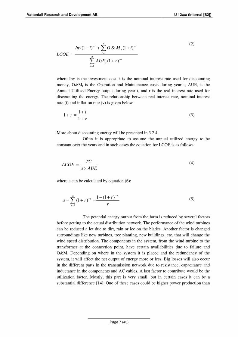
A very common metric for comparing projects regarding energy production is LCOE (Levelized cost of energy) or LPC (Levelised Production Cost) as it is referred to in EeFarm II, where the mean cost per unit of produced energy over the plants lifetime is calculated (€ /MWh). Both total costs and energy yield are discounted to the start of the project.
Vattenfall Research and Development AB U 12:xx (Internal [S2])
Page 7 (43)
(2)
where Inv is the investment cost, i is the nominal interest rate used for discounting money, O&Mt is the Operation and Maintenance costs during year t, AUEt is the Annual Utilized Energy output during year t, and r is the real interest rate used for discounting the energy. The relationship between real interest rate, nominal interest rate (i) and inflation rate (v) is given below
(3)
More about discounting energy will be presented in 3.2.4.
Often it is appropriate to assume the annual utilized energy to be constant over the years and in such cases the equation for LCOE is as follows:
(4) where a can be calculated by equation (6):
(5)
The potential energy output from the farm is reduced by several factors
before getting to the actual distribution network. The performance of the wind turbines can be reduced a lot due to dirt, rain or ice on the blades. Another factor is changed surroundings like new turbines, tree planting, new buildings, etc. that will change the wind speed distribution. The components in the system, from the wind turbine to the transformer at the connection point, have certain availabilities due to failure and O&M. Depending on where in the system it is placed and the redundancy of the system, it will affect the net output of energy more or less. Big losses will also occur in the different parts in the transmission network due to resistance, capacitance and inductance in the components and AC cables. A last factor to contribute would be the utilization factor. Mostly, this part is very small, but in certain cases it can be a substantial difference [14]. One of these cases could be higher power production than
∑
∑
=
−
−
=
−
+
+++
=n
t
t
t
tn
t
t
t
rAUE
iMOiInv
LCOE
1
1
)1(
)1(&)1(
v
ir
+
+=+
11
1
AUEa
TCLCOE
×
=
r
rra
nn
t
t−
=
−+−
=+=∑)1(1
)1(1
Vattenfall Research and Development AB U 12:xx (Internal [S2])
Page 8 (43)
load of the system during high wind and low load periods, which means that the excess energy has to be dissipated during these periods.
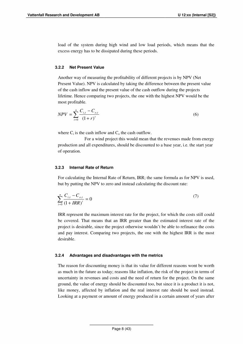
3.2.2 Net Present Value
Another way of measuring the profitability of different projects is by NPV (Net Present Value). NPV is calculated by taking the difference between the present value of the cash inflow and the present value of the cash outflow during the projects lifetime. Hence comparing two projects, the one with the highest NPV would be the most profitable.
(6) where Ci is the cash inflow and Co the cash outflow. For a wind project this would mean that the revenues made from energy production and all expenditures, should be discounted to a base year, i.e. the start year of operation.
3.2.3 Internal Rate of Return
For calculating the Internal Rate of Return, IRR; the same formula as for NPV is used, but by putting the NPV to zero and instead calculating the discount rate:
(7) IRR represent the maximum interest rate for the project, for which the costs still could be covered. That means that an IRR greater than the estimated interest rate of the project is desirable, since the project otherwise wouldn’t be able to refinance the costs and pay interest. Comparing two projects, the one with the highest IRR is the most desirable.
3.2.4 Advantages and disadvantages with the metrics
The reason for discounting money is that its value for different reasons wont be worth as much in the future as today; reasons like inflation, the risk of the project in terms of uncertainty in revenues and costs and the need of return for the project. On the same ground, the value of energy should be discounted too, but since it is a product it is not, like money, affected by inflation and the real interest rate should be used instead. Looking at a payment or amount of energy produced in a certain amount of years after
∑=
+
−
=
n
tt
toti
r
CCNPV
0
,,
)1(
∑=
=
+
−n
tt
toti
IRR
CC
0
,, 0)1(

Vattenfall Research and Development AB U 12:xx (Internal [S2])
Page 9 (43)
commission, the size of it would not be affected by how long the lead time is and how far in the future it is made. But as an example, the value today of a payment made in 10 years would be much less than if it was to be done in 5 years.
With payments distributed over the lead time, longer lead times would mean that the discounted costs will be lower compared to a likewise solution with a shorter lead time. A longer lead time would also mean that the discounted energy will be lower, but will be affected much more than the discounted investment cost, since just parts of the investment cost will be postponed in contrast to the amount of generated energy. With an energy production that is more affected by lead times than cost, longer lead times will negatively affect the LCOE, making it higher. The affection on investment cost and generated energy by lead time included in the model is visualized in Figure 1. The project has a lifetime of 10 years, payments divided in three equal parts, where the first one is paid directly.
With uncertainties in electric prices and market regulations to be used,
LCOE has an advantage of not taking the revenues into account. That means that projects without revenues or parts of a system generating revenues can be evaluated. The downside is that projects can be non profitable for a company without being noticeable on the LCOE. In that way a metric like NPV can be more suitable to use.
Figure 1: Effect on investment cost and generated energy by lead times included in the
model
Vattenfall Research and Development AB U 12:xx (Internal [S2])
Page 10 (43)
Comparing projects with the help of NPV has its positive and negative sides. Like LCOE, it takes in account for the time value of money and is a good way to compare two projects with the same lifetime. It is also a well known measurement and could therefore be easier for people to relate to. The NPV is very sensitive to the size of lifetime, wherefore two projects of different lifetime can not be compared. As for the calculation of LCOE the discount rate is approximated to be fixed, which is not entirely true, and could give a different result with its changes. NPV is measured in a chosen currency; euro, dollar or pounds for example, which can obstruct comparison between projects, but a bigger limitation is that it doesn’t compare the net value of gained money to the magnitude of the investment cost or time it took to achieve it.
One simplification made in the equations for LCOE is that the interest rate is uniform through the period, which is not really true. The choice of interest rate affects the estimation of net return from the project – a high interest rate will favor projects with low investment cost and higher O&M cost and in the opposite direction a low interest rate will favor projects with high investment costs and lower O&M costs [15]. An advantage of the IRR is that it doesn’t depend on an estimation of the interest rate, but can be a bit harder to relate to than NPV. IRR is calculated by iterations in these models and is by that more time demanding to calculate than the other metrics. If the amount of energy generated would be the same each year it would be possible to calculate it without iterations, but because of different time of commissioning for certain parts of the farm that is not the case. More about commissioning will be covered later on in the report.
3.3 Availability
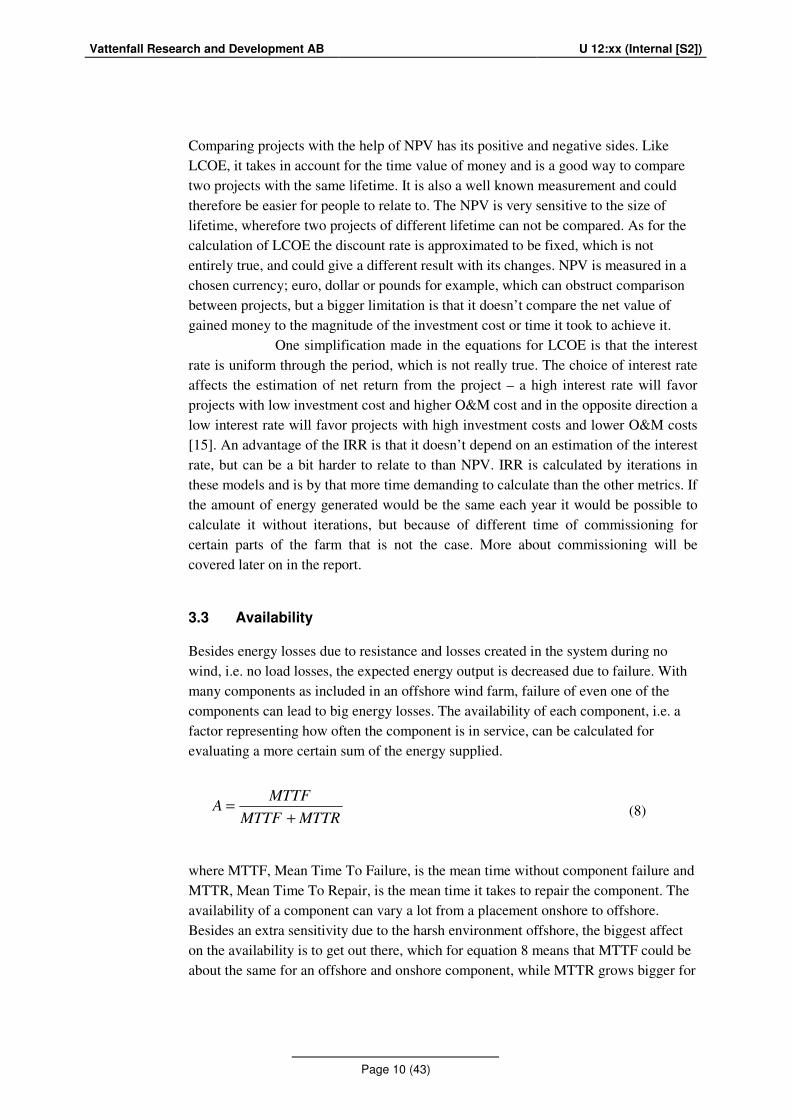
Besides energy losses due to resistance and losses created in the system during no wind, i.e. no load losses, the expected energy output is decreased due to failure. With many components as included in an offshore wind farm, failure of even one of the components can lead to big energy losses. The availability of each component, i.e. a factor representing how often the component is in service, can be calculated for evaluating a more certain sum of the energy supplied.
(8) where MTTF, Mean Time To Failure, is the mean time without component failure and MTTR, Mean Time To Repair, is the mean time it takes to repair the component. The availability of a component can vary a lot from a placement onshore to offshore. Besides an extra sensitivity due to the harsh environment offshore, the biggest affect on the availability is to get out there, which for equation 8 means that MTTF could be about the same for an offshore and onshore component, while MTTR grows bigger for
MTTRMTTF
MTTFA
+
=
Vattenfall Research and Development AB U 12:xx (Internal [S2])
Page 11 (43)
a component located offshore [16]. Examples of variables affecting the availability is method of transport, availability of transport, weather conditions, location of offshore platform, location of air field/port/offshore maintenance platform and availability of required personnel. The time it takes to repair a component can differ a lot – correct administration procedure for rapidly deploying required personnel together with traveling by a helicopter in good weather can lead to a repair time of only one day, while bad weather conditions and unavailability of a large suitable vessel can extend it to over three months [16]. Sometimes it can therefore be more economical to invest in a redundant system, with an extra parallel cable or an extra transformer, ready for deployment if its counterpart breaks.
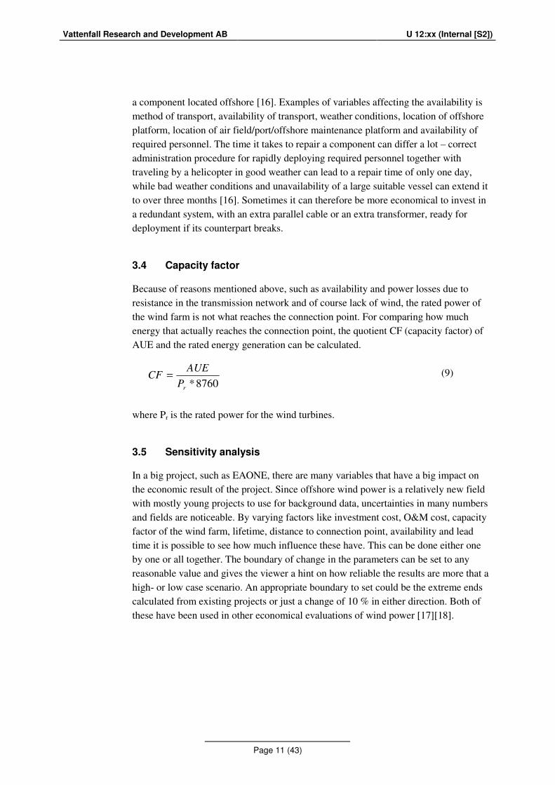
3.4 Capacity factor
Because of reasons mentioned above, such as availability and power losses due to resistance in the transmission network and of course lack of wind, the rated power of the wind farm is not what reaches the connection point. For comparing how much energy that actually reaches the connection point, the quotient CF (capacity factor) of AUE and the rated energy generation can be calculated.
(9) where Pr is the rated power for the wind turbines.
3.5 Sensitivity analysis
In a big project, such as EAONE, there are many variables that have a big impact on the economic result of the project. Since offshore wind power is a relatively new field with mostly young projects to use for background data, uncertainties in many numbers and fields are noticeable. By varying factors like investment cost, O&M cost, capacity factor of the wind farm, lifetime, distance to connection point, availability and lead time it is possible to see how much influence these have. This can be done either one by one or all together. The boundary of change in the parameters can be set to any reasonable value and gives the viewer a hint on how reliable the results are more that a high- or low case scenario. An appropriate boundary to set could be the extreme ends calculated from existing projects or just a change of 10 % in either direction. Both of these have been used in other economical evaluations of wind power [17][18].
8760*rP
AUECF =
Vattenfall Research and Development AB U 12:xx (Internal [S2])
Page 12 (43)
4 The technology
4.1 Export cables
4.1.1 HVAC cables
The choice of cable plays an important role in the transmission network. AC cables have a capacitive component which makes current flow into the cable to charge the cable capacitance and hence reduces the export current the cable can carry. There are also requirement on how much reactive effect that is ok to deliver at the connection point [19]. Besides by length, the capacitive contribution gets much larger at high voltages. With the help of reactors this problem can be controlled, but with the effect of increasing cost.
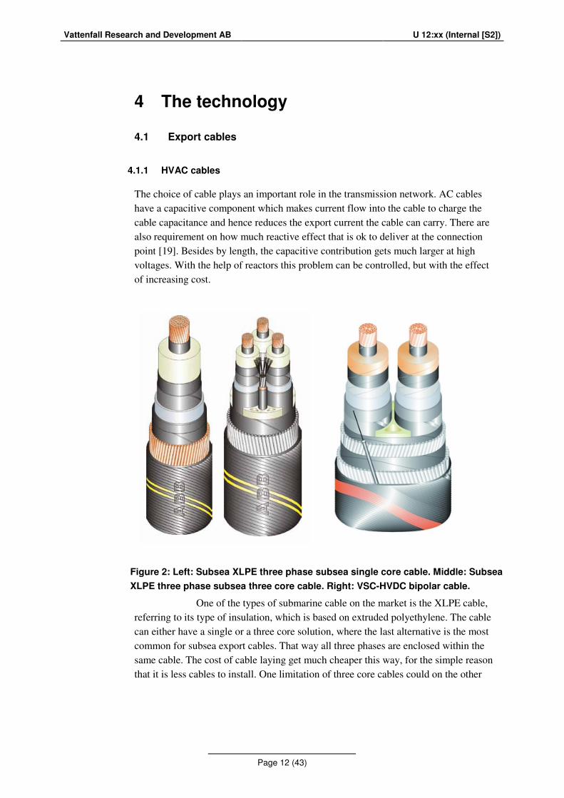
One of the types of submarine cable on the market is the XLPE cable, referring to its type of insulation, which is based on extruded polyethylene. The cable can either have a single or a three core solution, where the last alternative is the most common for subsea export cables. That way all three phases are enclosed within the same cable. The cost of cable laying get much cheaper this way, for the simple reason that it is less cables to install. One limitation of three core cables could on the other
Figure 2: Left: Subsea XLPE three phase subsea single core cable. Middle: Subsea
XLPE three phase subsea three core cable. Right: VSC-HVDC bipolar cable.
Vattenfall Research and Development AB U 12:xx (Internal [S2])
Page 13 (43)
hand be the larger size, which makes it more difficult to handle. A picture on the two types of cable in intersections can be found to the left and middle in Figure 2.
For land transmission single core cables are more commonly used because of the bigger restriction of transporting big and heavy cable drums compared to what can be done offshore. That way the number of joints will be reduced. Land usage can be a problem though since a lot of space is required. Since the cross section area is not as important here, the cheaper aluminum cables are often used instead of copper as in sea cables.
4.1.2 HVDC cables
Along with the improvement with HVAC technology, the HVDC alternatives keep on developing. Depending on the insulation type the upper limit of the cables are a bit different. With the same insulation type as for the AC cables, XLPE, the upper limit is ± 320 kV allowing 500 MW per pole. With other types of insulation the limit is higher, but with reduced cost and benefits like comparative ease of jointing, making manufacturers active developing the XLPE HVDC cables. Another common type of insulation, both for HVDC and HVAC is mass impregnated insulation (MIND). A picture of a MIND HVDC cable is shown to the right in Figure 2. With cable joints required approximately every 750 m onshore, the higher cost and difficulties of jointing, MIND cables is not an alternative for larger distances [20].
4.2 Sea laying
There are many difficulties when it comes to subsea cable installations, some of them depending on the site, like depth of water and type of seabed. Other factors are more dependent on the physics of the cable, like minimum bending radius for wrapping on a wire drum and weight, for the ability to carry as much cable as possible on a vessel. For smaller cables, as those in the internal network of the wind farm, it is possible to use barges to lay the cable, but when the dimensions of cables get bigger special sea laying vessels are needed. Just a few of these large vessels exists and can by that imply a problem with availability. A reason for why a maximum cable length is preferred is because of the jointing of the cable. Good weather during many days is required for this process, at first just to be able to leave the harbor, but then during the operation time where at least one of the cable are hanging down from the vessel, putting the crew to risk if the waves are higher than a few meters.
Vattenfall Research and Development AB U 12:xx (Internal [S2])
Page 14 (43)
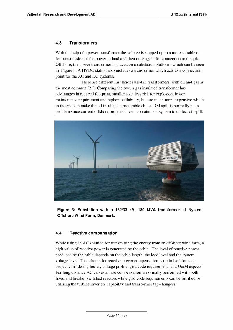
4.3 Transformers
With the help of a power transformer the voltage is stepped up to a more suitable one for transmission of the power to land and then once again for connection to the grid. Offshore, the power transformer is placed on a substation platform, which can be seen in Figure 3. A HVDC station also includes a transformer which acts as a connection point for the AC and DC systems. There are different insulations used in transformers, with oil and gas as the most common [21]. Comparing the two, a gas insulated transformer has advantages in reduced footprint, smaller size, less risk for explosion, lower maintenance requirement and higher availability, but are much more expensive which in the end can make the oil insulated a preferable choice. Oil spill is normally not a problem since current offshore projects have a containment system to collect oil spill.
4.4 Reactive compensation
While using an AC solution for transmitting the energy from an offshore wind farm, a high value of reactive power is generated by the cable. The level of reactive power produced by the cable depends on the cable length, the load level and the system voltage level. The scheme for reactive power compensation is optimized for each project considering losses, voltage profile, grid code requirements and O&M aspects. For long distance AC cables a base compensation is normally performed with both fixed and breaker switched reactors while grid code requirements can be fulfilled by utilizing the turbine inverters capability and transformer tap-changers.
Figure 3: Substation with a 132/33 kV, 180 MVA transformer at Nysted
Offshore Wind Farm, Denmark.

Vattenfall Research and Development AB U 12:xx (Internal [S2])
Page 15 (43)
4.5 Challenges of the transmission network
For realizing the creation of an offshore wind farm there is a need for huge vessels to be able to carry all material, lift the parts on place and host the people working with the construction. The number of vessels of this size is limited and has for a long time been the bottle neck. The availability of vessels is getting better and the new bottle neck is grid integration. There are factors that are big challenges for the transmission network. One factor is that every country has it own system and rules. Other factors of high impact for the project are the cost of delay in manufacturing and cost of lost energy due to down time for the transmission network, since it take so long time to repair. Connecting an offshore platform generating AC with an onshore network supplying AC makes the advantage of a HVAC solution pretty obvious. The disadvantages of such a solution is also very well known when it comes to crossing great distances, like high losses, need of reactive compensation and more cables. For long distances to land, a HVDC solution is getting more suitable to apply with less energy losses and less cable demand, which outweighs the relatively high fixed cost of the HVDC converters. There are still uncertainties about where this break point is, where HVDC is getting less costly than HVAC. It all depends on many variables and what’s included in the study, like lead times, unavailability due to planned and unplanned O&M, if there is redundancy built in the system, just for mentioning a few parameters. In a functional design study for the offshore transmission network for EAONE made by the project firm Sinclair Knight Merz, it can be read that this break point is approximately 90km for a 1000MW development [21]. In this assumption no consideration is taken to the availability, which could extend the break point because of better availability for the HVAC solution. This is because of the higher redundancy, since HVAC solution consists of more cables. Providing that great amount of cables as a HVAC solution requires can be a problem though, since manufacturing them would require about half of the world annual production of high voltage cables, according Åke Larsson, Project Resources UK, Vattenfall AB. Other equipment is generally purchased from much larger transmission and distribution industries which are relatively unconstrained. This is with the exception of high voltage transformers, where delivery times are set by general world demand [23].
Besides getting more economical at long distances, there are other advantages with HVDC technology. It gives the possibility to have a difference in both frequency and voltage at the two sides, enabling variable speed wind turbines and could possibly save a transformer. The direction and magnitude of power can also be controlled. Another advantage is that it doesn’t transmit short circuit current like a HVAC solution, which limits the disruption caused by faults on the other end [22].
A market as young and with a limited experience, there is many challenges with HVDC technology. The competition is very limited for HVDC converter platforms and so also for cables, both HVDC and HVAC cables. That means that if the demand is very high due to many developers planning to build a wind farm,
Vattenfall Research and Development AB U 12:xx (Internal [S2])
Page 16 (43)
the already long lead times will get even longer. Another restriction with HVDC is that the converters are huge. They’re getting smaller per MW, but at the same time wind farms are getting bigger and bigger, which means that they are in the need of very big platforms. Yet there is no standardization between HVDC converters, which lead to lack of compatibility between HVDC converters from different suppliers [25].
The approximated lead times for a project of the grandness treated in this report, are much longer for a HVDC solution and keep getting longer in consultancy with developers. A prolongation of lead time can be severe, since so many actions are dependent on each other and the project being very cost intensive. As an example, installing an offshore HVDC platform requires, according to Åke Larsson, about 700 people and a vessel as big that only two of them exist in the world. These vessels have to be booked 3 years in advance and missing out on that time because of extended lead times makes a big impact on the investment cost. The effect of prolonged lead times could also be dependent on the season. During the winter both the wind speed and the electricity price are higher, which could mean that a delay of about three months could make a bigger damage if located over that period. High wind speed also makes the work offshore impossible, delaying it even more.
Connecting as much power as an offshore wind farm can generate is not always possible to the grid close to shore. The network there is not designed as an injection point and therefore needs to be reinforced. Many big investments in other reinforcements of the electric network are already planned though by TSOs, taking up resources [25]. The reason for why a hybrid solution is being simulated is to see how the advantage of a HVAC solution with a faster commissioning together with lower energy losses of a HVDC solution will affect the results. As written in section 3.2.4 the generated energy is affected more by longer lead times than the costs, so an earlier commission could give a positive effect. Another reason for choosing a hybrid solution could be if the date of the first energy is produced would be of importance, like if the old renewable obligation system in UK would be preferred to use, since it is to be changed 2018.
5 Simulations of transmission alternatives
5.1 About EeFarm II
EeFarm II is a simulation software for making technical and economic calculations for offshore wind farms. The software uses the interface of Matlab and Simulink, together with its own library. The model is built in Simulink by putting blocks together, blocks that can be found in the EeFarm library and represent one component in the wind farm, for example a wind turbine, a transformer or a cable segment. For making the model easier to work with, blocks can be created to represent for example a platform including all the components.

Vattenfall Research and Development AB U 12:xx (Internal [S2])
Page 17 (43)
When a model of the wind farm is made in Simulink, it is necessary to define technical information for all components, but also availability and economical parameters. This is specified most favorable in the already existing Matlab files, which will be loaded while simulating. It is of course possible to write new Matlab files for this, but the easiest way is to copy an old model that work, together with its Matlab files and remodel it to fit the new model. A database consisting of an m-file with technical and some economic data for the components has been designed, but is mostly just used for technical specification of cables and rectifier/inverter in these models. The advantage of using the database is that all parameters needed for making a simulation is specified there.
For a given wind distribution, a power curve for the turbine and all parameters above, nine outputs are created at every component - voltage, current, phase angles for voltage and current, power, reactive power, active power losses, power losses due to availability and investment cost. This information in transferred to the next block and updated by the calculations made inside the components. For analyzing the results, an output converter can be added to the model. This should be done in the end of the model, but could also be added in between two blocks for analyzing and comparing results at a certain place in the network.
With the help of postprocessor files, the results of the simulation can be compiled and evaluated. The result includes power production depending on wind speed, power losses, annual energy production and LCOE (Euro/MWh).
To put the model together in Simulink is quite easy, where a good manual explaining all components also exist. Understanding how to use Matlab together with it can be more of a problem though, since many people have been working with the files in Matlab and multiple languages has been used for commenting the files, if the comments at all exists. One restriction with EeFarm II is that to at all be able to do the simulation, very specific technical information such as resistance, conductivity, mutual inductance in windings, should be defined. Many of these factors are not yet available, since many components will be designed to fit that specific case. Together with many uncertainties in the inputs, the benefit of very specific input data gets lost. It also demands that you know a lot about the technique behind transmission of offshore wind power and by that not for everyone to use. Another limitation with the software is that it doesn’t account for the possibility to transmit a part of the power via neighboring cables during time with less wind and the cables are not fully used. It doesn’t originally include downtime due to planned O&M either. Further, the calculations of LCOE do not include lead times, which will be shown later on, has a big impact on the metric. In the following models, this has been solved by making calculations from the output data in Excel.
With knowledge about offshore wind power and EeFarm II, making models is easy and not very time demanding, giving the possibility to easily compare many alternatives for transmitting energy from offshore wind farms.
Vattenfall Research and Development AB U 12:xx (Internal [S2])
Page 18 (43)
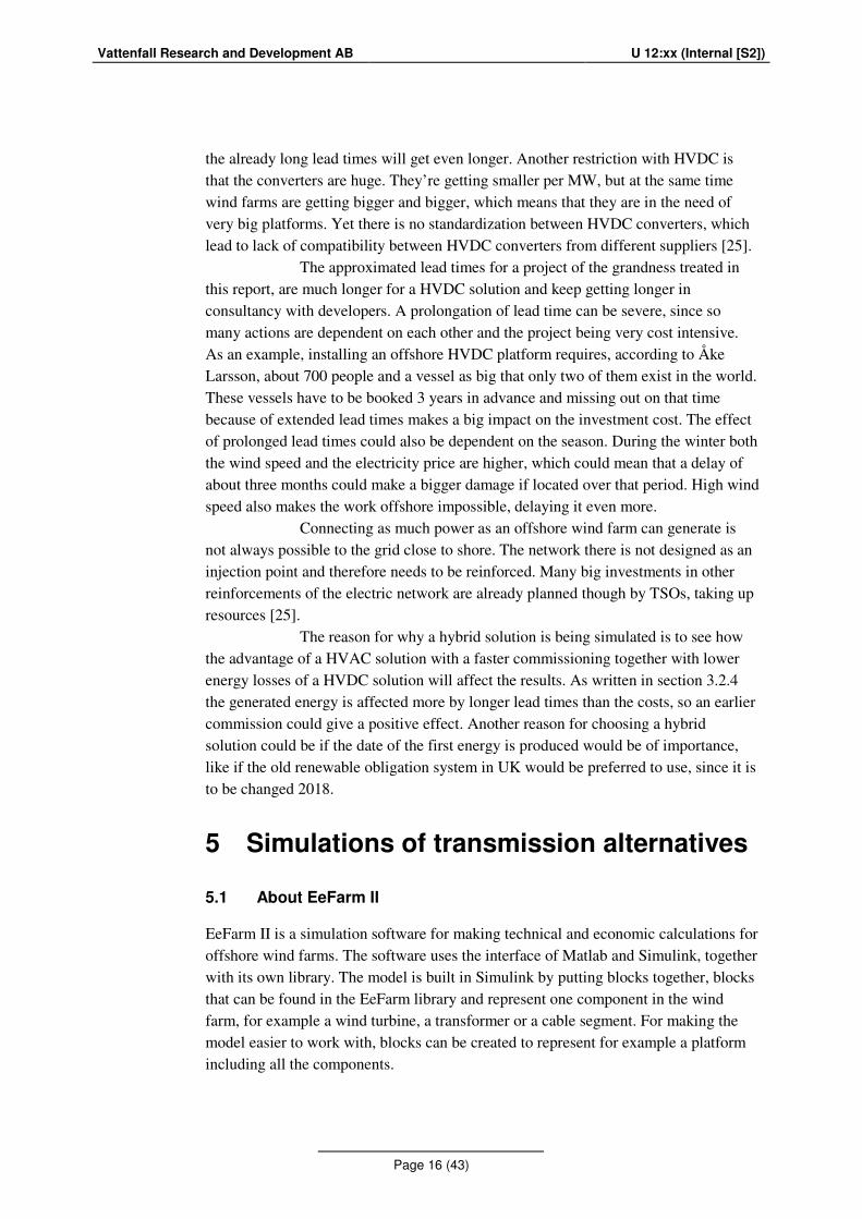
5.2 Background for modeling
Wind data for the simulations have been taken from measurements at the site of the future farm and can be seen in Figure 4 together with the power curve of the turbines and the energy production. The values have been divided into bins of 0.1 m/s. With a cut in speed for the wind turbines at 4 m/s, the site has 8110 production hours yearly and an average wind speed of 10.2 m/s.
Investment cost are taken from calculations made by Thomas Davy, Pöyry, with a background from an existing farm, Thanet, and O&M costs (both planned and unplanned) estimated by Francois Besnard, Development Manager, Vattenfall AB, based on offers for wind farms with HVAC systems. The investment and O&M costs are specified in Appendix F and G. Availability factors are provided by He Ying, Power System Analysis, Vattenfall AB with specifications found in Appendix H. Decommissioning cost and redundancy are not included in these models.
Figure 4: (a): Amount of hours over a year with a 0.1 m/s wind speed
spectra. (b): Yearly energy production divided over 0.1 m/s wind speed
spectres. (c): Power generated at a certain wind speed.
Vattenfall Research and Development AB U 12:xx (Internal [S2])
Page 19 (43)
5.3 HVAC model
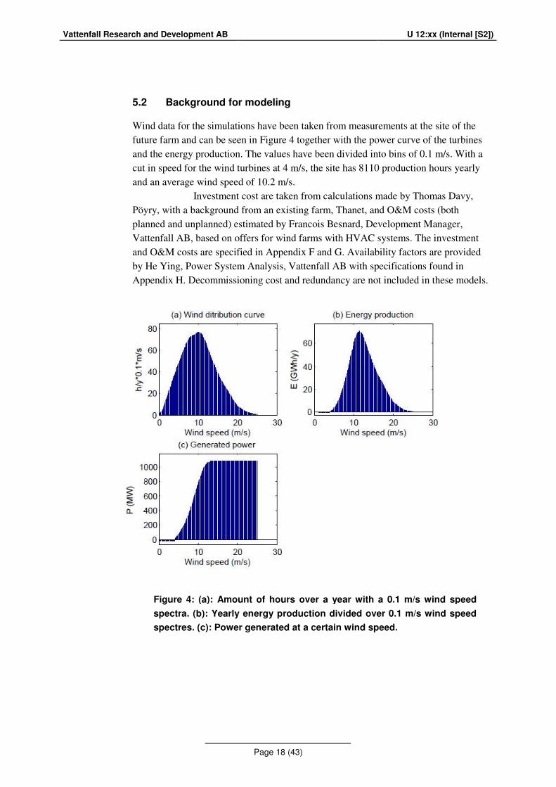
A model is made with the same technical input data as an AC feasibility study made of EAONE in the electric transmission software PSS/E [12], where the grid code requirements for the UK grid where to be fulfilled. Present requirement is a zero exchange of reactive power at the connection point. The whole transmission is divided into three identical parts for limitations in transmitting the power. The proposed reactive power compensation scheme can be seen in Figure 5.
Since the design of the wind farm is not to be considered here, the wind
farm is simplified as 6 equal turbines each of 200 MW (which for the reader could be translated to around 30 large turbines in reality). The price and failure rate of the turbines and intra array network is both put to zero for full focus on the transmission network. For each 400 MW part, the two turbines are connected to two transformers on an offshore platform, where the voltage is stepped up from 33 to 150 kV. Two separate 3-phase 3-core cables transport the energy to shore, where the electricity is transmitted by 1-core cables. A transformer steps up the voltage to 400 kV at Bramford, which is required for connection to the grid. The same reactive power compensation scheme as proposed in [12] is used, with two 70 Mvar reactors placed on the offshore platform and two more at Bramford, together with three 53 Mvar reactors that can be switched on if needed, i.e. when the power supply from the wind farm is very low. More specified technical information can be shown in Table 1 below.
70 Mvar
70 Mvar70 Mvar
70 Mvar
3x53 Mvar
400 kV 150 kV33 kV
BramfordOffshore
150 kV
land cable submarine cable
Figure 5: Proposed reactive power compensation scheme for the AC feasibility study
used as a background

Vattenfall Research and Development AB U 12:xx (Internal [S2])
Page 20 (43)
Table 1: Technical specification for the components included in each 400 MW part
Cables Size R [Ω/km] C [µH] L [mF] Length [km]
3-core Cu sea cable 1 200 mm2
0,047 0,24 0,350 180
1-core Al land cable 1 200 mm2
0,046 0,24 0,382 70
Transformers Rating R X Pieces
Transformer 150/33 kV, 240 MVA 0,5 % 15 % 2
Transformer 400/150 kV, 480 MVA 0,5 % 15 % 1
Reactors Rating Pieces
Offshore shunt reactor 70 Mvar 2
Onshore shunt reactor 70 Mvar 2
Onshore shunt reactor, breaker switched 53 Mvar 3
A picture over how the model is built in EeFarm II is seen in Figure 6.
This model consists of 8 main blocks for each 400 MW part, with a more complicated structure inside them for including all components. Normally the radial block have a line of wind turbines inside them, but as mentioned before they are replaced by one big, and therefore the radials below just includes one wind turbine each. The offshore platform PF12 exists of two platform-blocks, for adding the investment cost in the program, two transformers and two reactors. Under the sea cable mask there is 10 identical blocks, representing a cable part of 9 km. A similar solution is done for the land cable with 5 blocks representing a 7 km cable part. This is for comparing the results with a similar study made in PSS/E.
Figure 6: EeFarm II model of HVAC transmission network for a 400 MW part
of the park
Vattenfall Research and Development AB U 12:xx (Internal [S2])
Page 21 (43)
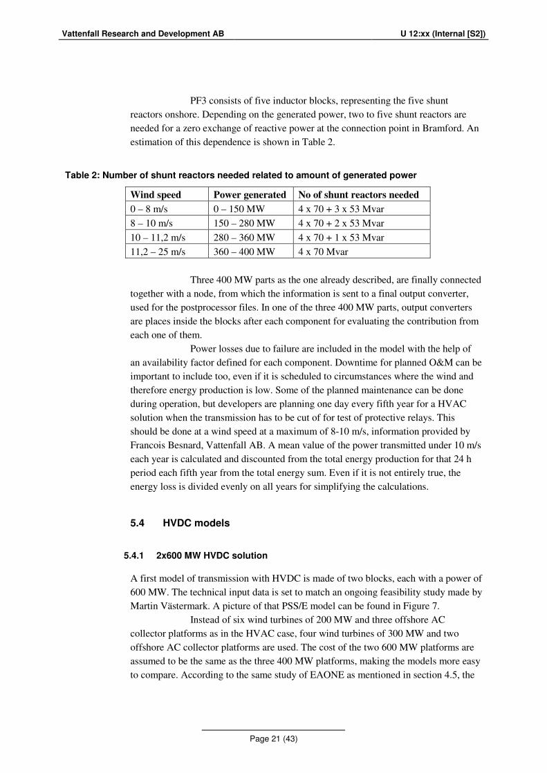
PF3 consists of five inductor blocks, representing the five shunt reactors onshore. Depending on the generated power, two to five shunt reactors are needed for a zero exchange of reactive power at the connection point in Bramford. An estimation of this dependence is shown in Table 2.
Table 2: Number of shunt reactors needed related to amount of generated power
Wind speed Power generated No of shunt reactors needed
0 – 8 m/s 0 – 150 MW 4 x 70 + 3 x 53 Mvar 8 – 10 m/s 150 – 280 MW 4 x 70 + 2 x 53 Mvar 10 – 11,2 m/s 280 – 360 MW 4 x 70 + 1 x 53 Mvar 11,2 – 25 m/s 360 – 400 MW 4 x 70 Mvar
Three 400 MW parts as the one already described, are finally connected together with a node, from which the information is sent to a final output converter, used for the postprocessor files. In one of the three 400 MW parts, output converters are places inside the blocks after each component for evaluating the contribution from each one of them.
Power losses due to failure are included in the model with the help of an availability factor defined for each component. Downtime for planned O&M can be important to include too, even if it is scheduled to circumstances where the wind and therefore energy production is low. Some of the planned maintenance can be done during operation, but developers are planning one day every fifth year for a HVAC solution when the transmission has to be cut of for test of protective relays. This should be done at a wind speed at a maximum of 8-10 m/s, information provided by Francois Besnard, Vattenfall AB. A mean value of the power transmitted under 10 m/s each year is calculated and discounted from the total energy production for that 24 h period each fifth year from the total energy sum. Even if it is not entirely true, the energy loss is divided evenly on all years for simplifying the calculations.
5.4 HVDC models
5.4.1 2x600 MW HVDC solution
A first model of transmission with HVDC is made of two blocks, each with a power of 600 MW. The technical input data is set to match an ongoing feasibility study made by Martin Västermark. A picture of that PSS/E model can be found in Figure 7. Instead of six wind turbines of 200 MW and three offshore AC collector platforms as in the HVAC case, four wind turbines of 300 MW and two offshore AC collector platforms are used. The cost of the two 600 MW platforms are assumed to be the same as the three 400 MW platforms, making the models more easy to compare. According to the same study of EAONE as mentioned in section 4.5, the
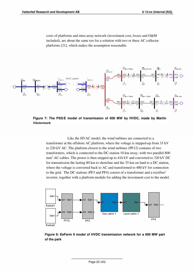
Vattenfall Research and Development AB U 12:xx (Internal [S2])
Page 22 (43)
costs of platforms and intra array network (investment cost, losses and O&M included), are about the same too for a solution with two or three AC collector platforms [21], which makes the assumption reasonable.
Like the HVAC model, the wind turbines are connected to a
transformer at the offshore AC platform, where the voltage is stepped-up from 33 kV to 220 kV AC. The platform closest to the wind turbines (PF12) contains of two transformers, which is connected to the DC-station 10 km away, with two parallel 800 mm2 AC-cables. The power is then stepped up to 416 kV and converted to 320 kV DC for transmission the lasting 80 km to shoreline and the 35 km on land to a DC station, where the voltage is converted back to AC and transformed to 400 kV for connection to the grid. The DC stations (PF3 and PF4) consist of a transformer and a rectifier/ inverter, together with a platform module for adding the investment cost to the model.
Figure 8: EeFarm II model of HVDC transmission network for a 600 MW part
of the park
Figure 7: The PSS/E model of transmission of 600 MW by HVDC, made by Martin
Västermark
Vattenfall Research and Development AB U 12:xx (Internal [S2])
Page 23 (43)
Cable data for the AC cable is provided by Per-Olof Lindström. The
technical data for the HVDC solution is matched to an, for the time of this thesis, ongoing study made by Martin Västermark and can be found in Table 3. This is with exception for the transformer at the DC-station onshore, which is set to X = 0.15 % instead of X = 0 % for minimizing the reactive power out of the transformer and transmitted to the connection point. A HVDC light station can be set to not deliver any reactive power, which is not the case for the model in EeFarm II and why it has to be compensated this way. Active losses are around 1 % for a HVDC-light station [25], which in EeFarm II is already lost in the rectifier and inverter modules with the input data available. Because of that, the resistances of the transformers on these platforms are put to zero. Specifications for the DC cables are found in EeFarm’s library, but resistance for 20ºC can also be confirmed by numbers on ABB’s webpage [26].
Time for planned O&M is much longer for a HVDC solution than a HVAC solution, and is expected to be about 7-10 days/year by developers for shutting down the converters. In this simulations, a mean time of 8,5 days is used for calculation losses. Like the HVAC solution, the mean power transmitted under a wind speed of 10 m/s is used in the calculations.
Table 3: Technical specification for the components included in each 600 MW part
AC cable Size R C L Length
3-core Cu sea cable 800 mm2
0,0221 Ω 0,17 µH 0,40 mF 2 x 10 km
DC cable Size R 20ºC R 90ºC Length
HVDC light cable, bipolar 630 mm2
0,0283 Ω 0,0360 Ω 80 + 35 km
Transformers Rating R X Pieces
Transformer 220/33 kV, 330 MVA 0,5 % 15 % 2
Transformer 416/220 kV, 845 MVA 0 % 14 % 1
Transformer 400/416 kV, 845 MVA 0 % 0.15 % 1
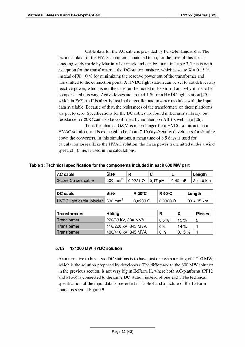
5.4.2 1x1200 MW HVDC solution
An alternative to have two DC stations is to have just one with a rating of 1 200 MW, which is the solution proposed by developers. The difference to the 600 MW solution in the previous section, is not very big in EeFarm II, where both AC-platforms (PF12 and PF56) is connected to the same DC-station instead of one each. The technical specification of the input data is presented in Table 4 and a picture of the EeFarm model is seen in Figure 9.
Vattenfall Research and Development AB U 12:xx (Internal [S2])
Page 24 (43)
Table 4: Technical specification for the components included in the 1200 MW solution
AC cable Size R C L Length
3-core Cu sea cable 800 mm2
0,055 Ω 0,17 µH 0,40 mF 4 x 10 km
DC cable Size R 20ºC R 90ºC Length
HVDC light cable, bipolar 2000 mm2
0,009 Ω 0,011 Ω 80+35 km
Transformers Rating R X Pieces
Transformer 220/33 kV, 330 MVA 0,5 % 15 % 4
Transformer 416/220 kV, 1690 MVA 0 % 14 % 1
Transformer 400/416 kV, 1690 MVA 0 % 0.15 % 1
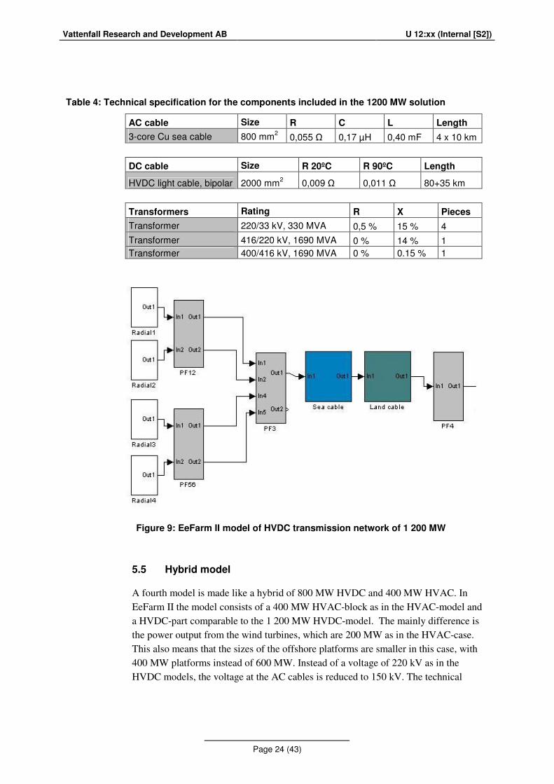
5.5 Hybrid model
A fourth model is made like a hybrid of 800 MW HVDC and 400 MW HVAC. In EeFarm II the model consists of a 400 MW HVAC-block as in the HVAC-model and a HVDC-part comparable to the 1 200 MW HVDC-model. The mainly difference is the power output from the wind turbines, which are 200 MW as in the HVAC-case. This also means that the sizes of the offshore platforms are smaller in this case, with 400 MW platforms instead of 600 MW. Instead of a voltage of 220 kV as in the HVDC models, the voltage at the AC cables is reduced to 150 kV. The technical
Figure 9: EeFarm II model of HVDC transmission network of 1 200 MW
Vattenfall Research and Development AB U 12:xx (Internal [S2])
Page 25 (43)
specification of the input data is the same for the HVAC-block in section 5.3, while the data for the HVDC-block is modified and presented in Table 5. A picture of the EeFarm model is seen in Figure 10.
Table 5: Technical specification for the components included in the 800 MW HVDC part
AC cable Size R C L Length
3-core Cu sea cable 800 mm2
0,055 Ω 0,17 µH 0,40 mF 4 x 10 km
DC cable Size R 20ºC R 90ºC Length
HVDC light cable, bipolar 1200 mm2
0,0151 Ω 0,019 Ω 80+35 km
Transformers Rating R X Pieces
Transformer 150/33 kV, 330 MVA 0,5 % 15 % 4
Transformer 416/150 kV, 1690 MVA 0 % 14 % 1
Transformer 400/416 kV, 1690 MVA 0 % 0.15 % 1
Figure 10: EeFarm II model of a hybrid solution with transmission via 400 MW HVAC
and 800 MW HVDC
Vattenfall Research and Development AB U 12:xx (Internal [S2])
Page 26 (43)
Power losses for planned O&M are calculated by the same values as for the other models – 1 day every fifth year for a third of the farm and 8,5 days for the rest of it, all with a maximum wind speed of 10 m/s.
5.6 Economic models
5.6.1 Economic parameters
Information about price of electricity and ROCs are provided by Tobias Johansson, OEDP, Vattenfall AB. Since the transmission network itself doesn’t produce any energy and is just a part of a bigger system, it would not be correct to use the full revenues made for the electricity. In consultation with Åke Larsson, Project Resources UK, Vattenfall AB, the transmission network stands for 25 % of the total investment cost, for which reason a fourth of the revenues have been used in the calculations for IRR and NPV. Input data for the economic models have been excluded in the report, as it is confidential information.
A lifetime of 20 years has been used in these models, calculated from commissioning. With different time of commissioning for different parts of the farm means that they will also have different times of decommissioning.
One simplification done in the economic model of the hybrid solution is that energy losses and O&M is not divided by type on transmission solution being in commission, which means that a differ in these values could affect the result slightly, since the HVAC part is being commissioned before the HVDC part.
5.6.2 Lead time
Lead times, i.e. the time it takes from signing a contract with the developer until the farm is ready to deliver energy, is an important factor to put into the models. For this HVAC model a lead time for a 400 MW part of the farm is estimated, in consultation with Åke Larsson, to be 36 months. The second and third part is estimated to be in commission after additionally 6 and 12 moths. Estimating a lead time for a HVDC solution of this size is very hard, and keeps getting longer in consultations with developers. Once again, the technology is very new and has been fairly used in projects even close to this size. The best estimation, for the moment of publishing this thesis, is 57 months, independent of size of the converter station. This means that it takes the same time to put a 600 MW, 800 MW or 1200 MW HVDC solution in commission. The second part of the two-platform-solution is estimated to be ready for commission a year later, giving the solution a total lead time of 69 months.
Vattenfall Research and Development AB U 12:xx (Internal [S2])
Page 27 (43)
5.6.3 Pay plan
The economic models are done in Excel with input data from the simulations done in EeFarm II. The investment cost is divided into yearly payments distributed over the lead time, divided proportionally to a graph with payments over time, distributed by Siemens. This draft was made for a 1 GW HVDC solution with two platforms for EAONE and can be found in Appendix E. Payments for the different solutions are estimated to be proportional to the graph, having a starting cost of 14,3 % of the investment cost. O&M cost are then added as a percentage of total capacity installed. Besides Levelized Cost Of Energy, the Net Price Value and Internal Rate of Return is calculated for all models.
6 Result
The results of the four simulations are being summarized in Table 6and Table 7, the first with produced energy and energy losses and the second with economical metrics. As mentioned before, a HVAC solution has higher active losses, which also can be concluded by looking at Table 6, while energy losses due to failure are bigger for the HVDC solutions. Totally the HVDC solution with one platform has least energy losses and the other HVDC solution second least losses, closely followed though by the hybrid solution. The CF is higher than normal in this study, since losses in the wind turbines and intra array network are not included.
The HVDC solution with one DC platform also has the lowest investment cost, which has a background that it’s a more optimized solution by the suppliers, compared to the two platform solution. The specification of the costs and power losses will be presented later on in this section.
Table 6: Modeling results for the four models, produced energy and energy losses
HVAC HVDC 1 HVDC 2 Hybrid
Average power generation [MW] 656 668 671 665
CF 54,68% 55,69% 55,90% 55,43%
AUE [GWh/y] 5 739 5 789 5 812 5 780
Active energy losses 6,00% 3,60% 3,24% 4,28%
Energy losses due to failure 3,97% 4,73% 4,74% 4,48%
No load losses 0,13% 0,03% 0,02% 0,06%
Losses due to planned O&M 0,02% 0,99% 0,99% 0,66%
Total losses 10,13% 9,34% 8,99% 9,48%
Vattenfall Research and Development AB U 12:xx (Internal [S2])
Page 28 (43)
Table 7: Modeling results for the four models, economical parameters
HVAC HVDC 1 HVDC 2 Hybrid
Investment cost [M€] 1 095 1 196 989 1 124
Total O&M cost [M€/y] 10,54 23,93 19,99 18,20
Total costs, discounted [M€] 992 1084 925 1035
LCOE [€/MWh] 25,11 31,53 25,71 27,47
IRR 15,32% 12,60% 14,84% 14,33%
NPV [M€] 387,60 76,30 300,76 265,22
Even though as much as 10 % of the power is lost during transmission
with a HVAC solution, the shorter lead time makes the LCOE low compared to the other solutions, even though the one platform solution for HVDC is very close in number. The shorter lead time also gives the HVAC solution the highest IRR and NPV, indicating that it is the most profitable solution
6.1 HVAC model
In Figure 11 a diagram of the specified investment cost for the HVAC solution is presented. The far most expensive part is the sea cable, which stands for more than half of the cost itself and together with the land cable for about 2/3 of the cost. The second biggest cost is the offshore station and its transformers.
Figure 11: Costs for a HVAC solution, divided on different sections of the
transmission network
Vattenfall Research and Development AB U 12:xx (Internal [S2])
Page 29 (43)
The cables are not just the most expensive part of the transmission network – it is also the part where most of the power losses occur. The sea cable takes much longer to repair after a fault because of need of a suitable vessel and an appropriate weather window, which can be seen in Figure 12 by the big difference in availability for sea and land cables. Power losses in the cable have been compared to a PSS/E study of same structure [19], where the differences are pretty small - 79,9 kW/km to 82,2 kW/km for sea cable and 83,9 kW/km to 82,9 kW/km for land cable, which means that the power losses for the cable in this model should be close to reality.
6.2 HVDC models
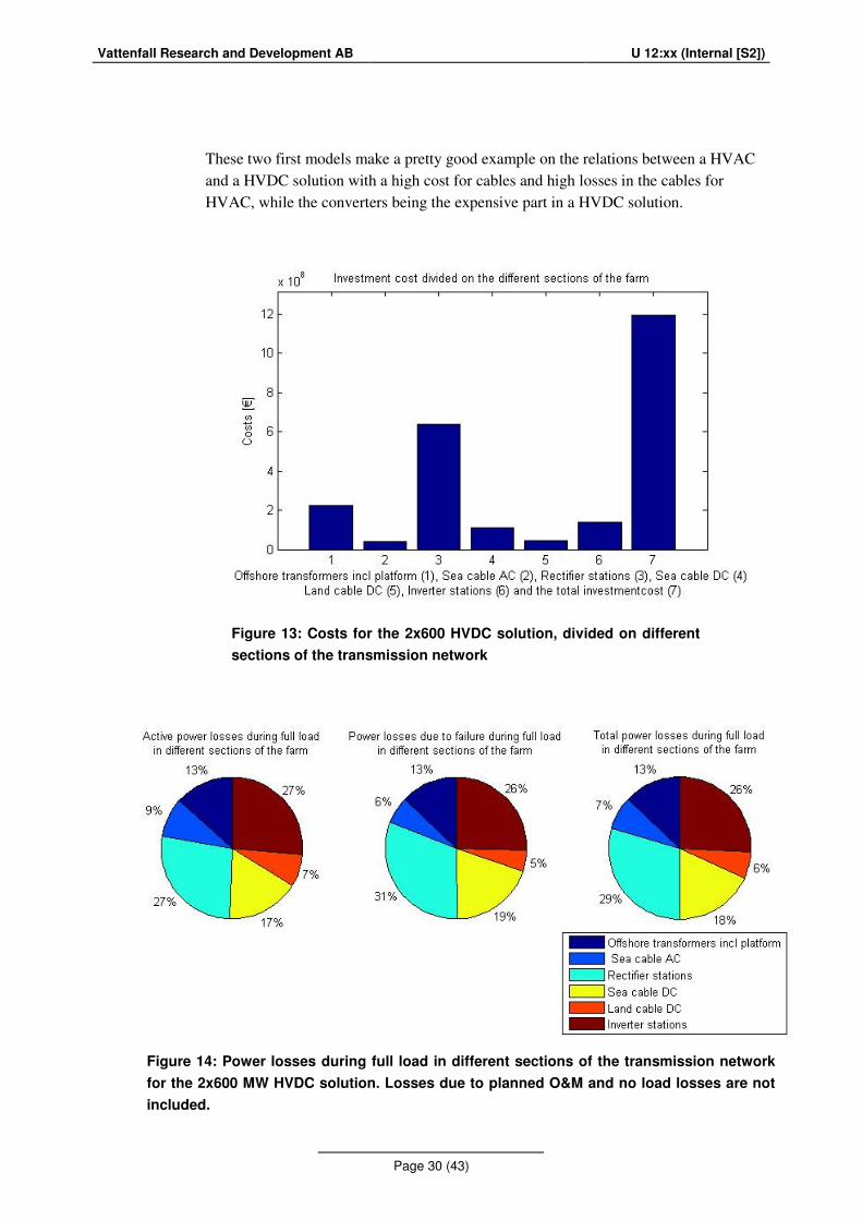
6.2.1 2x600 MW HVDC solution
Instead of a high cable cost, like the previous model, the biggest investment here is the rectifier station with its platform, where the rectifier itself is about a third as expensive as the platform it stands on.
As for the losses, they are more even distributed than in the HVAC model with the big losses in the converters, even though the DC cables have pretty high losses too.
Figure 12: Power losses during full load in different sections of the transmission network
for the HVAC solution. Losses due to planned O&M and no load losses are not included.
Vattenfall Research and Development AB U 12:xx (Internal [S2])
Page 30 (43)
These two first models make a pretty good example on the relations between a HVAC and a HVDC solution with a high cost for cables and high losses in the cables for HVAC, while the converters being the expensive part in a HVDC solution.
Figure 13: Costs for the 2x600 HVDC solution, divided on different
sections of the transmission network
Figure 14: Power losses during full load in different sections of the transmission network
for the 2x600 MW HVDC solution. Losses due to planned O&M and no load losses are not
included.

Vattenfall Research and Development AB U 12:xx (Internal [S2])
Page 31 (43)
6.2.2 1x1200 MW HVDC solution
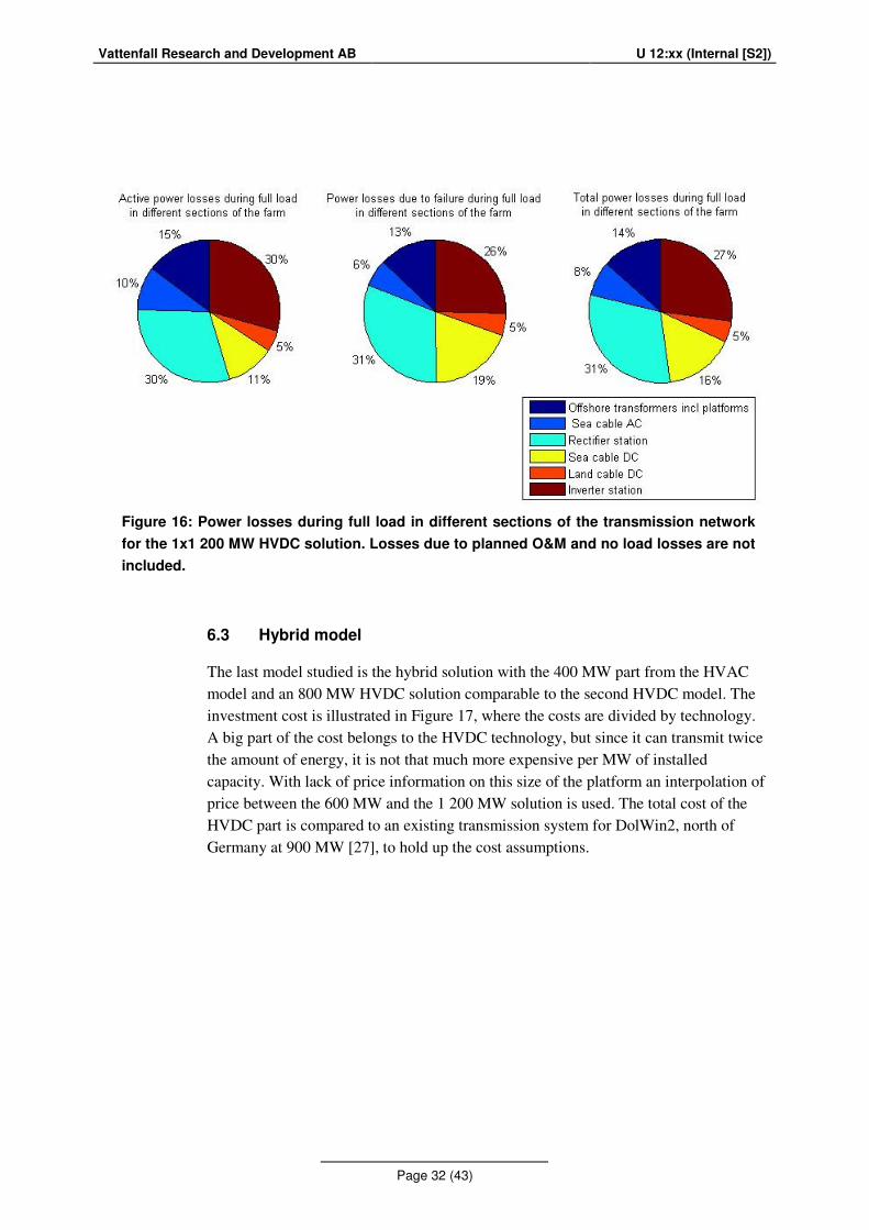
With just one HVDC platform the total cost of the HVDC technology gets lower for a reason of fewer cables and platforms, but also with a cheaper converter station per MW installed. The redundancy of the system gets very poor though, since a failure in the HVDC technology would mean that the whole production gets lost. The power losses for this model are very close to the other HVDC model, since the active power losses are controlled to be as close as possible to 1 % of the rated power (as explained in 5.4.1), which makes it difficult to compare them.
Figure 15: Costs for the 1x1200 HVDC solution, divided on different sections of the
transmission network
Vattenfall Research and Development AB U 12:xx (Internal [S2])
Page 32 (43)
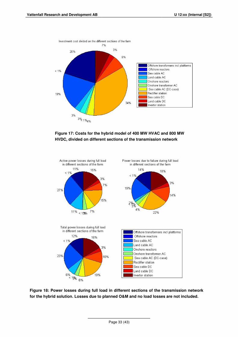
6.3 Hybrid model
The last model studied is the hybrid solution with the 400 MW part from the HVAC model and an 800 MW HVDC solution comparable to the second HVDC model. The investment cost is illustrated in Figure 17, where the costs are divided by technology. A big part of the cost belongs to the HVDC technology, but since it can transmit twice the amount of energy, it is not that much more expensive per MW of installed capacity. With lack of price information on this size of the platform an interpolation of price between the 600 MW and the 1 200 MW solution is used. The total cost of the HVDC part is compared to an existing transmission system for DolWin2, north of Germany at 900 MW [27], to hold up the cost assumptions.
Figure 16: Power losses during full load in different sections of the transmission network
for the 1x1 200 MW HVDC solution. Losses due to planned O&M and no load losses are not
included.
Vattenfall Research and Development AB U 12:xx (Internal [S2])
Page 33 (43)
Figure 18: Power losses during full load in different sections of the transmission network
for the hybrid solution. Losses due to planned O&M and no load losses are not included.
Figure 17: Costs for the hybrid model of 400 MW HVAC and 800 MW
HVDC, divided on different sections of the transmission network
Vattenfall Research and Development AB U 12:xx (Internal [S2])
Page 34 (43)
The mixes of technology result in total power losses a bit higher than the HVDC solutions, but lower than the HVAC solution. With the possibility to generate energy much faster than a HVDC solution, the discounted value of power transmitted by the hybrid solution gets higher, but a high investment cost gives the hybrid solution a higher LCOE than both the HVAC and second HVDC solution.
6.4 Sensitivity analysis
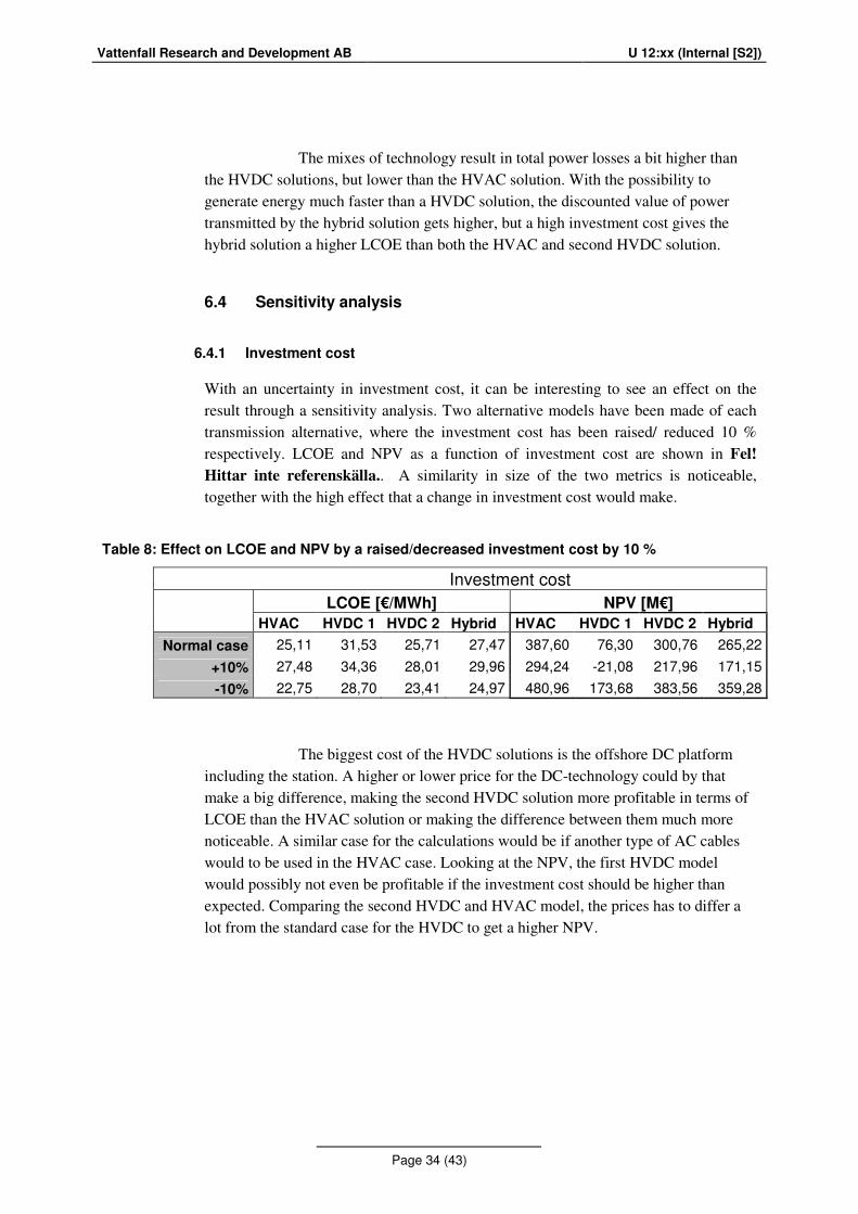
6.4.1 Investment cost
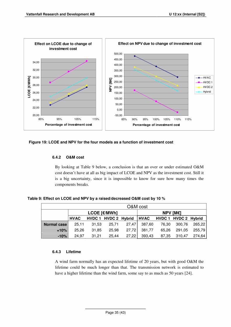
With an uncertainty in investment cost, it can be interesting to see an effect on the result through a sensitivity analysis. Two alternative models have been made of each transmission alternative, where the investment cost has been raised/ reduced 10 % respectively. LCOE and NPV as a function of investment cost are shown in Fel!
Hittar inte referenskälla.. A similarity in size of the two metrics is noticeable, together with the high effect that a change in investment cost would make.
Table 8: Effect on LCOE and NPV by a raised/decreased investment cost by 10 %
Investment cost
LCOE [€/MWh] NPV [M€]
HVAC HVDC 1 HVDC 2 Hybrid HVAC HVDC 1 HVDC 2 Hybrid
Normal case 25,11 31,53 25,71 27,47 387,60 76,30 300,76 265,22
+10% 27,48 34,36 28,01 29,96 294,24 -21,08 217,96 171,15
-10% 22,75 28,70 23,41 24,97 480,96 173,68 383,56 359,28
The biggest cost of the HVDC solutions is the offshore DC platform including the station. A higher or lower price for the DC-technology could by that make a big difference, making the second HVDC solution more profitable in terms of LCOE than the HVAC solution or making the difference between them much more noticeable. A similar case for the calculations would be if another type of AC cables would to be used in the HVAC case. Looking at the NPV, the first HVDC model would possibly not even be profitable if the investment cost should be higher than expected. Comparing the second HVDC and HVAC model, the prices has to differ a lot from the standard case for the HVDC to get a higher NPV.
Vattenfall Research and Development AB U 12:xx (Internal [S2])
Page 35 (43)
6.4.2 O&M cost
By looking at Table 9 below, a conclusion is that an over or under estimated O&M cost doesn’t have at all as big impact of LCOE and NPV as the investment cost. Still it is a big uncertainty, since it is impossible to know for sure how many times the components breaks.
Table 9: Effect on LCOE and NPV by a raised/decreased O&M cost by 10 %
O&M cost
LCOE [€/MWh] NPV [M€]
HVAC HVDC 1 HVDC 2 Hybrid HVAC HVDC 1 HVDC 2 Hybrid
Normal case 25,11 31,53 25,71 27,47 387,60 76,30 300,76 265,22
+10% 25,26 31,85 25,98 27,72 381,77 65,26 291,05 255,79
-10% 24,97 31,21 25,44 27,22 393,43 87,35 310,47 274,64
6.4.3 Lifetime
A wind farm normally has an expected lifetime of 20 years, but with good O&M the lifetime could be much longer than that. The transmission network is estimated to have a higher lifetime than the wind farm, some say to as much as 50 years [24].
Figure 19: LCOE and NPV for the four models as a function of investment cost
Effect on LCOE due to change of
investment cost
20,00
22,00
24,00
26,00
28,00
30,00
32,00
34,00
85% 95% 105% 115%
Percentage of investment cost
LC
OE
[€/M
Wh
]
Effect on NPV due to change of investment cost
-50,00
0,00
50,00
100,00
150,00
200,00
250,00
300,00
350,00
400,00
450,00
500,00
85% 90% 95% 100% 105% 110% 115%
Percentage of investment cost
NP
V [
M€] HVAC
HVDC 1
HVDC 2
Hybrid

Vattenfall Research and Development AB U 12:xx (Internal [S2])
Page 36 (43)
An extended lifetime certainly makes the LCOE lower for all cases but don’t change the difference between the solutions that much. The differences in NPV between the models are about the same too for the two extra cases.
Table 10: Effect on LCOE and NPV by an extended lifetime to 25 and 30 years
Lifetime
LCOE [€/MWh] NPV [M€]
HVAC HVDC 1 HVDC 2 Hybrid HVAC HVDC 1 HVDC 2 Hybrid
n=20 25,11 31,53 25,71 27,47 387,60 76,30 300,76 265,22
n=25 23,38 29,42 24,10 25,97 463,66 136,75 361,46 319,72
n=30 22,37 28,19 23,08 24,86 508,79 172,63 400,02 360,92
6.4.4 Unavailability
Like cost of O&M, a change in the availability of transmission network doesn’t seem to affect the values very much, but is a factor with higher risk since it is based on passed event and the few farms of these sizes are very young and the background data is poor.
Table 11: Effect on LCOE and NPV by a raised/decreased unavailability by 10 %
Unavailability
LCOE [€/MWh] NPV [M€]
HVAC HVDC 1 HVDC 2 Hybrid HVAC HVDC 1 HVDC 2 Hybrid
Normal case 25,11 31,53 25,71 27,47 387,60 76,30 300,76 265,22
+10% 25,22 31,69 25,83 27,60 381,63 70,45 294,96 258,97
-10% 25,00 31,37 25,59 27,33 393,59 82,18 306,58 271,49
6.4.5 Capacity factor
Different wind conditions than measured could be a possibility, either with more accurate measurements or just as a yearly variation, which could affect the profitability of the project. Two extra modulations on each transmission alternative have been done where the CF has been raised/ decreased by 10 %. A change in wind speed seem to highly affect the result, as can be seen in Table 12, but not so much the difference in result of the four models.
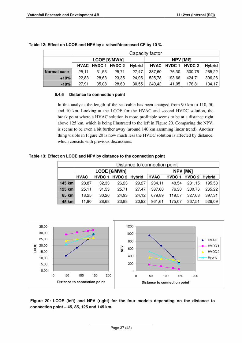
Vattenfall Research and Development AB U 12:xx (Internal [S2])
Page 37 (43)
Table 12: Effect on LCOE and NPV by a raised/decreased CF by 10 %
Capacity factor
LCOE [€/MWh] NPV [M€]
HVAC HVDC 1 HVDC 2 Hybrid HVAC HVDC 1 HVDC 2 Hybrid
Normal case 25,11 31,53 25,71 27,47 387,60 76,30 300,76 265,22
+10% 22,83 28,63 23,35 24,95 525,78 193,66 424,71 396,26
-10% 27,91 35,08 28,60 30,55 249,42 -41,05 176,81 134,17
6.4.6 Distance to connection point
In this analysis the length of the sea cable has been changed from 90 km to 110, 50 and 10 km. Looking at the LCOE for the HVAC and second HVDC solution, the break point where a HVAC solution is more profitable seems to be at a distance right above 125 km, which is being illustrated to the left in Figure 20. Comparing the NPV, is seems to be even a bit further away (around 140 km assuming linear trend). Another thing visible in Figure 20 is how much less the HVDC solution is affected by distance, which consists with previous discussions.
Table 13: Effect on LCOE and NPV by distance to the connection point
Distance to connection point
LCOE [€/MWh] NPV [M€]
HVAC HVDC 1 HVDC 2 Hybrid HVAC HVDC 1 HVDC 2 Hybrid
145 km 28,87 32,33 26,23 29,27 234,11 48,54 281,15 195,53
125 km 25,11 31,53 25,71 27,47 387,60 76,30 300,76 265,22
85 km 18,25 30,26 24,93 24,12 679,89 119,57 327,68 397,31
45 km 11,90 28,68 23,88 20,92 961,61 175,07 367,51 526,09
Figure 20: LCOE (left) and NPV (right) for the four models depending on the distance to
connection point – 45, 85, 125 and 145 km.
0
200
400
600
800
1000
1200
0 50 100 150 200
Distance to connection point
NP
V
HVAC
HVDC 1
HVDC 2
Hybrid
0,00
5,00
10,00
15,00
20,00
25,00
30,00
35,00
0 50 100 150 200
Distance to connection point
LC
OE
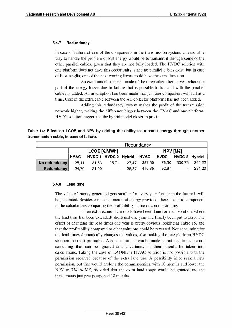
Vattenfall Research and Development AB U 12:xx (Internal [S2])
Page 38 (43)
6.4.7 Redundancy
In case of failure of one of the components in the transmission system, a reasonable way to handle the problem of lost energy would be to transmit it through some of the other parallel cables, given that they are not fully loaded. The HVDC solution with one platform does not have this opportunity, since no parallel cables exist, but in case of East Anglia, one of the next coming farms could have the same function.
An extra model has been made of the three other alternatives, where the part of the energy losses due to failure that is possible to transmit with the parallel cables is added. An assumption has been made that just one component will fail at a time. Cost of the extra cable between the AC collector platforms has not been added. Adding this redundancy system makes the profit of the transmission network higher, making the difference bigger between the HVAC and one-platform-HVDC solution bigger and the hybrid model closer in profit.
Table 14: Effect on LCOE and NPV by adding the ability to transmit energy through another
transmission cable, in case of failure.
Redundancy
LCOE [€/MWh] NPV [M€]
HVAC HVDC 1 HVDC 2 Hybrid HVAC HVDC 1 HVDC 2 Hybrid
No redundancy 25,11 31,53 25,71 27,47 387,60 76,30 300,76 265,22
Redundancy 24,70 31,09 - 26,87 410,85 92,67 - 294,20
6.4.8 Lead time
The value of energy generated gets smaller for every year further in the future it will be generated. Besides costs and amount of energy provided, there is a third component in the calculations comparing the profitability - time of commissioning. Three extra economic models have been done for each solution, where the lead time has been extended/ shortened one year and finally been put to zero. The effect of changing the lead times one year is pretty obvious looking at Table 15, and that the profitability compared to other solutions could be reversed. Not accounting for the lead times dramatically changes the values, also making the one-platform-HVDC solution the most profitable. A conclusion that can be made is that lead times are not something that can be ignored and uncertainty of them should be taken into calculations. Taking the case of EAONE, a HVAC solution is not possible with the permission received because of the extra land use. A possibility is to seek a new permission, but that would prolong the commissioning with 18 months and lower the NPV to 334,94 M€, provided that the extra land usage would be granted and the investments just gets postponed 18 months.
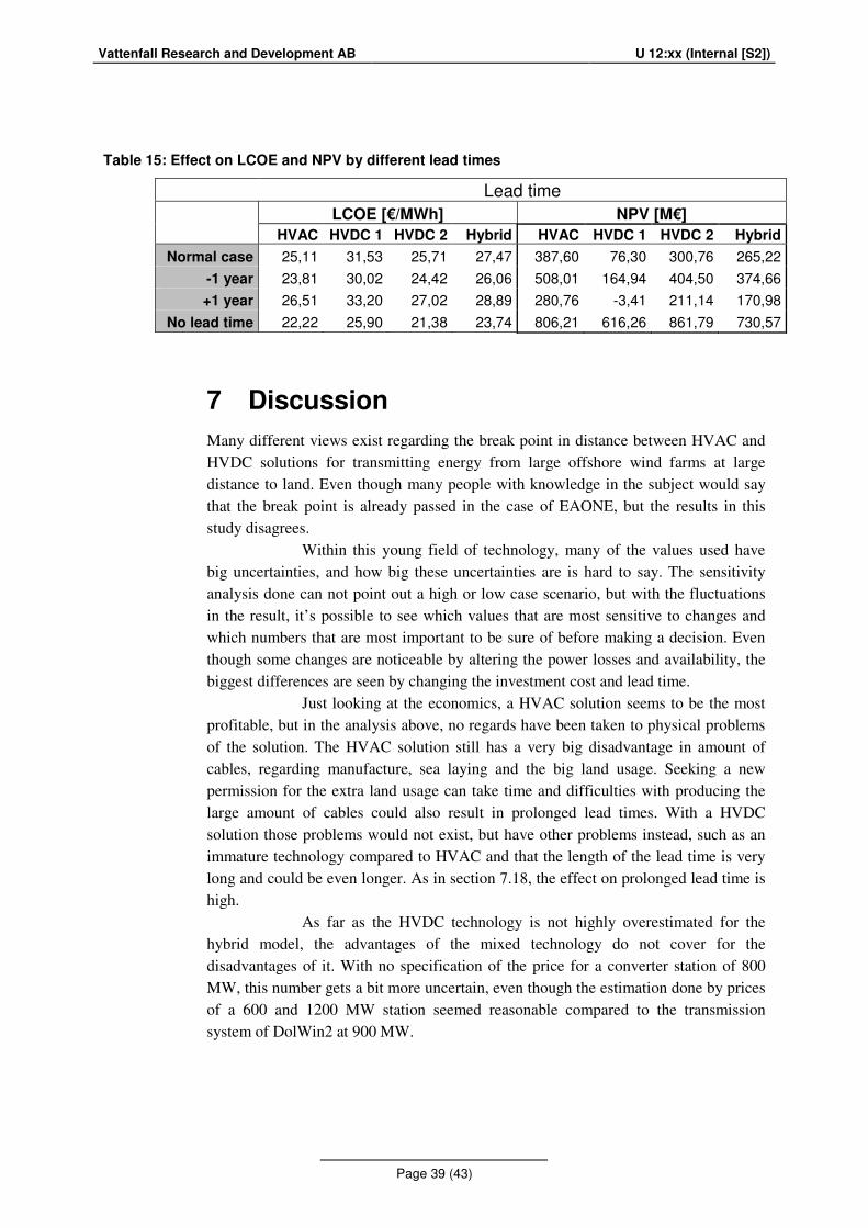
Vattenfall Research and Development AB U 12:xx (Internal [S2])
Page 39 (43)
Table 15: Effect on LCOE and NPV by different lead times
Lead time
LCOE [€/MWh] NPV [M€]
HVAC HVDC 1 HVDC 2 Hybrid HVAC HVDC 1 HVDC 2 Hybrid
Normal case 25,11 31,53 25,71 27,47 387,60 76,30 300,76 265,22
-1 year 23,81 30,02 24,42 26,06 508,01 164,94 404,50 374,66
+1 year 26,51 33,20 27,02 28,89 280,76 -3,41 211,14 170,98
No lead time 22,22 25,90 21,38 23,74 806,21 616,26 861,79 730,57
7 Discussion
Many different views exist regarding the break point in distance between HVAC and HVDC solutions for transmitting energy from large offshore wind farms at large distance to land. Even though many people with knowledge in the subject would say that the break point is already passed in the case of EAONE, but the results in this study disagrees.
Within this young field of technology, many of the values used have big uncertainties, and how big these uncertainties are is hard to say. The sensitivity analysis done can not point out a high or low case scenario, but with the fluctuations in the result, it’s possible to see which values that are most sensitive to changes and which numbers that are most important to be sure of before making a decision. Even though some changes are noticeable by altering the power losses and availability, the biggest differences are seen by changing the investment cost and lead time.
Just looking at the economics, a HVAC solution seems to be the most profitable, but in the analysis above, no regards have been taken to physical problems of the solution. The HVAC solution still has a very big disadvantage in amount of cables, regarding manufacture, sea laying and the big land usage. Seeking a new permission for the extra land usage can take time and difficulties with producing the large amount of cables could also result in prolonged lead times. With a HVDC solution those problems would not exist, but have other problems instead, such as an immature technology compared to HVAC and that the length of the lead time is very long and could be even longer. As in section 7.18, the effect on prolonged lead time is high.
As far as the HVDC technology is not highly overestimated for the hybrid model, the advantages of the mixed technology do not cover for the disadvantages of it. With no specification of the price for a converter station of 800 MW, this number gets a bit more uncertain, even though the estimation done by prices of a 600 and 1200 MW station seemed reasonable compared to the transmission system of DolWin2 at 900 MW.
Vattenfall Research and Development AB U 12:xx (Internal [S2])
Page 40 (43)
For upcoming projects much closer to land, a HVAC link should be used with its economic advantage seen in the sensitivity analysis, as long as land usage is not a problem. In some years, as the market of HVDC grows, bringing down the prices and speeding up the manufacturing, a HVDC solution at a distance similar to EAONE would probably be a more economical solution. With investment costs and lead times as for this models and provided that a HVAC transmission network for a wind farm like EAONE is feasible, a HVAC solution should be considered and further investigated. With a NPV still higher than the HVDC solution after a delay of the project with 18 months and depending how it would affect the total project of East Anglia, a HVAC solution could even be reasonable for EAONE.
8 Conclusions
Four models have been made in EeFarm II with complementing calculations in Excel. A sensitivity analysis has also been made for analyzing the influence on LCOE and NPV made by a change in some input parameters. From the result of this study, following were concluded:
• A HVAC solution is the most economical with input data used in the simulations, but has technical disadvantages in the great amount of cables required.
• The disadvantages of a hybrid solution seem to be bigger than the advantages, making it less economical than both a HVAC and a HVDC solution.
• Investment cost and lead time has a big influence on the result, which means that a HVDC solution could be cheaper in the future because of development in the HVDC market, making the prices lower and shorter manufacturing time.
• The difference in NPV and LCOE between the HVAC and HVDC model is widely affected by distance to land, making the HVAC model a much more economical solution for shorter distances.
9 Acknowledgements
There are many people that I would like to thank for their support and constant willingness to help, that wouldn’t make it possible to make this thesis to what it is.
Firstly, I would like to thank my main supervisor at Vattenfall, Urban Axelsson for his big support, encouragement and contribution with knowledge in the subject. I would also like to thank my secondary supervisor Tobias Johansson, for his valuable inputs and spending all the time helping me understand EeFarm II, and my other secondary supervisor Pernilla Ove for sharing her experience in the field. Speaking of EeFarm II, I would like to express my great appreciation to Jan Pierik, ECN, for answering my question and checking some of my invalid models.
Vattenfall Research and Development AB U 12:xx (Internal [S2])
Page 41 (43)
The estimation in availability made by Ying He and input from Francois Besnard about availability and O&M have been very valuable and I really appreciate the time they spent on it, even though they had loads of work to do themselves. Besides information from people here at Vattenfall in Solna, I would like to send my thanks to three persons at Vattenfall in London – Åke Larsson, Honor Green and Clare MacGregor, for the shared knowledge in transmission network, the economics behind it and last but not least, their grand patience.
My supervisor at Umeå universitet, Björne Lindberg, has been a big support during the thesis too and should have a special thank for that.
On a personal level, I would like to thank the other thesis writers at Vattenfall R&D, Martin Västermark and Emil Hagström, for making the days at Vattenfall even better.
10 References
[1] “Wind Energy FAQ”, EWEA. [online] Available: http://www.ewea.org/wind-energy-basics/wind-energy-faq/ [Retrieved: Jan 15th 2013]
[2] “Offshore wind energy – news, facts and events”, EWEA. [online] Available: http://www.ewea.org/news/detail/?tx_ttnews%5Btt_news%5D=556&cHash=b894641208aaf61351badd4c16419321 [Retrieved: Jan 15th 2013]
[3] European Wind Energy Association, “Wind in our Sails”, 2011. [PDF] Available: http://www.ewea.org/fileadmin/files/library/publications/reports/Offshore_Report.pdf [Retrieved: Jan 15th 2013]
[4] “London Eye”, Wikipedia. [online] Available: http://en.wikipedia.org/wiki/London_Eye [Retrieved: Jan 15th 2013]
[5] “Close up – the E126, still the world’s biggest turbine”, Wind power
monthly. [online] http://www.windpowermonthly.com/news/1138562/Close---E126-worlds-biggest-turbine/ [Retrieved: Jan 15th 2013]
[6] “Statue of Liberty”, Wikipedia. [online] Available: http://en.wikipedia.org/wiki/Statue_of_Liberty [Retrieved: Jan 15th 2013]
[7] “Elanvändning”, Svensk Energi. [online] http://www.svenskenergi.se/sv/Om-el/Elanvandning/ [Retrieved: Jan 15th 2013]
[8] S. Krohn, “The economics of wind energy”, European Wind Energy Association, March 2009. [PDF] Available: http://www.ewea.org/fileadmin/ewea_documents/documents/00_POLICY_document/Economics_of_Wind_Energy__March_2009_.pdf [Retrieved: Nov 26th 2013]
Vattenfall Research and Development AB U 12:xx (Internal [S2])
Page 42 (43)
[9] “Vindkraft – en viktig del av framtidens kraftsystem”, Svensk
Energi.[online] http://www.svenskenergi.se/sv/Vi-arbetar-med/Elproduktion/Vindkraft/ [Retrieved: Jan 15th 2013]
[10] “Planning our electric future: technical update”, Department of Energy &
Climate change. [PDF] Available: http://www.decc.gov.uk/assets/decc/11/meeting-energy-demand/energy-markets/3884-planning-electric-future-technical-update.pdf [Retrieved: Jan 15th 2013]
[11] C. Kolliatsas, Mott MacDonald, “Risk, Mitigation and Cost Reduction”, Offshore Wind Economics & Finance, London 2012. [PDF]
[12] R. Helms, DONG Energy, “Introduction to DONG Energy Wind Power”, Offshore Wind Economics & Finance, London 2012. [PDF]
[13] M. van der Heijden, Typhoon Offshore, “What drives equity investors in offshore wind?”, Offshore Wind Economics & Finance, London 2012. [PDF]
[14] Tande, J. and R. Hunter, “Estimation of Cost of Energy from Wind Energy Conversion Systems”, Recommended practices for wind turbine testing, 2nd edition. IEA, 1994. [PDF] Available: http://www.ieawind.org/mwg-internal/de5fs23hu73ds/progress?id=lxNgw8kEid [Retrieved: Oct 25th 2012]
[15] S. Özer, “A Feasibility Study and Evaluation of Financing Models for Wind Energy Projects”, A Case Study on Izmir Institute of Technology Campus
Area, July 2004. [PDF] Available: http://www.ieawind.org/mwg-internal/de5fs23hu73ds/progress?id=lxNgw8kEid [Retrieved: Oct 25th 2012]
[16] A. Beddard, Dr. M. Barnes, ”VSC-HVDC Availability Analysis”, The University of Manchester, Revision 2.0, November 2011. [PDF]
[17] C. Jones, “Optimization Of Number Of Collector Platforms”, Functional
Design Specification for Zone Transmission Network Contract, , v.2, 27 June 2011 [PDF]
[18] S. Krohn, “The economics of wind energy”, European Wind Energy Association, March 2009. [PDF] Available: http://www.ewea.org/fileadmin/ewea_documents/documents/00_POLICY_document/Economics_of_Wind_Energy__March_2009_.pdf [Retrieved: Oct 25th 2012]
[19] P. Lindström, H. Wiesbach, AC Study of East Anglia Offshore Wind 1, 16 July 2012. [PDF]
[20] “Appendix one, Offshore Development Information Statement Appendices”, 2009. [PDF]
[21] C. Jones, “Technology Report”, Functional Design Specification for Zone
Transmission Network Contract, , v.3, 18 May 2011. [PDF] [22] S. Wright, “Transmission options for offshore wind farms in the United
States”, Renewable Energy Research Lab, University of Massachusetts.
[PFD] Available: http://ceere.org/rerl/publications/published/2002/Transmission_Options_For
Vattenfall Research and Development AB U 12:xx (Internal [S2])
Page 43 (43)
_Offshore_Wind_Farms_In_The_US,_AWEA_June_2002_.pdf [Retrieved: Oct 25th 2012]
[23] “Appendix four, Offshore Development Information Statement Appendices”, 2009. [PDF]
[24] B. Goethals, elia group, “The challenges of offshore wind integration”, Offshore Wind Economics & Finance, London 2012. [PDF]
[25] G. Persson, “HVDC Converter Operations and Performance, Classic and VSC”, 18 Sep 2011 [PDF]. Available: http://www.sari-energy.org/mwg-internal/de5fs23hu73ds/progress?id=jGTyZC0jCh [Retrieved: Jan 15th 2013]
[26] ABB, ”XLPE Land Cable Systems”, User’s Guide, Rev 5. [PDF] Available: http://www05.abb.com/global/scot/scot245.nsf/veritydisplay/ab02245fb5b5ec41c12575c4004a76d0/$file/xlpe%20land%20cable%20systems%202gm5007gb%20rev%205.pdf [Retrieved: Jan 15th 2013]
[27] “HC 517 The Economics of Wind Power”, UK Parliament, June 2012, [online]. Available: http://www.publications.parliament.uk/pa/cm201213/cmselect/cmenergy/writev/517/m08.htm [Retrieved: Jan 15th 2012]
10.1 Pictures
Figure 1: Left: http://www.abb.com/product/db0003db002618/c12573e7003302adc125702e0055084a.aspx Right: http://www.modernpowersystems.com/storyprint.asp?sc=2050430
Figure 2: http://193.88.185.141/Graphics/Publikationer/Havvindmoeller/kap09.htm
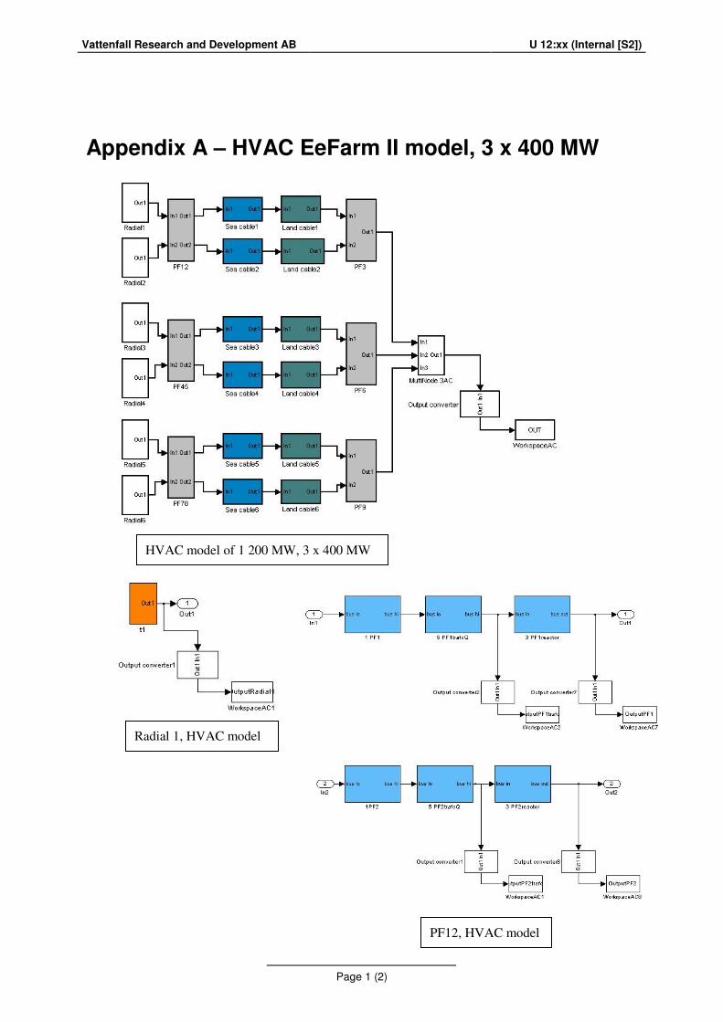
Vattenfall Research and Development AB U 12:xx (Internal [S2])
Page 1 (2)
Appendix A – HVAC EeFarm II model, 3 x 400 MW
Radial 1, HVAC model
HVAC model of 1 200 MW, 3 x 400 MW
PF12, HVAC model

Vattenfall Research and Development AB U 12:xx (Internal [S2])
Page 2 (2)
Sea cable, HVAC model
PF3, HVAC model
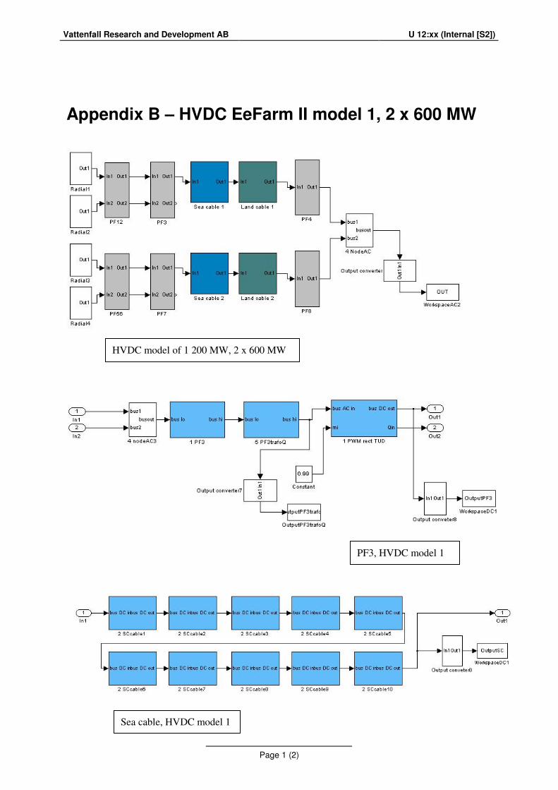
Vattenfall Research and Development AB U 12:xx (Internal [S2])
Page 1 (2)
Appendix B – HVDC EeFarm II model 1, 2 x 600 MW
HVDC model of 1 200 MW, 2 x 600 MW
PF3, HVDC model 1
Sea cable, HVDC model 1
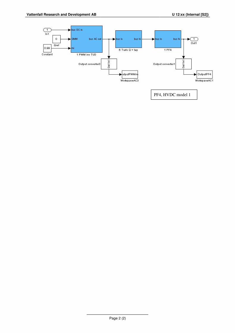
Vattenfall Research and Development AB U 12:xx (Internal [S2])
Page 2 (2)
PF4, HVDC model 1

Vattenfall Research and Development AB U 12:xx (Internal [S2])
Page 1 (1)
Appendix C – HVDC EeFarm II model 2, 1 x 1 200 MW
PF3, HVDC model 2
HVDC model of 1 200 MW, 1 x 1 200 MW
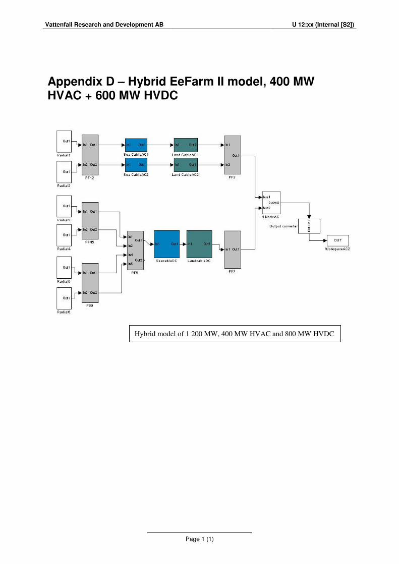
Vattenfall Research and Development AB U 12:xx (Internal [S2])
Page 1 (1)
Appendix D – Hybrid EeFarm II model, 400 MW HVAC + 600 MW HVDC
Hybrid model of 1 200 MW, 400 MW HVAC and 800 MW HVDC

Vattenfall Research and Development AB U 12:xx (Internal [S2])
Page 1 (1)
Appendix E – Pay plan
(Confidential)

Vattenfall Research and Development AB U 12:xx (Internal [S2])
Page 1 (1)
Appendix F – Investment costs
(Confidential)

Vattenfall Research and Development AB U 12:xx (Internal [S2])
Page 1 (1)
Appendix G – O&M cost
(Confidential)

Vattenfall Research and Development AB U 12:xx (Internal [S2])
Page 1 (1)
Appendix H – Availability
(Confidential)