Embed Size (px)
DESCRIPTION
Document detailing the process of Transmission Lines
Citation preview
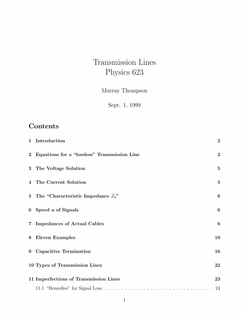
Transmission LinesPhysics 623
Murray Thompson
Sept. 1, 1999
Contents
1 Introduction 2
2 Equations for a “lossless” Transmission Line 2
3 The Voltage Solution 5
4 The Current Solution 5
5 The “Characteristic Impedance Z0” 6
6 Speed u of Signals 6
7 Impedances of Actual Cables 6
8 Eleven Examples 10
9 Capacitive Termination 16
10 Types of Transmission Lines 22
11 Imperfections of Transmission Lines 23
11.1 “Remedies” for Signal Loss . . . . . . . . . . . . . . . . . . . . . . . . . . . . . . 24
1
CONTENTS 2
12 Equations for a “Lossy” Transmission Line 25
13 Lossy Line with No Reflections 29
14 Attenuation if line is slightly lossy 29
15 Characteristic Impedance of a Lossy Transmission Line 30
16 Heavyside Distortionless Lines 30
17 Three Examples 31
18 Attenuation at DC and Low Frequencies 31
19 Attenuation at Higher Frequencies 33
19.1 Skin Effect Loss . . . . . . . . . . . . . . . . . . . . . . . . . . . . . . . . . . . . 33
19.2 Dielectric Loss . . . . . . . . . . . . . . . . . . . . . . . . . . . . . . . . . . . . . 35
19.3 Radiation Loss . . . . . . . . . . . . . . . . . . . . . . . . . . . . . . . . . . . . 35
19.4 Actual Attenuation in Cables . . . . . . . . . . . . . . . . . . . . . . . . . . . . 35
——–
1 INTRODUCTION 3
1 Introduction
A Transmission line is a pair of conductors which have a cross which remains constant withdistance. For example, a coaxial cable transmission line has a cross section of a central rod andan outer concentric cylinder.
Similarly a twisted pair transmission line has two conducting rods or wires which slowlywind around each other. A cross section made at any distance along the line is the same as across section made at any other point on the line.
We want to understand the voltage - Current relationships of transmission lines.
2 Equations for a “lossless” Transmission Line
A transmission line has a distributed inductance on each line and a distributed capacitancebetween the two conductors. We will consider the line to have zero series resistance and theinsulator to have infinite resistance (a zero conductance or perfect insulator). We will considera “Lossy” line later in section 12 on page 25.
Define L to be the inductance/unit length and C to be the capacitance/unit length.
Consider a transmission line to be a pair of conductors divided into a number of cells witheach cell having a small inductance in one line and having small capacitance to the other line.
In the limit of these cells being very small, they can represent a distributed inductance withdistributed capacitance to the other conductor.
Consider one such cell corresponding to the components between position x and positionx+ ∆x along the transmission line.
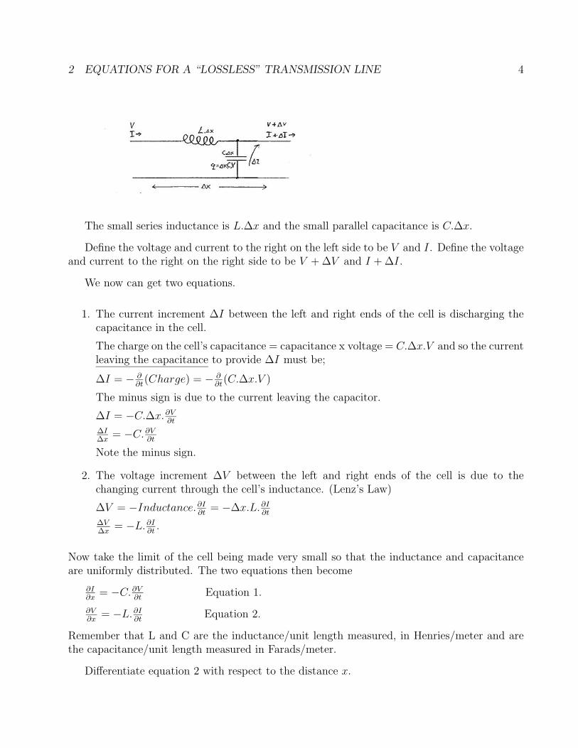
2 EQUATIONS FOR A “LOSSLESS” TRANSMISSION LINE 4
The small series inductance is L.∆x and the small parallel capacitance is C.∆x.
Define the voltage and current to the right on the left side to be V and I. Define the voltageand current to the right on the right side to be V + ∆V and I + ∆I.
We now can get two equations.
1. The current increment ∆I between the left and right ends of the cell is discharging thecapacitance in the cell.
The charge on the cell’s capacitance = capacitance x voltage = C.∆x.V and so the currentleaving the capacitance to provide ∆I must be;
∆I = − ∂∂t
(Charge) = − ∂∂t
(C.∆x.V )
The minus sign is due to the current leaving the capacitor.
∆I = −C.∆x.∂V∂t
∆I∆x
= −C.∂V∂t
Note the minus sign.
2. The voltage increment ∆V between the left and right ends of the cell is due to thechanging current through the cell’s inductance. (Lenz’s Law)
∆V = −Inductance.∂I∂t
= −∆x.L.∂I∂t
∆V∆x
= −L.∂I∂t.
Now take the limit of the cell being made very small so that the inductance and capacitanceare uniformly distributed. The two equations then become
∂I∂x
= −C.∂V∂t
Equation 1.
∂V∂x
= −L.∂I∂t
Equation 2.
Remember that L and C are the inductance/unit length measured, in Henries/meter and arethe capacitance/unit length measured in Farads/meter.
Differentiate equation 2 with respect to the distance x.
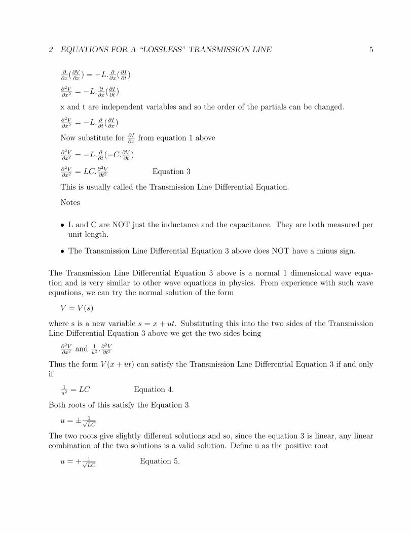
2 EQUATIONS FOR A “LOSSLESS” TRANSMISSION LINE 5
∂∂x
(∂V∂x
) = −L. ∂∂x
(∂I∂t
)
∂2V∂x2 = −L. ∂
∂x(∂I∂t
)
x and t are independent variables and so the order of the partials can be changed.
∂2V∂x2 = −L. ∂
∂t( ∂I∂x
)
Now substitute for ∂I∂x
from equation 1 above
∂2V∂x2 = −L. ∂
∂t(−C.∂V
∂t)
∂2V∂x2 = LC.∂
2V∂t2
Equation 3
This is usually called the Transmission Line Differential Equation.
Notes
• L and C are NOT just the inductance and the capacitance. They are both measured perunit length.
• The Transmission Line Differential Equation 3 above does NOT have a minus sign.
The Transmission Line Differential Equation 3 above is a normal 1 dimensional wave equa-tion and is very similar to other wave equations in physics. From experience with such waveequations, we can try the normal solution of the form
V = V (s)
where s is a new variable s = x + ut. Substituting this into the two sides of the TransmissionLine Differential Equation 3 above we get the two sides being
∂2V∂x2 and 1
u2 .∂2V∂t2
Thus the form V (x+ ut) can satisfy the Transmission Line Differential Equation 3 if and onlyif
1u2 = LC Equation 4.
Both roots of this satisfy the Equation 3.
u = ± 1√LC
The two roots give slightly different solutions and so, since the equation 3 is linear, any linearcombination of the two solutions is a valid solution. Define u as the positive root
u = + 1√LC
Equation 5.
3 THE VOLTAGE SOLUTION 6
3 The Voltage Solution
Thus, the general solution for the voltage is the linear combination.
V = f(x− ut) + g(x+ ut) Equation 6.
Where f() and g() are arbitrary single valued functions which can be very different.
1. f(x− ut) describes a wave propagating with no change in shape towards x = +∞.
2. g(x+ ut) describes a wave propagating with no change in shape towards x = −∞.
4 The Current Solution
Consider one of the waves such as the “forward wave” propagating towards x = +∞.
V = V (x− ut)
From this we can show, by differentiating, that:
−u∂V∂x
= ∂V∂t
∂V∂x
= − 1u.∂V∂t
Equation 7.
Also from equation 2. above
∂V∂x
= −L.∂I∂t
Equation 2.
Equation 2 and equation 7 will have a common solution only if the two right hand sides arethe same
1u.∂V∂t
= L.∂I∂t
V = uL.I
This can be rewritten using u = 1√LC
from equation 5.
V =√
LC.I
and
VI
=√
LC
and the current I of the forward wave is
I = V/√
LC
and, similarly for the backward wave
5 THE “CHARACTERISTIC IMPEDANCE Z0” 7
V = −√
LC.I
VI
= −√
LC
and the current I of the backward wave is
I = −V/√
LC
Thus the general solution for both waves for the current I is
I = (f(x− ut)− g(x+ ut))/√
LC
Equation 7
which can be compared with the earlier equation for the voltage
V = f(x− ut) + g(x+ ut) Equation 6.
5 The “Characteristic Impedance Z0”
Define the “Characteristic Impedance Z0” as the magnitude of the instantaneous ratio for eitherthe forward wave or backward wave. For the forward wave:
Z0 = | V oltageCurrent
| = |VI| = |
√LC|
For the backward wave:
Z0 = | V oltageCurrent
| = |VI| = |
√LC|
With this definition of Z0 the voltage and current equations can be written:
V = f(x− ut) + g(x+ ut) Equation 6.
I = f(x−ut)Z0
− g(x+ut)Z0
Equation 8.
6 Speed u of Signals
The Inductance per unit length L and Capacitance per unit length C can be calculated fromElectromagnetic Theory. The formulae depend upon the cross sectional shape of the conductors.
7 Impedances of Actual Cables
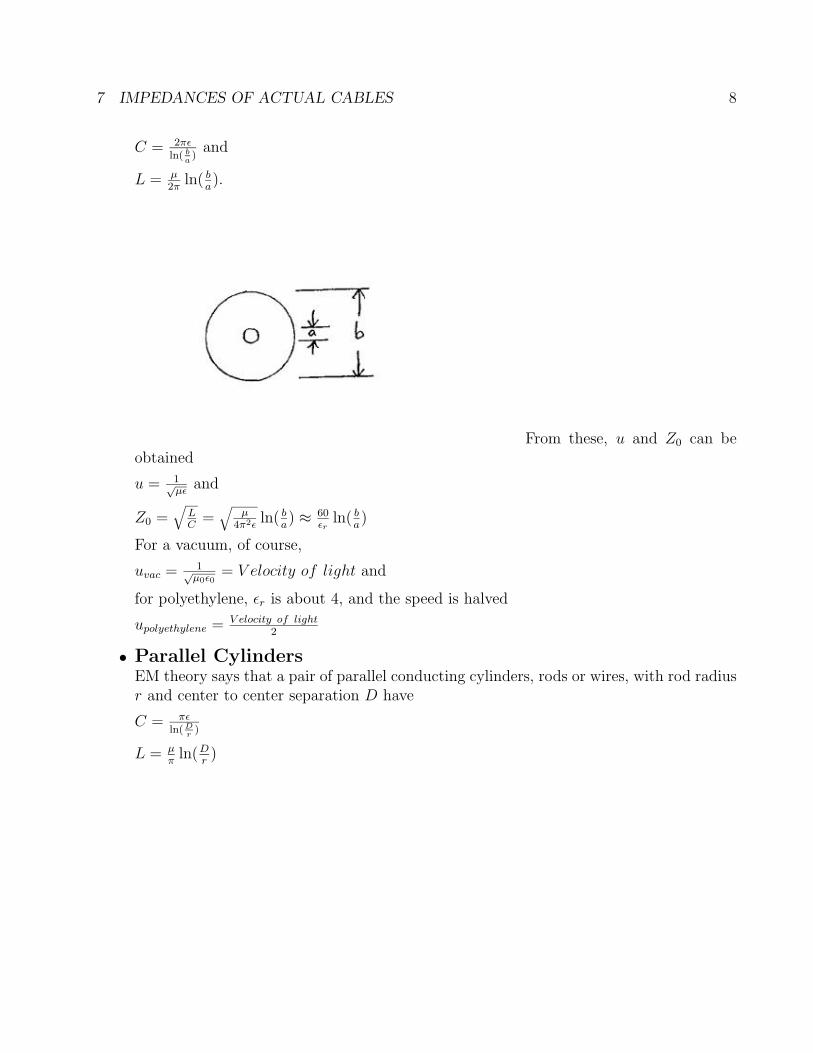
• Coaxial CableEM theory says that a Coaxial Cable with inner rod having diameter a and outer tubehaving diameter b has
7 IMPEDANCES OF ACTUAL CABLES 8
C = 2πεln( b
a)
and
L = µ2π
ln( ba).
From these, u and Z0 can beobtained
u = 1√µε
and
Z0 =√
LC
=√
µ4π2ε
ln( ba) ≈ 60
εrln( b
a)
For a vacuum, of course,
uvac = 1√µ0ε0
= V elocity of light and
for polyethylene, εr is about 4, and the speed is halved
upolyethylene = V elocity of light2
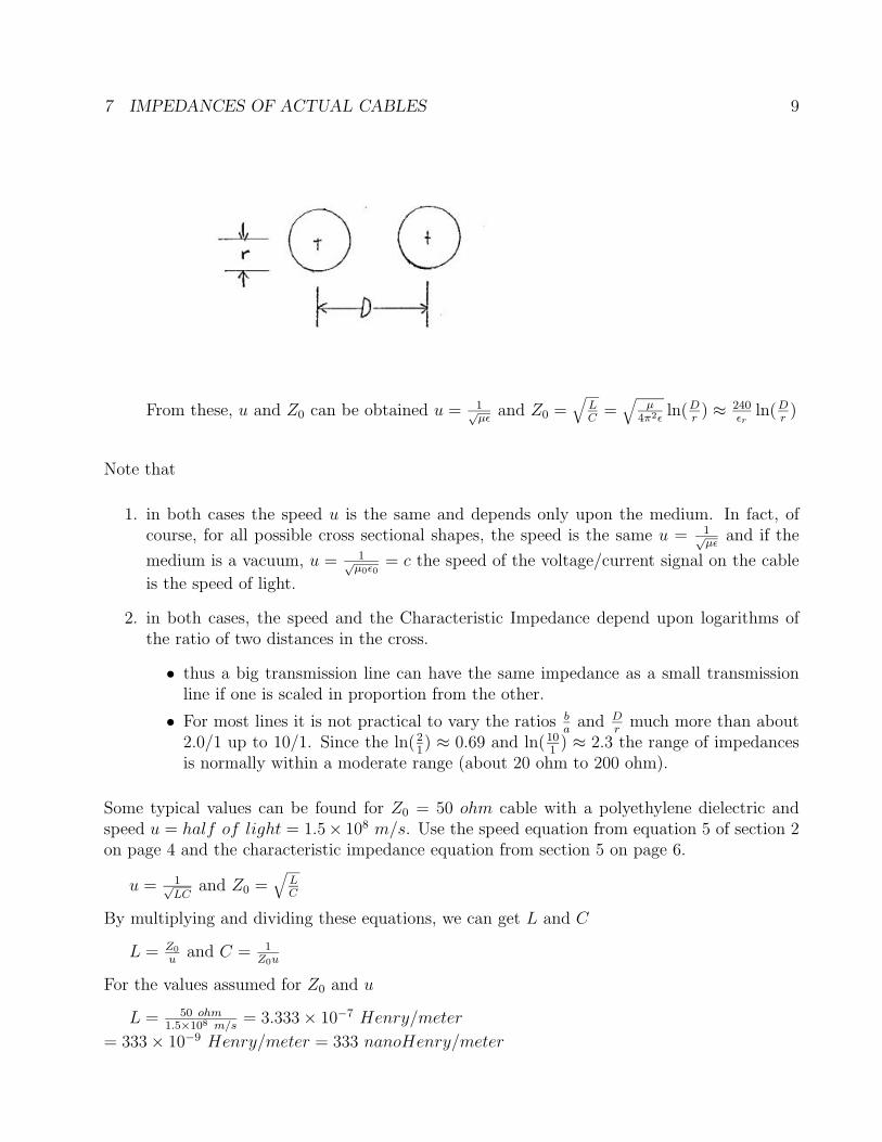
• Parallel CylindersEM theory says that a pair of parallel conducting cylinders, rods or wires, with rod radiusr and center to center separation D have
C = πεln(D
r)
L = µπ
ln(Dr
)
7 IMPEDANCES OF ACTUAL CABLES 9
From these, u and Z0 can be obtained u = 1√µε
and Z0 =√
LC
=√
µ4π2ε
ln(Dr
) ≈ 240εr
ln(Dr
)
Note that
1. in both cases the speed u is the same and depends only upon the medium. In fact, ofcourse, for all possible cross sectional shapes, the speed is the same u = 1√
µεand if the
medium is a vacuum, u = 1√µ0ε0
= c the speed of the voltage/current signal on the cable
is the speed of light.
2. in both cases, the speed and the Characteristic Impedance depend upon logarithms ofthe ratio of two distances in the cross.
• thus a big transmission line can have the same impedance as a small transmissionline if one is scaled in proportion from the other.
• For most lines it is not practical to vary the ratios ba
and Dr
much more than about2.0/1 up to 10/1. Since the ln(2
1) ≈ 0.69 and ln(10
1) ≈ 2.3 the range of impedances
is normally within a moderate range (about 20 ohm to 200 ohm).
Some typical values can be found for Z0 = 50 ohm cable with a polyethylene dielectric andspeed u = half of light = 1.5× 10⁸ m/s. Use the speed equation from equation 5 of section 2on page 4 and the characteristic impedance equation from section 5 on page 6.
u = 1√LC
and Z0 =√
LC
By multiplying and dividing these equations, we can get L and C
L = Z0
uand C = 1
Z0u
For the values assumed for Z0 and u
L = 50 ohm1.5×108 m/s
= 3.333× 10⁻⁷ Henry/meter
= 333× 10−9 Henry/meter = 333 nanoHenry/meter
7 IMPEDANCES OF ACTUAL CABLES 10
C = 150 ohm×1.5×108 m/s
= 175×108 Farad/m
= 1.333× 10¹⁰ Farad/m = 133.3 pF/m
Thus a foot of RG58 cable with Z=50 ohm and u=half of light has a capacitance of≈ 0.305m/ft× 1.333pF/m = 40 pF .
8 ELEVEN EXAMPLES 11
8 Eleven Examples
To get a better feeling for the significance of the above, consider 11 examples.
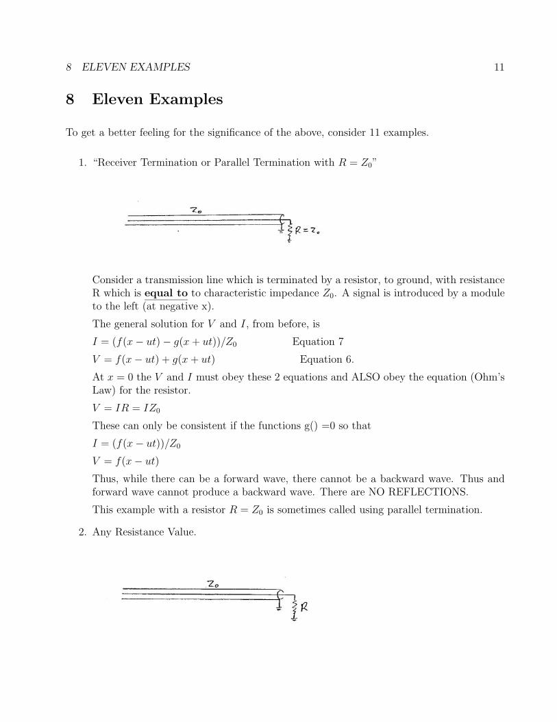
1. “Receiver Termination or Parallel Termination with R = Z0”
Consider a transmission line which is terminated by a resistor, to ground, with resistanceR which is equal to to characteristic impedance Z0. A signal is introduced by a moduleto the left (at negative x).
The general solution for V and I, from before, is
I = (f(x− ut)− g(x+ ut))/Z0 Equation 7
V = f(x− ut) + g(x+ ut) Equation 6.
At x = 0 the V and I must obey these 2 equations and ALSO obey the equation (Ohm’sLaw) for the resistor.
V = IR = IZ0
These can only be consistent if the functions g() =0 so that
I = (f(x− ut))/Z0
V = f(x− ut)Thus, while there can be a forward wave, there cannot be a backward wave. Thus andforward wave cannot produce a backward wave. There are NO REFLECTIONS.
This example with a resistor R = Z0 is sometimes called using parallel termination.
2. Any Resistance Value.
8 ELEVEN EXAMPLES 12
Now consider a similar signal introduced from the left but with a general value of Rinstead of requiring R = Z0.
V = f + g
I = fZ0− g
Z0
If V = IR then
V = f + g = ( fZ0− g
Z0).R
f + g = f RZ0− g R
Z0
f(1− RZ0
) = −g(1 + RZ0
)
g = f.(R−Z0
R+Z0)
Thus the forward wave causes a backward wave. The backward wave is, in general, smallerand we callR = g
f= (R−Z0
R+Z0) the “voltage reflection coefficient”.
checks
• If the cable has Z0 = 50 ohm and the resistor has R = 100 ohm then
R = gf
= 100−50100+50
= 13
• If R = Z0, the Voltage Reflection Coefficient R = gf
= (R−Z0
R+Z0) = 0
2R= 0 as in the
previous example.
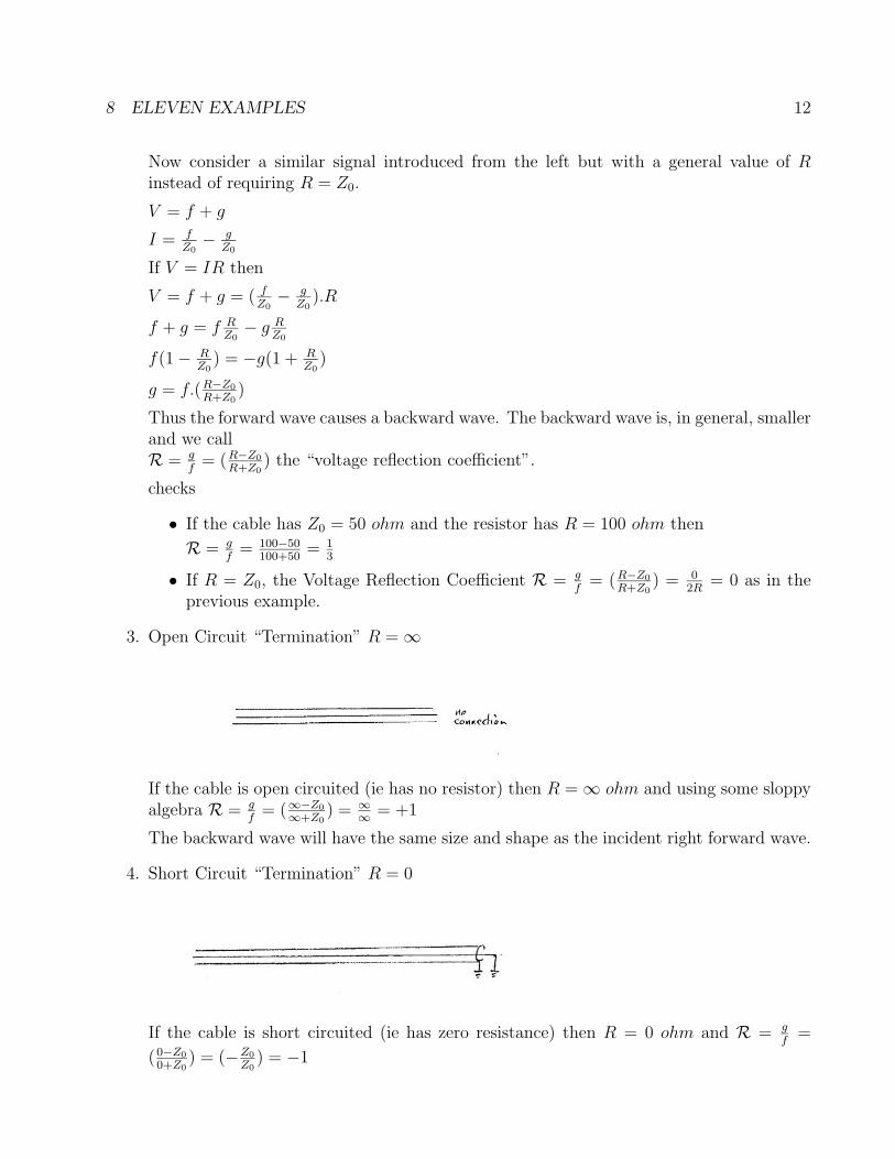
3. Open Circuit “Termination” R =∞
If the cable is open circuited (ie has no resistor) then R =∞ ohm and using some sloppyalgebra R = g
f= (∞−Z0
∞+Z0) = ∞
∞ = +1
The backward wave will have the same size and shape as the incident right forward wave.
4. Short Circuit “Termination” R = 0
If the cable is short circuited (ie has zero resistance) then R = 0 ohm and R = gf
=
(0−Z0
0+Z0) = (−Z0
Z0) = −1
8 ELEVEN EXAMPLES 13
The backward wave will have the same size and shape as the incident right forward wavebut will be inverted.
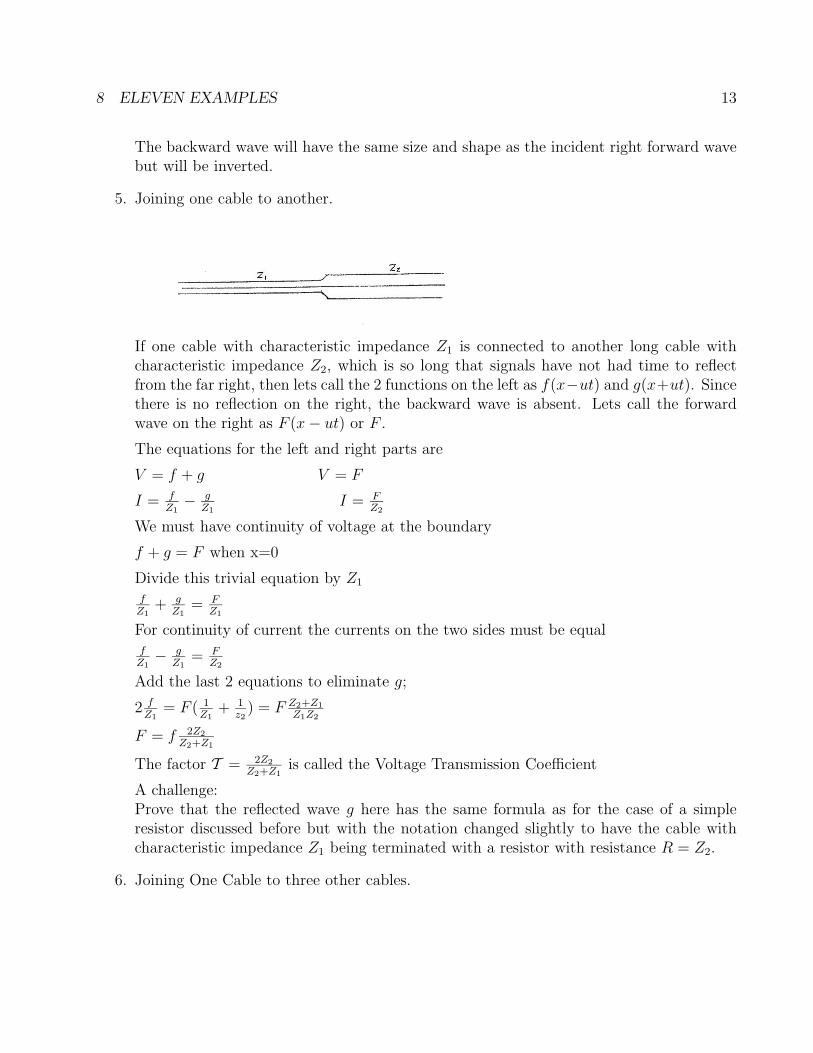
5. Joining one cable to another.
If one cable with characteristic impedance Z1 is connected to another long cable withcharacteristic impedance Z2, which is so long that signals have not had time to reflectfrom the far right, then lets call the 2 functions on the left as f(x−ut) and g(x+ut). Sincethere is no reflection on the right, the backward wave is absent. Lets call the forwardwave on the right as F (x− ut) or F .
The equations for the left and right parts are
V = f + g V = F
I = fZ1− g
Z1I = F
Z2
We must have continuity of voltage at the boundary
f + g = F when x=0
Divide this trivial equation by Z1
fZ1
+ gZ1
= FZ1
For continuity of current the currents on the two sides must be equalfZ1− g
Z1= F
Z2
Add the last 2 equations to eliminate g;
2 fZ1
= F ( 1Z1
+ 1z2
) = F Z2+Z1
Z1Z2
F = f 2Z2
Z2+Z1
The factor T = 2Z2
Z2+Z1is called the Voltage Transmission Coefficient
A challenge:Prove that the reflected wave g here has the same formula as for the case of a simpleresistor discussed before but with the notation changed slightly to have the cable withcharacteristic impedance Z1 being terminated with a resistor with resistance R = Z2.
6. Joining One Cable to three other cables.
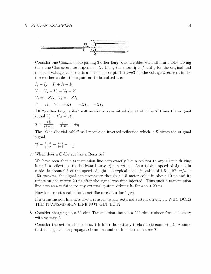
8 ELEVEN EXAMPLES 14
Consider one Coaxial cable joining 3 other long coaxial cables with all four cables havingthe same Characteristic Impedance Z. Using the subscripts f and g for the original andreflected voltages & currents and the subscripts 1, 2 and3 for the voltage & current in thethree other cables, the equations to be solved are:
If − Ig = I1 + I2 + I3
Vf + Vg = V1 = V2 = V3
Vf = +ZIf , Vg = −ZIg,V1 = V2 = V3 = +ZI1 = +ZI2 = +ZI3
All “3 other long cables” will receive a transmitted signal which is T times the originalsignal Vf = f(x− ut).
T =2Z
3
(Z3
+Z)= 2Z
Z+3Z= +1
2
The “One Coaxial cable” will receive an inverted reflection which is R times the originalsignal.
R =Z3−Z
Z3
+Z= 1−3
1+3= −1
2
7. When does a Cable act like a Resistor?
We have seen that a transmission line acts exactly like a resistor to any circuit drivingit until a reflection (the backward wave g) can return. As a typical speed of signals incables is about 0.5 of the speed of light – a typical speed in cable of 1.5 × 10⁸ m/s or150 mm/ns, the signal can propagate though a 1.5 meter cable in about 10 ns and itsreflection can return 20 ns after the signal was first injected. Thus such a transmissionline acts as a resistor, to any external system driving it, for about 20 ns.
How long must a cable be to act like a resistor for 1 µs?
If a transmission line acts like a resistor to any external system driving it, WHY DOESTHE TRANSMISSION LINE NOT GET HOT?
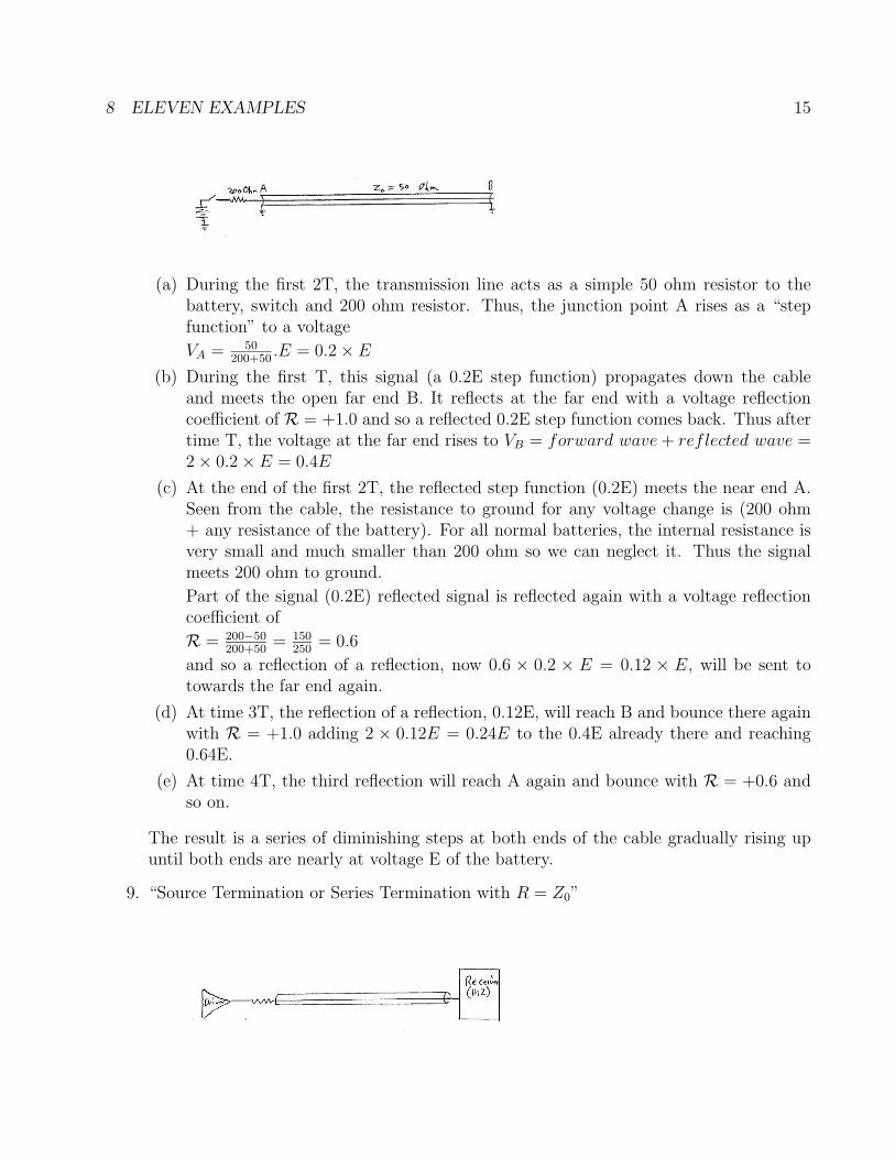
8. Consider charging up a 50 ohm Transmission line via a 200 ohm resistor from a batterywith voltage E.
Consider the action when the switch from the battery is closed (ie connected). Assumethat the signals can propagate from one end to the other in a time T .
8 ELEVEN EXAMPLES 15
(a) During the first 2T, the transmission line acts as a simple 50 ohm resistor to thebattery, switch and 200 ohm resistor. Thus, the junction point A rises as a “stepfunction” to a voltage
VA = 50200+50
.E = 0.2× E(b) During the first T, this signal (a 0.2E step function) propagates down the cable
and meets the open far end B. It reflects at the far end with a voltage reflectioncoefficient of R = +1.0 and so a reflected 0.2E step function comes back. Thus aftertime T, the voltage at the far end rises to VB = forward wave+ reflected wave =2× 0.2× E = 0.4E
(c) At the end of the first 2T, the reflected step function (0.2E) meets the near end A.Seen from the cable, the resistance to ground for any voltage change is (200 ohm+ any resistance of the battery). For all normal batteries, the internal resistance isvery small and much smaller than 200 ohm so we can neglect it. Thus the signalmeets 200 ohm to ground.
Part of the signal (0.2E) reflected signal is reflected again with a voltage reflectioncoefficient of
R = 200−50200+50
= 150250
= 0.6
and so a reflection of a reflection, now 0.6 × 0.2 × E = 0.12 × E, will be sent totowards the far end again.
(d) At time 3T, the reflection of a reflection, 0.12E, will reach B and bounce there againwith R = +1.0 adding 2 × 0.12E = 0.24E to the 0.4E already there and reaching0.64E.
(e) At time 4T, the third reflection will reach A again and bounce with R = +0.6 andso on.
The result is a series of diminishing steps at both ends of the cable gradually rising upuntil both ends are nearly at voltage E of the battery.
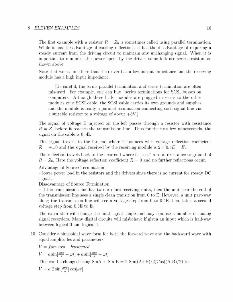
9. “Source Termination or Series Termination with R = Z0”
8 ELEVEN EXAMPLES 16
The first example with a resistor R = Z0 is sometimes called using parallel termination.While it has the advantage of causing reflections, it has the disadvantage of requiring asteady current from the driving circuit to maintain any unchanging signal. When it isimportant to minimize the power spent by the driver, some folk use series resistors asshown above.
Note that we assume here that the driver has a low output impedance and the receivingmodule has a high input impedance.
[Be careful, the terms parallel termination and series termination are oftenmis-used. For example, one can buy “series terminations for SCSI busses oncomputers. Although these little modules are plugged in series to the othermodules on a SCSI cable, the SCSI cable carries its own grounds and suppliesand the module is really a parallel termination connecting each signal line viaa suitable resistor to a voltage of about +3V.]
The signal of voltage E injected on the left passes through a resistor with resistanceR = Z0 before it reaches the transmission line. Thus for the first few nanoseconds, thesignal on the cable is 0.5E.
This signal travels to the far end where it bounces with voltage reflection coefficientR = +1.0 and the signal received by the receiving module is 2× 0.5E = E.
The reflection travels back to the near end where it “sees” a total resistance to ground ofR = Z0. Here the voltage reflection coefficient R = 0 and no further reflections occur.
Advantage of Source Termination– lower power load in the resistors and the drivers since there is no current for steady DCsignals.Disadvantage of Source Termination– if the transmission line has two or more receiving units, then the unit near the end ofthe transmission line sees a single clean transition from 0 to E. However, a unit part-wayalong the transmission line will see a voltage step from 0 to 0.5E then, later, a secondvoltage step from 0.5E to E.
The extra step will change the final signal shape and may confuse a number of analogsignal recorders. Many digital circuits will misbehave if given an input which is half-waybetween logical 0 and logical 1.
10. Consider a sinusoidal wave form for both the forward wave and the backward wave withequal amplitudes and parameters.
V = forward+ backward
V = a sin[2πxλ− ωt] + a sin[2πx
λ+ ωt]
This can be changed using SinA + Sin B = 2 Sin((A+B)/2)Cos((A-B)/2) to
V = a 2 sin[2πxλ
] cos[ωt]
9 CAPACITIVE TERMINATION 17
Note that the dependence upon position x and t has been separated and even though twosignals are involved there appears to be no propagation. Also the signal at any point issimply an alternative voltage.
Signals like these can be caused by simply reflecting a sinusoidal input from an open orvery high impedance at the far end, appear as standing waves. At some positions, theamplitude of the alternating voltage is zero and at other positions the amplitude of thealternating voltage can be 2a.
11. A puzzleRegard the jumper cable you use to start a car with a flat battery from another car as aperfect transmission line with characteristic impedance Z0 = 100 ohm with both batterieshaving an internal resistance of about 1
10ohm. How does the voltage at the flat battery
vary when you connect the jumpers and how is energy transferred to the flat battery?
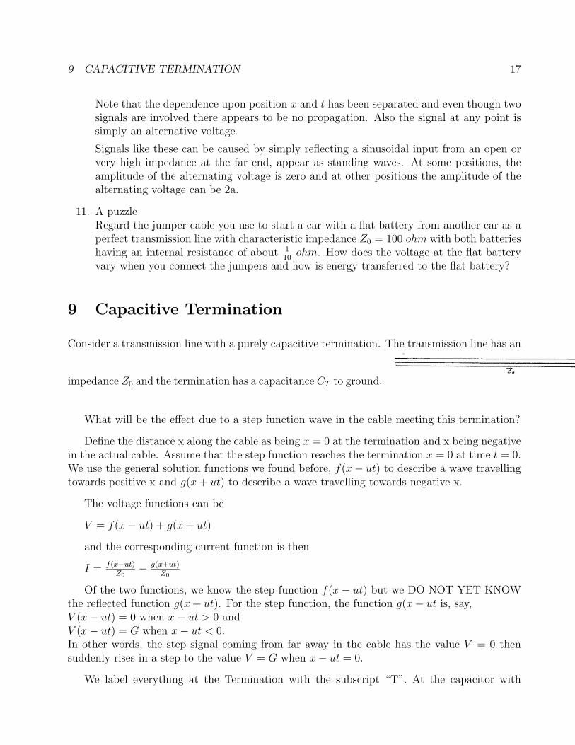
9 Capacitive Termination
Consider a transmission line with a purely capacitive termination. The transmission line has an
impedance Z0 and the termination has a capacitance CT to ground.
What will be the effect due to a step function wave in the cable meeting this termination?
Define the distance x along the cable as being x = 0 at the termination and x being negativein the actual cable. Assume that the step function reaches the termination x = 0 at time t = 0.We use the general solution functions we found before, f(x− ut) to describe a wave travellingtowards positive x and g(x+ ut) to describe a wave travelling towards negative x.
The voltage functions can be
V = f(x− ut) + g(x+ ut)
and the corresponding current function is then
I = f(x−ut)Z0
− g(x+ut)Z0
Of the two functions, we know the step function f(x− ut) but we DO NOT YET KNOWthe reflected function g(x+ ut). For the step function, the function g(x− ut is, say,V (x− ut) = 0 when x− ut > 0 andV (x− ut) = G when x− ut < 0.In other words, the step signal coming from far away in the cable has the value V = 0 thensuddenly rises in a step to the value V = G when x− ut = 0.
We label everything at the Termination with the subscript “T”. At the capacitor with
9 CAPACITIVE TERMINATION 18
capacitance CT , the current combination of the step f(x − ut) travelling towards +x and itsunknown reflection g(x+ut) travelling towards -x will provide a current to charge the capacitor.If VC and IC are the voltage and charging current at the capacitor, then the two equations forthe voltage and current of the two travelling waves are:
VT = f + g
IT = f−gz0
On the capacitor CT , the charge is QT = CTVT and the voltage rises due to the current
dVTdt
= 1Z0CT
(f − g)
dVTdt
= 1Z0CT
(f − (VT − f))
dVTdt
= 1Z0CT
(2f − VT )
After t = 0 at x = 0, f = G and V = VT and so
dVTdt
= − 1Z0CT
(VT − 2G) “differential equation”.
This has a solution for the voltage VT at the termination:
VT − 2G = Ke−t
Z0CT
[Proof. Differentiate the tentative solution and get: VTdt
= − 1Z0C
Ke−t
Z0CT . Then sub-
stitute the differential equation to eliminate Ke−t
Z0CT . This gives VTdt
= − 1Z0CT
(VT −2G) which satisfies the differential equation. ]
Find the value of K. At t = 0,
VT − 2Ge0 = K
0− 2G = K
1. The general solution after t = 0 is
VT − 2G = −2Ge−t
Z0CT
VT = (1− e−t
Z0CT )2G
Since V = f + g and after t = 0, we still have f = G
g = VT −G
g = (1− 2e−t
Z0CT )G
and in the general case with x < 0;
g(x+ ut) = (1− 2e−(x+ut)uZ0CT )G
9 CAPACITIVE TERMINATION 19
Using the signal speed u =√
1LC
and cable impedance Z0 =√
LC
,where L is the inductance per unit length,C is the capacitance per unit length,CT is the terminating capacitance andG is the step of the wave travelling towards the termination,we have uZ0 = L and so
g(x+ ut) = (1− 2e−(x+ut)LCT )G
2. The general solution for g(x+ ut) before t = 0 is g = 0
From the two items above, the reflected waveform is g(x+ ut) where;
1. if x+ ut > 0 then g(x+ ut) = (1− 2e−t
Z0CT )G
2. if x+ ut < 0 then g(x+ ut) = 0
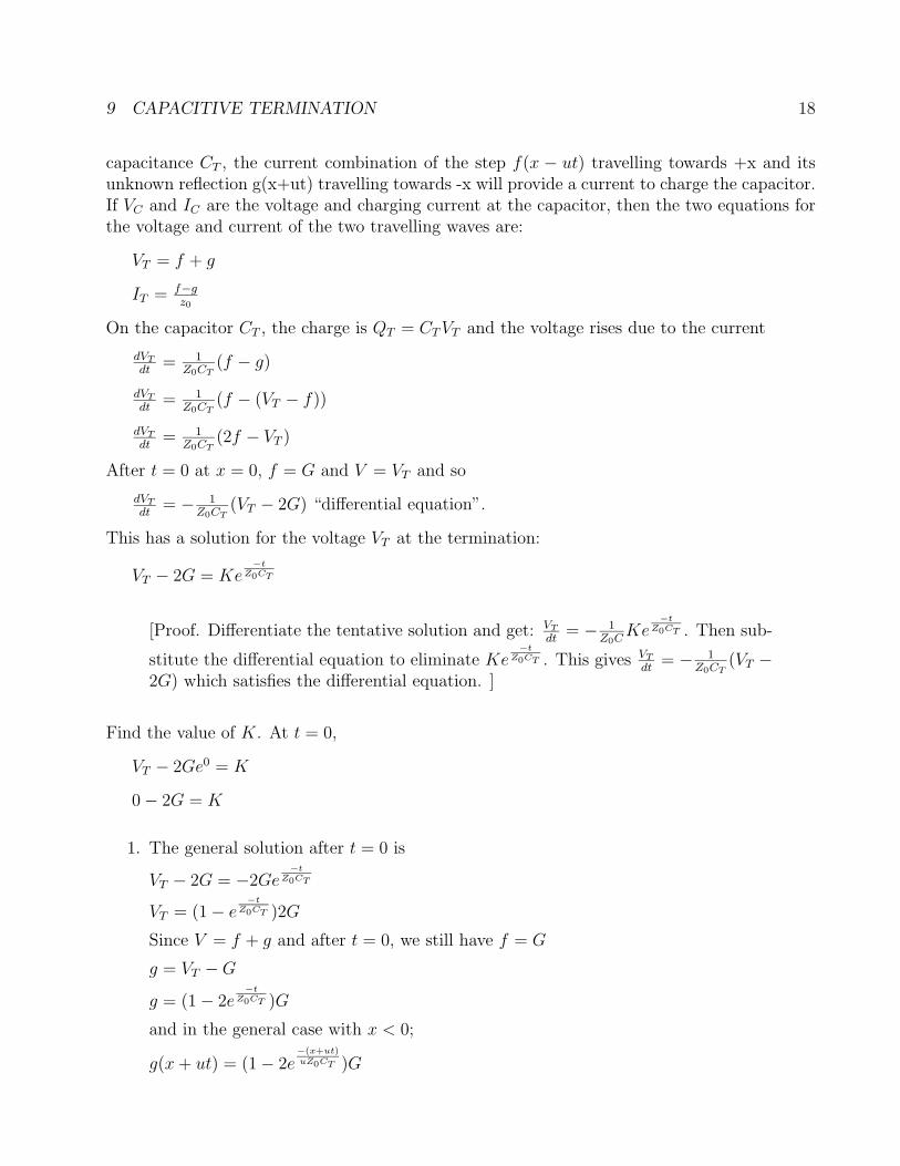
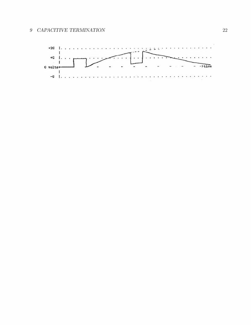
The reflected wave due to a positive step G, starts with a negative step to -G and is followedby an exponential rise to +G. An oscilloscope at any point will see an addition of the initialstep wave f(x− ut) and reflected wave g(x+ ut).
The initial step wave f(x− ut) at an arbitrary x will show the trace on the scope:
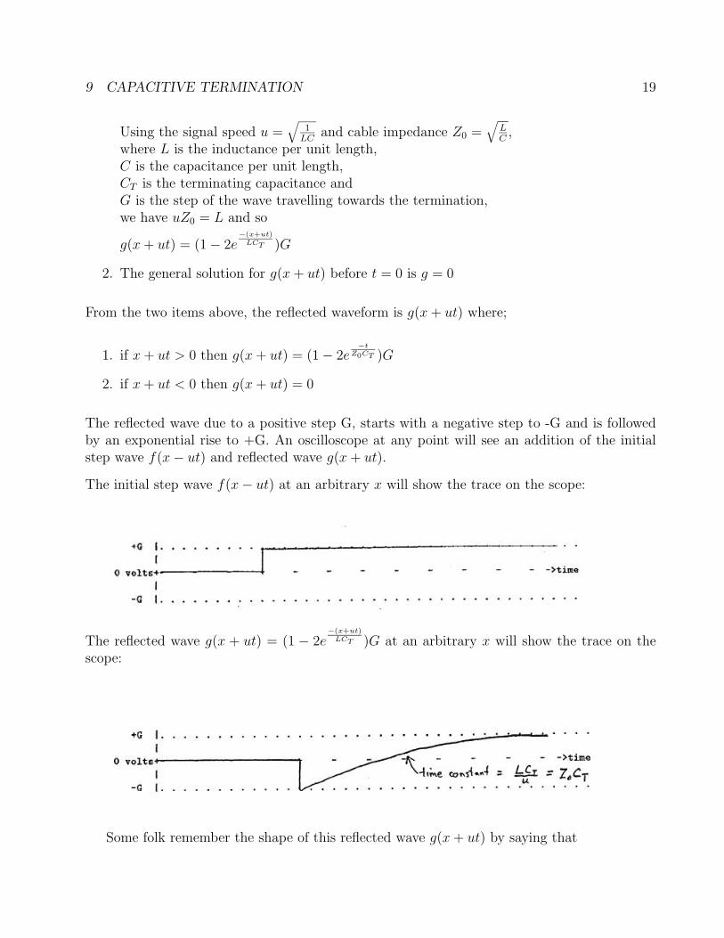
The reflected wave g(x + ut) = (1 − 2e−(x+ut)LCT )G at an arbitrary x will show the trace on the
scope:
Some folk remember the shape of this reflected wave g(x+ ut) by saying that
9 CAPACITIVE TERMINATION 20
1. the leading edge of the step is formed from the high frequencies being in phase and these“see” the capacitor as a short circuit giving a leading negative reflection.
2. the trailing level of the step is formed from the low frequencies being in phase and these“see” the capacitor as an open circuit giving a trailing positive reflection.
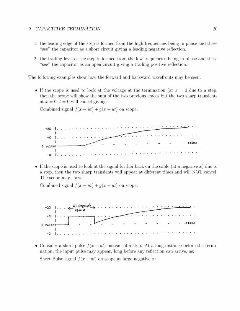
The following examples show how the forward and backward wavefronts may be seen.
• If the scope is used to look at the voltage at the termination (at x = 0 due to a step,then the scope will show the sum of the two previous traces but the two sharp transientsat x = 0, t = 0 will cancel giving:
Combined signal f(x− ut) + g(x+ ut) on scope:
• If the scope is used to look at the signal further back on the cable (at a negative x) due toa step, then the two sharp transients will appear at different times and will NOT cancel.The scope may show:
Combined signal f(x− ut) + g(x+ ut) on scope:
• Consider a short pulse f(x − ut) instead of a step. At a long distance before the termi-nation, the input pulse may appear, long before any reflection can arrive, as:
Short Pulse signal f(x− ut) on scope at large negative x:
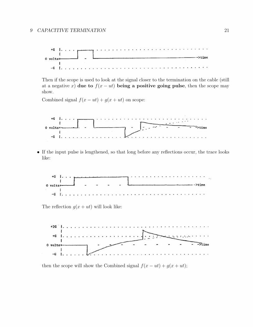
9 CAPACITIVE TERMINATION 21
Then if the scope is used to look at the signal closer to the termination on the cable (stillat a negative x) due to f(x− ut) being a positive going pulse, then the scope mayshow.
Combined signal f(x− ut) + g(x+ ut) on scope:
• If the input pulse is lengthened, so that long before any reflections occur, the trace lookslike:
The reflection g(x+ ut) will look like:
then the scope will show the Combined signal f(x− ut) + g(x+ ut);
9 CAPACITIVE TERMINATION 22
10 TYPES OF TRANSMISSION LINES 23
10 Types of Transmission Lines
(Brief Notes Follow)
Any pair of parallel conductors which have a cross and shape which are constant (indepen-dent of distance) and are far from other conductors
or any pair of parallel conductors which have a cross and shape which do not change rapidlyand retain the same ratios of dimensions (independent of distance along the pair) and are farfrom other conductors.
If one conductor does not fully enclose the other conductor (eg twisted pair), then someof the EM field will gradually radiate away and the signal will show a steady attenuation andexponential decay which is frequency dependent.
Examples:
1. An example could be a single cylindrical conductor (wire) above a conducting plane withthe wire diameter changing slowly and the distance between the wire center and theconducting plane being kept proportional to the wire diameter.
2. Twisted pair wire – often with Z0 ≈ 120 ohm
3. 60 Hertz High Voltage Power Lines across the country. Strictly speaking these are usuallya combination of 6 interacting transmission lines with the phase at 60 degree intervals.
The speed of power transmission is very close to that of light uair = 1√µairεair
≈ V elocity of light.
4. Ethernet coaxial cables all around Sterling Hall and Chamberlin Hall. Both haveZ0 = 50± 1 ohm. There are two types; yellow “thick ethernet” cables have large conduc-tors to have minimum resistance attenuation, black RG58/U cables “thin ethernet” arethinner for least cost.
5. Electrical Transmission Lines are not Waveguides or Light Guides.
6. The 60 Hertz power lines across the country are imperfect. There is some leakage orradiation of the 60 Hertz field since the conductors are open. There is a financial incentiveto arrange the phases of the 6 conductors so that the minimum radiation occurs.There is other attenuation due to slight breakdown on the insulators and corona in theair. On the average about the USA, there is about a 10% power loss??)
7. Besides the loss of power by radiation, there is another problem of open conductors —unwanted coupling to other circuits. This is not a problem at the lower frequencies butcan be awful at high frequencies.

11 IMPERFECTIONS OF TRANSMISSION LINES 24
11 Imperfections of Transmission Lines
1. Radiation from open conductors mentioned aboveUse Coaxial transmission lines if these are practical.
2. Skin Effect lossesThese are due to the actual currents being confined by the skin effect to the surface layersof the conductors. (EM Theory)
Most current occurs within a distance “skin thickness” δ whereδ =
√2
ωµσwhere ω = 2π × frequency.
Consider 3 examples
• For copper, which is pure and has been annealed, at 20 C,conductivity σCu = 1
Resistivity= 5.80× 10⁷ mho/m
µ = µair = 4π107 H/m
ω = 2π × frequency giving
δ =√
2ωµσ
= 0.0661 meter.hertz12√
Freqency
Starting at the surface of the conductor, the current density J drops to 1e
at depthδ and a total of 1% of the total current exists at depth beyond 5δ.
For example, in thick copper lines carrying power at 60 Hertz,
δ60 Hertz, Cu = 0.0661√60
= 0.0085 meter = 8.5 mm!!!
Thus at 60 Hertz, only the outer centimeter of the 8 or 10 cm diameter lines carrymost of the current.
• The thick aluminum power lines used for high voltage distribution have a conduc-tivity of σAl = 3.77× 10⁷ mho/meter.
δ60 Hertz, Al =√
2ωµσAl
= 0.0105 meter = 10.5 mm!!
[Why is aluminum, rather than copper, used for our National power sys-tem? Calculate the resistance of a 10,000 km line or rod for both materialsassuming that the effective cross sectional area used in each line is 2πrδ andthe radius is r = 100 mm. Also calculate the cost of each line or rod using;Aluminum conductivity σAl = 3.77 × 10⁷ mho/m, density= 2708 kg/m3
cost/kg= 7.70 $/kg.Copper conductivity σCu = 5.80×10⁷ mho/m, density= 2567 kg/m3 cost/kg=15.40 $/kg.]
Do the centers of the heavy power lines have much use?
• For copper lines at frequencies near 60 MHz, δ = 0.0661 meter.hertz12√
60×106 hertz= 8.5 microns!!!
Since the skin depth is frequency dependent, the effect is to attenuate the highfrequencies of the signal more rapidly than the low frequencies of the signal. Thusthe signal CHANGES ITS SHAPE during the propagation due to the skin effect.
11 IMPERFECTIONS OF TRANSMISSION LINES 25
11.1 “Remedies” for Signal Loss
On copper at high frequencies, the skin depth (8.5 microns at 60 MHz) can be serious.
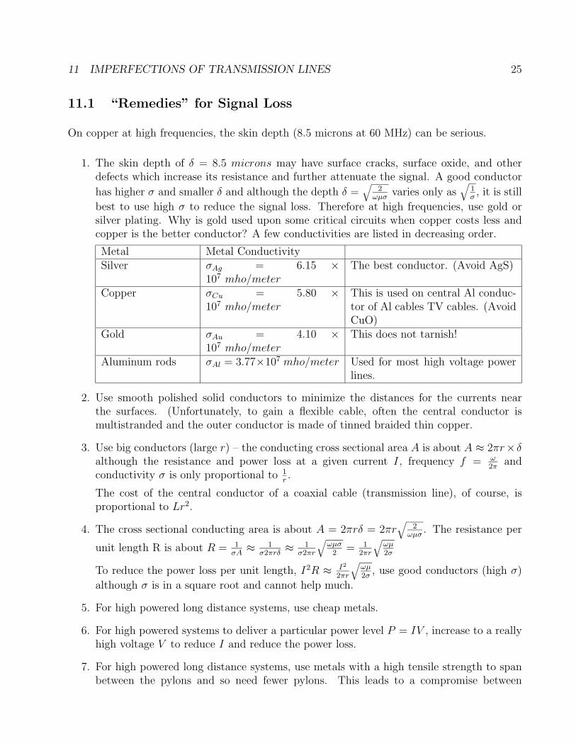
1. The skin depth of δ = 8.5 microns may have surface cracks, surface oxide, and otherdefects which increase its resistance and further attenuate the signal. A good conductor
has higher σ and smaller δ and although the depth δ =√
2ωµσ
varies only as√
1σ, it is still
best to use high σ to reduce the signal loss. Therefore at high frequencies, use gold orsilver plating. Why is gold used upon some critical circuits when copper costs less andcopper is the better conductor? A few conductivities are listed in decreasing order.
Metal Metal ConductivitySilver σAg = 6.15 ×
107 mho/meterThe best conductor. (Avoid AgS)
Copper σCu = 5.80 ×10⁷ mho/meter
This is used on central Al conduc-tor of Al cables TV cables. (AvoidCuO)
Gold σAu = 4.10 ×10⁷ mho/meter
This does not tarnish!
Aluminum rods σAl = 3.77×10⁷ mho/meter Used for most high voltage powerlines.
2. Use smooth polished solid conductors to minimize the distances for the currents nearthe surfaces. (Unfortunately, to gain a flexible cable, often the central conductor ismultistranded and the outer conductor is made of tinned braided thin copper.
3. Use big conductors (large r) – the conducting cross sectional area A is about A ≈ 2πr× δalthough the resistance and power loss at a given current I, frequency f = ω
2πand
conductivity σ is only proportional to 1r.
The cost of the central conductor of a coaxial cable (transmission line), of course, isproportional to Lr2.
4. The cross sectional conducting area is about A = 2πrδ = 2πr√
2ωµσ
. The resistance per
unit length R is about R = 1σA≈ 1
σ2πrδ≈ 1
σ2πr
√ωµσ
2= 1
2πr
√ωµ2σ
To reduce the power loss per unit length, I2R ≈ I2
2πr
√ωµ2σ
, use good conductors (high σ)
although σ is in a square root and cannot help much.
5. For high powered long distance systems, use cheap metals.
6. For high powered systems to deliver a particular power level P = IV , increase to a reallyhigh voltage V to reduce I and reduce the power loss.
7. For high powered long distance systems, use metals with a high tensile strength to spanbetween the pylons and so need fewer pylons. This leads to a compromise between
12 EQUATIONS FOR A “LOSSY” TRANSMISSION LINE 26
conductivity σ and tensile strength. If practical, in each wire or rod carrying current, usea high tensile inner wire surrounded by high conductivity but weaker outer wires. Thenworry about corrosion!
8. Beware of damaged coaxial cable causing unwanted reflections and reductions in theforward signal. Crushed coax has a lower Z0 and the lumpy dielectric can change Z0 –both cause reflections.
9. Speeds in some cables can be SLOW! Even if no magnetic materials are used (ie µ = µ0),then
u = c√εr
If necessary, use a foam dielectric with εr ≈ 1 giving u close to the speed of light.
10. Minimize the resistance of the outer conductor.
11. Minimize electrical breakdown.
12. Choose your connectors carefully. Even the coaxial connectors often have a Z0 which isdifferent from that of the cables and cause a pair of reflections which have the same shapeand opposite sign but do not cancel because they occur at slightly different times.
Noncoaxial connectors often have short links with relatively high characteristic impedanceand these impedance transitions can cause a number of upright and inverted reflectionswhich are close together but not cancelling.
13. For small signals being sent over long distance systems, use optical fibers!
12 Equations for a “Lossy” Transmission Line
In section 2 before, on page 2, we began to consider “Lossless” transmission lines. However,sometimes, we must use transmission lines with the series resistance/unit length being non-zero and the insulation being non-perfect with a parallel conductance of G being non-zero. Auseful simple reference is “Theory and Problems of Transmission Lines” by Robert A. Chipman(Schaum Outline Series 1968). We will continue to use x for the distance along the transmissionline whereas Chipman uses z for this. Our x will avoid confusion between the distance and thecharacteristic impedance Z.
Consider a transmission line with distributed resistance R ohm/unit length and parallelconductance G mho/unit length.
12 EQUATIONS FOR A “LOSSY” TRANSMISSION LINE 27
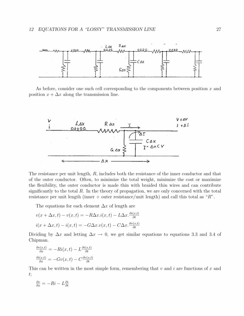
As before, consider one such cell corresponding to the components between position x andposition x+ ∆x along the transmission line.
The resistance per unit length, R, includes both the resistance of the inner conductor and thatof the outer conductor. Often, to minimize the total weight, minimize the cost or maximizethe flexibility, the outer conductor is made thin with braided thin wires and can contributesignificantly to the total R. In the theory of propagation, we are only concerned with the totalresistance per unit length (inner + outer resistance/unit length) and call this total as “R”.
The equations for each element ∆x of length are
v(x+ ∆x, t)− v(x, t) = −R∆x.i(x, t)− L∆x.∂i(x,t)∂t
i(x+ ∆x, t)− i(x, t) = −G∆x.v(x, t)− C∆x.∂v(x,t)∂t
Dividing by ∆x and letting ∆x → 0, we get similar equations to equations 3.3 and 3.4 ofChipman.
∂v(x,t)∂x
= −Ri(x, t)− L∂i(x,t)∂t
∂i(x,t)∂x
= −Gv(x, t)− C ∂v(x,t)∂t
This can be written in the most simple form, remembering that v and i are functions of x andt;
∂v∂x
= −Ri− L∂i∂t
12 EQUATIONS FOR A “LOSSY” TRANSMISSION LINE 28
∂i∂x
= −Gv − C ∂v∂t
These equations are similar, of course, to the equations 2 and 1 which we obtained upon page3 but now include the non-zero R and G.
As before, we can substitute for i in one equation from the other to obtain a differentialequation in v. Similarly we can obtain a differential equation for i.
∂2v∂x2 = LC.∂
2v∂t2
+ (LG+RC).∂v∂t
+RGv
∂2i∂x2 = LC.∂
2i∂t2
+ (LG+RC).∂i∂t
+RGi
Notes
1. These equations do not have the simple form and simple solution of the equations for a“lossless” line.
2. Although we have assumed that the L, C, R and G are constants, at high frequencies,these can be frequency dependent. For example, they may be influenced by the skin effectwhich is frequency dependent.
Never the less, if we consider just one Fourier component of a signal, we can obtain anunderstanding, then by combining the Fourier components of any particular signal, wecan understand how a particular signal propagates.
3. Although the equations above for v and i are identical, they will usually have differentboundary conditions and so will have different solutions.
We can replace v(x, t) by Re{V (x)ejωt} and i(x, t) by Re{I(x)ejωt}dV (x)dx
= −(R + jωL)I(x)
dI(x)dx
= −(G+ jωC)V (x)
From these we get two second order differential equations similar to Equations 3.15 and 3.16of Whitman.
d2Vdx2 − (R + jωL)(G+ jωC)V = 0
d2Idx2 − (R + jωL)(G+ jωC)I = 0
We define γ where γ2 = (R + jωL)(G+ jωC).
d2Vdx2 − γ2V = 0
d2Idx2 − γ2I = 0
The solutions for these are voltages and currents with an angular frequency ω.
V (x) = V1e−γx + V2e
+γx
12 EQUATIONS FOR A “LOSSY” TRANSMISSION LINE 29
I(x) = I1e−γx + I2e
+γx
where V1, V2, I1 and I2 are arbitrary constants andwhere γ2 = (R+ jωL)(G+ jωC). Define α and β as the real and imaginary parts of γ so that
γ = α + jβ =√
(R + jωL)(G+ jωC)
Then the solution for V is
V (x, t) = [ejθ1 .V1e−(αx+jβx) + ejθ2 .V2e
+(αx+jβx)]
V (x, t) = [ejθ1 .V1e−αxe−jβx + ejθ2 .V2e
+αxe+jβx]
Using v(x.t) = Re{V.ejωt}, this becomes
v(x, t) = Re{ejωt.[ejθ1 .V1e−αxe−jβx + ejθ2 .V2e
+αxe+jβx]}
v(x, t) = V1e−αxRe{ej(ωt−βx+θ1)}+ V2e
+αxRe{ej(ωt+βx+θ2)}
corresponding to a forward (x increasing) wave + a backward (x decreasing) wave. The partsof this equation can be identified.
• V1 is an arbitrary amplitude for a signal propagating in the +x direction.
• e−αx is a real coefficient diminishing in the forward or +x direction and describing theattenuation of the signal as its moves in that direction.
• (ωt− βx) is a term describing a wave propagating in the + x direction with phase speedu = +ω
βsince if t is increased by ∆t, then the value is unchanged if the x is increased by
∆x = +ωβ
∆t. The group speed is = +dωdβ
.
• θ1 is an arbitrary phase angle
• ej(ωt−βx+θ1) is a sinusoidal wave of angular frequency ω propagating in the + x directionwith phase speed = +ω
βand group speed = +dω
dβ.
• V2 is an arbitrary amplitude for a signal propagating in the -x direction.
• eαx is a real coefficient diminishing in the backward or -x direction and describing theattenuation of the signal as its moves in that direction.
• (ωt + βx) is a term describing a wave propagating in the - x direction with phase speedu = −ω
βsince if t is increased by ∆t, then the value is unchanged if the x is decreased by
∆x = ωβ
∆t. The group speed is = −dωdβ
.
• θ2 is an arbitrary phase angle
• ej(ωt+βx+θ2) is a sinusoidal wave of angular frequency ω propagating in the - x directionwith phase speed u = −ω
βand group speed = −dω
dβ.
13 LOSSY LINE WITH NO REFLECTIONS 30
• v(x.t) is the instantaneous voltage at position x and time t.
13 Lossy Line with No Reflections
If only the forward wave exists, the equations become;
V = V1e−αze−jβz
I = I1e−αze−jβz
14 Attenuation if line is slightly lossy
α and β may be written
α + jβ =√
(R + jωL).(G+ jωC)
α + jβ = jω√LC.[( R
jωL+ 1)
12 .( G
jωC+ 1)
12 ]
Now use a Taylor expansion of each ()12 as power series of R
jωLand G
jωC
α + jβ = jω√LC.[(...+ (
12
( 12−1)
1×2).( R
jωL)2 + 1
2. RjωL
+ 1) . (...+ (12
( 12−1)
1×2).( G
jωC)2 + 1
2. GjωC
+ 1)]
α + jβ = jω√LC.[(...− 1
8.( RjωL
)2 + 12. RjωL
+ 1).(...+ 18.( GjωC
)2 + 12. GjωC
+ 1)]
L and C are usually log functions of ratios of cable radii or other cable dimensions and so cannotbe very high or very small. However, if R and G are small but non-zero OR the frequency f = ω
2π
is very high, so that RjωL
<< 1 and GjωC
<< 1, then these two Taylor series can be simplified by
neglecting the higher powers of RjωL
and GjωC
.
α + jβ = jω√LC.[( R
j2ωL+ 1).( G
j2ωC+ 1)]
Equating the real parts;
α = ω√LC.[ R
2ωL+ G
2ωC]
α =√LC2.[RL
+ GC
]
Equating the imaginary parts;
jβ = jω√LC.[1 + ( R
2jωLG
2jωC)]
β = ω√LC.[1− RG
4ω2LC]
15 CHARACTERISTIC IMPEDANCE OF A LOSSY TRANSMISSION LINE 31
β ≈ ω√LC (neglecting the product of R
jωLand G
jωC).
From β, we can obtain the phase speed u = ωβ
= 1√LC
, and group speed = dωdβ
= 1√LC
.
[Make a check of these equations for the lossless transmission line. If R = G = 0,then
α =√LC2.[0 + 0] = 0 and so, as expected, there is no attenuation of either the
forward wave or backward wave.β = ω
√LC.[1− 0] = ω
√LC
The full equation can be written for the lossless case.v(x, t) = V1e
−αxRe{ej(ωt−βx+θ1)}+ V2e+αxRe{ej(ωt+βx+θ2)}
becomesv(x, t) = V1Re{ej(ωt−βx+θ1)}+ V2Re{ej(ωt+βx+θ2)}]
15 Characteristic Impedance of a Lossy Transmission
Line
We get VI
=√
R+jωLG+jωC
This is the characteristic impedance and can be split into real and imaginary parts
Z0 =√
R+jωLG+jωC
Z0 = R0 + jX0
If the transmission line is only slightly lossy, then R and G are small and, for most purposes,we ignore X0.
16 Heavyside Distortionless Lines
If RL
= GC
, then it can be shown that the speed of propagation is the same for all angularfrequencies ω and the shape of the signal with respect to position X, remains constant althoughit gradually gets smaller with the attenuation.
Unfortunately, this idea has little practical use because the R, L, G and C are sufficientlyfrequency dependent for the above theory to be insufficient.
17 THREE EXAMPLES 32
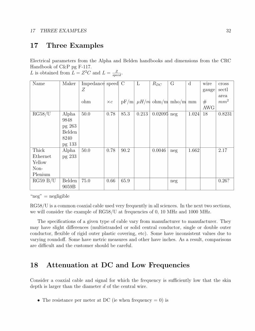
17 Three Examples
Electrical parameters from the Alpha and Belden handbooks and dimensions from the CRCHandbook of C&P pg F-117.L is obtained from L = Z2C and L = Z
speed.
Name Maker ImpedanceZ
speed C L RDC G d wiregauge
crosssectlarea
ohm ×c pF/m µH/m ohm/m mho/m mm #AWG
mm2
RG58/U Alpha9848pg 263Belden8240pg 133
50.0 0.78 85.3 0.213 0.02095 neg 1.024 18 0.8231
ThickEthernetYellowNon-Plenium
Alphapg 233
50.0 0.78 90.2 0.0046 neg 1.662 2.17
RG59 B/U Belden9059B
75.0 0.66 65.9 neg 0.26?
“neg” = negligible
RG58/U is a common coaxial cable used very frequently in all sciences. In the next two sections,we will consider the example of RG58/U at frequencies of 0, 10 MHz and 1000 MHz.
The specifications of a given type of cable vary from manufacturer to manufacturer. Theymay have slight differences (multistranded or solid central conductor, single or double outerconductor, flexible of rigid outer plastic covering, etc). Some have inconsistent values due tovarying roundoff. Some have metric measures and other have inches. As a result, comparisonsare difficult and the customer should be careful.
18 Attenuation at DC and Low Frequencies
Consider a coaxial cable and signal for which the frequency is sufficiently low that the skindepth is larger than the diameter d of the central wire.
• The resistance per meter at DC (ie when frequency = 0) is
18 ATTENUATION AT DC AND LOW FREQUENCIES 33
RDC = 1σ×0.8231 mm2 = 1
5.80×10⁷ mho/m×0.8231×10−6 m2 = 0.209×10⁻¹ ohm/m = 0.0209 ohm/m
This agrees with the CRC handbook of C&P pg F-117 of R=20.95 ohm/km for annealedcopper at a temperature of 20 C.
• The inductance per unit length is L = Z2C = 502 × 85.3× 10−12 H/m
L = 2500× 85.3× 10−12 H/m = 0.213× 10⁻⁶ Henry/meter
• The signal speed is 0.78× c and so u =√
1LC
= 0.78× 3× 108m/s
• The impedance Z is approximately√
LC
= 50 ohm
• The leakage as in most modern cables, is negligible, so set the leakage conductance G = 0.
We can use the speed, the impedance and G = 0 to obtain the attenuation. The attenuationfactor α is then
α =√LC2.[RL
+ GC
]
α =√LC2.[RL
]
Substitute Z =√
LC
α = R2Z
(Chipman pgs 49, 55 & 57)
For RG58/U with no skin effect (ie at DC or low frequencies);
α = 0.020952×50
/meter = 0.2095× 10⁻³ /meter
From α for any cable, we can calculate the number of db loss of that cable over a length x by
db loss = 10× log10( PowerinputPowerat 1 km
)
db loss = 10× log10( VinputVat 1 km
)2
db loss = 20× log10( VinputVat 1 km
)
db loss = 20× log10(eαx)
db loss = 20× loge(eαx)loge10
db loss = 20× αx2.3026
This is often stated simply as
db loss = 8.6858 αx
The attenuation of the voltage signal, due to only the central conductor, on RG58/U over adistance of x = 1 km = 1000 m is;
19 ATTENUATION AT HIGHER FREQUENCIES 34
db loss = 20× 0.2095×10−3 /m×1000 m2.3026
db
db loss = 1.820 db for the 1 km length at zero and low frequencies.
19 Attenuation at Higher Frequencies
19.1 Skin Effect Loss
The loss rate calculated above is for low frequencies in which all of the central conductorconducts the signal. At the higher frequencies, the skin effect reduces the cross section of thecopper which conducts and so the attenuation is increased.
α =√LC2.[RL
]
α = 1
2√
LC
R
α = R2Z
(See Chipman pgs 49 & 85.)
Since for all frequencies above some lower limit, the skin effect restricts the current toapproximately the skin depth of the copper
δ =√
2ωµσ
= 0.0661 meter.hertz12√
Freqency,
we can estimate the approximate resistance/meter at these high frequencies.
For copper lines at frequencies near 10 MHz, δ = 0.0661 meter.hertz12√
10×106 hertz= 20.9 microns. If the di-
ameter of the central conductor is d then, for most cables and frequencies above 1 MHz, δ << d.With this assumption then the conducting region is equivalent to that of a thin shell with a depth of δ.This relation can be proved and is called the “Skin Effect Theorem”. (See Chipman pgs 78& 85.) From this, we can estimate the effective resistance/unit length Rf , at a particularfrequency f . Since the periphery is πd, the cross section of (πd× δ).
Rf ≈ 1σ×(conduction cross sectional area)
Rf ≈ 1σ×(πd×δ)
Rf ≈ 1
σ×(πd×√
2ωµσ
)
Rf ≈ 1πd.√
ωµ2σ
Note that, at the higher frequencies, Rf ∝√ω ∝√f
We estimate the attenuation due to only the central conductor of RG58/U at 10 MHz and1.0 GHz. We do not have enough data to estimate the attenuation due to the outer conductor.
19 ATTENUATION AT HIGHER FREQUENCIES 35
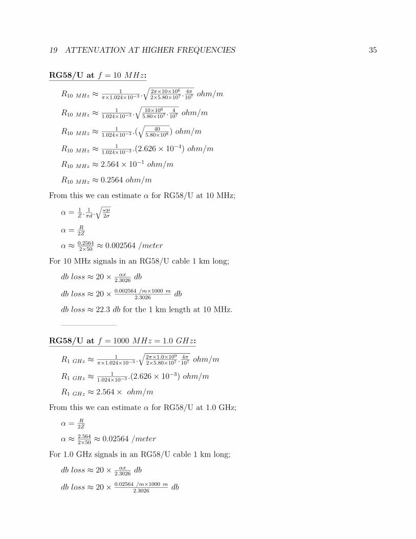
RG58/U at f = 10 MHz:
R10 MHz ≈ 1π×1.024×10−3 .
√2π×10×106
2×5.80×107 .4π107 ohm/m
R10 MHz ≈ 11.024×10⁻³ .
√10×106
5.80×10⁷ .4
107 ohm/m
R10 MHz ≈ 11.024×10⁻³ .(
√40
5.80×10⁸ ) ohm/m
R10 MHz ≈ 11.024×10⁻³ .(2.626× 10⁻⁴) ohm/m
R10 MHz ≈ 2.564× 10⁻¹ ohm/m
R10 MHz ≈ 0.2564 ohm/m
From this we can estimate α for RG58/U at 10 MHz;
α = 1Z. 1πd.√
ωµ2σ
α = R2Z
α ≈ 0.25642×50
≈ 0.002564 /meter
For 10 MHz signals in an RG58/U cable 1 km long;
db loss ≈ 20× αx2.3026
db
db loss ≈ 20× 0.002564 /m×1000 m2.3026
db
db loss ≈ 22.3 db for the 1 km length at 10 MHz.
———————
RG58/U at f = 1000 MHz = 1.0 GHz:
R1 GHz ≈ 1π×1.024×10−3 .
√2π×1.0×109
2×5.80×107 .4π107 ohm/m
R1 GHz ≈ 11.024×10⁻³ .(2.626× 10⁻³) ohm/m
R1 GHz ≈ 2.564× ohm/m
From this we can estimate α for RG58/U at 1.0 GHz;
α = R2Z
α ≈ 2.5642×50≈ 0.02564 /meter
For 1.0 GHz signals in an RG58/U cable 1 km long;
db loss ≈ 20× αx2.3026
db
db loss ≈ 20× 0.02564 /m×1000 m2.3026
db
19 ATTENUATION AT HIGHER FREQUENCIES 36
db loss ≈ 223 db for the 1 km length at 1.0 GHz.
19.2 Dielectric Loss
This attenuation is due to the dielectric absorbing energy as it is polarized in each direction.This loss is usually small but becomes more significant at the higher frequencies.
The effect is that our conductance/unit length becomes non-zero at the higher frequencies.The difference of the phase of the current ∆I between the central conductor and the outerconductor and the phase of the voltage changes from being π
2to π
2− ε and data sheets can
give a loss factor of “Tanε” to give the relation. Unfortunately, we don’t have convenient datasheets for the dielectric of RG58/U.
The usual circuit boards made from epoxy-glass have a significant attenuation due to thedielectric loss while polyethylene has a modest loss.
19.3 Radiation Loss
If the conductors form a tight electromagnetic system with the outer conductor having a thick-ness greater than about 5δ (5 times the skin depth) then external EM fields will be small andthe radiation loss is negligible.
If the outer conductor is a loose braid, the the external EM fields will cause radiation awayfrom the cable and will cause attenuation.
If the transmission line has two open conductors with neither shielding the other, then theexternal fields are minimized by twisting the two conductors (forming a “twisted pair” line).However, even if the pitch of the twist is much smaller than the predominant wavelength of theelectrical signal, some radiation occurs and the signal is attenuated. For this reason, be carefulwhen using twisted pair lines.
[In addition such twisted pair lines can easy receive electrical noise from other circuits whichhave high current or voltage transients.]
19.4 Actual Attenuation in Cables
We can compare the results of these approximate calculations with actual attenuation mea-surements.From the Alpha handbook,
• for RG58/U (pg 273) the loss at the relatively low frequency of 10 MHz of RG58/U is 1.2db/100 ft = 3.94 db/100 meters= 39.4 db/km.
19 ATTENUATION AT HIGHER FREQUENCIES 37
The loss at the relatively high frequency of 1000 MHz is 18.0 db/100 ft = 59 db/100meters = 590 db/km.
• for Thick Ethernet (pg 233) the loss at 10 MHz is 20 db/km.
Obviously, the estimate of the loss due to only the skin effect of the central conductor isabout half of the db of the actual loss. Probably the remaining loss is due to the imperfectouter conductor and to the dielectric loss.(?)
• The central or inner conductor has a smaller periphery but usually has a smooth surfaceand high conducting metal.
• The outer conductor has a smaller periphery but is usually rough (made of braided wiresfor flexibility) with only tinned surfaces and imperfect contacts. The majority of the cablecost is due to the outer metal and so manufacturers may skimp a little on the conductivityof the outer conductor.