Transmission Corridor between Romania-Moldova-Ukraine

UDREA OANA.*, GHEORGHE LAZAROIU. **

* CNTEE Transelectrica SA, Bucharest, ** University “Politehnica” Bucharest

* oana.udrea@gmail.com, ** glazaroiu@yahoo.com

Abstract – Constructed in 1986, the 750 kV line

connecting the Ukrainian and Romanian transmission

networks went out of service in the mid-1990s due to

damage to the lines. Although the Romanian TSO

(Transelectrica) and the Ukrainian TSO (Ukrenergo) carry

plans to restore the line, each has experienced significant

development of their transmission networks since the line

went out of service. This article identifies the optimal

configuration of the corridor to serve the transmission

requirements of the system operators in Romania, Ukraine

and Moldova. Currently the transmission corridor, which

had consisted of a 750kV AC Over Head Line (OHL), is not

in operation and is in a state that cannot be easily repaired.

The OHL has been damaged so that it could be considered

as “non-existent” for each party. The investment scenarios

themselves are comprised two voltage levels considered for

the corridor: 400 kV and 750 KV. In turn, these voltages

can be analyzed in terms of synchronous AC or

asynchronous DC connection via a back-to-back station that

may be located in either Moldova or Romania.

Keywords: asynchronous, back-to-back, IPS/UPS, RUM

I. INTRODUCTION

Currently the Romanian – Moldovan – Ukrainian (RUM)

transmission corridor, which had consisted of a 750kV AC

Over Head Line (OHL), is not in operation and is in a state that

cannot be easily repaired. The OHL has been damaged so that it

could be considered as “non-existent” for each RUM party. The

existing route of the old 750 kV transmission line is depicted in

Fig.1.

Fig. 1. The route of the old 750 kV transmission line

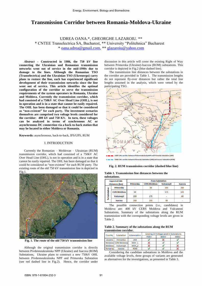
Although the original transmission corridor is directly

between Pivdennoukrainska NPP (Ukraine) and Isaccea (ROM)

Substations, Ukraine plans to construct a new 750kV OHL

between Pivdennoukrainska NPP and Primorska Substation

(see red dashed line in Fig.2). Hence, the corridor under

discussion in this article will cover the existing Right of Way

between Primorska (Ukraine)-Isaccea (ROM) substations. This

corridor is depicted in Fig.2 (blue dashed line).

The transmission line distances between the substations in

the corridor are provided in Table 1. The transmission lengths

do not represent fly-over distances but rather the total line

lengths assumed in the analysis, which were vetted by the

participating TSO.

Fig. 2. RUM transmission corridor (dashed blue line)

Table 1. Transmission line distances between the

substations.

The possible connection points (i.e., candidates) in

Moldova are: 400 kV CERS Moldova and Vulcanesti

Substations. Summary of the substations along the RUM

transmission with the corresponding voltage levels are given in

Table 2.

Table 2. Summary of the substations along the RUM

transmission corridor.

Considering the candidate substations in Moldova and the

available voltage levels, three groups of variants are generated

as alternatives for the investigations, as presented in Table 3.

Energy, Environment, Biology and Biomedicine

ISBN: 978-1-61804-232-3 91

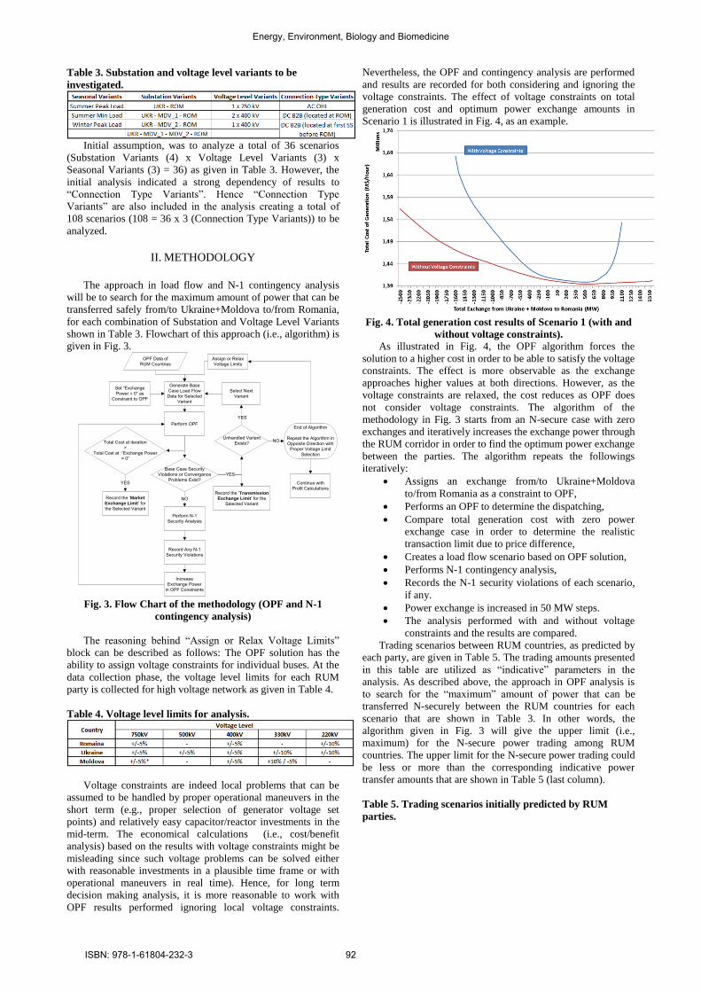
Table 3. Substation and voltage level variants to be

investigated.

Initial assumption, was to analyze a total of 36 scenarios

(Substation Variants (4) x Voltage Level Variants (3) x

Seasonal Variants (3) = 36) as given in Table 3. However, the

initial analysis indicated a strong dependency of results to

“Connection Type Variants”. Hence “Connection Type

Variants” are also included in the analysis creating a total of

108 scenarios (108 = 36 x 3 (Connection Type Variants)) to be

analyzed.

II. METHODOLOGY

The approach in load flow and N-1 contingency analysis

will be to search for the maximum amount of power that can be

transferred safely from/to Ukraine+Moldova to/from Romania,

for each combination of Substation and Voltage Level Variants

shown in Table 3. Flowchart of this approach (i.e., algorithm) is

given in Fig. 3. OPF Data of

RUM Countries

Generate Base Case Load Flow Data for Selected

Variant

Set “Exchange

Power = 0” as

Constraint to OPF

Perform OPF

Base Case Security Violations or Convergance

Problems Exist?

Select Next Variant

Perform N-1 Security Analysis

NO

Record Any N-1 Security Violations

Increase Exchange Power

in OPF Constraints

Record the ‘Transmission

Exchange Limit’ for the

Selected Variant

Unhandled Variant Exists?

YES

YES

End of Algorithm

Repeat the Algorithm in Opposite Direction with

Proper Voltage Limit Selection

NOTotal Cost at iteration >

Total Cost at “Exchange Power

= 0”

Record the ‘Market

Exchange Limit’ for

the Selected Variant

YES

Assign or Relax Voltage Limits

Continue with Profit Calculations

Fig. 3. Flow Chart of the methodology (OPF and N-1

contingency analysis)

The reasoning behind “Assign or Relax Voltage Limits”

block can be described as follows: The OPF solution has the

ability to assign voltage constraints for individual buses. At the

data collection phase, the voltage level limits for each RUM

party is collected for high voltage network as given in Table 4.

Table 4. Voltage level limits for analysis.

Voltage constraints are indeed local problems that can be

assumed to be handled by proper operational maneuvers in the

short term (e.g., proper selection of generator voltage set

points) and relatively easy capacitor/reactor investments in the

mid-term. The economical calculations (i.e., cost/benefit

analysis) based on the results with voltage constraints might be

misleading since such voltage problems can be solved either

with reasonable investments in a plausible time frame or with

operational maneuvers in real time). Hence, for long term

decision making analysis, it is more reasonable to work with

OPF results performed ignoring local voltage constraints.

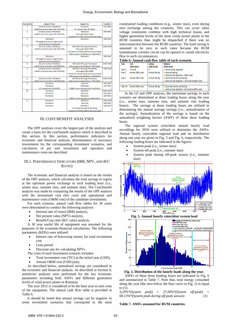
Nevertheless, the OPF and contingency analysis are performed

and results are recorded for both considering and ignoring the

voltage constraints. The effect of voltage constraints on total

generation cost and optimum power exchange amounts in

Scenario 1 is illustrated in Fig. 4, as an example.

Fig. 4. Total generation cost results of Scenario 1 (with and

without voltage constraints).

As illustrated in Fig. 4, the OPF algorithm forces the

solution to a higher cost in order to be able to satisfy the voltage

constraints. The effect is more observable as the exchange

approaches higher values at both directions. However, as the

voltage constraints are relaxed, the cost reduces as OPF does

not consider voltage constraints. The algorithm of the

methodology in Fig. 3 starts from an N-secure case with zero

exchanges and iteratively increases the exchange power through

the RUM corridor in order to find the optimum power exchange

between the parties. The algorithm repeats the followings

iteratively:

Assigns an exchange from/to Ukraine+Moldova

to/from Romania as a constraint to OPF,

Performs an OPF to determine the dispatching,

Compare total generation cost with zero power

exchange case in order to determine the realistic

transaction limit due to price difference,

Creates a load flow scenario based on OPF solution,

Performs N-1 contingency analysis,

Records the N-1 security violations of each scenario,

if any.

Power exchange is increased in 50 MW steps.

The analysis performed with and without voltage

constraints and the results are compared.

Trading scenarios between RUM countries, as predicted by

each party, are given in Table 5. The trading amounts presented

in this table are utilized as “indicative” parameters in the

analysis. As described above, the approach in OPF analysis is

to search for the “maximum” amount of power that can be

transferred N-securely between the RUM countries for each

scenario that are shown in Table 3. In other words, the

algorithm given in Fig. 3 will give the upper limit (i.e.,

maximum) for the N-secure power trading among RUM

countries. The upper limit for the N-secure power trading could

be less or more than the corresponding indicative power

transfer amounts that are shown in Table 5 (last column).

Table 5. Trading scenarios initially predicted by RUM

parties.

Energy, Environment, Biology and Biomedicine

ISBN: 978-1-61804-232-3 92

III. COST/BENEFIT ANALYSES

The OPF analyses cover the largest part of the analysis and

create a basis for the cost/benefit analysis which is described in

this section. In this section, performance indicators for

economic and financial analysis, determination of necessary

investments for the corresponding investment scenarios, and

calculation of per unit investment and operation and

maintenance costs are described.

III.1. PERFORMANCE INDICATORS (IRR, NPV, AND B/C

RATIO)

The economic and financial analysis is based on the results

of the OPF analysis, which calculates the total savings to region

at the optimum power exchange in each loading hour (i.e.,

winter max, summer max, and summer min). The Cost/benefit

analysis was made by comparing the results of the OPF analysis

with the investment cost (Inv cost) and operational and

maintenance costs (O&M cost) of the candidate investments.

For each scenario, annual cash flow tables for 30 years

were determined to conduct the following analyses:

Internal rate of return (IRR) analysis,

Net present value (NPV) analysis,

Benefit/Cost ratio (B/C ratio) analysis.

A 30 year useful life of equipment was assumed for the

purposes of the economic/financial calculations. The following

parameters (KEPs) were utilized:

Interest rate of borrowing money for total investment

cost

Loan period

Discount rate for calculating NPVs

The costs of each investment scenario includes:

Total investment cost (TIC) at the initial year (USD),

Annual O&M cost (USD/year).

As described below, annualized savings are considered in

the economic and financial analysis. As described in Section 9,

sensitivity analyses were performed for the key economic

parameters including both AWFs and different generation

levels of wind power plants in Romania.

The year 2012 is considered to be the base year in unit costs

of the equipment. The annual cash flow table is provided in

Table 6.

It should be noted that annual savings can be negative in

some investment scenarios that correspond to the most

constrained loading conditions (e.g., winter max), even during

zero exchange among the countries. This can occur when

voltage constraints combine with high technical losses, and

higher generation levels of the most costly power plants in the

RUM countries than might be dispatched if there was no

interconnection between the RUM countries. The total saving is

assumed to be zero in such cases because the RUM

transmission corridor circuit can be opened to curtail electricity

flow in such circumstances.

Table 6. Annual cash flow table of each scenario.

In the LF and OPF analysis, the maximum savings in each

scenario are determined at three loading hours along the year

(i.e., winter max, summer max, and summer min loading

hours). The savings at these loading hours are utilized in

determining the annual average savings (i.e., annualization of

the savings). Annualization of the savings is based on the

annualized weighting factors (AWF) of these three loading

hours.

The regional system coincident annual hourly load

recordings for 2010 were utilized to determine the AWFs.

Annual hourly coincident regional load and its distribution

along one year are given in Fig. 5 and Fig. 6, respectively. The

following loading hours are indicated in the figures:

System peak (i.e., winter max)

System off-peak (i.e., summer min)

System peak during off-peak season (i.e., summer

max)

Fig. 5. Annual hourly coincident system load

Fig. 5. Distribution of the hourly loads along the year.

AWFs of these three loading hours are indicated in Fig. 6

and summarized in Table 7. Note that, total energy consumed

along the year (the area below the blue curve in Fig. 5) is equal

to (1):

4,29%*(System peak) + 27,58%*(System off-peak) +

68,13%*(System peak during off-peak season) (1)

Table 7. AWFs assumed for RUM countries.

Energy, Environment, Biology and Biomedicine

ISBN: 978-1-61804-232-3 93

Loading condition Loading hour AWFs

System peak Winter max 4,29%

System off-peak Summer min 27,58%

System peak during off-peak season

Summer max 68,13%

This approach is analyzed below for the following

parameter and investment scenario (Case_VC-I_W30%):

Investment Scenario No: 1

o 1x400kV Ukraine-MDV_2-ROM

(connection through HVDC B2B substation

at Romania)

Wind generation level at Romania: 30%

Voltage constraints: Ignored

Loading Scenarios:

o Scenario 4: System peak (Winter max)

o Scenario 3: System off-peak (Summer min)

o Scenario 2: System peak during off-peak

season (Summer max)

The savings which are determined by OPF analyses for the

three loading scenarios are given in Table 8.

Table 8. Annualization of savings for the Scenarios 2,3 and

4

As illustrated in the table:

The maximum saving occurs at “system peak” (i.e.,

winter max).

o The room for OPF is maximum given high

generation levels of cost-ineffective power

plants in the region.

The minimum saving occurs at “system off-peak”

(i.e., summer min).

o The potential for optimization is minimal

due to system constraints at minimum

loading conditions

o The availability of cost effective generator

capacity in the system is minimum.

In order to determine the annualized total saving,

availability of the line should be estimated (downtime

for maintenance and unavailability of the line due to

faults must be estimated). An availability of 8322

hours, which corresponds to 95% of the hours in a

year, is assumed for the economic/financial analysis.

Annual saving for this investment scenario is

calculated as 43.596.276,03 USD/year, as illustrated

in Table 8.

This approach was employed in for investment scenarios to

in determine the annualized savings for cost/benefit analysis.

III.2. NECESSARY INVESTMENTS AND CORRESPONDING COSTS

This section reviews the approach to determining the total

amount of equipment that should be installed to support each

investment scenario. The following assumptions are made:

Each substation was equipped with a spare bay at the

corresponding voltage level, in case of

emergency/maintenance/etc.;

750/400 kV or 750/330 kV transformers at the

corresponding substations to satisfy n-1 reliability

criteria;

In the scenarios in which there are two substations in

Moldova, there will be only one transformer in each

substation. This meant that n-1 contingency was

satisfied by the transformer in the other substation;

and

As the intermediary substations in the corridor, the

new substations in Moldova were assumed to have

additional bays- the total number of which depends

on the connection type.

The determination of the necessary equipment for different

investment scenarios is described in the following subsections.

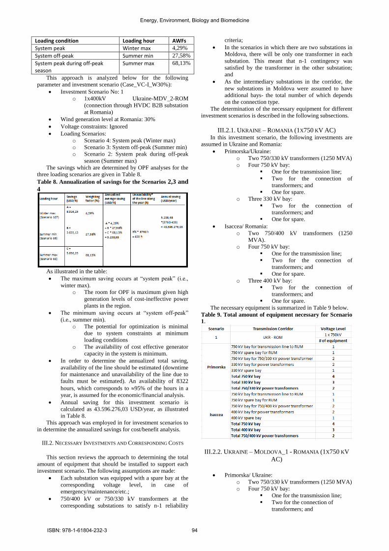
III.2.1. UKRAINE – ROMANIA (1X750 KV AC) In this investment scenario, the following investments are

assumed in Ukraine and Romania:

Primorska/Ukraine:

o Two 750/330 kV transformers (1250 MVA)

o Four 750 kV bay:

One for the transmission line;

Two for the connection of

transformers; and

One for spare.

o Three 330 kV bay:

Two for the connection of

transformers; and

One for spare.

Isaccea/ Romania:

o Two 750/400 kV transformers (1250

MVA).

o Four 750 kV bay:

One for the transmission line;

Two for the connection of

transformers; and

One for spare.

o Three 400 kV bay:

Two for the connection of

transformers; and

One for spare.

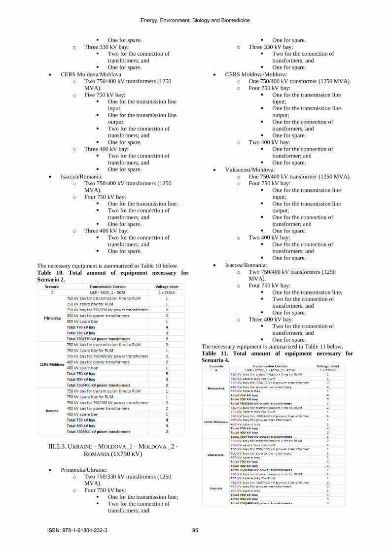
The necessary equipment is summarized in Table 9 below.

Table 9. Total amount of equipment necessary for Scenario

1.

III.2.2. UKRAINE – MOLDOVA_1 - ROMANIA (1X750 KV

AC)

Primorska/ Ukraine:

o Two 750/330 kV transformers (1250 MVA)

o Four 750 kV bay:

One for the transmission line;

Two for the connection of

transformers; and

Energy, Environment, Biology and Biomedicine

ISBN: 978-1-61804-232-3 94

One for spare.

o Three 330 kV bay:

Two for the connection of

transformers; and

One for spare.

CERS Moldova/Moldova:

o Two 750/400 kV transformers (1250

MVA).

o Five 750 kV bay:

One for the transmission line

input;

One for the transmission line

output;

Two for the connection of

transformers; and

One for spare.

o Three 400 kV bay:

Two for the connection of

transformers; and

One for spare.

Isaccea/Romania:

o Two 750/400 kV transformers (1250

MVA).

o Four 750 kV bay:

One for the transmission line;

Two for the connection of

transformers; and

One for spare.

o Three 400 kV bay:

Two for the connection of

transformers; and

One for spare.

The necessary equipment is summarized in Table 10 below.

Table 10. Total amount of equipment necessary for

Scenario 2.

III.2.3. UKRAINE – MOLDOVA_1 – MOLDOVA _2 -

ROMANIA (1X750 KV)

Primorska/Ukraine:

o Two 750/330 kV transformers (1250

MVA).

o Four 750 kV bay:

One for the transmission line;

Two for the connection of

transformers; and

One for spare.

o Three 330 kV bay:

Two for the connection of

transformers; and

One for spare.

CERS Moldova/Moldova:

o One 750/400 kV transformer (1250 MVA).

o Four 750 kV bay:

One for the transmission line

input;

One for the transmission line

output;

One for the connection of

transformers; and

One for spare.

o Two 400 kV bay:

One for the connection of

transformer; and

One for spare.

Vulcanesti/Moldova:

o One 750/400 kV transformer (1250 MVA).

o Four 750 kV bay:

One for the transmission line

input;

One for the transmission line

output;

One for the connection of

transformer; and

One for spare.

o Two 400 kV bay:

One for the connection of

transformers; and

One for spare.

Isaccea/Romania:

o Two 750/400 kV transformers (1250

MVA).

o Four 750 kV bay:

One for the transmission line;

Two for the connection of

transformers; and

One for spare.

o Three 400 kV bay:

Two for the connection of

transformers; and

One for spare.

The necessary equipment is summarized in Table 11 below.

Table 11. Total amount of equipment necessary for

Scenario 4.

Energy, Environment, Biology and Biomedicine

ISBN: 978-1-61804-232-3 95

IV. HVDC BACK TO BACK CONNECTION

ANALYSES

In this section, first the challenges with the HVAC

interconnection of ENTSO-E and IPS/UPS systems are

discussed. Then, the analysis for the HVDC interconnections of

RUM Countries is presented. Romania is connected to the

ENTSO-E system, whereas Ukraine and Moldova are

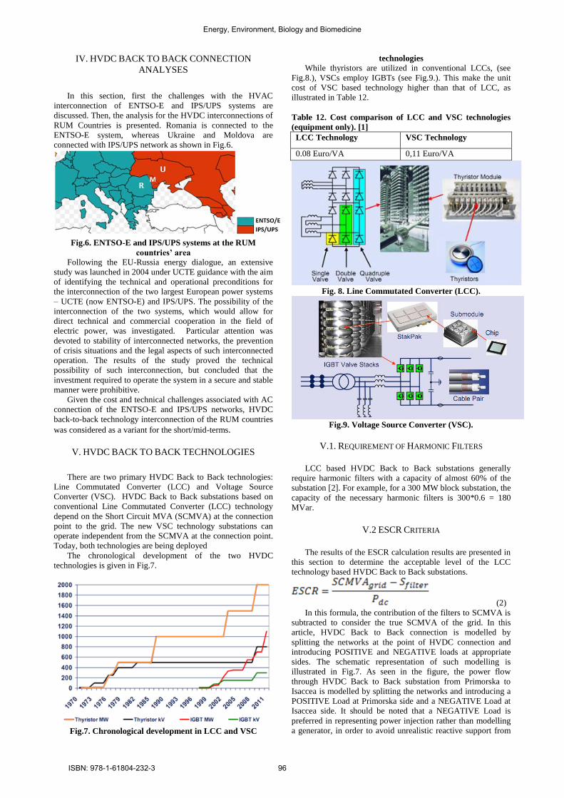
connected with IPS/UPS network as shown in Fig.6.

Fig.6. ENTSO-E and IPS/UPS systems at the RUM

countries’ area

Following the EU-Russia energy dialogue, an extensive

study was launched in 2004 under UCTE guidance with the aim

of identifying the technical and operational preconditions for

the interconnection of the two largest European power systems

– UCTE (now ENTSO-E) and IPS/UPS. The possibility of the

interconnection of the two systems, which would allow for

direct technical and commercial cooperation in the field of

electric power, was investigated. Particular attention was

devoted to stability of interconnected networks, the prevention

of crisis situations and the legal aspects of such interconnected

operation. The results of the study proved the technical

possibility of such interconnection, but concluded that the

investment required to operate the system in a secure and stable

manner were prohibitive.

Given the cost and technical challenges associated with AC

connection of the ENTSO-E and IPS/UPS networks, HVDC

back-to-back technology interconnection of the RUM countries

was considered as a variant for the short/mid-terms.

V. HVDC BACK TO BACK TECHNOLOGIES

There are two primary HVDC Back to Back technologies:

Line Commutated Converter (LCC) and Voltage Source

Converter (VSC). HVDC Back to Back substations based on

conventional Line Commutated Converter (LCC) technology

depend on the Short Circuit MVA (SCMVA) at the connection

point to the grid. The new VSC technology substations can

operate independent from the SCMVA at the connection point.

Today, both technologies are being deployed

The chronological development of the two HVDC

technologies is given in Fig.7.

Fig.7. Chronological development in LCC and VSC

technologies

While thyristors are utilized in conventional LCCs, (see

Fig.8.), VSCs employ IGBTs (see Fig.9.). This make the unit

cost of VSC based technology higher than that of LCC, as

illustrated in Table 12.

Table 12. Cost comparison of LCC and VSC technologies

(equipment only). [1]

LCC Technology VSC Technology

0.08 Euro/VA 0,11 Euro/VA

Fig. 8. Line Commutated Converter (LCC).

Fig.9. Voltage Source Converter (VSC).

V.1. REQUIREMENT OF HARMONIC FILTERS

LCC based HVDC Back to Back substations generally

require harmonic filters with a capacity of almost 60% of the

substation [2]. For example, for a 300 MW block substation, the

capacity of the necessary harmonic filters is 300*0.6 = 180

MVar.

V.2 ESCR CRITERIA

The results of the ESCR calculation results are presented in

this section to determine the acceptable level of the LCC

technology based HVDC Back to Back substations.

(2)

In this formula, the contribution of the filters to SCMVA is

subtracted to consider the true SCMVA of the grid. In this

article, HVDC Back to Back connection is modelled by

splitting the networks at the point of HVDC connection and

introducing POSITIVE and NEGATIVE loads at appropriate

sides. The schematic representation of such modelling is

illustrated in Fig.7. As seen in the figure, the power flow

through HVDC Back to Back substation from Primorska to

Isaccea is modelled by splitting the networks and introducing a

POSITIVE Load at Primorska side and a NEGATIVE Load at

Isaccea side. It should be noted that a NEGATIVE Load is

preferred in representing power injection rather than modelling

a generator, in order to avoid unrealistic reactive support from

Energy, Environment, Biology and Biomedicine

ISBN: 978-1-61804-232-3 96

the HVDC Back to Back via the generator. Given this

representation, the SCMVA contribution of the HVDC Back to

Back filters is not considered in the load flow and short circuit

analysis. Therefore, the ESCR should be calculated as in (3).

(3)

For the secure operation of HVDC Back to Back substation

that is based on LCC the

ESCR 3 (base case) [3] (4)

Essentially, the ESCR is different at each connection point

of the HVDC Back to Back substations given different

topologies. For the sake of security, the minimum value among

the SCMVA at each connection point is considered in

calculating of the ESCRs. The available HVDC Back to Back

substation capacity is calculated assuming that total capacity of

the substation is formed by 300 MW blocks, while taking into

account the ESCR criteria (4).

V.3 DETERMINATION OF TOTAL CAPACITY OF HVDC

BACK TO BACK SUBSTATION

It is assumed that the HVDC Back to Back substation

blocks will be in the order of 300 MW capacities. The

following arguments support this approach:

300 MW capacity HVDC Back to Back substations

are available in the market.

The order of 300 MW is plausible to match the

optimum substation capacity with the optimum power

exchange amounts that are determined in LF (Load

Flow) and OPF (Optimal Power Flow) analysis.

For example, the approach in determining the total capacity

of the HVDC Back to Back substation is presented below

(1x400 kV transmission line between Ukraine - Romania

through HVDC Back to Back substation in Ukraine):

Loading condition of the scenario: Summer

maximum.

Wind generation level in Romania: Normal (i.e.,

generation level of the wind power plants in

Dubrudja/ROM region is 30% of the capacity).

OPF results at base case (i.e., ignoring N-1

contingency):

o 700 MW ( Ukraine => Romania)

N-1 security exchange technical limit:

o 1.300 MW ( Ukraine => Romania)

o Since 700 < 1300, 700 MW power

exchange is feasible in the sense of N-1

security concern.

Voltage collapse power exchange limit:

o 1.500 MW ( Ukraine => Romania)

o Since 700 < 1.500, 700 MW power

exchange is feasible in the sense of voltage

collapse concern.

Assuming that HVDC Back to Back substation is

composed of 300 MW blocks, total number of block

to realize 700 MW power exchange is three (3*300 =

900 > 700)

o Total capacity of the HVDC BACK TO

BACK substation is 900 MW.

ESCR criteria:

o Maximum SCMVA of the grid at the

HVDC Back to Back substation is

calculated as 2.063 MVA

o ESCR = 2.063/900 = 2,29

o Since 2,29 < 3, total capacity of 900 MW is

NOT acceptable in the sense of ESCR

criteria.

o If one block among the three blocks is

removed, then the total capacity of the

substation is 2x300 = 600 MW

ESCR = 2.063/600 = 3,43 > 3 =>

acceptable

An HVDC Back to Back capacity of 600 MW is proven in

the summer maximum loading conditions. Similar analyses

were performed for winter maximum and summer minimum

loading conditions, as well. The total capacity of the HVDC

Back to Back substation is considered to be the maximum

capacity determined among three loading scenarios. This

approach is considered in all scenarios that include HVDC

Back to Back substation.

VI. CONCLUSIONS

Voltage constraints were local problems that could be

resolved through network operations in the short term (e.g.,

proper selection of generator voltage set points) and relatively

inexpensive capacitor/reactor investments in the mid-term.

Hence, voltage constraints are ignored in certain cases to

determine the maximum volume of power exchange among the

countries. The maximum voltage deviation at the key nodes

was observed to be +/-20%, which could be resolved by proper

compensation through the provision of additional reactors.

The increase in wind generation in Romania dramatically

limited the ability of the RUM countries to optimize the

regional generation fleet based on the cost of production. In

some investment scenarios, the flow of power changed

direction from north south to south north when the wind

power plant generation in Romania increased from 30% to 70%

and it is designated as must run. This occurs when the OPF

algorithm forced inefficient high cost generators, first in

Romania and then in Moldova and Ukraine, to reduce their

generation in favor of must run wind. This process continued

until the reduction of generation in Ukraine and Moldova

became so much more cost effective than the reduction of

generation in Romania that the power flow changed direction.

From this point onward, Romania began exporting power in a

northward direction to Moldova and Ukraine.

It is important to note that for the investment scenario of a

400 kV connection passing through a HVDC B2B substation,

the benefit/cost ratio was > 1, when Romanian must run wind

generation was modeled with a 30% capacity factor.

Connection through the HVDC Back to Back was superior

to connection through AC options in almost every investment

scenario considered. This was because the HVDC connection

reduced technical network constraints to increase power

exchange, enlarging the scope for power flows in the sub-

region.

In fact, HVDC B2B was the only investment solution which

resulted in benefit/cost > 1 when considering the scenario of

Romanian must run operating with a 30% capacity factor. And,

the technical challenges to synchronizing the current IPS/UPS

and ENTSO-E members of the RUM working group would

inhibit interconnection via high voltage AC interconnections for

the foreseeable future. Therefore, HVDC technology based

interconnection of the RUM countries seemed the most rational

solution in the short/mid-term.

There was no significant difference revealed in the

cost/benefit analyses for the different investment scenarios

related to the configuration of the corridor, i.e., either directly

from Ukraine to Romania or through Moldova. If the

interconnection between RUM countries were realized in

intermediate steps, (for example, if the connection between

Romania and Moldova were realized before all three countries

are interconnected), energy trade between Romania and

Moldova could begin before the trading among all three

countries by directing a generator in Moldova to operate

synchronously with Romania in island mode.

Energy, Environment, Biology and Biomedicine

ISBN: 978-1-61804-232-3 97

REFERENCES

[1]. Lazaros P. Lazaridis, “Economic Comparison of HVAC and

HVDC Solutions for Large Offshore Wind Farms under Special

Consideration of Reliability”, Master’s Thesis, Royal Institute

of Technology Department of Electrical Engineering,

Stockholm 2005.

[2]. Dodds, B. Railing, K. Akman, B. Jacobson, T. Worzyk,

“HVDC VSC (HVDC light) transmission – operating

experiences,” CIGRE 2010.

[3]. “Feasibility study of the asynchronous interconnection

between the power systems of Iran and Turkey”, Interim

Report, Professor Francesco Iliceto, Consultant to TEIAS,

Rome (Italy), November 2009.

* Siemens PTI Documentation

Energy, Environment, Biology and Biomedicine

ISBN: 978-1-61804-232-3 98