TRANSMISSION COMPUTATIONAL MODEL IN SIMULINKpernerscontacts.upce.cz/33_2013/Kucera.pdf · Number 4, Volume VIII, December 2013 Kučera, Píštěk: Transmission Computational model

Number 4, Volume VIII, December 2013

Kučera, Píštěk: Transmission Computational model in Simulink 37

TRANSMISSION COMPUTATIONAL MODEL IN SIMULINK

Pavel Kučera1, Václav Píštěk2

Summary: The article describes the creation of a transmission and a clutch computational model. These parts of the powertrain are created using basic blocks from the Simulink library, with the input values obtained from the manufacturer. The description of a computational model and its setup in Simulink software is presented in this article. In the end, the evaluation of two simulations of gear shifting and running the transmission on the dynamometer is discussed.

Key words: Transmission, Clutch, Synchronizers, Gear Shift, Computational Model

INTRODUCTION

Recent development of mechanical and mechatronic systems was considerably accelerated by the introduction of virtual applications which prevent many possible complications during the process of translating the designed mechanism or construction element into production. The support from software developers in the form of various computer programmes and pre-prepared codes for development and testing of the design is immense. Such software allows the assembly of dynamic systems from blocks and elements included in the libraries, substituting various parts of computational models, or the creation of the computational model from basic elements which then form various subsystems akin to blocks included in the special libraries of the development applications.

This article deals with the development of a transmission and clutch computational model of a commercial vehicle. The model is assembled from the blocks included in the libraries of Simulink software and follows the computational model of an engine described in the previous article (3). When connected, these models provide the capability of simulating a large part of the vehicle’s powertrain. This powertrain model will then be developed even further.

The model was created in Simulink software which offers a vast support for simulating parts of a powertrain. The application environment is able of both running the simulations and subsequent post-processing of the results in Matlab. The computational model could also be run at real-time testing hardware.

1 Ing. Pavel Kučera, Brno University of Technology, Faculty of Mechanical Engineering, Institute of Automotive Engineering, Technická 2896/2 , 616 69 Brno, Tel.: +420 541 142 252, Fax: +420 541 143 354, E-mail: [email protected] 2 prof. Ing. Václav Píštěk, DrSc., Brno University of Technology, Faculty of Mechanical Engineering, Institute

of Automotive Engineering, Technická 2896/2 , 616 69 Brno, Tel.: +420 541 142 271, Fax: +420 541 143 354, E-mail: [email protected]



1. BASIC EQUATIONS OF THE COMPUTATIONAL MODEL

1.1 Clutch The computational model simulates the clutch of a commercial vehicle (see Fig. 1)

which comprises a friction plate, a pressure plate and a diaphragm spring. Its actuation is mechanical, with pneumatic power. The clutch model structure is simplified to describe the transfer of the torque originating from the preload of the spring and controlled by the input force.

Source: (5)

Fig. 1 – The clutch of a commercial vehicle

There are two possible approaches to clutch calculations. The first utilizes the premise of even clutch wear while the second assumes an even pressure distribution on the clutch friction lining. The equations taken from the literature (4) are presented below. For the even clutch wear the equation can be written as

(1)

where p is the pressure acting on the lining of radius r, pa is the maximum pressure on the lining and d is the diameter on which the maximum pressure acts. The relationship between pressure and radius is hyperbolic. The force on the friction lining is

(2)

where Dc is the lining’s outer diameter, dc is the lining’s inner diameter and rc is the clutch radius. In that case, the torque transferred by the clutch is

(3)

where fc is the friction coefficient of the lining, ranging from 0.3 to 0.4. Incorporating Eq. (2), Eq. (3) can be modified as

(4)

The assumption of even pressure distribution on the clutch friction lining can be written as:

(5)

Therefore, the force on the friction lining is:



2 (6)

While the torque transferred by the clutch is:

2 (7)

with the individual symbols described above. Incorporating Eq. (6), Eq. (7) can be modified as:

(8)

1.2 Transmission The transmission of commercial vehicles is usually composed of several gearboxes. The

computational model describes transmission made up of components where normal and reduction gears are selected and also the main gearbox (see Fig. 2) with five forward gear ratios and one reverse gear ratio. The main gearbox is connected to an auxiliary gearbox comprising two gear ratios used to broaden the range of main gear ratios. The driver can therefore choose from seven forward gear ratios, where the first five are selected in the main gearbox and the additional 6th and 7th can be selected as follows: when the driver pushes the gear lever to the right, the sensor sends a signal to pneumatic actuator, which selects the second gear in the auxiliary gearbox and the driver proceeds to select 4th gear in the main gearbox. The same applies for selecting 7th gear, where 5th gear is selected in the main gearbox and 2nd in the auxiliary gearbox. The driver has a further option in selecting a reduction gear, which makes it a total of fourteen forward gear ratios and two reverse gear ratios.

Source: (5)

Fig. 2 – Main gearbox of a commercial vehicle

Transmission parts contain gear wheels. Their gear ratios are calculated according to the following equation

1, 2, 3, … (9)

where zn is the number of teeth of the gear wheel. As the gearboxes accommodate synchronizers, their function will be included in the computational model. The description of their working principle follows the same path as



with the clutch but takes into account the difference caused by the fact that the surfaces are chamfered, typically at an angle of 7°. The synchronizer ring calculation is depicted in Fig. 3.

Source (4)

Fig. 3 – Forces acting on a synchronizer ring

Again, there are two possible approaches to the calculations: one with the even wear assumption and the other with the even pressure distribution assumption. The first possibility with even wear is described using equations from the literature (4) as written below. The assumption is the same as in Eq. (1) for the clutch.

Therefore, the force acting on the synchronizer ring is

sin (10)

where α is the chamfer angle of the synchronizer ring, Ds is the ring’s outer diameter, dc is the ring’s inner diameter, pa is the maximum pressure on the ring and rs is the ring’s radius. The torque transferred by the synchronizer ring is

(11)

where fs is the friction coefficient of the surface of the ring, ranging from 0.08 to 0.1 according to the used oil. Incorporating Eq. (10), Eq. (11) can be modified as

(12)

In the case of the even pressure distribution assumption, the force on the synchronizer ring is

sin 2 (13)

similar to Eq. (5) regarding the clutch. The torque transferred by the synchronizer ring according to the even pressure distribution assumption is

(14)

with the individual symbols described above. Incorporating Eq. (13), Eq. (14) can be modified as

(15)



A rigid connection of the desired gear and the shaft is ensured by dog clutches. Their inclusion in the computational model offers the settings of engaged or disengaged state and their stiffness and damping properties. The synchronizing begins when the driver operates the gear lever, which is translated by a mechanical gear with pneumatic servomotor into force acting on the outer body of the synchronizer’s dog clutch. Between the dog clutch body and synchronizer rings, there is a ball with a spring (detent) which transfers the force on the ring itself. That results in the interaction between the synchronizer rings, adjusting the speeds of the shafts. By pushing the ball even further, the force on the rings grows due to the presence of the spring. After the ball travels all of its available distance, there is no further synchronization going on, but the dog clutch is now free to move so that it connects with the gear wheel on the opposite side of the dog clutch. This ends the whole process and the gear wheel which previously rotated freely is now rigidly connected with the shaft.

The force transferred by the detent can be calculated according to the following equation

∝ ∝

∝ ∝

(16)

where Fy is the force from the spring, αb is the tilt angle of the face which is in contact with the ball, µb is the friction coefficient between the ball and adjacent surfaces and ns is the number of detent within the synchronizer. The calculated force Fx is then equal to the force acting on the synchronizer rings. The synchronizing time is described by equation

(17)

where ts is the synchronizing time, J1 is the moment of inertia of the drive shaft, 2 is the

angular velocity of the drive shaft, J2 is the moment of inertia of the driven shaft, 2 is the

angular velocity of the driven shaft and Ms is the synchronizing moment. The angular velocity of the drive shaft after synchronization is

(18)

2. COMPUTATIONAL MODEL

2.1 Subsystems The computational model was created using the blocks included in the Simulink

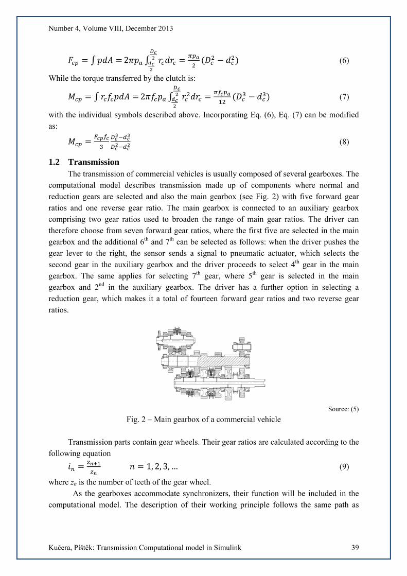
libraries with the help of literature (1), (2), (3). Selected predefined blocks which represent parts of the powertrain are shown in Fig. 4.



Source: Author

Fig. 4 – Selected blocks from Simulink libraries One of the main blocks is the double-sided synchronizer. It is made up of several other

blocks representing construction elements for revolution synchronization, specifically the dog clutch, synchronizer rings and a ball-spring coupling so-called detent. The blocks allow the user to set required input data for the synchronizer’s construction elements. Furthermore, these blocks can be connected with other blocks representing the gear and the user is able to assemble the desired gearbox configuration.

Source: Author

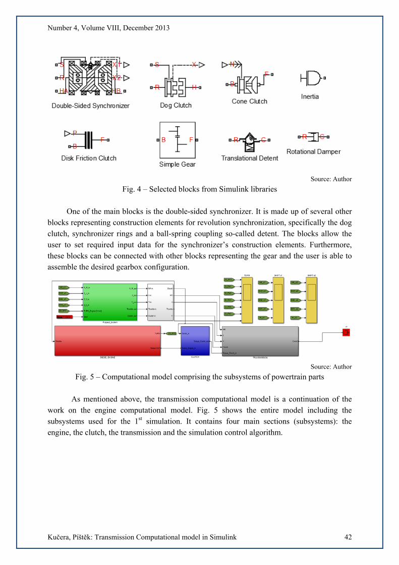
Fig. 5 – Computational model comprising the subsystems of powertrain parts

As mentioned above, the transmission computational model is a continuation of the work on the engine computational model. Fig. 5 shows the entire model including the subsystems used for the 1st simulation. It contains four main sections (subsystems): the engine, the clutch, the transmission and the simulation control algorithm.



Source: Author

Fig. 6 – Computational model of the clutch

The clutch model is presented in Fig. 6. It was created using a Simulink library block which works according to the even pressure distribution assumption from equations in Chapter 1. Elements representing the spring preload and an input for the regulating force were added to the block.

Source: Author

Fig. 7 – Computational model of the transmission The transmission computational model is depicted in Fig. 7 and contains the main

gearbox, where main gears and normal or reduction gear can be selected, and the auxiliary gearbox, which adds next two gear ratios to the main five. The green blocks represent individual gear ratios in the transmission while the blue blocks stand for the synchronizers between individual gear wheels. Synchronization calculation follows the equations in Chapter 1 for even pressure distribution assumption and the equations for forces transferred by detent. In this block, only the maximum force transferrable by this detent can be set. The gear change can be controlled by the regulating force input in the synchronizer block, or by the speed



input, which is then integrated and the dog clutch housing position within the synchronizer is determined. This approach was used in the red block in Fig.7 which controls the selection of all gear ratios. Its inner structure is shown in Fig. 8. The X and Y coordinates determining the gear selector fork position enter the block. The X coordinate determines the synchronizer movement while the Y coordinate determines which synchronizer will be operated. Reduction gear is preselected by sending a logical 1 or 0 into the block. The chosen number gives a signal to change gear, but the process starts only after the clutch is depressed. The algorithm and set gear change time then control the synchronizer´s movement and therefore the change of gear ratio. The last part of the algorithm describes the selection of 6th and 7th gear, which starts after pushing the gear lever to the right. That means the Y input reaches its maximum value in the computational model. This is followed by a gear change in the auxiliary gearbox and the selection of 4th or 5th gear in the main gearbox. A synchronizer movement time is also set for this case. The overall gear change time from the moment of clutch pedal depression to its release is set to 1.1 s. The gear change algorithm is assembled from the basic Simulink elements and does not use pre-prepared blocks.

Source: Author

Fig. 8 – The synchronizer control algorithm in the transmission computational model

3. SIMULATION BY COMPUTATIONAL MODEL

The simulations were set up with a fixed step while the ode14x solver, which combines Newton and extrapolation methods, was used for the computation. This solver is recommended for the elements included in the computational model.

3.1 Control algorithm and gear change simulation The control algorithm is shown in Fig. 9. This subsystem is tasked with the control of

the clutch, engine and transmission computational model. The simulation starts with the



engine idling at 800 rpm, 1st reduction gear selected and clutch pedal depressed. After 1 s of simulation time, the clutch begins to engage and the throttle builds up, causing the rotation of individual transmission shafts. The algorithm continues to control the simulation so that when the engine reaches its maximum speed, the throttle value falls to zero, the clutch disengages and the selection of a higher gear ratio starts. At the moment the dog clutch of a synchronizer reaches the position of a selected gear, a signal to open the throttle and engage the clutch is sent. This procedure is repeated until the selection of the highest gear ratio. The results of this simulation are presented in Fig. 10 and Fig. 11, showing the speed curve and the position of individual synchronizers in time for duration of 30 s respectively.

Source: Author

Fig. 9 – 1st simulation algorithm

The results show the speeds of the engine and individual transmission shafts. The drops in speed are caused by the process of synchronizing of the shafts. The output speed curve would be smoother if further powertrain parts such as axles or a tire model were incorporated in the computational model, as they would cause both the output speed of the entire powertrain and the shaft speed curves to be flattened due to the inertia of the vehicle.

Source: Author

Fig. 10 – Speed curves of individual transmission parts (1st simulation)



The maximum output speed for an engine speed of 1950 rpm in the computational

model is 3189 rpm, which agrees with an analytical calculation. The results also prove that the gear change time set in the simulation is sufficient from the speed drop point of view, so that the engine speed after the gear change does not fall below the value where maximum engine torque occurs.

Source: Author

Fig. 11 – The dog clutch position within the synchronizer (1st simulation)

3.2 Simulation including a dynamometer The simulation with a dynamometer (Fig. 12) is executed with the 3rd reduction gear

selected and with the engine throttle fully opened.

Source: Author

Fig. 12 – The computational model comprising the subsystems and a dynamometer (2nd simulation)

The entire computational model is connected to a dynamometer model which is

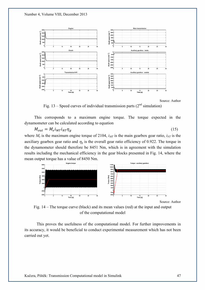
adjusted to brake the powertrain to achieve 1100 rpm engine speed. Fig. 13 shows the speed curves for individual parts of the powertrain gathered from simulation with dynamometer.



Source: Author

Fig. 13 – Speed curves of individual transmission parts (2nd simulation)

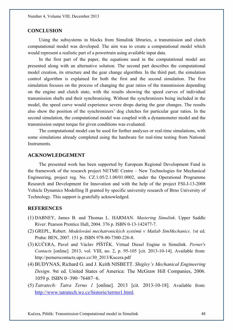
This corresponds to a maximum engine torque. The torque expected in the dynamometer can be calculated according to equation

(15)

where Me is the maximum engine torque of 2104, iMT is the main gearbox gear ratio, iNT is the

auxiliary gearbox gear ratio and g is the overall gear ratio efficiency of 0.922. The torque in

the dynamometer should therefore be 8451 Nm, which is in agreement with the simulation results including the mechanical efficiency in the gear blocks presented in Fig. 14, where the mean output torque has a value of 8450 Nm.

Source: Author

Fig. 14 – The torque curve (black) and its mean values (red) at the input and output of the computational model

This proves the usefulness of the computational model. For further improvements in its accuracy, it would be beneficial to conduct experimental measurement which has not been carried out yet.



CONCLUSION

Using the subsystems in blocks from Simulink libraries, a transmission and clutch computational model was developed. The aim was to create a computational model which would represent a realistic part of a powertrain using available input data.

In the first part of the paper, the equations used in the computational model are presented along with an alternative solution. The second part describes the computational model creation, its structure and the gear change algorithm. In the third part, the simulation control algorithm is explained for both the first and the second simulation. The first simulation focuses on the process of changing the gear ratios of the transmission depending on the engine and clutch state, with the results showing the speed curves of individual transmission shafts and their synchronizing. Without the synchronizers being included in the model, the speed curve would experience severe drops during the gear changes. The results also show the position of the synchronizers’ dog clutches for particular gear ratios. In the second simulation, the computational model was coupled with a dynamometer model and the transmission output torque for given conditions was evaluated.

The computational model can be used for further analyses or real-time simulations, with some simulations already completed using the hardware for real-time testing from National Instruments.

ACKNOWLEDGEMENT

The presented work has been supported by European Regional Development Fund in the framework of the research project NETME Centre – New Technologies for Mechanical Engineering, project reg. No. CZ.1.05/2.1.00/01.0002, under the Operational Programme Research and Development for Innovation and with the help of the project FSI-J-13-2008 Vehicle Dynamics Modelling II granted by specific university research of Brno University of Technology. This support is gratefully acknowledged.

REFERENCES

(1) DABNEY, James B. and Thomas L. HARMAN. Mastering Simulink. Upper Saddle River: Pearson Prentice Hall, 2004. 376 p. ISBN 0-13-142477-7.

(2) GREPL, Robert. Modelování mechatronických systémů v Matlab SimMechanics. 1st ed. Praha: BEN, 2007. 151 p. ISBN 978-80-7300-226-8.

(3) KUČERA, Pavel and Václav PÍŠTĚK. Virtual Diesel Engine in Simulink. Perner's Contacts [online]. 2013, vol. VIII, no. 2, p. 95-105 [cit. 2013-10-14]. Available from: http://pernerscontacts.upce.cz/30_2013/Kucera.pdf

(4) BUDYNAS, Richard G. and J. Keith NISBETT. Shigley’s Mechanical Engineering Design. 9st ed. United States of America: The McGraw Hill Companies, 2006. 1059 p. ISBN 0−390−76487−6.

(5) Tatratech: Tatra Terno 1 [online]. 2013 [cit. 2013-10-18]. Available from: http://www.tatratech.wz.cz/historie/terrno1.html.

Documents

TRANSMISSION COMPUTATIONAL MODEL IN SIMULINKpernerscontacts.upce.cz/33_2013/Kucera.pdf · Number 4, Volume VIII, December 2013 Kučera, Píštěk: Transmission Computational model