Transition waves in bistable structures. II. Analytical

1

3

5

7

9

11

13

15

17

19

21

23

25

27

29

31

33

35

37

39

41

43

45

ARTICLE IN PRESS

3B2v8:06a=w ðDec 5 2003Þ:51cXML:ver:5:0:1 MPS : 1178 Prod:Type:FTP

pp:1230ðcol:fig::NILÞED:VinuthaM:B:

PAGN:Ashok SCAN:Raj

Journal of Mechanics and Physics of solids

] (]]]]) ]]]–]]]

U0022-5096/$ -

doi:10.1016/j

�CorrespoE-mail ad

1Also for c

www.elsevier.com/locate/jmps

ROOF

Transition waves in bistable structures. II.Analytical solution: wave speed and energy

dissipation

Leonid Slepyana, Andrej Cherkaevb,1, Elena Cherkaevb,�

aDepartment of Solid Mechanics, Materials and Systems, Tel Aviv University, Ramat Aviv 69978, IsraelbDepartment of Mathematics, The University of Utah, 155 South 1400 East, JWB233, Salt Lake City, UT

84112, USA

Received 30 January 2004; received in revised form 2 August 2004; accepted 7 August 2004

CORRECTED PAbstract

We consider dynamics of chains of rigid masses connected by links described by irreversible,

piecewise linear constitutive relation: the force–elongation diagram consists of two stable

branches with a jump discontinuity at the transition point. The transition from one stable state

to the other propagates along the chain and excites a complex system of waves. In the first part

of the paper (Cherkaev et al., Transition waves in bistable structures. I. Delocalization of

damage), the branches could be separated by a gap where the tensile force is zero, the

transition wave was treated as a wave of partial damage. Here we assume that there is no zero-

force gap between the branches. This allows us to obtain steady-state analytical solutions for a

general piecewise linear trimeric diagram with parallel and nonparallel branches and an

arbitrary jump at the transition. We derive necessary conditions for the existence of the

transition waves and compute the speed of the wave. We also determine the energy of

dissipation which can be significantly increased in a structure characterized by a nonlinear

discontinuous constitutive relation. The considered chain model reveals some phenomena

typical for waves of failure or crushing in constructions and materials under collision, waves in

N

see front matter r 2004 Published by Elsevier Ltd.

.jmps.2004.08.001

nding author. Tel.: +1-801-581-7315; fax: +1-801-581-4148.

dresses: [email protected] (A. Cherkaev), [email protected] (E. Cherkaev).

orrespondence.

www.elsevier.com/locate/jmps

1

3

5

7

9

11

13

15

17

19

21

23

25

27

29

31

33

35

37

39

41

43

45

ARTICLE IN PRESS

MPS : 1178

L. Slepyan et al. / J. Mech. Phys. Solids ] (]]]]) ]]]–]]]2

a structure specially designed as a dynamic energy absorber and waves of phase transitions in

artificial and natural passive and active systems.

r 2004 Published by Elsevier Ltd.

Keywords: Dynamics; Phase transition; Bistable-bond chain; Integral transforms

PROOF

1. Introduction

In Part II of the paper, we study transition waves in discrete bistable-link chainsshown in Fig. 1. Typical constitutive relations are represented by piecewise lineardiagrams shown in Fig. 2. Such dependencies correspond, in particular, to thewaiting-link structure described in Part I if there is no zero-force gap between thebranches. The transition from the first branch to the second one is assumed to beirreversible. This means that after the moment when the elongation q first timereaches the critical value q�; the tensile force in the link of the chain is described bythe second branch of the constitutive relation, and it does not return to the firstbranch even when the elongation decreases below q�:

Bistable (or multi-stable) chain models were considered in many works (seeFrenkel and Kontorova, 1938; Muller and Villaggio, 1977; Fedelich and Zanzotto,1992; Rogers and Truskinovsky, 1997; Ngan and Truskinovsky, 1999, 2002; Puglisi

UNCORRECTED

Fig. 1. The periodic chain consisting of point rigid particles of mass M connected by massless links.

(a) (b) (c)

Fig. 2. The force–elongation dependence. (a) The parallel-branch piecewise linear dependence: 1. T ¼ mq

(the first branch) and 2. T ¼ mq � P� (the second branch). (b) The parallel-branch dependence for a

prestressed chain that behaves as an active structure. (c) Nonparallel-branch dependence: 1. T ¼ mq and 2.

T ¼ gmq � P�� ¼ mq � P� � ð1� gÞmðq � q�Þ:

1

3

5

7

9

11

13

15

17

19

21

23

25

27

29

31

33

35

37

39

41

43

45

ARTICLE IN PRESS

MPS : 1178

L. Slepyan et al. / J. Mech. Phys. Solids ] (]]]]) ]]]–]]] 3

UNCORRECTED PROOF

and Truskinovsky, 2000, 2002a,b; Truskinovsky and Vainchtein (2004a,b)). Firstanalytical solutions for waves in a free bistable chain were published by Slepyan andTroyankina (1984, 1988). Such models were also considered in Slepyan (2000, 2001,2002) and Balk et al. (2001a,b).

The piecewise linear bistable diagram for the tensile force, T ; has two linearbranches: T ¼ mq valid before the transition, and T ¼ mq� � P� þ gmðq � q�Þ validafter the moment when the elongation first reaches the critical value, q ¼ q� (the firstbranch is valid for qoq� and vice versa if the transition is reversible). A particularcase of two linear branches, T ¼ mq and T ¼ gmq ðgo1Þ; that is, P� ¼ mð1� gÞq�;was examined in Slepyan and Troyankina (1984), while the case P�o0; g41;P� �

mðg� 1Þq�40 was studied in Slepyan and Troyankina (1988). A reversible diagramof such a kind with P� ¼ mð1þ gÞq� is assumed in Kresse and Truskinovsky(submitted) for a bistable supported chain as Frenkel–Kontorova model. Reversibletwo-phase chains were also considered by Balk et al. (2001a,b). We now consider afree chain characterized by a general piecewise linear trimeric diagram shown in Fig.2. with arbitrary values of g40 and P�40:

The dynamics of the chain is described by the equation

Md2umðtÞ

dt2¼ Tðumþ1 � umÞ � Tðum � um�1Þ; m ¼ �1; . . . ;1; (1)

where um is the displacement of the mth mass, t is time, a is the distance between twoneighboring masses at rest. A nonmonotonic (and discontinuous) function T is thetensile force in the locally unstable link shown in Fig. 2, M is the mass of the particle.

We study steady-state transition waves; in this case, the velocities of the massesand the elongations of the links are functions of a single variable, Z ¼ am � vt; wherem is the node number and v ¼ const is the speed of the front of the transition wave.For the considered discrete chain this means that the time interval between thetransition of neighboring links is equal to a=v; and ukþ1ðtÞ ¼ ukðt � a=vÞ: In this case,the infinite system (1) can be reduced to an equivalent single equation. It is assumedhere that the speed is subcritical, that is, 0ovomin (c; c

ffiffiffig

p), where c is the long wave

speed in the initial phase chain, c ¼ affiffiffiffiffiffiffiffiffiffiffim=M

p: The Fourier transform is used to

integrate the obtained equation. In a general case, when the stable branches are notparallel, ga1; we apply the Wiener–Hopf technique.

We derive an analytical solution for the elongations of the links and the velocitiesof the masses corresponding to a given (arbitrary) subcritical speed of the transitionwave. This allows us to express the external force (which is assumed to be applied atinfinity) as a function of the wave speed and, in particular, to find the minimal forcewhich causes the transition. Inverting this relation we find the dependence of thespeed of the transition wave on the applied force. This latter dependence ismultivalued; however, only the maximal speed branch is really acceptable.

The dynamic transition in the chain is accompanied by a system of waves, wavesof zero wavenumber and high-frequency oscillating waves. In the first part of thepaper where the wave of transition was treated as a wave of partial damage, weshowed that the high-frequency waves dissipate large amounts of energy. Here wedetermine the total dissipation caused by the these waves. Note that, in the

1

3

5

7

9

11

13

15

17

19

21

23

25

27

29

31

33

35

37

39

41

43

45

ARTICLE IN PRESS

MPS : 1178


UNCORRECTED PROOF

formulation of the condition at �1; we consider only the uniform part of thesolution paying no attention to the oscillating waves. This looks as the latter wavesfreely propagate independently of the condition. In fact, we assume that, in a relatedreal system, at least a small inelasticity exists, and the oscillating waves becomenegligible at a long distance.

Below we distinguish models with a parallel-branch diagram, g ¼ 1; and withnonparallel branches, ga1; since the corresponding mathematical problems appeardifferent. At the same time, we show that the results for the parallel-branch casefollow in a limit, g ! 1; from those derived for the nonparallel branch case.

An outline of the wave structure. The wave systems behind and ahead of thetransition wave front consist of waves satisfying the equations for homogeneouschains. The intact chain dynamics is governed by an infinite system of the equations:

Md2umðtÞ

dt2� m½qmþ1ðtÞ � qmðtÞ� ¼ 0; qm ¼ um � um�1;

m ¼ 0;�1;�2; . . . ; ð2Þ

where um is the displacement along the chain and m is the stiffness of the bond. In thelong-wave approximation, this equation coincides with the one-dimensional waveequation for an elastic rod

E@2u

@x2� R

@2u

@t2¼ 0; E ¼

ma

S; R ¼

M

Sa; (3)

where E is the elastic modulus, R is the density and S is the cross-section area whichdoes not matter in the present considerations. Note that (Eq. 2) can be rewritten interms of the elongation as

Md2qmðtÞ

dt2þ m½2qmðtÞ � qm�1ðtÞ � qmþ1ðtÞ� ¼ 0: (4)

Substituting into (Eq. 2) the expression for a complex wave

u ¼ A exp½iðot � kamÞ�; (5)

where A; o; and k are an arbitrary amplitude, the frequency and the wavenumber,respectively, we obtain the dispersion relation

o ¼ �2ffiffiffiffiffiffiffiffiffiffiffim=M

psinðka=2Þ (6)

as a condition for the existence of wave (5). For real k and o phase and groupvelocities, vp and vg; of the wave are

vp ¼ok

and vg ¼dodk

: (7)

In terms of the phase velocity, the dispersion relation becomes

kvp ¼ �2ffiffiffiffiffiffiffiffiffiffiffim=M

psinðka=2Þ: (8)

For a long wave, k ! 0; it follows that vp � �c; c ¼ affiffiffiffiffiffiffiffiffiffiffim=M

p: For any nonzero vp a

finite number of real values of k satisfies (Eq. 8). If v2pXc2; the only existing wave is

1

3

5

7

9

11

13

15

17

19

21

23

25

27

29

31

33

35

37

39

41

43

45

ARTICLE IN PRESS

MPS : 1178


UNCORRECTED PROOF

the one with zero wavenumber, k ¼ 0: For a large subcritical phase velocity, v2poc2;in addition to this, there exist a couple of waves with nonzero wavenumberssatisfying (Eq. 8), k ¼ �k1: Then, the number of waves satisfying the dispersionrelation increases unboundedly with the decrease of v2p:

In the considered problem, in the case of a nonparallel branches of the constitutiverelation, the dispersion relation for waves in the second phase chain differs only bythe modulus which is equal to gm instead m: Accordingly, the speed of a zero-wavenumber wave is c� ¼ a

ffiffiffiffiffiffiffiffiffiffiffiffiffigm=M

p:

Let v ¼ const40: Three zero-wavenumber waves can exist: the first is an incidentwave propagating to the right at Zo0; the second is a reflective wave propagating tothe left at Zo0 and the third is a wave propagating to the right ahead of thetransition front, i.e. at Z40: It is assumed that the elongation in the incident wave isq ¼ q0 = const. Then the corresponding displacement is

u0m ¼ q0ðm � c�t=aÞ þ const;

du0m

dt¼ �

c�

aq0: (9)

The same relation between the elongation and the particle velocity (which are alsoconstants) is valid for such a wave at Z40; but with c instead c�: Correspondingly,for the elongation in the reflective wave propagating to the left, q ¼ qref ¼ const; thedisplacement is

urefm ¼ qref ðm þ c�t=aÞ þ const;

durefm

dt¼

c�

aqref : (10)

In contrast, the displacement in each sinusoidal wave is assumed to be a functionof Z ¼ am � vt: So, the phase velocity, v; is the same for all these waves. However,the energy flux velocity in a wave is equal to its group velocity. The sinusoidal wavesare caused by the transition. Hence the waves whose group velocity is below v areplaced behind the front, at Zo0; and vice versa.

Since the elongation and particle velocities in the waves of zero wavenumber areconstants, the total values, that is, the elongation and particle velocities in sum withthose for the sinusoidal waves, depend only on Z as a continuous variable for anygiven m: This corresponds to self-similarity of the steady-state motion of the chain:the elongations, as well as the particle velocities, of different links differ from eachother only by a shift in time equal to am=v: This fact allows us to consider theelongation of only one link. Recall that the steady-state dependence on Z is valid forthe elongations and particle velocities, but not for the total displacement because ofrelations (9) and (10).

For the discussed steady-state motion, (Eq. 4) becomes

Mv2d2qðZÞdZ2

þ m½2qðZÞ � qðZ� 1Þ � qðZþ 1Þ� ¼ 0: ð11Þ

The Fourier transform of this equation with a right-hand side, f ðZÞ; leads to thesolution as

1

3

5

7

9

11

13

15

17

19

21

23

25

27

29

31

33

35

37

39

41

43

45

ARTICLE IN PRESS

MPS : 1178


TED PROOF

qFðkÞ ¼f F

ðkÞ

m½4 sin2ðka=2Þ � v2a2k2=c2�: ð12Þ

It can be seen that if vp ¼ v the denominator of this expression vanishes at those andonly at those k which satisfy the dispersion relation in (Eq. 8) for k ¼ 0 and for ka0:Along with this, if the load function, f F

ðkÞ; is regular, a contribution to theelongation at Z ! �1 gives the integration (in the inverse transform) only ininfinitesimal vicinities of the poles of qFðkÞ: Thus, the system of waves transferringenergy to infinity really consists of waves of zero wavenumber (their phase and groupvelocities coincide: vp ¼ vg ¼ �c) and sinusoidal waves with the phase velocity equalto v: Note that there exists a discrete set of speeds where v ¼ vg: Such a resonant casecorresponds to a pole of qFðkÞ of the second order. In this case, the steady-stateregime does not exist in the elastic chain.

The existence of real poles of the integrand in (Eq. 12) reflects the nonuniquenessof the steady-state solution. In order to select the required particular solution a rulebased on the causality principle is used, see Slepyan (2002). According to thisprinciple, the steady-state solution qðZÞ is considered as a limit at t ! 1; of atransient solution qðZ; tÞ with zero initial conditions. This and some related principlesare discussed in Bolotovsky and Stolyarov (1972).

In the following, we use nondimensional values taking a; c and ma as the length,speed and force units, respectively; for example,

u0m ¼

um

a; q0

m ¼qm

a¼ u0

m � u0m�1; v0 ¼

v

c; t0 ¼

ct

a;

Z0 ¼Za¼ m � v0t0; P0

� ¼P�

mað13Þ

We drop primes since this should not cause any confusion.
C
UNCORRE2. Waves of transition: parallel branches

2.1. Formulation

An equivalent problem. Consider an infinite irreversible bistable chain shown inFig. 1, with parallel branches of the force–elongation dependence shown in Fig. 2(a).The transition to the second branch of the diagram generates a drop of the tensileforce at the moment t ¼ t� when the elongation q first time reaches the critical value,q ¼ q�: This nonlinear dependence can be modelled using an equivalent problemwhich considers the intact linear chain with the bonds corresponding to the firstbranch of the diagram. At the moment t ¼ t� in the equivalent problem a pair ofexternal forces �P� is instantly applied to the left and right masses connected by thisbond, respectively, as it is shown in Fig. 3(a).

The motion of chain masses in the equivalent problem is the same as in the original

problem. Indeed, the applied pair of forces together with the tensile force in the first-branch bond acts on the masses as the tensile force in the second branch of the

1

3

5

7

9

11

13

15

17

19

21

23

25

27

29

31

33

35

37

39

41

43

45

ARTICLE IN PRESS

MPS : 1178

(a)

(b)

Fig. 3. The difference P� between the forces in the original and equivalent problems is compensated by a

couple of external forces: (a) The forces for a bond. (b) The forces behind the transition front mutually

annihilate each other.


UNCORRECTED PROOFforce–elongation dependence in the original problem. Hence, the particle displace-

ments and the strain of bonds are the same for the original and the equivalent

problems. At the same time, the tensile forces in the second-branch bonds in theoriginal problem differ by �P� from that of the corresponding first-branch bonds inthe equivalent problem. Thus, the parallel-branch problem can be considered as alinear one, and only these additional external forces in the equivalent problem reflectthe nonlinearity.

Note that if all the bonds to the left of some mass correspond to the secondbranch, while all the bonds to the right correspond to the first branch, the resultingexternal force must be applied to this mass only. The other external forces mutuallyannihilate each other as this can be seen in Fig. 3(b). Below we consider theequivalent problem taking into account the difference in the tensile force.

The nondimensional equation for the bistable, parallel branch chain follows from(Eq. 2) with the linear dependence

qmðtÞ ¼ umðtÞ � um�1ðtÞ ð14Þ

and the external forces on the right-hand side:

d2umðtÞ

dt2� qmþ1ðtÞ þ qmðtÞ ¼

0 if ð1; 1Þ;

�P̂� if ð1; 2Þ;

P̂� if ð2; 1Þ;

0 if ð2; 2Þ;

8>>>>><>>>>>:

ð15Þ

where the pairs ð1; 1Þ; . . . ; ð2; 2Þ denote the state (the first branch (1) or the second one(2)) of the bonds connecting the mth mass with the left and the right neighbors,respectively.

Remark 1. When the chain is initially uniformly prestressed, the linearity of theproblem allows us to consider additional dynamic field using the same equationswith the force–elongation dependence presented in Fig. 2(b).

Steady-state formulation. Assume that the transition wave propagates to the rightwith a constant speed, v40: Then, the nondimensional time interval between the

1

3

5

7

9

11

13

15

17

19

21

23

25

27

29

31

33

35

37

39

41

43

45

ARTICLE IN PRESS

MPS : 1178


UNCORRECTED PROOF

transition of neighboring bonds is equal to 1=v: In this case, we can consider thesteady-state regime with

dqmðtÞ

dt¼ �v

dqðZÞdZ

ðZ ¼ m � vtÞ: ð16Þ

From (Eq. 15) it follows that [compare with the dynamic equation (4)]

v2d2qðZÞdZ2

þ 2qðZÞ � qðZ� 1Þ � qðZþ 1Þ

¼ P�½2Hð�ZÞ � Hð�Z� 1Þ � Hð�Zþ 1Þ�: ð17Þ

The speed of the transition wave is a function of the amplitude of the incidentwave. However, it is more convenient to consider the problem for a given speed andto determine the incident wave as a function of the speed. Since the speed is anexplicit parameter of the problem, this approach leads to a direct problem instead ofthe inverse one. Moreover, we will show below that the dependence on the speed is asingle-valued function, while the inverse dependence is not.

To determine such a dependence we need an additional condition; it is thetransition condition

qð0Þ ¼ q�: ð18Þ

Recall that the transition front coordinate corresponds to Z ¼ 0:A subcritical transition wave speed is assumed, that is, the nondimensional

transition front speed satisfies the inequalities

0ovominðg; 1Þ: ð19Þ

Conditions at infinity. To complete the formulation we have to introduceconditions at infinity. We start with a semi-infinite chain, m ¼ �N;�N þ 1; . . . ;assuming number N to be large enough (later, this number will be assigned �1). Weconsider two types of excitation conditions which lead to the same solution.

(1) Assume that a constant, directed to the left tension force P is applied to theend mass, m ¼ �N ; at the time instant t ¼ �N=v:

(2) Alternatively, this mass is forced to move with a constant speed, du�N=dt ¼

�w:The transition from the first branch of the diagram to the second one in the first

bond (in the bond connecting the particle m ¼ �N with the chain) corresponds toapplying external forces �P� in the equivalent problem. These forces are applied tothe particles m ¼ �N and m ¼ �N þ 1: When the transition wave reaches the nextbond, the force at the particle with the number m ¼ �N þ 1 is cancelled, but it arisesat the particle numbered m ¼ �N þ 2; and so on. In this process, two forces act allthe time: one equal to �P� is applied to the end particle, m ¼ �N; while the otherequal to P� is applied to the particle at the transition wave front. The sameconsiderations are valid for the case where a constant speed at the end mass isassumed.

1

3

5

7

9

11

13

15

17

19

21

23

25

27

29

31

33

35

37

39

41

43

45

ARTICLE IN PRESS

MPS : 1178


UNCORRECTED PROOF

For the condition at the right, m ! 1; we assume that there is no energy flux from

infinity. So, ahead of the transition front, for m ! 1 only those waves can existswhose group velocities exceed the transition front velocity v:

2.2. Solution

Because of linearity of the equivalent problem, the strain qðZÞ can be represented asa sum of a homogeneous solution q0 of (Eq. 17) (that corresponds to a zerowavenumber incident wave caused by an external action at Z ¼ �1) and aninhomogeneous solution qðZÞ (that corresponds to waves excited by the right-handside forces). The incident wave moves to the right with the unit nondimensionalspeed larger than the speed of the transition front. In the considered case, in (Eq. 9)c� ¼ c; and in terms of the nondimensional variables this wave is characterized by

q ¼ q0;du

dt¼ �q0: ð20Þ

To distinguish the solution of the inhomogeneous equation (17) we denote thecorresponding elongations by qðZÞ: Using the Fourier transform

qFðkÞ ¼

Z 1

�1

qðZÞ expðikZÞdZ ð21Þ

on Z as a continuous variable (or, equivalently, the Fourier transform on �vt form ¼ 0) we obtain

qFðkÞ ¼2P�ð1� cos kÞ

ikhðkÞ;

hðkÞ ¼ ð0þ ikvÞ2 þ 2ð1� cos kÞ; ð22Þ

where, in accordance with the rule based on the causality principle for a steady-statesolution (see Slepyan, 2002), we write 0þ ikv instead ikv;

0þ ikv ¼ lims!þ0

ðs þ ikvÞ: ð23Þ

When s ¼ þ0 the function hðkÞ has a double zero at k ¼ 0 and a number of realzeros at ka0 : �h1;�h2; . . . ;�h2nþ1: The number of zeros increases when v

decreases, see Fig. 4. These zeros reflect propagating waves which can exist in thechain. In addition, there is an infinite set of complex zeros located outside the realaxis symmetrically with respect to the real and imaginary axes. They correspond toexponentially decreasing waves which do not transport energy.

Remark 2. The complex zeros, in contrast to the real ones, do not create difficultiesin the computation of the integral as the inverse Fourier transform over the real axis

qðZÞ ¼1

2p

Z 1

�1

qFðkÞ expð�ikZÞdk: ð24Þ

Note that this integral can be represented by a set of residues (we will use thisapproach below for the determination of the asymptotes for Z ! �1). Here,

CTED PROOF

1

3

5

7

9

11

13

15

17

19

21

23

25

27

29

31

33

35

37

39

41

43

45

ARTICLE IN PRESS

MPS : 1178

-2

-1

0

1

2

k

ω1234

Fig. 4. The zeros, hn; of hðkÞ defined by the equation oðkÞ ¼ 2j sin k=2j signx ¼ kv: 1. Five positive zeros

for v ¼ 0:1; 2. Three positive zeros for v ¼ 0:15; 3. For v ¼ v0 ¼ � cos k0=2 � 0:217233628(k ¼ k0 � 8:986818915 is the first positive root of equation tan k=2 ¼ k=2) two of three zeros coincide

(this is a resonant speed); 4. Single positive root for v ¼ 0:5: As can be seen the group velocity, doðhnÞ=dk

at k ¼ �hn exceeds the phase velocity, oðkÞ=k; for even n and is below the latter for odd n (for the resonantcase, v ¼ v0; the group and phase velocities are the same). This implies that sinusoidal waves (hn are their

wavenumbers) excited by the transition front, propagating with the speed v; are placed ahead of the front

for even n and behind the front for odd n: The steady-state regime does not exist at the resonant speed, see

Fig. 5.


UNCORREhowever, we explicitly compute the integral; therefore, the explicit expressions for thecomplex zeros are of no interest.

For real values of k the function hðkÞ can be represented as

hðkÞ ¼ hþðk; kvÞh�ðk; kvÞ; h� ¼ oðkÞ � kv; oðkÞ ¼ 2j sinðk=2Þjsgnk: ð25Þ

The dispersion relations, hþ ¼ 0 and h� ¼ 0; correspond to free waves with the phasevelocities �v: The corresponding real zeros k ¼ hn40; n ¼ 1; 2; . . . ; 2n þ 1 ðn ¼

0; 1; . . .Þ; are the wavenumbers of these waves; symmetrical zeros, k ¼ �hn; alsoexist. We need to consider only the positive phase velocity mode, i.e. the equationhþ ¼ 0:

Perturbation of the real roots. In the limit when s ¼ þ0; the integrant of (Eq. 24)contains a number of real poles of qFðkÞ: So, this inversion integral, as it is, has nosense. However, we need to compute the limit of the integral, not the integral of thelimit. To this end we consider here the prelimiting expression, s þ ikv with s ! þ0

1

3

5

7

9

11

13

15

17

19

21

23

25

27

29

31

33

35

37

39

41

43

45

ARTICLE IN PRESS

MPS : 1178


UNCORRECTED PROOF

instead 0þ ikv (in the latter expression the symbol ‘0’ only indicates the structure ofthe prelimiting expression). For the considered mode the location of the perturbedpoles can be found as the asymptotic solution of the perturbed equation

hþðk; kv � isÞ ¼ 0 ðs ! þ0Þ: ð26Þ

We denote the roots of this equation k ¼ �hn þ d; where d is the perturbation of theroot; d ! 0 if s ! þ0: (Eq. 26) can now be rewritten as

½vgðhnÞ � v�d � �is; ð27Þ

where

vgðkÞ ¼doðkÞdk

ð28Þ

is the group velocity, and it is assumed that vgav: Thus, in the limit s ¼ þ0; theperturbed roots are

k ¼ �hn þ i0 ½vgðhnÞov�;

k ¼ �hn � i0 ½vgðhnÞ4v�: ð29Þ

As it seen in Fig. 4, the first inequality is valid for odd n; while the second inequalityis valid for even n: Hence,

k ¼ �h2nþ1 þ i0; k ¼ �h2n � i0: ð30Þ

Note that this separation of the poles results in the proper disposition of thesinusoidal waves as it was discussed in the Introduction.

The double root of hðkÞ at zero is split into two. From the equation

2ð1� cos kÞ � ðkv � isÞ2 ¼ 0 ð31Þ

with k ! 0 and s ! 0 we find these two roots

k ¼ k1 �is

1þ v; k ¼ k2 � �

is

1� v: ð32Þ

Perturbed path of the inverse Fourier transform. The inverse Fourier transform (24)corresponding to transform (22) is now completely defined. The perturbedsingularities move to the upper or lower half-planes and the path of integrationgoes below or above of them. To calculate the limit of the integral for s ! þ0;infinitesimal segments of the integration path below a pole at k ¼ h2nþ1 þ i0 or abovethe pole at k ¼ h2n � i0 can be deformed downward or upward, respectively, to ahalf-circle with the center at the pole. The same can be made for each simpleperturbed pole at k ¼ þi0 and at k ¼ �i0: As a result, the integral qðZÞ can berepresented as a sum of half-residues at the poles and the Cauchy principal value ofthe remaining part of integral (24).

Note that a half-residue at a pole of the type

qFðkÞ �An

k � hn � i0; An ¼ const; ð33Þ

1

3

5

7

9

11

13

15

17

19

21

23

25

27

29

31

33

35

37

39

41

43

45

ARTICLE IN PRESS

MPS : 1178


UNCORRECTED PROOF

is Zg�

A2nþ1

k � h2nþ1 � i0expð�ikZÞdk ¼ A2nþ1pi expð�ih2nþ1ZÞ;Z

gþ

A2n

k � h2n þ i0expð�ikZÞdk ¼ �A2npi expð�ih2nZÞ; ð34Þ

where g� are the lower and the upper half-circle, respectively.In the vicinities of the real poles, the function qFðkÞ has the following

representation:

qFðkÞ � �iP�k

1� v2k �

is

1þ v

� ��1

k þis

1� v

� ��1

¼P�

2

1

s þ ið1þ vÞk�

1

s � ið1� vÞk

� �ðs ! þ0; k ! 0Þ;

qFðkÞ � �iP�v2hn

ðk � hn þ ieÞdhðhnÞ=dkðs ! þ0; k ! hnÞ;

qFðkÞ � �iP�v2hn

ðk þ hn þ ieÞdhðhnÞ=dkðs ! þ0; k ! �hnÞ; ð35Þ

where k ¼ hn; n ¼ 1; 2; . . . ; 2n þ 1; n ¼ 0; 1; . . . ; are the positive zeros of hðkÞ; thesame asymptotes correspond to the negative zeros, k ¼ �hn: The sign of e is eitherpositive or negative, e ¼ �s for odd n and e ¼ s for even n; and it is assumed thatdh= dka0 at these zeros of hðkÞ:

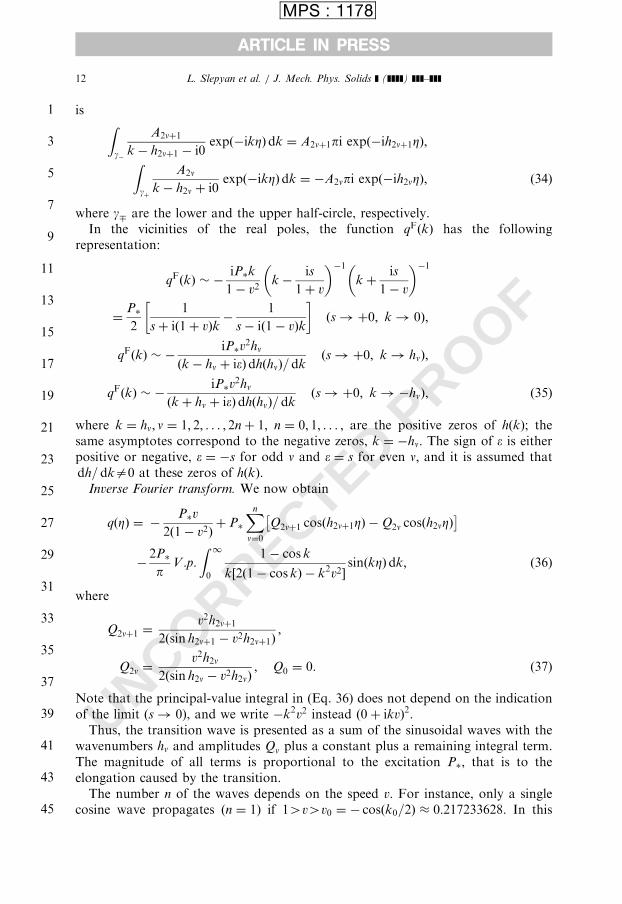
Inverse Fourier transform. We now obtain

qðZÞ ¼ �P�v

2ð1� v2Þþ P�

Xn

n¼0

Q2nþ1 cosðh2nþ1ZÞ � Q2n cosðh2nZÞ� �

�2P�

pV :p:

Z 1

0

1� cos k

k½2ð1� cos kÞ � k2v2�sinðkZÞdk; ð36Þ

where

Q2nþ1 ¼v2h2nþ1

2ðsin h2nþ1 � v2h2nþ1Þ;

Q2n ¼v2h2n

2ðsin h2n � v2h2nÞ; Q0 ¼ 0: ð37Þ

Note that the principal-value integral in (Eq. 36) does not depend on the indicationof the limit (s ! 0), and we write �k2v2 instead ð0þ ikvÞ2:

Thus, the transition wave is presented as a sum of the sinusoidal waves with thewavenumbers hn and amplitudes Qn plus a constant plus a remaining integral term.The magnitude of all terms is proportional to the excitation P�; that is to theelongation caused by the transition.

The number n of the waves depends on the speed v: For instance, only a singlecosine wave propagates (n ¼ 1) if 14v4v0 ¼ � cosðk0=2Þ � 0:217233628: In this

1

3

5

7

9

11

13

15

17

19

21

23

25

27

29

31

33

35

37

39

41

43

45

ARTICLE IN PRESS

MPS : 1178


UNCORRECTED PROOF

case, k ¼ k0 � 8:986818915 because k0 is the first positive root of Eq. (22) or,equivalently, tan k=2 ¼ k=2:

Strain at the transition front and distant asymptotes. Note that the strain iscontinuous at Z ¼ 0: The inhomogeneous, Eq. (36), and the homogeneous, q0; partsof the solution give us in sum the expression for the total strain at Z ¼ 0 as

qtotalð0Þ ¼ q0 �P�v

2ð1� v2Þþ P�

Xn

n¼0

Q2nþ1 � Q2n

� : ð38Þ

From Eqs. (18), where qð0Þ means the total elongation, and from Eq. (38) we findthat

q0 ¼ q� þP�v

2ð1� v2Þ� P�

Xn

n¼0

Q2nþ1 � Q2n

� : ð39Þ

To find asymptotes for Z ! �1 we choose another way of the calculation of theinverse-transform integral. Deform the integration path from the real axis upwardfor Zo0 and downward for Z40 (to have the exponential multiplier vanished whenk ! �i1) without crossing the poles. In this way, the result is expressed as aninfinite set of the residues (but not the half-residues!); however, contributions of thepoles with nonzero imaginary parts vanish at Z ! �1; and only a finite number ofcontributions from the real poles remains. Referring to Eqs. (35) and (39) we get thefollowing.

The reflective uniform wave is

qref ¼P�

2ð1þ vÞðZo0Þ: ð40Þ

The uniform wave propagating ahead of the transition front is

qhead ¼ �P�

2ð1� vÞþ q0 ¼ q� �

P�

2ð1� v2Þ� P�

Xn

n¼0

Q2nþ1 � Q2n

� ðZ40Þ: ð41Þ

Asymptotes for the total elongations are

qtotalðZÞ � q� þP�

2ð1� v2Þ� P�

Xn

n¼0

Q2nþ1 � Q2n

�

þ 2P�

Xn

n¼0

Q2nþ1 cosðh2nþ1ZÞ ðZ ! �1Þ;

qtotalðZÞ � q� �P�

2ð1� v2Þ� P�

Xn

n¼0

Q2nþ1 � Q2n

�

� 2P�

Xn

n¼0

Q2n cosðh2nZÞ ðZ ! 1Þ: ð42Þ

Tensile force and particle velocity in the uniform waves. Further we find expressionsfor the tensile force and the particle velocity corresponding to the uniform (zerowavenumber) waves behind the transition front. It follows from Eqs. (39) and (40)

1

3

5

7

9

11

13

15

17

19

21

23

25

27

29

31

33

35

37

39

41

43

45

ARTICLE IN PRESS

MPS : 1178


UNCORRECTED PROOF

that the constant part of the tensile force in the second branch of the dependence forthe original problem is

T ¼ q0 þ qref � P� ¼ q� �1� 2v2

2ð1� v2ÞP� � P�

Xn

n¼0

Q2nþ1 � Q2n

� ðZo0Þ: ð43Þ

Computing the particle velocity we recall that there are two uniform waves behindthe transition front: one is the incident wave (with the strain q0) propagating to theright, and the other is the reflected wave caused by the transition; it propagates to theleft with the unit nondimensional speed. The nondimensional particle velocities inthe former and the latter are [see Eq. (20)]

du

dt¼ �q0 and

du

dt¼ qref ðZo0Þ; ð44Þ

respectively. The total uniform particle velocity is thus

du

dt¼

P�

2ð1þ vÞ� q0 ¼ �q� þ

1� 2v

2ð1� v2ÞP� þ P�

Xn

n¼0

Q2nþ1 � Q2n

� ðZo0Þ: ð45Þ

The nondimensional tensile force and particle velocities ahead of the transition frontare equal to the strain q and �q; respectively. Recall that the particle velocities arethe same for the original and equivalent problems.

Calculation of the speed v. The obtained solution depends on the speed v which isstill unknown. It can be determined using the condition at Z ! �1 ðm ¼ �NÞ asthe applied force P equal to the uniform part of the tensile force T ; or as a givenuniform part of the particle velocity �w: The corresponding relations follow fromEqs. (43) and (45) as

1� 2v2


Xn

n¼0

Q2nþ1 � Q2n

� ¼ q� �P;

1� 2v


Xn

n¼0

Q2nþ1 � Q2n

� ¼ q� � w: ð46Þ

It can be seen now that the solution depends only on the ratios

P0 ¼P

q�

; P0� ¼

P�

q�

; w0 ¼w

q�

; ð47Þ

but not on the parameters P;P� and w themselves.2 In these terms, the aboveequations become

2These ratios could be used of course as nondimensional values from the very beginning; however, we

introduce them only now to avoid a nonusual form of some relation for the waves.

1

3

5

7

9

11

13

15

17

19

21

23

25

27

29

31

33

35

37

39

41

43

45

ARTICLE IN PRESS

MPS : 1178


1� 2v2

2ð1� v2ÞP0� þ P0

�

Xn

n¼0

Q02nþ1 � Q0

2n

� ¼ 1�P0;

1� 2v

2ð1� v2ÞP0� þ P0

�

Xn

n¼0

Q02nþ1 � Q0

2n

� ¼ 1� w0: ð48Þ

Eqs. (48) serve for the determination of the transition wave speed v: They containtwo nondimensional parameters; parameter P0

� defines the material properties, andP0 or w0 describes the level of external excitation.

ROOF2.3. Discussion of the results

Dependencies (48) are shown in Fig. 5. We notice peaks in the dependence on thespeed v: These peaks (they are infinite) correspond to the resonant values of thetransition wave speed which cannot be achieved in the steady-state regime. For theresonant speed, the group and phase velocities coincide, that is, the ray o ¼ kv istangent to the dispersion curve oðkÞ ¼ 2j sin k=2jsign k; see case 3 in Fig. 4. When thephase velocity, i.e. the transition wave speed increases and approaches the resonantlevel, the two waves (with the wavenumbers tending to each other) coincide, see Fig.

UNCORRECTED P

0 0.1 0.2 0.3 0.4 0.5 0.6 0.7 0.8 0.9 10

0.1

0.2

0.3

0.4

0.5

0.6

0.7

0.8

0.9

1

v

P0

Fig. 5. The external action level versus the transition front speed: Nondimensional tension force P0 as a

function of the speed, v: The (infinite) peaks correspond to the resonant speeds where two zeros of hðkÞ

coincide, see Fig. 4.

1

3

5

7

9

11

13

15

17

19

21

23

25

27

29

31

33

35

37

39

41

43

45

ARTICLE IN PRESS

MPS : 1178


OF

4. In this way, the amplitudes of the waves increase unboundedly, and this is reflectedby the lifted graphs in Fig. 5. After the speed exceeds the resonance level the graphimmediately drops to a ‘regular’ level because the mentioned two waves are notexcited at the post-critical regime.

Note, that such infinite peaks exist only in the steady-state solution; they reflectthe discontinuity in the assumed constant-speed solution that depends on v as aparameter. There are no discontinuities in a time-dependent solution with anincreasing speed crossing the resonant level. In this transient case, the peak is finiteand it’s height depends on how fast the resonant level is passed. Therefore, the peaksare not insurmountable obstacles as they look in Fig. 5, and the wave speeds abovethe main resonance speed are not forbidden.

In fact, only the waves with these high speeds are realizable. Indeed, consideringwhether or not the transition occurs at Z ¼ 0 we have to check if the elongation atZ40 is below the critical level. This is the case in the high-speed region where theresistance monotonically grows with the speed. This phenomenon for the crackpropagation in a discrete lattice was noted and investigated by Marder and Gross(1995). Numerical results discussed below help to elucidate this point.

RO

UNCORRECTED P2.4. Energy relations

From Eqs. (43) and (45) it follows that in terms of the nondimensional values

w0 ¼ P0 þv

1þ vP0�: ð49Þ

The energy flux from Z ¼ �1 caused by the external force P0 is

N0 ¼ P0w0 ¼ P0 P0 þv

1þ vP0�

� �¼ w0 w0 �

v

1þ vP0�

� �: ð50Þ

This energy flux increases the strain and kinetic energies of the chain. A part ofthis energy corresponds to the ‘macrolevel’ chain dynamics, that is to the waveswhich are uniform in each region, Zo0 and Z40: The other part is carried awayfrom the transition front by the sinusoidal waves, see Eq. (36). This latter part can beconsidered as the dissipation (as a wave dissipation). The wave dissipation can becalculated as the difference between the energy flux (50) and the macrolevel energyflux in the uniform wave ahead of the transition front [the latter is equal to�qhead du= dt at Z40; see Eq. (41)].

There is a more straightforward way to calculate the dissipation per unit time.Consider the macrolevel energy release rate per unit length G0 equal to the differencebetween the work produced during the transition and the energy required for thetransition, see Fig. 6. Both ways lead to the same result:

PROOF

1

3

5

7

9

11

13

15

17

19

21

23

25

27

29

31

33

35

37

39

41

43

45

ARTICLE IN PRESS

MPS : 1178

P

q

0

0

q +

q +

1

1

T0

q -

Fig. 6. The nondimensional energy dissipation as the difference between the transition work and the

increase of the strain energy during the transition on the macrolevel. The former is defined by the

trapezium ðqþ; 0Þ; ðqþ; qþÞ; ðq�;P0Þ; ðq�; 0Þ; while the latter is numerically equal to the area under the

dependence within the segment qþ; q�:


UNCORRECTED D0 ¼ G0v ¼ ðG� UÞv;

G ¼1

2ðP0 þ qþÞðq� � qþÞ;

U ¼1

2ðq�Þ

2�

1

2ðqþÞ

2� P0

�ðq� � 1Þ;

qþ ¼ P0 �v2

1� v2P0�;

q� ¼ P0 þ P0�: ð51Þ

Here the nondimensional values are used in accordance with Eq. (47); G is thetransition work per unit length, U is the strain energy increase due to the transition,q� are the uniform parts of the nondimensional strain, divided by q�; for Z40 andZo0; respectively[see Eqs. (39)–(41)].

From system Eqs. (51) we compute

D0 ¼1� 2v2

2ð1� v2ÞP0� þP0 � 1

� �P0�v: ð52Þ

In terms of dimensional variables, the wave dissipation can be rewritten as

D̂ ¼1� 2v2=c2

2ð1� v2=c2ÞP� þP0 � mq�

� �P�v

ma: ð53Þ

The Maxwell dissipation-free transition would correspond to zero wave

1

3

5

7

9

11

13

15

17

19

21

23

25

27

29

31

33

35

37

39

41

43

45

ARTICLE IN PRESS

MPS : 1178


OOF

dissipation or to the relation

1� 2v2

2ð1� v2ÞP0� þP0 � 1 ¼ 0: ð54Þ

In this hypothetic case, the transition line on the dependence crosses the jumpvertical segment at the middle as shown in Fig. 6. Because of the wave dissipation,the transition occurs at larger values.

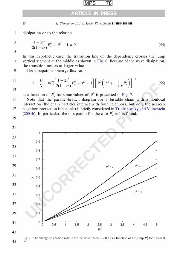
The dissipation – energy flux ratio

l ¼D

N¼ vP0

�

1� 2v2

2ð1� v2ÞP0� þP0 � 1

� �P0 P0 þ

v

1þ vP0�

� �� 1

ð55Þ

as a function of P0� for some values of P0 is presented in Fig. 7.

Note that the parallel-branch diagram for a bistable chain with a nonlocalinteraction (the chain particles interact with four neighbors, but only the nearest-neighbor interaction is bistable) is briefly considered in Truskinovsky and Vainchtein(2004b). In particular, the dissipation for the case P0

� ¼ 1 is found.

UNCORRECTED PR

0 0.5 1 1.5 2 2.5 3 3.5 4 4.5 50

0.1

0.2

0.3

0.4

0.5

0.6

0.7

0.8

0.9

1

P0*

λ

P0 = 2 P0 = 3

P0 = 4

Fig. 7. The energy dissipation ratio l for the wave speed v ¼ 0:5 as a function of the jump P0� for different

P0:

1

3

5

7

9

11

13

15

17

19

21

23

25

27

29

31

33

35

37

39

41

43

45

ARTICLE IN PRESS

MPS : 1178


2.5. Transient regimes

A finite chain consisting of 32 cells was examined numerically. Point m ¼ 0 wasfixed, while the end particle, m ¼ 32; was the subject of an impact. The resultspresented in Fig. 8 correspond to the dynamics of the initially unstressed restingchain with P0

� ¼ 1: For t40 the chain is under a given constant velocity of the endparticle. In particular, this case was examined to compare the speeds of the transitionfront derived analytically from Eq. (48) and computed numerically. A goodagreement between the analytical and numerical results was found. This is alsoshown in Fig. 9 where the numerical results are marked by asterisks. Dynamicbehavior of the chain under an inelastic impact of the end particle by a rigid mass is

UNCORRECTED PROOF

0 2.5 10 20 30 3840 50 600

(a) (b)

(c)

1.55

10

15

20

25

30

35

40

45

50Trajectories: w0=0.3 Trajectories: w0=0.5

Trajectories: w0=0.7

0 2.5 10 20 30 34.75 40 50 6001.5

10

20

30

40

50

60

70

5 7.710 15 20 25 30 33.6 40 45 5001

5

10

15

20

25

30

35

40

45

Fig. 8. Position of the knots versus time for a 32-cell chain under a given velocity, w0; of the end particle:

(a) w0 ¼ 0:3; (b) w0 ¼ 0:5; (c) w0 ¼ 0:7: The chain with the jump discontinuity of the dependence P0� ¼ 1 is

initially unstressed and unmoving. For t40 the chain is under a given constant velocity of the end particle.

A weak elastic wave propagates with the unit (nondimensional) speed; the transition front is marked by an

inclined straight line, its speed numerically evaluated from the graph is shown by asterisks in Fig. 9 in

comparison with the results of analytical calculation using Eq. (23). The elastic wave reflection off the fixed

point seen in the graphs can cause an opposite transition wave.

D PROOF

1

3

5

7

9

11

13

15

17

19

21

23

25

27

29

31

33

35

37

39

41

43

45

ARTICLE IN PRESS

MPS : 1178

0.2 0.3 0.4 0.5 0.6 0.7 0.8 0.9 10

0.1

0.2

0.3

0.4

0.5

0.6

0.7

0.8

0.9

V

xx

x

x

x

x

x

P0

Fig. 9. Speed of the transition front analytically calculated using Eq. (23). Numerically evaluated

transition wave speed is shown by asterisks.


TEpresented in Fig. 10. This case corresponds to the conditions of an initial speedw0 ¼ du32ð0Þ=dt of an increased end mass M0

X1:
C
UNCORRE3. Waves of transition: nonparallel branches

3.1. Formulation and solution

We now consider a general case of the constitutive relation assuming that thebranches of the force–elongation diagram also differ by the modules:

T ¼q if tot�;

gq � P�� if t4t�:

(ð56Þ

We use here the nondimensional values; t� is the instance of the transition. Thedistance from the first branch to the other at q ¼ 0; P��; is expressed through thejump, P�; and the critical elongation, q�; as (see Fig. 2(c))

P�� ¼ P� � ð1� gÞq�: ð57Þ

The parallel-branch case considered above corresponds to g ¼ 1:

RECTED PROOF

1

3

5

7

9

11

13

15

17

19

21

23

25

27

29

31

33

35

37

39

41

43

45

ARTICLE IN PRESS

MPS : 1178

0(a) (b)

(c)

10 20 30 40 50 60 70 80 90 1000

5

10

15

20

25

30

35

40

45M0 = 2, w0 = 2

0 10 20 30 40 50 60 70 80 90 1000

10

20

30

40

50

60

10 20 30 40 50 60 70 80 90 1000

10

20

30

40

50

60

70

M0 = 5, w0 = 4

M0 = 5, w0 = 2

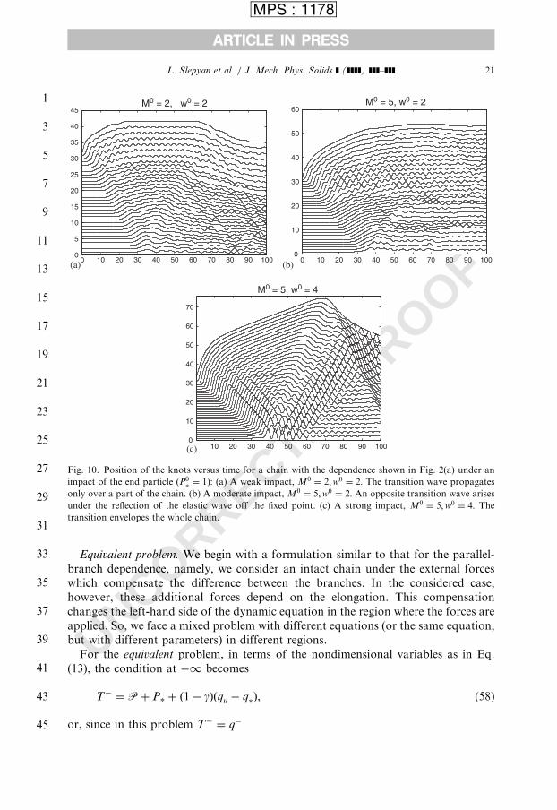
Fig. 10. Position of the knots versus time for a chain with the dependence shown in Fig. 2(a) under an

impact of the end particle (P0� ¼ 1): (a) A weak impact, M0 ¼ 2;w0 ¼ 2: The transition wave propagates

only over a part of the chain. (b) A moderate impact, M0 ¼ 5;w0 ¼ 2: An opposite transition wave arises

under the reflection of the elastic wave off the fixed point. (c) A strong impact, M0 ¼ 5;w0 ¼ 4: Thetransition envelopes the whole chain.


UNCOREquivalent problem. We begin with a formulation similar to that for the parallel-branch dependence, namely, we consider an intact chain under the external forceswhich compensate the difference between the branches. In the considered case,however, these additional forces depend on the elongation. This compensationchanges the left-hand side of the dynamic equation in the region where the forces areapplied. So, we face a mixed problem with different equations (or the same equation,but with different parameters) in different regions.

For the equivalent problem, in terms of the nondimensional variables as in Eq.(13), the condition at �1 becomes

T� ¼ Pþ P� þ ð1� gÞðqu � q�Þ; ð58Þ

or, since in this problem T� ¼ q�

1

3

5

7

9

11

13

15

17

19

21

23

25

27

29

31

33

35

37

39

41

43

45

ARTICLE IN PRESS

MPS : 1178


UNCORRECTED PROOF

q� ¼1

g½Pþ P� � ð1� gÞq�� ðZ ¼ �1Þ; ð59Þ

where the superscript ‘�’ is used to indicate the uniform parts of the values at Zo0:The equation for the transition wave that propagates with a constant speed becomes

d2um

dt2¼ qmþ1ðtÞ � qmðtÞ þ PðZÞHð�ZÞ � PðZþ 1ÞHð�Z� 1Þ; ð60Þ

where

PðZÞ ¼ P� þ ð1� gÞðq � q�Þ; ð61Þ

Z ¼ m � vt; and it is assumed that 0ovominðffiffiffig

p; 1Þ:

As in the previous case, for g ¼ 1; we represent the solution as the sum of anincident wave, q0 = const, and a steady-state solution with respect to the particlevelocity and elongation qðZÞ induced by the forces PðZÞ

q ¼ qtotal ¼ q0 þ qðZÞ: ð62Þ

Eqs. (60) and (61) can now be rewritten in the form

v2d2qðZÞdZ2

þ 2qðZÞ � qðZþ 1Þ � qðZ� 1Þ

¼ ½P� � ð1� gÞðq� � q0Þ�½2Hð�ZÞ � Hð�Zþ 1Þ � Hð�Z� 1Þ�

þ ð1� gÞ½2qðZÞHð�ZÞ � qðZ� 1ÞHð�Zþ 1Þ � qðZþ 1ÞHð�Z� 1Þ�;

PðZÞ ¼ P� þ ð1� gÞðqðZÞ þ q0 � q�Þ: ð63Þ

Fourier transform. The Fourier transform of the equation leads to

hðkÞqþðkÞ þ gðkÞq�ðkÞ ¼ ½P� � ð1� gÞðq� � q0Þ�2ð1� cos kÞ

ik; ð64Þ

where

hðkÞ ¼ ðs þ ikvÞ2 þ 2ð1� cos kÞ;

gðkÞ ¼ ðs þ ikvÞ2 þ 2gð1� cos kÞ ð65Þ

and s ! þ0 (here we consider the prelimiting expression s þ ikv instead ikv inaccordance with the above-mentioned causality principle). Further, qþðkÞ and q�ðkÞ

are the right-side and left-side Fourier transforms

qþðkÞ ¼

Z 1

0

qðZÞeikZ dZ;

q�ðkÞ ¼

Z 0

�1

qðZÞeikZ dZ: ð66Þ

It follows from Eq. (65) that

2ð1� cos kÞ ¼hðkÞ � gðkÞ

1� g: ð67Þ

1

3

5

7

9

11

13

15

17

19

21

23

25

27

29

31

33

35

37

39

41

43

45

ARTICLE IN PRESS

MPS : 1178


UNCORRECTED PROOF

Substitute this into Eq. (64), and rewrite it as

LðkÞqþðkÞ þ q�ðkÞ ¼q��

ik½LðkÞ � 1�; ð68Þ

where

LðkÞ ¼hðkÞ

gðkÞ;

q�� ¼P� � ð1� gÞðq� � q0Þ

1� g: ð69Þ

Note that the function LðkÞ is estimated as LðkÞ � 1 ¼ O(k2) (k ! 0) and hence theright-hand side of Eq. (68) is regular at k ¼ 0:

Factorization of LðkÞ: To find two functions q�ðkÞ from the single equation (68) weuse the Wiener–Hopf technique. The first step is the factorization of LðkÞ: It shouldbe represented as the product

LðkÞ ¼ LþðkÞL�ðkÞ; ð70Þ

where LþðkÞ has no zeros and singularities in the upper complex half-plane includingthe real axis, and L�ðkÞ has no zeros and singularities in the lower half-planeincluding the real axis. The factorization can be done (for s40) using the Cauchy-type integral.

Before this we normalize LðkÞ with the goal to separate its zeros and poles in avicinity of k ¼ 0: Represent LðkÞ as

LðkÞ ¼ L0ðkÞlðkÞ; ð71Þ

where

lðkÞ ¼½s þ ið1þ vÞk�½s � ið1� vÞk�

½s þ iðffiffiffig

pþ vÞk�½s � ið

ffiffiffig

p� vÞk�

g� v2

1� v2: ð72Þ

Note that

Lð0Þ ¼ 1; lð0Þ ¼g� v2

1� v2; L0ð0Þ ¼

1� v2

g� v2;

Lð�1Þ ¼ lð�1Þ ¼ L0ð�1Þ ¼ 1: ð73Þ

In addition, the index of each of the considered functions is equal to zero, forexample

IndL0ðkÞ ¼1

2p½ArgL0ð1Þ �ArgL0ð�1Þ� ¼ 0: ð74Þ

Factorization of the multiplier lðkÞ is straightforward:

1

3

5

7

9

11

13

15

17

19

21

23

25

27

29

31

33

35

37

39

41

43

45

ARTICLE IN PRESS

MPS : 1178


UNCORRECTED PROOF

lðkÞ ¼ lþðkÞl�ðkÞ;

lþðkÞ ¼s � ið1� vÞk

s � iðffiffiffig

p� vÞk

ffiffiffiffiffiffiffiffiffiffiffiffiffig� v2

1� v2

r;

l�ðkÞ ¼s þ ið1þ vÞk

s þ iðffiffiffig

pþ vÞk


1� v2

r: ð75Þ

The functions L0ðkÞ and lnL0ðkÞ are regular in a vicinity of k ¼ 0: The conditions atinfinity in Eqs. (73) and the equality in Eq. (74) allows us to use the Cauchy-typeintegral for the factorization of L0ðkÞ:

L0ðkÞ ¼ L0þðkÞL

0�ðkÞ;

L0�ðkÞ ¼ exp �

1

2pi

Z 1

�1

lnL0ðxÞx� k

dx� �

½ArgLð1Þ ¼ 0�; ð76Þ

where Ik40 for Lþ and Iko0 for L�:We mention in addition, that when s ¼ 0 there are real singular points of lnL0ðkÞ;

that correspond to the real zeros and singular points of L0ðkÞ and, therefore, of LðkÞ:When s40; these singularities move either to the upper or the lower half-plane.Thus, for s40 functions L0ðkÞ and 1=L0ðkÞ are regular on the real axis; functionsL0þðkÞ and 1=L0

þðkÞ are regular at the half-plane IkX0; functions L0�ðkÞ and 1=L0

�ðkÞ

are regular at the half-plane Ikp0: When s ! 0; Arg L0ðkÞ (in contrast to Arg LðkÞ)uniformly tends to zero in a vicinity of the origin, k ¼ 0 (Arg L0ð0Þ=Arg Lð0Þ ¼ 0).Function Arg L0ðkÞ is odd, while ln jL0ðkÞj is even.

Using these facts, we derive from Eq. (76) and (75) the following representations:

L0�ð0Þ ¼ lim

p!þ0L0ð�ipÞ ¼

ffiffiffiffiffiffiffiffiffiffiffiffiffi1� v2

g� v2

sR�1;

L0�ð�1Þ ¼ 1;

LþðkÞ �s � ið1� vÞk

s � iðffiffiffig

p� vÞk

R ðk ! 0Þ;

L�ðkÞ �s þ ið1þ vÞk

s þ iðffiffiffig

pþ vÞk

1

Rðk ! 0Þ;

L�ð0Þ ¼ R�1; R ¼ exp1

p

Z 1

0

ArgL0ðxÞx

dx� �

;

L�ð�i1Þ ¼ l�ð�1Þ ¼ðffiffiffig

pþ vÞð1� vÞ

ðffiffiffig

p� vÞð1þ vÞ

� ��1=2

: ð77Þ

Here, the first multiplier in the expression for L0�ð0Þ is defined by a half-residue at

k ¼ 0:Assume that s ¼ þ0 and let us number the increasing positive zeros of hðkÞ as

h1oh2o � � �oh2lþ1 and similarly, the increasing positive zeros of gðkÞ asg1og2o � � �og2dþ1: The transition front speed, v; is assumed such that the zeros

1

3

5

7

9

11

13

15

17

19

21

23

25

27

29

31

33

35

37

39

41

43

45

ARTICLE IN PRESS

MPS : 1178


UNCORRECTED PROOF

are simple (of the first order) and the corresponding functions change their signswhen they pass the root.

From expressions (65), we determine arguments of hðkÞ and gðkÞ:

Arg hðkÞ ¼ 0 ðh2nokoh2nþ1Þ; Arg hðkÞ ¼ p ðh2nþ1okoh2nþ2Þ;

n ¼ 0; 1; . . . ; l; h0 ¼ 0; h2lþ2 ¼ 1;

Arg gðkÞ ¼ 0 ðg2nokog2nþ1Þ; Arg gðkÞ ¼ p ðg2nþ1okog2nþ2Þ;

n ¼ 0; 1; . . . ; d; g0 ¼ 0; g2dþ2 ¼ 1: ð78Þ

Finally, function R can thus be expressed in terms of the real zeros of hðkÞ and gðkÞ

as

R ¼h2h4:::h2l g1g3:::g2dþ1

h1h3:::h2lþ1 g2g4:::g2d

: ð79Þ

Wiener–Hopf equation. The Wiener–Hopf equation (68) can now be written as

LþðkÞqþðkÞ þq�ðkÞ

L�ðkÞ¼

q��

ikLþðkÞ �

1

L�ðkÞ

� �; ð80Þ

where k ¼ 0 is still a regular point of the right-hand side. Next we rewrite thisequation in the identical form

LþðkÞqþðkÞ þq�ðkÞ

L�ðkÞ¼ q��

LþðkÞ �R

ik�

1

L�ðkÞ�R

� �1

ik

�; ð81Þ

where k ¼ 0 is a regular point for both terms on the right-hand side.Solution. We now obtain the solution to Eq. (81) as

qþðkÞ ¼q��

ik1�

R

LþðkÞ

� �;

q�ðkÞ ¼ �q��

ik1�RL�ðkÞ½ �: ð82Þ

In particular, we find from these formulas and from Eqs. (77), the followingrepresentations:

qð0Þ ¼ q0 þ limk!i1

ð�ikÞ½qþðkÞ ¼ q0 þ limk!�i1

ðikÞq�ðkÞ

¼ q0 � q��ð1�R�Þ ¼ R�q0 � ð1�R�ÞP�

1� g� q�

� �;

R� ¼ R

ffiffiffiffiffiffiffiffiffiffiffiffiffiffiffiffiffiffiffiffiffiffiffiffiffiffiffiffiffiffiffiðffiffiffig

p� vÞð1þ vÞ

ðffiffiffig

pþ vÞð1� vÞ

s: ð83Þ

Using condition (18) of the transition we now find the incident wave as

q0 ¼ q� þP�

1� g1

R�

� 1

� �: ð84Þ

The uniform part of the strain, as the contribution of singular points approachingzero with s ! 0; is

1

3

5

7

9

11

13

15

17

19

21

23

25

27

29

31

33

35

37

39

41

43

45

ARTICLE IN PRESS

MPS : 1178


UNCORRECTED PROOF

q ¼ qþ ¼ q0 �q��ð1�

ffiffiffig

pÞ

1� v¼ q� �

P�

1� g1�


1� v2

r1

R

!ðZ40Þ;

q ¼ q� ¼ q0 þq��ð1�

ffiffiffig

pÞffiffiffi

gp

þ v¼ q� �

P�

1� g1�


g� v2

s1

R

!ðZo0Þ: ð85Þ

At Z40 the corresponding nondimensional particle velocity, by its value, is equalto �q since it corresponds to a free wave propagating to the right with the unit speed.To find the uniform part of the particle velocity at Zo0 we use the momentumconservation law for the original problem where there are no external forces at Zo0

du

dt

� ��

�du

dt

� �þ

¼ �1

vT� � Tþ�

ð86Þ

with

Tþ ¼ qþ ðZ40Þ;

T� ¼ q� � P� � ð1� gÞðq� � q�Þ ðZo0Þ; ð87Þ

where the superscripts � are used to indicate the uniform parts of the values at Z40and Zo0; respectively. As a result we find

du

dt

� �þ

¼ �q� þP�

1� g1�


1� v2

r1

R

!;

du

dt

� ��

¼du

dt

� �þ

�P�v

Rffiffiffiffiffiffiffiffiffiffiffiffiffiffiffiffiffiffiffiffiffiffiffiffiffiffiffiffiffiffiffiðg� v2Þð1� v2Þ

p¼ �q� �

P�

1� g


g� v2

sgþ v

1þ v

1

R� 1

!: ð88Þ

The limit at g ¼ 1: To find the limits of the uniform strains (85) and particlevelocities (88) we first have to find the corresponding asymptote of R: If g ! 1 thengn ! hn and

gðgnÞ ¼ hðgnÞ � ð1� gÞ2ð1� cos gnÞ ¼ 0;

dhðhnÞ

dkðgn � hnÞ � 2ð1� gÞð1� cos hnÞ;

gn

hn� 1þ

ð1� gÞhnv2

2ðsin hn � hnv2Þð89Þ

and referring to Eq. (79)

1

R� 1� ð1� gÞ

Xn

n¼0

Q2nþ1 � Q2n

� : ð90Þ

It can now be seen that in the limit, g ! 1; expressions (85) and (88) lead to those forthe parallel-branch cases (42) and (45).

1

3

5

7

9

11

13

15

17

19

21

23

25

27

29

31

33

35

37

39

41

43

45

ARTICLE IN PRESS

MPS : 1178


The force–speed relation. Relations between the speed, v; and the applied force, P;or the speed and a given particle velocity, �w; follows from Eqs. (87), (85) and (88)as

P�

1� g


g� v2

sgR

� 1

!¼ P� q�;

P�

1� g


g� v2

sgþ v

1þ v

1

R� 1

!¼ w � q�: ð91Þ

The nondimensional values (47) can now be used to decrease the number ofparameters in these equations. Recall that this is achieved by means of division by q�:The P��v relations for P� ¼ q�; g ¼

12 and g ¼ 2 are presented in Fig. 11.

UNCORRECTED PROOF

0

1

2

3

4

R

0.2 0.4 0.6 0.8 1V

Fig. 11. The force–speed dependence for P� ¼ mq�: Here V ¼ v=c and R ¼ P=P�: The lower curve (R ¼ 2

at V ¼ 1) corresponds to g ¼ 2; the upper curve (R ! 1 when V !ffiffiffi5

p) corresponds to g ¼ 1

2:

1

3

5

7

9

11

13

15

17

19

21

23

25

27

29

31

33

35

37

39

41

43

45

ARTICLE IN PRESS

MPS : 1178


TED PROOF

3.2. Sinusoidal waves and dissipation

As follows from the solution in Eq. (82) the oscillating waves corresponding towavenumbers h2n carry energy from the transition front to þ1 since the groupvelocity at k ¼ h2n is greater than the phase velocity v: The waves corresponding towavenumbers g2nþ1 carry energy to �1; these waves are present behind thetransition front because they correspond to the opposite relation between the groupand phase velocities, see Fig. 4. The amplitudes of the sinusoidal waves can bedetermined in the same way as in the case P� ¼ ð1� gÞq� considered in Slepyan andTroyankina, 1984 (also see Slepyan, 2002) using a different type of the factorization.The total dissipation due to the existence of the oscillating waves can be calculated asin the considered above parallel-branch case using the dependence presented in Fig.2(c). The energy dissipation rate per unit time is

D ¼v

2½ðT� þ TþÞðq� � qþÞ � ðqþ þ q�Þðq� � qþÞ

� ðq� � P� þ T�Þðq� � q�Þ�: ð92Þ

Recall the values with the upper sign � correspond to the uniform parts of those atZ40 and Zo0; respectively. Using the obtained above expressions for the values inEq. (92) it can be found that

D ¼P2�v

2ð1� gÞ1

R2� 1

� �: ð93Þ

At the same time, the total energy flux is

N ¼ T�w: ð94Þ

C

UNCORRE4. Conclusions

1. In this paper, especially in Part I, it is demonstrated that a properly designedbistable structure being under an impact can absorb an increased amount of energy.This is achieved by means of the large strain delocalization and by the transfer of aconsiderable part of the input energy (for example, the kinetic energy of thehammering mass) into the energy of high-frequency oscillations. The bistablestructure role is just the delocalization and transformation of the nonoscillating waveenergy into the oscillating one. In Part I of the paper, the stress–strain dependencewith a gap between two branches of the resistance is considered. Generalconsiderations, numerical simulations and analytical estimations are presented forquasi-static and dynamic extension of the chain to elucidate the role of the bistabilityand especially the role of the gap in the energy consumption; an optimal value of thegap is found. In Part II, the same bistable-bond chain is considered, but without thegap. This simplification allowed us to obtain analytical solutions for an arbitrary

1

3

5

7

9

11

13

15

17

19

21

23

25

27

29

31

33

35

37

39

41

43

45

ARTICLE IN PRESS

MPS : 1178


CTED PROOF

relation between the branch modules. The analytical treatment of the problemrepresents the main contents of this Part.

2. For the energy consumption in an elastic bistable structure the constraint is thatthe strength of the second branch, Tðq�� 0Þ; must be large enough to withstand thedynamic overshoot caused by the sudden breaks of the basic links, that is, thewaiting links must withstand both the nonoscillating and oscillating waves. Note,however, that the overshoot can be suppressed by internal inelastic resistances whichspeed up the energy transfer from the mechanical oscillations to heat (see Slepyan,2000, 2002). In this sense, the nonoscillating wave amplitudes are critical, and theenergy transfer to the oscillating waves that decreases the nonoscillating waveamplitudes is fruitful.

3. Mathematically, two cases are different: parallel-branch diagram, g ¼ 1; andnonparallel one, ga1: Although the former follows from the latter as a limit, themathematical difference reflects different physics. In the parallel-branch case, thereexist pure resonances which correspond to a hypothetic situation where thetransition front speed and hence the wave phase velocity coincide with the groupvelocity. In this case, there is no energy flux (for this resonant wave) from thetransition front, and the wave amplitude increases in time. The steady-state solutiondoes not exist at this speed. In contrast, in the case of different modules, if the speedcorresponds to a resonant wave for a one branch, it does not correspond to such awave for the other, and the latter represents a nonresonant waveguide for the energy.As a result, there is no pure resonance speeds in this nonparallel case.

4. In this paper, a mechanical problem is considered, mainly as how the bistabilityincreases the energy consumption in the chain. At the same time, the formulationsand the results may have an interest in different fields, in particular, we can notewaves of instability or crushing waves in an extended structure, or a material phasetransition where the bistability or multistability plays a crucial role. In this Part, werefer to some phase transition papers where this model is exploited.
E
RR5. Uncited references

Charlotte and Truskinovsky (2002); Kresse and Truskinovsky (2003, 2004).
O NCAcknowledgements
This research was supported by The Israel Science Foundation, Grants No. 28/00-3 and No. 1155/04, ARO Grant No. 41363-MA, and NSF Grant No. DMS-0072717.
U References
Balk, A.M., Cherkaev, A.V., Slepyan, L.I., 2001a. Dynamics of chains with non-monotone stress–strain

relations. I. Model and numerical experiments. J. Mech. Phys. Solids 49, 131–148.

1

3

5

7

9

11

13

15

17

19

21

23

25

27

29

31

33

35

ARTICLE IN PRESS

MPS : 1178


ORRECTED PROOF

Balk, A.M., Cherkaev, A.V., Slepyan, L.I., 2001b. Dynamics of chains with non-monotone stress–strain

relations. II. Nonlinear waves and waves of phase transition. J. Mech. Phys. Solids 49, 149–171.

Bolotovsky, B.M., Stolyarov, S.N., 1972. On radiation principles for a medium with dispersion. In:

Problems for Theoretical Physics. Nauka, Moscow, pp. 267–280 (in Russian).

Charlotte, M., Truskinovsky, L., 2002. Linear chains with a hyper-pre-stress. J. Mech. Phys. Solids 50,

217–251.

Fedelich, B., Zanzotto, G., 1992. Hysteresis in discrete systems of possibly interacting elements with a

double-well energy. J. Nonlinear Sci. 2, 319–342.

Frenkel, J., Kontorova, T., 1938. On the theory of plastic deformation and twinning. Sov. Phys. JETP 13,

1–10.

Kresse, O., Truskinovsky, L., 2003. Mobility of lattice defects: discrete and continuum approaches. J.

Mech. Phys. Solids 51 (7), 1305–1332.

Kresse, O., Truskinovsky, L., 2004. Lattice friction for crystalline defects: from dislocations to cracks,

submitted for publication.

Marder, M., Gross, S., 1995. Origin of crack tip instabilities. J. Mech. Phys. Solids 43, 1–48.

Muller, I., Villaggio, P., 1977. A model for an elastoplastic body. Arch. Rat. Mech. Anal. 65, 25–46.

Ngan, S.-C., Truskinovsky, L., 1999. Thermal trapping and kinetics of martensitic phase boundaries. J.

Mech. Phys. Solids 47, 141–172.

Ngan, S.-C., Truskinovsky, L., 2002. Thermo-elastic aspects of dynamic nucleation. J. Mech. Phys. Solids

50, 1193–1229.

Puglisi, G., Truskinovsky, L., 2000. Mechanics of a discrete chain with bi-stable elements. J. Mech. Phys.

Solids 48, 1–27.

Puglisi, G., Truskinovsky, L., 2002a. Rate-independent hysteresis in a bi-stable chain. J. Mech. Phys.

Solids 50, 165–187.

Puglisi, G., Truskinovsky, L., 2002b. A model of transformational plasticity. Cont. Mech. Therm. 14,

437–457.

Rogers, R.C., Truskinovsky, L., 1997. Discretization and hysteresis. Physica B 233, 370–375.

Slepyan, L.I., 2000. Dynamic factor in impact, phase transition and fracture. J. Mech. Phys. Solids 48,

931–964.

Slepyan, L.I., 2001. Feeding and dissipative waves in fracture and phase transition. II. Phase-transition

waves. J. Mech. Phys. Solids 49, 513–550.

Slepyan, L.I., 2002. Models and Phenomena in Fracture Mechanics. Springer, Berlin.

Slepyan, L.I., Troyankina, L.V., 1984. Fracture wave in a chain structure. J. Appl. Mech. Techn. Phys. 25

(6), 921–927.

Slepyan, L.I., Troyankina, L.V., 1988. Impact waves in a nonlinear chain. In: Strength and Visco-

plasticity. Nauka, Moscow, pp. 301–305 (in Russian).

Truskinovsky, L., Vainchtein, A., 2004a. The origin of the nucleation peak in transformational plasticity.

J. Mech. Phys. Solids 52, 1421–1446.

Truskinovsky, L., Vainchtein, A., 2004b. Explicit kinetic relation from ‘‘first principles’’. In: Ogden, R.,

Gao, D. (Eds.), Mechanics of Material forces, Euromech 445, Advances in Mechanics and

Mathematics. Kluwer, Dordrecht, pp. 1–8 (in press).

UNC

Documents

Transition waves in bistable structures. II. Analytical