Transition State Clustering: UnsupervisedSurgical Trajectory Segmentation For RobotLearning

Sanjay Krishnan*1, Animesh Garg*2, Sachin Patil1, Colin Lea3, Gregory Hager3,Pieter Abbeel1, Ken Goldberg1,2 *denotes equal contribution

Abstract Over 500,000 Robot-Assisted Minimally-Invasive Surgeries were per-formed in 2014 [11]. There is a large and growing corpus of kinematic and videorecordings that have potential to facilitate human training and the automation ofsubtasks. A key step is to segment these multi-modal trajectories into meaningfulcontiguous sections in the presence of significant variations in spatial and tempo-ral motion, noise, and looping (repetitive attempts). Manual segmentation is proneto error and impractical for large datasets. We propose Transition State Clustering(TSC), which segments a set of surgical trajectories by detecting and clustering tran-sitions between linear dynamic regimes. TSC aggregates transition states from alldemonstrations into clusters using a hierarchical Dirichlet Process Gaussian MixtureModel in two phases, first over states and then temporally. After a series of mergingand pruning steps, the algorithm adaptively optimizes the number of segments, andthis process gives TSC additional robustness in comparison to other Gaussian Mix-ture Models (GMMs) algorithms. In a synthetic case study with two linear dynami-cal regimes, when demonstrations are corrupted with noise and temporal variations,TSC finds up to a 20% more accurate segmentation than GMM-based alternatives.On 67 recordings of surgical needle passing and suturing tasks from the JIGSAWSsurgical training dataset [8], supplemented with manually annotated visual features,TSC finds 83% of needle passing segments and 73% of the suturing segments foundby human experts.

1 IntroductionKinematic and fixed-camera video recordings from robot-assisted minimally inva-sive procedures (RMIS) are used in a number of applications such as surgical skillassessment [8], development of finite state machines for automation [12, 24], learn-ing from demonstration (LfD) [28], and calibration [21]. However, even in a con-sistent environment (e.g., on identical tissue phantoms), leveraging the raw data ischallenging. Surgical tasks are often multi-step procedures that have complex inter-actions with the environment, and as a result, demonstrations can vary widely.

One approach is segmentation of a trajectory by grouping states in locally similarsegments. Existing segmentation work in robotic surgery considers the supervised

1 EECS, 2IEOR, UC Berkeley, e-mail: sanjaykrishnan,animesh.garg,sachinpatil,pabbeel,goldberg@berkeley.edu3 Computer Science Department, The Johns Hopkins University, e-mail: clea1@jhu.edu,hager@cs.jhu.edu

1

2 Krishnan, Garg et al.

N Demonstrations

DP-GMM

Transition States Pruning &

Compaction

State DP-

GMM

Time DP-

GMM

M TS Clusters

TS Clusters

ρ, δ

Transition State Clustering

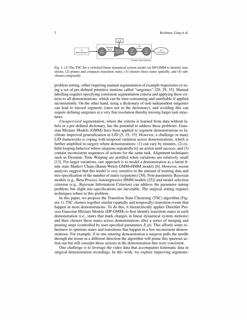
Fig. 1: (1) The TSC fits a switched linear dynamical system model via DP-GMM to identify tran-sitions, (2) prunes and compacts transition states, (3) clusters these states spatially, and (4) sub-clusters temporally.

problem setting, either requiring manual segmentation of example trajectories or us-ing a set of pre-defined primitive motions called “surgemes” [20, 29, 35]. Manuallabelling requires specifying consistent segmentation criteria and applying these cri-teria to all demonstrations, which can be time-consuming and unreliable if appliedinconsistently. On the other hand, using a dictionary of task-independent surgemescan lead to missed segments (ones not in the dictionary), and avoiding this canrequire defining surgemes at a very fine resolution thereby missing larger task struc-tures.

Unsupervised segmentation, where the criteria is learned from data without la-bels or a pre-defined dictionary, has the potential to address these problems. Gaus-sian Mixture Models (GMM) have been applied to segment demonstrations to fa-cilitate improved generalization in LfD [5, 19, 15]. However, a challenge in manyLfD frameworks is coping with temporal variation across demonstrations, which isfurther amplified in surgery where demonstrations: (1) can vary by minutes, (2) ex-hibit looping behavior where surgeons repeatedly try an action until success, and (3)contain inconsistent sequences of actions for the same task. Alignment techniquessuch as Dynamic Time Warping are justified when variations are relatively small[13]. For larger variations, one approach is to model a demonstration as a latent fi-nite state Markov Chain (Baum-Welch GMM+HMM model) [6]. However, recentanalyses suggest that this model is very sensitive to the amount of training data andmis-specification of the number of states (segments) [30]. Non-parametric Bayesianmodels (e.g., Beta-Process Autoregressive HMM models [25]) and model selectioncriterion (e.g., Bayesian Information Criterion) can address the parameter tuningproblem, but slight mis-specifications are inevitable. The surgical setting requirestechniques robust to this problem.

In this paper, we propose the Transition State Clustering (TSC) algorithm (Fig-ure 1). TSC clusters together similar (spatially and temporally) transition events thathappen in most demonstrations. To do this, it hierarchically applies Dirichlet Pro-cess Gaussian Mixture Models (DP-GMM) to first identify transition states in eachdemonstration (i.e., states that mark changes in linear dynamical system motions)and then clusters these states across demonstrations after a series of merging andpruning steps (controlled by user-specified parameters δ ,ρ). This affords some ro-bustness to spurious states and transitions that happen in a few inconsistent demon-strations. For example, if in one suturing demonstration a surgeon pulls the needlethrough the tissue in a different direction the algorithm will prune this spurious ac-tion out but still consider those actions in the demonstration that were consistent.

One challenge is to leverage the video data that accompanies kinematic data insurgical demonstration recordings. In this work, we explore improving segmenta-

Transition State Clustering 3

tion through hand-engineered visual features. We describe the video data with twofeatures: a binary variable identifying object grasp events and a scalar variable indi-cating surface penetration depth. While in our experiments we construct these fea-tures via annotation, these features can be automatically calculated such as in [18].We evaluate results with and without visual features (Section 5.4) deferring the per-ception problem to future work.

2 Related Work and BackgroundLearning From Demonstrations: The use of Motion Primitives to model complexdemonstrations as a sequence on smaller segments has been well studied [10, 26].The motion primitives are manually identified short segments of robot state-spacetrajectories and most of these techniques apply segmentation to discretize the actionspace, and this facilitates faster convergence on smaller datasets. Manschitz et al.studied modeling looping behavior and temporal variations using predefined primi-tives [22].

Niekum et al. [25] proposed an unsupervised extension to the motion primitivemodel by learning a set of primitives from demonstrations using the Beta-ProcessAutoregressive Hidden Markov Model (BP-AR-HMM). To incorporate environ-ment information, after segmentation, they represent each segment in a relative co-ordinate frame w.r.t to every object in the environment–allowing them to generalizeto new scenes using the segments. In this work, we consider a similar Bayesiannon-parametric model (Dirchlet Process) which also consider environment featuresrelevant to surgery.

Calinon et al. [2] characterizes segments from demonstrations as skills that canbe used to parametrize imitation learning. This work builds on a vast body of litera-ture of unsupervised skill segmentation including the task-parameterized movementmodel [4], and GMMs for segmentation [5]. In this paper, we extend this line workby applying non-parametric clustering on a GMM based model, and accounting forspecific challenges such as looping and inconsistency in surgical demonstrations.

Handling Temporal Inconsistency: By far the most common model for handlingdemonstrations that have varying temporal characteristics is Dynamic Time Warp-ing (DTW). When there are significant variations due to looping or additional ac-tions (e.g., demonstrations for suturing vary between 3-5 mins), this model can giveunreliable results [13]. Another model for incorporating temporal structure is to in-clude time as a feature in the segmentation, that is a state space that is both spatialand temporal. Like DTW, this model suffices for small temporal variations. To han-dle larger variations, requires constructing a similarity metric that considers bothspace and time–which might be highly non-convex to handle structures like loops.

Another common model for modeling temporal inconsistencies is the Finite StateMarkov Chain model with Gaussian Mixture Emissions (GMM+HMM) [1, 3, 14,32]. These models, also called Baum-Welch models, impose a probabilistic gram-mar on the segment transitions and can be learned with an EM algorithm. However,they can be sensitive to hyper-parameters such as the number of segments and theamount of data [30]. The problem of robustness in GMM+HMM (or closely relatedvariants) has been addressed using down-weighting transient states [16] and spar-sification [9]. In TSC, we explore whether it is sufficient to know transition stateswithout having to fully parametrize a Markov Chain for accurate segmentation.

4 Krishnan, Garg et al.

xt At+1

xt+1 Wt Observations

Ct

i=1,…,k

Regimes

θk

k=1,2,…,∞

it

j=1,…,m

Transition State Clusters

θm

m=1,2,…,∞

xt At+1

xt+1 Wt

Observations

Regimes

GMM+HMM

it+1 it

Transitions

TSC

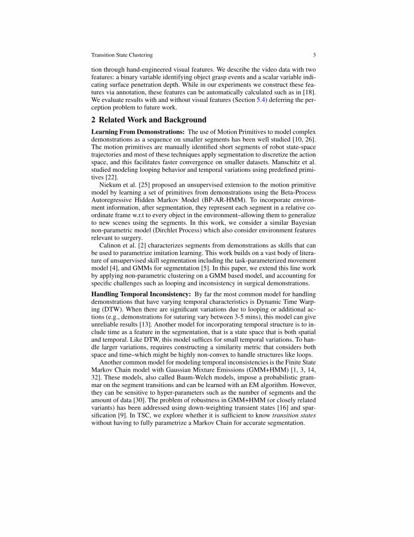
Fig. 2: (1) A finite-state Hidden Markov Chain with Gaussian Mixture Emissions (GMM+HMM) ,and (2) TSC model. TSC uses Dirchilet Process Priors and the concept of transition states to learna robust segmentation.

We design TSC to be robust to some types of variations in demonstrations. In Fig-ure 2, we compare the graphical models of GMM+HMM, and TSC. The TSC modelapplies Dirichlet Process priors to automatically set the number of hidden states(regimes). The goal of the TSC algorithm is to find spatially and temporally similartransition states across demonstrations. On the other hand, the typical GMM+HMMBaum-Welch model learns a k× k transition matrix. We empirically find that theTSC model is robust to noise and temporal variation.Locally Linear Models: Many unsupervised segmentation models either implic-itly or explicitly assume that the dynamics are locally linear. It is important tonote that locally linear dynamics does not imply linear motions, as spiraling mo-tions can be represented as linear systems. In [7], videos are modeled as transitionson a lower-dimensional linear subspace and segments are defined as changes inthese subspaces. Willsky et al [34] proposed BP-AR-HMM, which was applied byNiekum et al. in robotics [25]. This model is explicitly linear by fitting a autoregres-sive model to time-series, where time t +1 is a linear function of times t− k, . . . , t,to windows of data. The linear function switches according to an HMM with statesparametrized by a Beta-Bernoulli model (i.e., Beta Process).

In fact, even the works that apply Gaussian Mixture Models for segmentation [5,19, 15], implicitly fit a locally linear dynamical model. Moldovan et al. [23] provesthat a Mixture of Gaussians model is equivalent to Bayesian Linear Regression; i.e.,when applied to a time window it fits a linear transition between the states.

Local linear models, including the one in this work, can be extended to locallynon-linear models in a straight-forward way through kernelization or increasingtime window. Other non-linear models have been proposed in literature such asLocally Weighted Regression (e.g., see evaluation in [5]). These variants can bethought of as soft-time windows using weighted averages. The choice of linear vs.non-linear is orthogonal to our research contribution of segmentation robust to tem-poral variation.Surgical Task Recognition: Surgical robotics has largely studied the problem ofsupervised segmentation using either segmented examples or a pre-defined dictio-nary of motions (similar to motion primitives). For example, given manually seg-mented videos, Zappella et al. [35] use features from both the videos and kinematic

Transition State Clustering 5

data to classify surgical motions. Simiarly, Quellec et al. [27] use manually seg-mented examples as training for segmentation and recognition of surgical tasksbased on archived cataract surgery videos. The dictionary-based approaches aredone with a domain-specific set of motion primitives for surgery called “surgemes”.A number of works (e.g., [20, 33, 31, 18]), use the surgemes to bootstrap learningsegmentation.

3 Problem SetupThe TSC model is summarized by the hierarchical graphical model in the previ-ous section (Figure 2). Here, we formalize each of the levels of the hierarchy anddescribe the assumptions in this work.

Dynamical System Model: Let D = di be the set of demonstrations where eachdi is a trajectory x(t) of fully observed robot states and each state is a vector in Rd .We model each demonstration as a switched linear dynamical system. There is afinite set of d× d matrices A1, ...,Ak, and an i.i.d zero-mean additive GaussianMarkovian noise process W (t) which accounts for noise in the dynamical model:

x(t +1) = Aix(t)+W (t) : Ai ∈ A1, ...,AkTransitions between regimes are instantaneous where each time t is associated withexactly one dynamical system matrix 1, ...,k

TSC Model (With Visual Sensing) This model can similarly be extended to statesderived from sensing. Suppose at every time t, there is a feature vector z(t). Thenthe augmented state of both the robot spatial state and the features denoted is:

x(t) =(

x(t)z(t)

)In our experiments, we worked the da Vinci surgical robot with with two 7-DOF

arms, each with 2 finger grippers. Consider the following feature representationwhich we used in our experiments:

1. Gripper grasp. 1 if there is an object between the gripper, 0 if not.2. Surface Penetration. In surgical tasks, we often have a tissue phantom. This

feature describes whether the robot (or something the robot is holding like aneedle) has penetrated the surface. We use an estimate of the truncated pene-tration depth to encode this feature. If there is no penetration, the value is 0. Ifthere is penetration, the value of the feature is the robot’s kinematic position inthe direction orthogonal to the tissue phantom.

Transition States and Times: Transition states are defined as the last states beforea dynamical regime transition in each demonstration. Each demonstration di followsa switched linear dynamical system model, therefore there is a time series of regimesA(t) associated with each demonstration.

Therefore, there will be times t at which A(t) 6= A(t + 1). A transition state isthe state x(t) at time t. For a demonstration i, we denote the sequence of transitionsstates as Ui = [u1

i , ...,uJi ]. J is the number of transition states where J Ti where Ti

is the time-length of di.

Transition State Clusters: Across all demonstrations, we are interested in aggre-gating nearby (spatially and temporally) transition states together. A transition state

6 Krishnan, Garg et al.

cluster is defined as a clustering of the set of transition states across all demonstra-tions; partitioning these transition states into m non-overlapping similar groups:

C = C1,C2, ...,CmIn principle, any similarity-based clustering model can be applied, and in the nextsection, we describe using a hierarchical application of DP-GMM by first applyinga GMM to states, and then sub-clustering by applying a GMM to times. Other priorsegmentation works use time as a feature to the GMM, however, this leads to anissue of designing a similarity metric that considers both spatial states and time.Every Ui can be represented as a sequence of integers indicating that transition statesassignment to one of the transition state clusters Ui = [1,2,4,2].

Consistency: We assume, demonstrations are consistent, meaning there exists anon-empty sequence of transition states U ∗ such that the partial order defined bythe elements in the sequence (i.e., s1 happens before s2 and s3) is satisfied by everyUi. For example,

U1 = [1,3,4], U2 = [1,1,2,4], U ∗ = [1,4]A counter example,

U1 = [1,3,4], U2 = [2,5], U ∗ no solutionIntuitively, this condition states that there have to be a consistent ordering of actionsover all demonstrations up to some additional regimes (e.g., spurious actions).

Loops: Loops are common in surgical demonstrations. For example, a surgeon mayattempt to insert a needle 2-3 times. When demonstrations have varying amountsof retrials it is challenging. In this work, we assume that these loops are modeledas repeated transitions between transition state clusters, which is justified in ourexperimental datasets, for example,

U1 = [1,3,4], U2 = [1,3,1,3,1,3,4], U ∗ = [1,3,4]Our algorithm will compact these loops together into a single transition.

Minimal Solution: Given a consistent set of demonstrations, that have additionalregimes and loops, the goal of the algorithm is to find a minimal solution, U ∗ thatis loop free and respects the partial order of transitions in all demonstrations.

Problem 1 (Transition State Clustering Problem). Given a set of demonstrationsD , the Transition State Clustering problem is to find a set of transition state clustersC such that they represent a minimal parametrization of the demonstrations.

4 Transition State ClusteringIn this section, we describe the hierarchical clustering process of TSC. This algo-rithm is a greedy approach to learning the parameters in the graphical model inFigure 2. We decompose the hierarchical model into stages and fit parameters to thegenerative model at each stage. The full algorithm is described in Algorithm 1.

4.1 Background: Bayesian StatisticsOne challenge with mixture models is hyper-parameter selection, such as the num-ber of clusters. Recent results in Bayesian statistics can mitigate some of these prob-lems. The basic recipe is to define a generative model, and then use ExpectationMaximization to fit the parameters of the model to observed data. The generative

Transition State Clustering 7

model that we will use is called a mixture model, which defines a probability distri-bution that is a composite of multiple distributions.

One flexible class of mixture models are Gaussian Mixture Models (GMM),which are described generatively as follows. We first sample some c from a cat-egorical distribution, one that takes on values from (1...K), with probabilities φ ,where φ is a K dimensional simplex:

c∼ cat(K,φ)

Then, given the event c = i, we specify a multivariate Gaussian distribution:xi ∼ N(µi,Σi)

The insight is that a stochastic process called the Dirichlet Process (DP) defines adistribution over discrete distributions, and thus instead we can draw samples ofcat(K,φ) to find the most likely choice of K via EM. The result is the followingmodel:

(K,φ)∼ DP(H,α) c∼ cat(K,φ) X ∼ N(µi,Σi) (1)After fitting the model, every observed sample of x ∼ X will have a probability ofbeing generated from a mixture component P(x | c = i). Every observation x willhave a most likely generating component. It is worth noting that each cluster definesan ellipsoidal region in the feature space of x, because of the Gaussian noise modelN(µi,Σi).

We denote this entire clustering method in the remainder of this work as DP-GMM. We use the same model at multiple levels of the hierarchical clustering andwe will describe the feature space at each level. We use a MATLAB software pack-age to solve this problem using a variational EM algorithm [17].

4.2 Transition States IdentificationThe first step is to identify a set of transition states for each demonstration in D . Todo this, we have to fit a switched dynamic system model to the trajectories. Supposethere was only one regime, then this would be a linear regression problem:

argminA‖AXt −Xt+1‖

where Xt is a matrix where each column vector is x(t), and Xt+1 is a matrix whereeach column vector is the corresponding x(t + 1). Moldovan et al. [23] proves thatfitting a Jointly Gaussian model to n(t) =

(x(t+1)x(t)

)is equivalent to Bayesian Linear

Regression.Therefore, to fit a switched linear dynamical system model, we can fit a Mixture

of Gaussians (GMM) model to n(t) via DP-GMM. Each cluster learned signifiesa different regime, and co-linear states are in the same cluster. To find transitionstates, we move along a trajectory from t = 1, ..., t f , and find states at which n(t) isin a different cluster than n(t +1). These points mark a transition between clusters(i.e., transition regimes).

4.3 Transition State PruningWe consider the problem of outlier transitions, ones that appear only in a fewdemonstrations. Each of these regimes will have constituent vectors where eachn(t) belongs to a demonstration di. Transition states that mark transitions to or fromregimes whose constituent vectors come from fewer than a fraction ρ demonstra-

8 Krishnan, Garg et al.

tions are pruned. ρ should be set based on the expected rarity of outliers. In ourexperiments, we set the parameter ρ to 80% and show the results with and withoutthis step.

4.4 Transition State CompactionOnce we have transition states for each demonstration, and have applied pruning, thenext step is to remove transition states that correspond to looping actions, which areprevalent in surgical demonstrations. We model this behavior as consecutive linearregimes repeating, i.e., transition from i to j and then a repeated i to j. We applythis step after pruning to take advantage of the removal of outlier regimes duringthe looping process. These repeated transitions can be compacted together to makea single transition.

The key question is how to differentiate between repetitions that are part of thedemonstration and ones that correspond to looping actions–the sequence might con-tain repetitions not due to looping. To differentiate this, as a heuristic, we thresholdthe L2 distance between consecutive segments with repeated transitions. If the L2distance is low, we know that the consecutive segments are happening in a simi-lar location as well. In our datasets, this is a good indication of looping behavior.If the L2 distance is larger, then repetition between dynamical regimes might behappening but the location is changing.

For each demonstration, we define a segment s( j)[t] of states between each transi-tion states. The challenge is that s( j)[t] and s( j+1)[t] may have a different number ofobservations and may be at different time scales. To address this challenge, we ap-ply Dynamic Time Warping (DTW). Since segments are locally similar up-to smalltime variations, DTW can find a most-likely time alignment of the two segments.

Let s( j+1)[t∗] be a time aligned (w.r.t to s( j)) version of s( j+1). Then, after align-ment, we define the L2 metric between the two segments:

d( j, j+1) =1T

T

∑t=0

(s( j)[i]− s( j+1)[i∗])2

When d ≤ δ , we compact two consecutive segments. δ is chosen empirically anda larger δ leads to a sparser distribution of transition states, and smaller δ leadsto more transition states. For our needle passing and suturing experiments, we setδ to correspond to the distance between two suture/needle insertion points–thus,differentiating between repetitions at the same point vs. at others.

However, since we are removing points from a time-series this requires us toadjust the time scale. Thus, from every following observation, we shift the timestamp back by the length of the compacted segments.4.5 State-Space ClusteringAfter compaction, there are numerous transition states at different locations in thestate-space. If we model the states at transition states as drawn from a GMM model:

x(t)∼ N(µi,Σi)

Then, we can apply the DP-GMM again to cluster the state vectors at the transitionstates. Each cluster defines an ellipsoidal region of the state-space space.

Transition State Clustering 9

Algorithm 1: The Transition State Clustering Algorithm1: Input: D , ρ pruning parameter, and δ compaction parameter.2: n(t) =

(x(t+1)x(t)

).

3: Cluster the vectors n(t) using DP-GMM assigning each state to its most likely cluster.4: Transition states are times when n(t) is in a different cluster than n(t +1).5: Remove states that transition to and from clusters with less than a fraction of p demonstrations.6: Remove consecutive transition states when the L2 distance between these transitions is less than δ .7: Cluster the remaining transition states in the state space x(t +1) using DP-GMM.8: Within each state-space cluster, sub-cluster the transition states temporally.9: Output: A set M of clusters of transition states and the associated with each cluster a time interval of transition

times.

4.6 Time ClusteringWithout temporal localization, the transitions may be ambiguous. For example, incircle cutting, the robot may pass over a point twice in the same task. The challengeis that we cannot naively use time as another feature, since it is unclear what metricto use to compare distance between

(x(t)t

). However a second level of clustering by

time within each state-space cluster can overcome this issue.Within a state cluster,if we model the times which change points occur as drawn from a GMM:

t ∼ N(µi,σi)

then we can apply DP-GMM to the set of times. We cluster time second because weobserve that the surgical demonstrations are more consistent spatially than tempo-rally. This groups together events that happen at similar times during the demonstra-tions. The result is clusters of states and times. Thus, a transition states mk is definedas tuple of an ellipsoidal region of the state-space and a time interval.

5 Results

5.1 Experiment 1. Synthetic Example of 2-Segment Trajectory

In our first experiment, we segment noisy observations from a two regime lineardynamical system. Figure 3 illustrates examples from this system under the differenttypes of corruption.Evaluation Metric: Since there is a known a ground truth of two segments, wemeasure the precision (average fraction of observations in each segment that arefrom the same regime) and recall (average fraction of observations from each regimesegmented together) in recovering these two segments. We can jointly consider pre-cision and recall with the F1 Score which is the harmonic mean of the two:

f 1 =2 · precision · recallprecision + recall

We compare three techniques against TSC: K-Means (only spatial), GMM+T(using time as a feature in a GMM), GMM+HMM (using an HMM to model thegrammar). For the GMM techniques, we have to select the number of segments, andwe experiment with k = 1,2,3 (i.e., a slightly sub-optimal parameter choice com-pared to k = 2). In this example, for TSC, we set the two user-specified parameters to

10 Krishnan, Garg et al.

−2 −1 0 1 2−2

−1

0

1

2(a) Nominal

X

Y

Regime 1Regime 2

−2 −1 0 1 2−2

−1

0

1

2(b) Noisy Observations

X

Y

Regime 1Regime 2

−2 −1 0 1 2−2

−1

0

1

2(c) Spurious Regime

X

Y

Regime 1Regime 2

−2 −1 0 1 2−2

−1

0

1

2(d) Retrial

X

Y

Regime 1Regime 2

(d) Looping

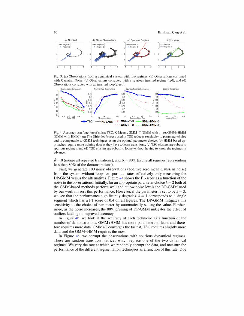
Fig. 3: (a) Observations from a dynamical system with two regimes, (b) Observations corruptedwith Gaussian Noise, (c) Observations corrupted with a spurious inserted regime (red), and (d)Observations corrupted with an inserted loop(green).

0 0.1 0.2 0.3 0.40.4

0.5

0.6

0.7

0.8

0.9

1Segmentation Comparison

F1 S

core

Noise STD0 50 100

0.650.7

0.750.8

0.85

0.90.95

Training Data RequirementsF1

Sco

re

# Demonstrations0 0.1 0.2 0.3

0.650.7

0.750.8

0.85

0.90.95

Spurious Regimes Comparison

F1 S

core

Spurious State Rate0 0.1 0.2 0.3

0.650.7

0.750.8

0.85

0.90.95

Looping Comparison

F1 S

core

Looping Rate

Fig. 4: Accuracy as a function of noise: TSC, K-Means, GMM+T (GMM with time), GMM+HMM(GMM with HMM). (a) The Dirichlet Process used in TSC reduces sensitivity to parameter choiceand is comparable to GMM techniques using the optimal parameter choice, (b) HMM based ap-proaches require more training data as they have to learn transitions, (c) TSC clusters are robust tospurious regimes, and (d) TSC clusters are robust to loops–without having to know the regimes inadvance.

δ = 0 (merge all repeated transitions), and ρ = 80% (prune all regimes representingless than 80% of the demonstrations).

First, we generate 100 noisy observations (additive zero mean Gaussian noise)from the system without loops or spurious states–effectively only measuring theDP-GMM versus the alternatives. Figure 4a shows the F1-score as a function of thenoise in the observations. Initially, for an appropriate parameter choice k = 2 both ofthe GMM-based methods perform well and at low noise levels the DP-GMM usedby our work mirrors this performance. However, if the parameter is set to be k = 3,we see that the performance significantly degrades. k = 1 corresponds to a singlesegment which has a F1 score of 0.4 on all figures. The DP-GMM mitigates thissensitivity to the choice of parameter by automatically setting the value. Further-more, as the noise increases, the 80% pruning of DP-GMM mitigates the effect ofoutliers leading to improved accuracy.

In Figure 4b, we look at the accuracy of each technique as a function of thenumber of demonstrations. GMM+HMM has more parameters to learn and there-fore requires more data. GMM+T converges the fastest, TSC requires slightly moredata, and the GMM+HMM requires the most.

In Figure 4c, we corrupt the observations with spurious dynamical regimes.These are random transition matrices which replace one of the two dynamicalregimes. We vary the rate at which we randomly corrupt the data, and measure theperformance of the different segmentation techniques as a function of this rate. Due

Transition State Clustering 11

to the pruning, TSC gives the most accurate segmentation. The Dirichlet processgroups the random transitions in different clusters and the small clusters are prunedout. On the other hand, the pure GMM techniques are less accurate since they arelooking for exactly two regimes.

In Figure 4d, introduce corruption due to loops and compare the different tech-niques. A loop is a step that returns to the start of the regime randomly, and we varythis random rate. For an accurately chosen parameter k = 2, for the GMM-HMM, itgives the most accurate segmentation. However, when this parameter is set poorlyk = 3, the accuracy is significantly reduced. On the other hand, using time as a GMMfeature (GMM+T) does not work since it does not know how to group loops into thesame regime.

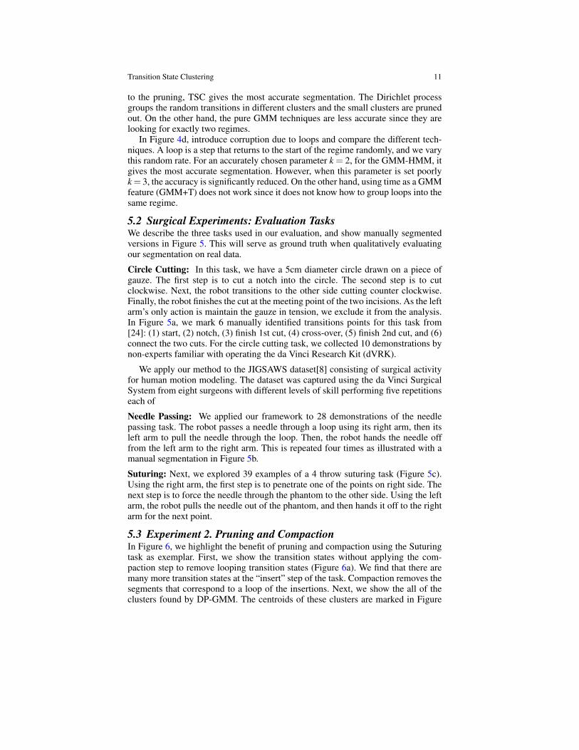
5.2 Surgical Experiments: Evaluation TasksWe describe the three tasks used in our evaluation, and show manually segmentedversions in Figure 5. This will serve as ground truth when qualitatively evaluatingour segmentation on real data.

Circle Cutting: In this task, we have a 5cm diameter circle drawn on a piece ofgauze. The first step is to cut a notch into the circle. The second step is to cutclockwise. Next, the robot transitions to the other side cutting counter clockwise.Finally, the robot finishes the cut at the meeting point of the two incisions. As the leftarm’s only action is maintain the gauze in tension, we exclude it from the analysis.In Figure 5a, we mark 6 manually identified transitions points for this task from[24]: (1) start, (2) notch, (3) finish 1st cut, (4) cross-over, (5) finish 2nd cut, and (6)connect the two cuts. For the circle cutting task, we collected 10 demonstrations bynon-experts familiar with operating the da Vinci Research Kit (dVRK).

We apply our method to the JIGSAWS dataset[8] consisting of surgical activityfor human motion modeling. The dataset was captured using the da Vinci SurgicalSystem from eight surgeons with different levels of skill performing five repetitionseach of

Needle Passing: We applied our framework to 28 demonstrations of the needlepassing task. The robot passes a needle through a loop using its right arm, then itsleft arm to pull the needle through the loop. Then, the robot hands the needle offfrom the left arm to the right arm. This is repeated four times as illustrated with amanual segmentation in Figure 5b.

Suturing: Next, we explored 39 examples of a 4 throw suturing task (Figure 5c).Using the right arm, the first step is to penetrate one of the points on right side. Thenext step is to force the needle through the phantom to the other side. Using the leftarm, the robot pulls the needle out of the phantom, and then hands it off to the rightarm for the next point.

5.3 Experiment 2. Pruning and CompactionIn Figure 6, we highlight the benefit of pruning and compaction using the Suturingtask as exemplar. First, we show the transition states without applying the com-paction step to remove looping transition states (Figure 6a). We find that there aremany more transition states at the “insert” step of the task. Compaction removes thesegments that correspond to a loop of the insertions. Next, we show the all of theclusters found by DP-GMM. The centroids of these clusters are marked in Figure

12 Krishnan, Garg et al.

(a) Circle Cutting

1. Start

2. Notch

3. 1/2 cut

4. Re-enter

6. Finish

5. 1/2 Cut

(b) Needle Passing

1.Start

2.Pass 1

3. Hando!

4. Pass 2

5. Hando!

6. Pass 3

7. Hando!

8. Pass 4

1. Insert

2. Pull

3.Hando! 4. Insert

5. Pull

6.Hando! 7. Insert

10. Insert

8. Pull

9.Hando!

11. Pull

(c) Suturing

Fig. 5: Hand annotations of the three tasks: (a) circle cutting, (b) needle passing, and (c) suturing.Right arm actions are listed in dark blue and left arm actions are listed in yellow.

6b. Many of these clusters are small containing only a few transition states. This iswhy we created the heuristic to prune clusters that do not have transition states fromat least 80% of the demonstrations. In all, 11 clusters are pruned by this rule.

Fig. 6: We first show the transition stateswithout compaction (in black and green),and then show the clusters without pruning(in red). Compaction sparsifies the transi-tion states and pruning significantly reducesthe number of clusters.

0 0.02 0.04 0.06 0.08 0.10

0.02

0.04

0.06

Suturing Change Points: No Compaction

X (m)

Y (

m)

0 0.02 0.04 0.06 0.08 0.10

0.02

0.04

0.06

Suturing Milestones No Pruning

X (m)

Y (

m)

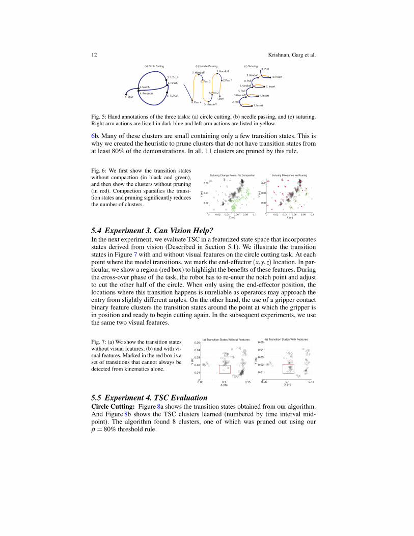
5.4 Experiment 3. Can Vision Help?In the next experiment, we evaluate TSC in a featurized state space that incorporatesstates derived from vision (Described in Section 5.1). We illustrate the transitionstates in Figure 7 with and without visual features on the circle cutting task. At eachpoint where the model transitions, we mark the end-effector (x,y,z) location. In par-ticular, we show a region (red box) to highlight the benefits of these features. Duringthe cross-over phase of the task, the robot has to re-enter the notch point and adjustto cut the other half of the circle. When only using the end-effector position, thelocations where this transition happens is unreliable as operators may approach theentry from slightly different angles. On the other hand, the use of a gripper contactbinary feature clusters the transition states around the point at which the gripper isin position and ready to begin cutting again. In the subsequent experiments, we usethe same two visual features.

Fig. 7: (a) We show the transition stateswithout visual features, (b) and with vi-sual features. Marked in the red box is aset of transitions that cannot always bedetected from kinematics alone.

0.05 0.1 0.150

0.01

0.02

0.03

0.04

0.05

X (m)

Y (

m)

(b) Transition States With Features

0.05 0.1 0.150

0.01

0.02

0.03

0.04

0.05

X (m)

Y (

m)

(a) Transition States Without Features

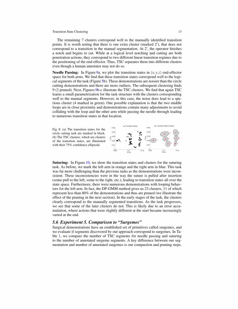
5.5 Experiment 4. TSC EvaluationCircle Cutting: Figure 8a shows the transition states obtained from our algorithm.And Figure 8b shows the TSC clusters learned (numbered by time interval mid-point). The algorithm found 8 clusters, one of which was pruned out using ourρ = 80% threshold rule.

Transition State Clustering 13

The remaining 7 clusters correspond well to the manually identified transitionpoints. It is worth noting that there is one extra cluster (marked 2′), that does notcorrespond to a transition in the manual segmentation. At 2′, the operator finishesa notch and begins to cut. While at a logical level notching and cutting are bothpenetration actions, they correspond to two different linear transition regimes due tothe positioning of the end-effector. Thus, TSC separates them into different clusterseven though a human annotator may not do so.

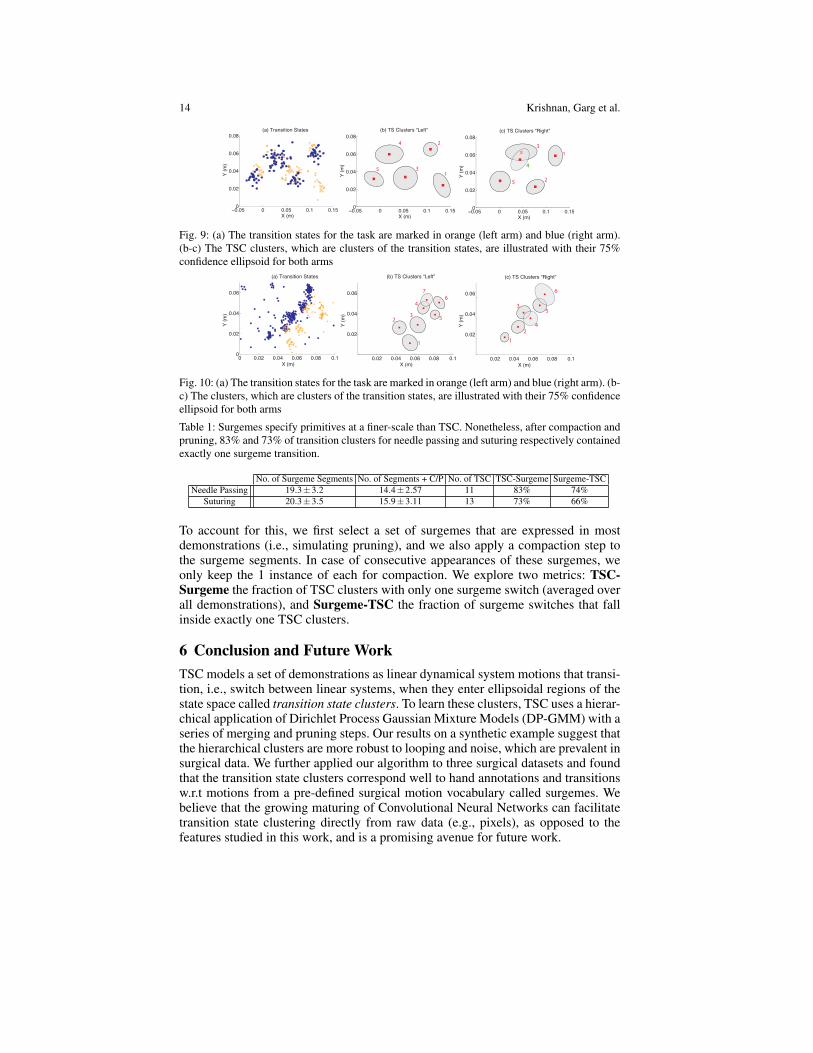
Needle Passing: In Figure 9a, we plot the transition states in (x,y,z) end-effectorspace for both arms. We find that these transition states correspond well to the logi-cal segments of the task (Figure 5b). These demonstrations are noisier than the circlecutting demonstrations and there are more outliers. The subsequent clustering finds9 (2 pruned). Next, Figures 9b-c illustrate the TSC clusters. We find that again TSClearns a small parametrization for the task structure with the clusters correspondingwell to the manual segments. However, in this case, the noise does lead to a spu-rious cluster (4 marked in green). One possible explanation is that the two middleloops are in close proximity and demonstrations contain many adjustments to avoidcolliding with the loop and the other arm while passing the needle through leadingto numerous transition states in that location.

Fig. 8: (a) The transition states for thecircle cutting task are marked in black.(b) The TSC clusters, which are clustersof the transition states, are illustratedwith their 75% confidence ellipsoid.

0.05 0.1 0.150

0.01

0.02

0.03

0.04

0.05

X (m)

Y (

m)

(a) Transition States

0.05 0.1 0.150

0.01

0.02

0.03

0.04

0.05

X (m)

Y (

m)

(b) Transition State Clusters

1

2

2’ 3

4 5

6

Suturing: In Figure 10, we show the transition states and clusters for the suturingtask. As before, we mark the left arm in orange and the right arm in blue. This taskwas far more challenging than the previous tasks as the demonstrations were incon-sistent. These inconsistencies were in the way the suture is pulled after insertion(some pull to the left, some to the right, etc.), leading to transition states all over thestate space. Furthermore, there were numerous demonstrations with looping behav-iors for the left arm. In fact, the DP-GMM method gives us 23 clusters, 11 of whichrepresent less than 80% of the demonstrations and thus are pruned (we illustrate theeffect of the pruning in the next section). In the early stages of the task, the clustersclearly correspond to the manually segmented transitions. As the task progresses,we see that some of the later clusters do not. This is likely due to an error accu-mulation, where actions that were slightly different at the start became increasinglyvaried at the end.

5.6 Experiment 5. Comparison to “Surgemes”Surgical demonstrations have an established set of primitives called surgemes, andwe evaluate if segments discovered by our approach correspond to surgemes. In Ta-ble 1, we compare the number of TSC segments for needle passing and suturingto the number of annotated surgeme segments. A key difference between our seg-mentation and number of annotated surgemes is our compaction and pruning steps.

14 Krishnan, Garg et al.

−0.05 0 0.05 0.1 0.150

0.02

0.04

0.06

0.08(a) Transition States

X (m)

Y (

m)

−0.05 0 0.05 0.1 0.150

0.02

0.04

0.06

0.08

X (m)

Y (

m)

(b) TS Clusters “Left”

−0.05 0 0.05 0.1 0.150

0.02

0.04

0.06

0.08

X (m)

Y (

m)

(c) TS Clusters “Right”

1

2

3

4

5

1

2

4

3

5

Fig. 9: (a) The transition states for the task are marked in orange (left arm) and blue (right arm).(b-c) The TSC clusters, which are clusters of the transition states, are illustrated with their 75%confidence ellipsoid for both arms

0 0.02 0.04 0.06 0.08 0.10

0.02

0.04

0.06

(a) Transition States

X (m)

Y (

m)

0.02 0.04 0.06 0.08 0.1

0.02

0.04

0.06

X (m)

Y (

m)

(b) TS Clusters “Left”

0.02 0.04 0.06 0.08 0.1

0.02

0.04

0.06

X (m)

Y (

m)

(c) TS Clusters “Right”

1

23

4

5

7

6

1

2

3

4

5

6

Fig. 10: (a) The transition states for the task are marked in orange (left arm) and blue (right arm). (b-c) The clusters, which are clusters of the transition states, are illustrated with their 75% confidenceellipsoid for both arms

Table 1: Surgemes specify primitives at a finer-scale than TSC. Nonetheless, after compaction andpruning, 83% and 73% of transition clusters for needle passing and suturing respectively containedexactly one surgeme transition.

No. of Surgeme Segments No. of Segments + C/P No. of TSC TSC-Surgeme Surgeme-TSCNeedle Passing 19.3±3.2 14.4±2.57 11 83% 74%

Suturing 20.3±3.5 15.9±3.11 13 73% 66%

To account for this, we first select a set of surgemes that are expressed in mostdemonstrations (i.e., simulating pruning), and we also apply a compaction step tothe surgeme segments. In case of consecutive appearances of these surgemes, weonly keep the 1 instance of each for compaction. We explore two metrics: TSC-Surgeme the fraction of TSC clusters with only one surgeme switch (averaged overall demonstrations), and Surgeme-TSC the fraction of surgeme switches that fallinside exactly one TSC clusters.

6 Conclusion and Future WorkTSC models a set of demonstrations as linear dynamical system motions that transi-tion, i.e., switch between linear systems, when they enter ellipsoidal regions of thestate space called transition state clusters. To learn these clusters, TSC uses a hierar-chical application of Dirichlet Process Gaussian Mixture Models (DP-GMM) with aseries of merging and pruning steps. Our results on a synthetic example suggest thatthe hierarchical clusters are more robust to looping and noise, which are prevalent insurgical data. We further applied our algorithm to three surgical datasets and foundthat the transition state clusters correspond well to hand annotations and transitionsw.r.t motions from a pre-defined surgical motion vocabulary called surgemes. Webelieve that the growing maturing of Convolutional Neural Networks can facilitatetransition state clustering directly from raw data (e.g., pixels), as opposed to thefeatures studied in this work, and is a promising avenue for future work.

Transition State Clustering 15

Acknowledgments: This research was supported in part by a seed grant from the UC Berke-ley Center for Information Technology in the Interest of Society (CITRIS), by the U.S. NationalScience Foundation under Award IIS-1227536: Multilateral Manipulation by Human-Robot Col-laborative Systems. This work has been supported in part by funding from Google and and Cisco.We also thank Florian Pokorny, Jeff Mahler, and Michael Laskey.

References

[1] Asfour, T., Gyarfas, F., Azad, P., Dillmann, R.: Imitation learning of dual-arm manipulationtasks in humanoid robots. In: Humanoid Robots, 2006 6th IEEE-RAS International Confer-ence on, pp. 40–47 (2006)

[2] Calinon, S.: Skills learning in robots by interaction with users and environment. In: Ubiqui-tous Robots and Ambient Intelligence (URAI), 2014 11th International Conference on, pp.161–162. IEEE (2014)

[3] Calinon, S., Billard, A.: Stochastic gesture production and recognition model for a humanoidrobot. In: Intelligent Robots and Systems, 2004. (IROS 2004). Proceedings. 2004 IEEE/RSJInternational Conference on, vol. 3, pp. 2769–2774 vol.3 (2004)

[4] Calinon, S., Bruno, D., Caldwell, D.G.: A task-parameterized probabilistic model with min-imal intervention control. In: Robotics and Automation (ICRA), 2014 IEEE InternationalConference on, pp. 3339–3344 (2014)

[5] Calinon, S., D’halluin, F., Sauser, E.L., Caldwell, D.G., Billard, A.G.: Learning and repro-duction of gestures by imitation. Robotics & Automation Magazine, IEEE 17(2), 44–54(2010)

[6] Calinon, S., Halluin, F.D., Caldwell, D.G., Billard, A.G.: Handling of multiple constraintsand motion alternatives in a robot programming by demonstration framework. In: HumanoidRobots, 2009. Humanoids 2009. 9th IEEE-RAS International Conference on, pp. 582–588.IEEE (2009)

[7] Elhamifar, E., Vidal, R.: Sparse subspace clustering. In: Computer Vision and Pattern Recog-nition, 2009. CVPR 2009. IEEE Conference on, pp. 2790–2797. IEEE (2009)

[8] Gao, Y., Vedula, S., Reiley, C., Ahmidi, N., Varadarajan, B., Lin, H., Tao, L., Zappella, L.,Bejar, B., Yuh, D., Chen, C., Vidal, R., Khudanpur, S., Hager, G.: The jhu-isi gesture and skillassessment dataset (jigsaws): A surgical activity working set for human motion modeling. In:Medical Image Computing and Computer-Assisted Intervention (MICCAI) (2014)

[9] Grollman, D.H., Jenkins, O.C.: Incremental learning of subtasks from unsegmented demon-stration. In: Intelligent Robots and Systems (IROS), 2010 IEEE/RSJ International Confer-ence on, pp. 261–266. IEEE (2010)

[10] Ijspeert, A., Nakanishi, J., Schaal, S.: Learning attractor landscapes for learning motor prim-itives. In: Neural Information Processing Systems (NIPS), pp. 1523–1530 (2002)

[11] Intuitive Surgical: Annual report 2014. URL http://investor.intuitivesurgical.com/phoenix.zhtml?c=122359&p=irol-IRHome

[12] Kehoe, B., Kahn, G., Mahler, J., Kim, J., Lee, A., Lee, A., Nakagawa, K., Patil, S., Boyd,W., Abbeel, P., Goldberg, K.: Autonomous multilateral debridement with the raven surgicalrobot. In: Int. Conf. on Robotics and Automation (ICRA) (2014)

[13] Keogh, E.J., Pazzani, M.J.: Derivative dynamic time warping. SIAM[14] Kruger, V., Herzog, D., Baby, S., Ude, A., Kragic, D.: Learning actions from observations.

Robotics & Automation Magazine, IEEE 17(2), 30–43 (2010)[15] Kruger, V., Tikhanoff, V., Natale, L., Sandini, G.: Imitation learning of non-linear point-to-

point robot motions using dirichlet processes. In: Robotics and Automation (ICRA), 2012IEEE International Conference on, pp. 2029–2034. IEEE (2012)

[16] Kulic, D., Nakamura, Y.: Scaffolding on-line segmentation of full body human motion pat-terns. In: Intelligent Robots and Systems, 2008. IROS 2008. IEEE/RSJ International Confer-ence on, pp. 2860–2866. IEEE (2008)

16 Krishnan, Garg et al.

[17] Kurihara, K., Welling, M., Vlassis, N.A.: Accelerated variational dirichlet process mixtures.In: Advances in Neural Information Processing Systems, pp. 761–768 (2006)

[18] Lea, C., Hager, G.D., Vidal, R.: An improved model for segmentation and recognition offine-grained activities with application to surgical training tasks. In: WACV (2015)

[19] Lee, S.H., Suh, I.H., Calinon, S., Johansson, R.: Autonomous framework for segmentingrobot trajectories of manipulation task. Autonomous Robots 38(2), 107–141

[20] Lin, H., Shafran, I., Murphy, T., Okamura, A., Yuh, D., Hager, G.: Automatic detectionand segmentation of robot-assisted surgical motions. In: Medical Image Computing andComputer-Assisted Intervention (MICCAI), pp. 802–810. Springer (2005)

[21] Mahler, J., Krishnan, S., Laskey, M., Sen, S., Murali, A., Kehoe, B., Patil, S., Wang, J.,Franklin, M., Abbeel, P., K., G.: Learning accurate kinematic control of cable-driven surgicalrobots using data cleaning and gaussian process regression. In: Int. Conf. on AutomatedSciences and Engineering (CASE), pp. 532–539 (2014)

[22] Manschitz, S., Kober, J., Gienger, M., Peters, J.: Learning movement primitive attractor goalsand sequential skills from kinesthetic demonstrations. Robotics and Autonomous Systems(2015)

[23] Moldovan, T., Levine, S., Jordan, M., Abbeel, P.: Optimism-driven exploration for nonlinearsystems. In: Int. Conf. on Robotics and Automation (ICRA) (2015)

[24] Murali, A., Sen, S., Kehoe, B., Garg, A., McFarland, S., Patil, S., Boyd, W., Lim, S., Abbeel,P., Goldberg, K.: Learning by observation for surgical subtasks: Multilateral cutting of 3dviscoelastic and 2d orthotropic tissue phantoms. In: Int. Conf. on Robotics and Automation(ICRA) (2015)

[25] Niekum, S., Osentoski, S., Konidaris, G., Barto, A.: Learning and generalization of complextasks from unstructured demonstrations. In: Int. Conf. on Intelligent Robots and Systems(IROS), pp. 5239–5246. IEEE (2012)

[26] Pastor, P., Hoffmann, H., Asfour, T., Schaal, S.: Learning and generalization of motor skillsby learning from demonstration. In: Int. Conf. on Robotics and Automation (ICRA), pp.763–768. IEEE (2009)

[27] Quellec, G., Lamard, M., Cochener, B., Cazuguel, G.: Real-time segmentation and recog-nition of surgical tasks in cataract surgery videos. Medical Imaging, IEEE Transactions on33(12), 2352–2360 (2014)

[28] Reiley, C.E., Plaku, E., Hager, G.D.: Motion generation of robotic surgical tasks: Learningfrom expert demonstrations. In: Engineering in Medicine and Biology Society (EMBC),2010 Annual International Conference of the IEEE, pp. 967–970. IEEE (2010)

[29] Rosen, J., Brown, J.D., Chang, L., Sinanan, M.N., Hannaford, B.: Generalized approach formodeling minimally invasive surgery as a stochastic process using a discrete markov model.Biomedical Engineering, IEEE Transactions on 53(3), 399–413 (2006)

[30] Tang, H., Hasegawa-Johnson, M., Huang, T.S.: Toward robust learning of the gaussian mix-ture state emission densities for hidden markov models. In: Acoustics Speech and SignalProcessing (ICASSP), 2010 IEEE International Conference on, pp. 5242–5245. IEEE (2010)

[31] Tao, L., Zappella, L., Hager, G.D., Vidal, R.: Surgical gesture segmentation and recognition.In: Medical Image Computing and Computer-Assisted Intervention–MICCAI 2013, pp. 339–346. Springer (2013)

[32] Vakanski, A., Mantegh, I., Irish, A., Janabi-Sharifi, F.: Trajectory learning for robot program-ming by demonstration using hidden markov model and dynamic time warping. Systems,Man, and Cybernetics, Part B: Cybernetics, IEEE Transactions on 42(4), 1039–1052 (2012)

[33] Varadarajan, B., Reiley, C., Lin, H., Khudanpur, S., Hager, G.: Data-derived models for seg-mentation with application to surgical assessment and training. In: Medical Image Comput-ing and Computer-Assisted Intervention (MICCAI), pp. 426–434. Springer (2009)

[34] Willsky, A.S., Sudderth, E.B., Jordan, M.I., Fox, E.B.: Sharing features among dynamicalsystems with beta processes. In: Advances in Neural Information Processing Systems, pp.549–557 (2009)

[35] Zappella, L., Bejar, B., Hager, G., Vidal, R.: Surgical gesture classification from video andkinematic data. Medical image analysis 17(7), 732–745 (2013)