Transit Timing Observations FromKepler: Ii. Confirmation of Two

Multiplanet Systems via a Non-Parametric Correlation Analysis

The Harvard community has made thisarticle openly available. Please share howthis access benefits you. Your story matters

Citation Ford, Eric B., Daniel C. Fabrycky, Jason H. Steffen, Joshua A. Carter,Francois Fressin, Matthew J. Holman, Jack J. Lissauer, et al.2012. Transit Timing Observations From Kepler: Ii. Confirmationof Two Multiplanet Systems via a Non-Parametric CorrelationAnalysis. The Astrophysical Journal 750 (2) (April 23): 113.doi:10.1088/0004-637x/750/2/113.

Published Version doi:10.1088/0004-637X/750/2/113

Citable link http://nrs.harvard.edu/urn-3:HUL.InstRepos:29990192

Terms of Use This article was downloaded from Harvard University’s DASHrepository, and is made available under the terms and conditionsapplicable to Open Access Policy Articles, as set forth at http://nrs.harvard.edu/urn-3:HUL.InstRepos:dash.current.terms-of-use#OAP

arX

iv:1

201.

5409

v1 [

astr

o-ph

.EP]

25

Jan

2012

ApJ, in pressPreprint typeset using LATEX style emulateapj v. 5/2/11

TRANSIT TIMING OBSERVATIONS FROM KEPLER: II. CONFIRMATION OF TWO MULTIPLANETSYSTEMS VIA A NON-PARAMETRIC CORRELATION ANALYSIS

Eric B. Ford1, Daniel C. Fabrycky2,3, Jason H. Steffen4, Joshua A. Carter5,3, Francois Fressin5, Matthew J.Holman5, Jack J. Lissauer6, Althea V. Moorhead1, Robert C. Morehead1, Darin Ragozzine5, Jason F. Rowe6,7,William F. Welsh8, Christopher Allen9, Natalie M. Batalha10, William J. Borucki6, Stephen T. Bryson6, LarsA. Buchhave11,12, Christopher J. Burke6,7, Douglas A. Caldwell6,7, David Charbonneau5, Bruce D. Clarke6,7,William D. Cochran13, Jean-Michel Desert5, Michael Endl13, Mark E. Everett14, Debra A. Fischer15, ThomasN. Gautier III16, Ron L. Gilliland17, Jon M. Jenkins6,7, Michael R. Haas6, Elliott Horch18, Steve B. Howell6,Khadeejah A. Ibrahim9, Howard Isaacson19, David G. Koch6, David W. Latham5, Jie Li6,7, Philip Lucas20, Phillip

J. MacQueen13 Geoffrey W. Marcy19, Sean McCauliff9, Fergal R. Mullally6,7, Samuel N. Quinn5, ElisaQuintana6,7, Avi Shporer21,22, Martin Still6,23, Peter Tenenbaum6,7, Susan E. Thompson6,7, Guillermo Torres5,

Joseph D. Twicken6,7, Bill Wohler9, and the Kepler Science Team.

ApJ, in press

ABSTRACT

We present a new method for confirming transiting planets based on the combination of transittimingn variations (TTVs) and dynamical stability. Correlated TTVs provide evidence that the pairof bodies are in the same physical system. Orbital stability provides upper limits for the masses ofthe transiting companions that are in the planetary regime. This paper describes a non-parametrictechnique for quantifying the statistical significance of TTVs based on the correlation of two TTVdata sets. We apply this method to an analysis of the transit timing variations of two stars withmultiple transiting planet candidates identified by Kepler. We confirm four transiting planets in twomultiple planet systems based on their TTVs and the constraints imposed by dynamical stability. Anadditional three candidates in these same systems are not confirmed as planets, but are likely to bevalidated as real planets once further observations and analyses are possible. If all were confirmed,these systems would be near 4:6:9 and 2:4:6:9 period commensurabilities. Our results demonstratethat TTVs provide a powerful tool for confirming transiting planets, including low-mass planetsand planets around faint stars for which Doppler follow-up is not practical with existing facilities.Continued Kepler observations will dramatically improve the constraints on the planet masses andorbits and provide sensitivity for detecting additional non-transiting planets. If Kepler observationswere extended to eight years, then a similar analysis could likely confirm systems with multiple closelyspaced, small transiting planets in or near the habitable zone of solar-type stars.Subject headings: planetary systems; stars: individual (KIC 3231341, 11512246; KOI 168, 1102;

Kepler-23, Kepler-24); planets and satellites: detection, dynamical evolution andstability; techniques: miscellaneous

eford@astro.ufl.edu1 Astronomy Department, University of Florida, 211 Bryant

Space Sciences Center, Gainesville, FL 32611, USA2 UCO/Lick Observatory, University of California, Santa

Cruz, CA 95064, USA3 Hubble Fellow4 Fermilab Center for Particle Astrophysics, P.O. Box 500, MS

127, Batavia, IL 605105 Harvard-Smithsonian Center for Astrophysics, 60 Garden

Street, Cambridge, MA 02138, USA6 NASA Ames Research Center, Moffett Field, CA, 94035,

USA7 SETI Institute, Mountain View, CA, 94043, USA8 Astronomy Department, San Diego State University, San

Diego, CA 92182-1221 , USA9 Orbital Sciences Corporation/NASA Ames Research Center,

Moffett Field, CA 94035, USA10 Department of Physics and Astronomy, San Jose State Uni-

versity, San Jose, CA 95192, USA11 Niels Bohr Institute, Copenhagen University, DK-2100

Copenhagen, Denmark12 Centre for Star and Planet Formation, Natural History Mu-

seum of Denmark, University of Copenhagen, DK-1350 Copen-hagen, Denmark

13 McDonald Observatory, The University of Texas, AustinTX 78730, USA

14 National Optical Astronomy Observatory, Tucson, AZ85719, USA

15 Department of Astronomy, Yale University, New Haven, CT06511, USA

16 Jet Propulsion Laboratory/California Institute of Technol-ogy, Pasadena, CA 91109, USA

17 Space Telescope Science Institute, Baltimore, MD 21218,USA

18 Department of Physics, Southern Connecticut State Uni-versity, New Haven, CT 06515, USA

19 Astronomy Department, University of California, Berkeley,Berkeley, CA 94720

20 Centre for Astrophysics Research, University of Hertford-shire, College Lane, Hatfield, AL10 9AB, England

21 Las Cumbres Observatory Global Telescope, Goleta, CA93117, USA

22 Department of Physics, Broida Hall, University of Califor-nia, Santa Barbara, CA 93106, USA

23 Bay Area Environmental Research Institute/NASA AmesResearch Center, Moffett Field, CA 94035, USA

2 Ford et al.

1. INTRODUCTION

NASA’s Kepler spacecraft was launched on March 6,2009, with the goal of characterizing the occurrence ofsmall exoplanets around solar-type stars. The nom-inal Kepler mission was designed to search for smallplanets transiting their host stars by observing targetsspread over 100 square degrees for three and a halfyears (Borucki et al. 2010; Koch et al. 2010). Af-ter an initial period (“quarter” 0; Q0) of collectingengineering data that included observations of a sub-set of the planet search stars, Kepler began collectingscience data for over 150,000 stars on May 13, 2009.On February 1, 2011, the Kepler team released lightcurves observed during the first ∼ 4.5 months of obser-vations (Q0, Q1 and Q2; May 2, 2009-September 16,2009) for all planet search targets via the Multi-MissionArchive at the Space Telescope Science Institute (MAST;http://archive.stsci.edu/kepler/). In this paper,we analyze observations of 2 stars taken through the endof Q6 (September 22, 2010) which will be made publiclyavailable from MAST at the time of publication.Borucki et al. (2011; hereafter B11) reported the re-

sults of an initial search for transiting planets based onan early and incomplete version of the Kepler pipeline.B11 identified 1235 Kepler Objects of Interest (KOIs)that were active planet candidates as of 1 February 2011and had transit-like events observed in Q0-2. For eachof these, B11 Table 2 lists the putative orbital period,transit epoch, transit duration, planet size, and otherproperties. B11 Table 1 lists properties of the host star,largely from pre-launch, ground-based photometry ob-tained in order to construct the Kepler Input Catalog(KIC; Brown et al. 2011). Additional candidates willlikely be identified due to improvements in the Keplerpipeline and the availability of additional data.Many KOIs were quickly recognized as likely astro-

physical false positives (e.g., blends with backgroundeclipsing binaries; EBs) and were reported in B11 Ta-ble 4. For the remaining planet candidates, the Keplerteam reported a “vetting flag” in B11 to indicate whichKOIs are the strongest and weakest planet candidates.B11 estimates the reliability to be: ≥98% for confirmedplanets (vetting flag=1), ∼ 80% for strong candidates(vetting flag=2), and ∼ 60% for less strong candidates(vetting flag=3) or candidates that have yet to be vetted(vetting flag=4). Independent calculations suggest thatthe reliability could be even greater (Morton & Johnson2011).Further follow-up observations and analysis are re-

quired to determine the completeness and false alarmrates as a function of planet and host star properties.Nevertheless, several papers have begun to analyze theproperties of the Kepler planet candidate sample. BothB11 and Howard et al. (2011) assumed that most Keplerplanet candidates are real and analyzed the frequency ofplanets as a function of planet size, orbital period andhost star type. Youdin (2011) performed a complemen-tary analysis of the joint planet size-orbital period distri-bution. Moorhead et al. (2011) analyzed the transit du-ration distribution of Kepler planet candidates and theimplications for their eccentricity distribution. Of partic-ular interest are 115 stars, each with multiple transitingplanet candidates (MTPCs). Latham et al. (2011) com-

pared the planet size and period distributions of theseplanet candidates with those orbiting stars with only onetransiting planet candidate. Lissauer et al. (2011b) ana-lyzed the architectures of such planetary systems. Fordet al. (2011) searched for evidence of transit timing varia-tions (TTVs) based on the transit times measured duringQ0-2. They found 65 TTV candidates and identified adozen MTPC systems which are likely to be confirmed(or rejected)by TTVs measured over the full Kepler mis-sion lifetime. Both Latham et al. (2011) and Lissaueret al. (2011b) point out that the number of false pos-itives in MTPC systems is expected to be much lowerthan the number of false positives for single transitingplanet candidates. Combined with the already low rateof false positives for Kepler planet candidates (B11; Mor-ton & Johnson 2011), we expect very few false positivesamong candidates in MTPC systems. Still, it is impor-tant to test and confirm individual systems, in order toestablish the frequency of planetary systems with smallplanets and identify any unexpected sources of false pos-itives.Already, seven Kepler planets have been confirmed by

TTVs (Kepler-9b&c, Holman et al. 2010; Kepler-11b-f,Lissauer et al. 2011a) and three additionalKepler planetsin MTPC systems have been validated (Kepler-9d, Torreset al. 2011; Kepler-10c, Fressin et al. 2011; Kepler-11g,Lissauer et al. 2011). Previously, discovery papers pre-sented a detailed analysis of all available data for eachconfirmed Kepler planet, often including a wide array offollow-up observations. Given Kepler’s astounding haulof planet candidates, such detailed analyses will not bepractical for all planets.In this paper, we present a new method to confirm

planets based on combining observations of TTVs withthe constraint of dynamical stability. We perform TTVanalyses of 2 MTPC systems that provide strong evi-dence that at least two of the planet candidates aroundeach star are bound to the same host star (as opposed toa blend of two stars each with one planet or two eclipsingbinaries diluted by the target star). Next, we test for dy-namical stability of the nominal multiple planet systemmodel and consider the effect of varying the mass of theplanet candidates. We place upper limits on the massesof planets which show significant TTVs. Finally, we per-form a basic analysis of Kepler observations through Q6and the available follow-up observations to check for anywarning signs of possible false positives. Given the ev-idence for TTVs and the mass limits from dynamicalstability, we confirm 4 planets in 2 MTPC systems.This paper is organized as follows. First, we provide

an overview of Kepler observations for the KOIs consid-ered in §2. Second, we describe a new method for cal-culating the significance of TTVs in MTPC systems in§3.1-3.5. Readers primarily interested in the propertiesof the planetary systems do not necessarily need to readthe details of the statistical methods presented in §3.2-3.4. We describe our use of n-body simulations to obtainupper limits on planet masses in §3.6. In §4, we describethe results of our statistical and dynamical analyses. Wepresent available follow-up observations and additionalanalysis of Kepler data in §5 and discuss each system in-dividually in §6. Finally, we discuss the implications ofour results and prospects of the method for the future in§7.

Confirmation of Two Multiple Planet Systems 3

2. Kepler PHOTOMETRY & TRANSIT TIMES

We measured transit times based on the “corrected”(or PDC) long cadence (LC), optimal aperture photom-etry performed by the Kepler Science Operations Center(SOC) pipeline version 6.2 (Jenkins et al. 2010). The de-tails of the properties of PDC data and how we deal withthe most common complications are described in Ford etal. (2011). For each system, we begin using the sameprocedure to measure transit times in bulk. In short, foreach planet candidate we fold light curves at an initialestimate of the orbital period. For each planet candidate,we fit a transit model to the folded light curve, excludingobservations during the transits of other planet candi-dates. We use the best-fit limb-darkened transit modelas a fixed template when fitting for each transit time.For example, for a three planet system, we first removetransits of KOIs .02 and .03 from the original light curveto measure TTs for KOI .01. Then, we remove transitsof KOIs .01 and .03 from the light curve to measure TTsfor KOI .02. Finally, we remove transits of KOIs .02 and.03 to measure TTs for KOI .01. In some cases, we iter-ate the procedure. This consists of aligning the transitsbased on the initial set of measured TTs to generate anew transit template and remeasuring transit times usingthe new template. The choice of which TTs to measureand which to exclude due to data gaps or anomalies mayalso change upon iteration. See Ford et al. (2011) fordetails about the algorithm for measuring transit times.We estimate the uncertainty in each transit time fromthe covariance matrix.For some planet candidates with shallow transits, each

transit is too shallow for individual transits to be clearlydetected, and a new algorithm by J. Carter was em-ployed. This model attempts to fit only data within fourtransit durations of the suspected mid-transit, and al-lows for a linear baseline, to correct for astrophysical andinstrumental drifts on timescales much longer than thetransit duration. Global transit parameters are solved forto create a template light curve, which is then scannedover each individual transit. In that scanning process, χ2

is densely sampled as a function of the proposed transitmid-time. Because of the low SNR, the shape of χ2 asa function of the midtime can be very skewed and spiky,rather than shaped as a parabola, in the vicinity of thelocal minimum. Therefore, instead of the local curva-ture for an error bar, the algorithm fits a parabola tothe sampled χ2 function, out to ∆χ2 = 7 away fromthe minimum. This parabola thus has a width which ismore stable to noise properties than the local curvatureis, and we adopt its width as the error bar in each point.We employed this method for KOIs 168.03, 1102.01 and1102.02 that are described in detail in §6.We report best-fit linear ephemerides based on transits

observed during Q0-6 in Table 1, along with the numberof transit times observed (nTT), the median timing un-certainty (σTT ) and the median absolute deviation fromthe linear ephemeris (MAD). Transit times measured arereported in Table 2. By definition, positive TTs occurlater than predicted by the linear ephemeris.

3. METHODS

3.1. Statistical Analysis

Visual inspection of TT data sets revealed KOIswith multiple transiting planet candidates including twoplanet candidates which appear to have TTVs that areanticorrelated with each other. In this and two compan-ion papers (Fabrycky et al. 2011; Steffen et al. 2011),we develop complementary methods to establish the sta-tistical significance of apparently correlated TTVs mea-sured in systems of multiple transiting planet candidates.Physically, transit timing variations (relative to a linearephemeris) can only be measured at the times of tran-sit. Since transit times can only be measured at discretetimes and transits of two planets are rarely coincidentwith each other, one can not calculate the standard cor-relation coefficient, since that would require data sam-pled either continuously or at common times. In thissection we develop tools to quantify the extent of thecorrelations between TTV curves and the statistical sig-nificance of the TTVs in MTPC systems.Even if we restrict our attention to systems with only

two planet candidates, there is an astounding varietyof potential TTV signatures (e.g., Veras et al. 2011).For some systems (e.g., in a 1:2 mean motion resonance(MMR) with small libration amplitude), the TTV signa-ture may be relatively simple (e.g., nearly sinusoidal) forthe timespans and timing precision of interest. In thesecases, one might be well served by fitting a parametricmodel to the observations (e.g., polynomial, sinusoid).However, for other systems (e.g., slightly offset from res-onance, modest eccentricity, more than two planets), theTTV signature can be quite complex. Often the shapeand amplitude of the TTVs changes from year to year(or even longer timescales; e.g., Fig 2. of Ford & Hol-man 2007). Given the diversity and potential complexityof TTV signatures, it is necessary to consider a broadrange of functional forms and a large number of modelparameters. Normally, this would raise concerns aboutexploring the high-dimensional parameter space and po-tentially over-fitting data.On a simplistic level, one could address this problem

by smoothing the TTV observations to obtain a contin-uous “TTV curve” for each planet candidate and cal-culate the standard correlation coefficient between thetwo smoothed TTV curves. Of course, the results willdepend on the choice of smoothing algorithm. We over-come the challenges of working with a discrete datasetwith potentially complex structure by the application ofGaussian Processes (GPs). While one could think of theGPs as a fancy smoothing algorithm, there are several at-tractive features of GPs that make them well suited forthis application. In particular, GPs are infinite dimen-sional objects, providing them with enormous flexibilityfor modeling the data. At the same time, their mathe-matical properties make it practical to marginalize overthe infinite dimensional parameter space to calculate, notjust the predictions of a GP for the TTV curve, but alsothe full posterior predictive probability distribution forthe TTV curve at any finite number of times (see §3.3).Thus, we are able to naturally account for the uncertain-ties in the model TTV curve in a fully Bayesian manner.Once we obtain a continuous function for the “TTV

curve” via our GP model, we calculate a Pearson corre-lation coefficient between the GP models for each pair ofneighboring planets. To establish the statistical signif-icance of the apparently correlated TTVs, we calculate

4 Ford et al.

the distribution of correlation coefficients calculated sim-ilarly, but applied to synthetic data sets. Each syntheticdata set is a random permutation of the actual data. Ifthe correlation coefficient calculated from the actual datais more extreme than the 99.9th percentile of the correla-tion coefficients calculated from the simulated data, thenwe conclude that TTVs are sufficiently statistically sig-nificant to consider the planet pair confirmed.

3.2. Overview of Gaussian Processes

Readers who are not interested in the details of thedetails of the statistical methods used to establish thesignificance of TTVs in MTPC systems may choose toskip §3.2-3.4. GPs have been extensively studied and ap-plied in the statistics and machine learning communities(Rasmussen & Williams 2006). GPs have also been ap-plied in a variety of astronomical contexts (e.g., Rybickiet al. 1992; Gibson et al. 2011). A GP defines a dis-tribution over functions. “Process” refers to a methodfor generating a time series of data. “Gaussian” refersto the defining property of a GP that the joint distribu-tion of any finite number of measurements (at discretetimes) has a multi-variate Gaussian distribution, evenwhen conditioned on any combination of observations.While this assumption may seem to be restrictive, GPsare extremely versatile. The assumption of Gaussianityis essential for making it practical to perform computa-tions on the infinite dimensional function space. In par-ticular, for a GP that describes functions of time only(f(t)), a particular GP (GP [m(t), k(t, t′)])is specified bya mean value, m(t), and a covariance function, k(t, t′).Once we adopt a form for the covariance function (i.e.,for particular values for hyperparameters; see §3.3), it be-comes practical to perform Bayesian inference and calcu-late the posterior predictive probability distribution forthe values of f(t) at any number of times.For our application, we can intuitively think of TTVs

as measurements of the value of a function (f(t)) thatis related to how much a planet is ahead (or behind)schedule in its orbit. 24 Of course, Kepler can only makemeasurements of this function at times of transit (or oc-cultation) as viewed by Kepler. Using a Bayesian frame-work, we can calculate the posterior probability distri-bution for f(t∗) at hypothetical observation times (t∗i ),conditioned on the actual measurements of f(t) (i.e.,TTVs) and hyperparameters (θ) that specify the formof the covariance function. We perform this procedurefor each planet candidate in a system. Then, we can cal-culate the correlation coefficient of the GPs for a pair oftransiting planet candidates. We focus our attention onneighboring pairs of transiting planet candidates, mean-ing we do not search for significant correlations betweenplanets if there is an additional transiting planet candi-date with an intermediate period. In order to establishthe statistical significance of the correlation coefficient,we perform the same procedure on synthetic data sets,generated by permuting the order of the TTVs (alongwith their measurement uncertainties). We compare thecorrelation coefficient for the actual TTVs to the distri-bution of correlation coefficients for the synthetic data

24 An alternative interpretation would define a continuum ofhypothetical observers distributed along the orbital plane.

sets to determine a false alarm probability for the exis-tence of TTVs.

3.3. Gaussian Process Model

We model the TTVs of each KOI as an indepen-dent Gaussian Process (GP). Following Rasmussen &Williams (2006), the prior probability distribution forthe values at times (t∗) of a GP with zero mean is

f∗ ≡ f(t∗) ∼ N (0,K (t∗, t∗)) , (1)

where K(t∗, t∗) is the correlation matrix. We assumethat each observed transit time, yi, is normally dis-tributed about the true transit time (f(ti)) and that in-dependent measurement errors have a variance of σ2

obs,i.Then the joint distribution for the actual observationsand a set of hypothetical measurements is[

yf∗

]

∼ N(

0,

[

K (t, t) + σobs2 K (t, t∗)

K (t∗, t) K (t∗, t∗)

])

, (2)

where σ2obs is a diagonal matrix with entries of σ2

obs,i.We can calculate the posterior predictive distribution byconditioning the joint prior distribution on the actualobservations, y. The standard results for the mean (f∗)and covariance (cov(f∗)) of the posterior predictive dis-tribution are

f∗=K(t∗, t)[

K(t, t) + σ2obs

]−1y (3)

cov(f∗)=K(t∗, t∗)−K(t∗, t)[

K(t, t) + σ2obs

]−1K(t, t∗).(4)

For our calculations, we adopt a Gaussian covariancematrix

K(ti, tj ;σr, τ) = σ2r exp

(

− (ti − tj)2

2τ2

)

, (5)

where σr and τ are hyperparameters, describing the am-plitude and timescale of correlations among data points.This choice of a kernel function ensures that the Gaus-sian process is a smooth function (i.e., continuously dif-ferentiable) and allows there to be a single characteristictimescale for TTVs. It can be shown that covariancematrices of this form correspond to Bayesian linear re-gression model with an infinite number of Gaussian basisfunctions (Rasmussen & Williams 2006).In modeling the TTVs as a GP, we are making use of

a posterior predictive distribution for all functions thatare consistent with the observations and the covariancematrix specified by a set of hyperparameters θ. The“trick” of GPs is that we can marginalize over all func-tions analytically using matrix algebra. Fortunately, thelog marginal likelihood conditioned on the hyperparam-eters can also be readily calculated via matrix algebra

log p(y|t, θ)=−1

2yT(

Kθ + σ2obs

)−1y (6)

−1

2log∣

∣Kθ + σ2obs

∣

∣− n

2log 2π, (7)

where Kθ is the correlation matrix K evaluated at theobservation times, t, using a set of hyperparametersθ = {log σr, log τ} (Rasmussen & Williams 2006). Weset σ2

r = median(y2i ), which is equivalent to normalizing

Confirmation of Two Multiple Planet Systems 5

the TTV observations by their median absolute devia-tion. We adopt a value of τ that maximizes the marginallikelihood. We expect this to be a good approximationfor data sets of interest, since the likelihood is typicallysharply peaked for datasets with a significant structure inthe TTV curve. Technically, the marginal likelihood canbe bimodal, with one mode having small τ (correspond-ing to functions that model the observations well) anda second mode with large τ (corresponding to functionsthat basically ignore the measure transit times, attribut-ing them to measurement noise). In principle, one couldexplicitly compare the marginal likelihood of each modeor even use the weighted average of the GPs correspond-ing to the two local maxima. In practice, we found thatthis was not a problem for the data sets considered. Af-ter verifying that the results were not sensitive to theinitial guess for τ , we adopted an initial guess for τ equalto the shorter orbital period of the two planets or 90days (for long period planets). We use the tnmin min-imization package provided by Craig Markwardt25 thatis based on the Newton method for nonlinear minimiza-tion. We find that this algorithm is robust for the datasets considered.We also experimented with Matern class of covariance

functions, which can yield GPs that are less smooth thanthe Gaussian covariance function. The Matern class isparameterized by both a scale τ and a new hyperpa-rameter, ν. In the limit that ν → ∞, the Matern classapproaches the Gaussian covariance function. For half-integer values of ν, the Matern covariance functions canbe written as a polynominal times an exponetial. In par-ticular, we tested ν = 5/2,

K(ti, tj ;σr, τ, ν =5

2)=σ2

r

(

1 +

√5∆ t

τ+

5∆ t2

3τ2

)

(8)

× exp

(

−√5∆ t

τ

)

, (9)

where ∆ t = ti − tj (Rasmussen & Williams 2006).While the choice of covariance function significantly af-fects the smoothness of the predictive distribution, thesignificance of the correlation between two TTV data setsdid not appear to be sensitive to the choice of a Gaus-sian or Maten ν = 5/2 covariance function. Based onour experience analyzing real and simulated data sets,we found that choosing a Gaussian covariance functionand the method of estimating τ described above resultedin a highly robust algorithm. This allowed us to auto-mate our analysis, so that we could perform the MonteCarlo simulations necessary to establish the false alarmrates.

3.4. Correlation Coefficient

Using the GP model for two planet candidates’ TTVcurves, we calculate the mean (fp(t

∗)) and variance(σ2

p(t∗)) of the predictive distribution for each planet,

indicated by the index p. For t∗, we adopt the observedtransit times for both planets combined into a single vec-tor. We calculate a weighted correlation coefficient be-tween the two GP models based on these two samples,

25 http://cow.physics.wisc.edu/$\sim$craigm/idl/idl.html

using weights

wi =(

σ2p(ti) + σ2

q (ti))−1

, (10)

where σ2p and σ2

q refer to the variances of the posteriorpredictive distribution of the Gaussian process (i.e., thediagonal elements of cov(f∗) in Eqn. 3). After concate-nating the weight vectors for the observations times ofthe two planets, the weighted average mean and varianceof the predictive distributions are

〈fp〉 =[

∑

i

wifp(ti)

]

/∑

i

wi (11)

and⟨

σ2p

⟩

=

[

∑

i

wiσ2p(ti)

]

/∑

i

wi. (12)

We calculate the covariance between the two GPs evalu-ated at the actual observation time according to

covp,q =

[

∑

i

wi (fp(ti)− 〈fp〉) (fq(ti)− 〈fq〉)]

/∑

i

wi.

(13)Thus, the correlation coefficient between the two GPs isestimated by

C =covp,q

√

(

covp,p +⟨

σ2p

⟩) (

covq,q +⟨

σ2q

⟩)

(14)

3.5. Establishing the Statistical Significance of TTVs

In order to establish the statistical significance of theputative TTVs for a pair of planet candidates, we applythe same methods described in §3.3 & 3.4 to an ensembleof synthetic datasets. Each synthetic data set includes arandom permutation of the TTVs for each of the planetcandidates. The TTV and measurement uncertainty fora given transit remain paired after permutation. Wesubtract the best-fit linear ephemeris for each syntheticdataset before generating a GP model and calculatingthe weighted correlation coefficients (C′

i) for the ith syn-thetic data set. It is important that we subtract the best-fit linear ephemeris before generating the GP model, sothat any long-term trend in the TTVs is absorbed intothe best-fit orbital period. We consider Nperm = 104 per-muted synthetic data sets. We estimate the false alarmprobability (FAPTTV,C) based on the fraction of syn-thetic data sets for which |C′| is greater than |C| forthe actual pair of TTV curves. In cases where no syn-thetic data sets yield a |C′| as large as |C| for the actualobservations, we report the FAPTTV,C ≤ 10−3.In principle, the above process could result in identify-

ing either a positive or a negative correlation coefficient.We expect that an isolated pair of interacting planetswill have a negative correlation coefficient, reflecting thatenergy is exchanged between the orbits. While this isstrictly true for two planet systems, one could conceiveof a system with additional planets (e.g., a non-transitingplanet that is perturbing both of the planets observed totransit) in which a pair of planets would have a positivecorrelation coefficient. Therefore, we conservatively cal-culate the FAP based on the distribution of the absolute

6 Ford et al.

value of the correlation coefficient, rather than only thefraction of synthetic data sets with C more negative thanthat measured for the actual observations.Several arguments about multiplicity suggest that sys-

tems with MTCPs have a significantly lower false alarmrate than the overall sample of Kepler planets (Lissaueret al. 2011b). We conservatively adopt a threshold falsealarm probability for detecting TTVs of 10−3. Usingsuch a threshold, we expect that the probability of claim-ing significant TTVs for a given pair of planets due toGaussian measurement noise is less than 10−3. Since B11reported 115, 45, 8, 1 and 1 systems with two, three, four,five and six candidate transiting planets, there is a totalof 238 pairs of neighboring planets which we could test(as opposed to 323 total pairs, including non-neighboringpairs). Thus, the expected number of statistical falsealarms from the current sample of multiple planet can-didate systems remains less than one, even if we wereto consider every system with an FAP< 10−3 as con-firmed. In practice, we only claim to confirm those pairsfor which the FAP was robust to outliers (and passed aseries of additional tests).Our estimates of the false alarm probability assume

that each transit time measurement is independent anduncorrelated with other measurements. While there iscorrelated noise in the Kepler photometry, this does notdirectly translate into correlations among measured tran-sit times, since the transits are measured at widely sep-arated times. One possible mechanism for generatingapparently anticorrelated TTs is measurement noise dueto nearly contemporaneous transits of multiple planets.Therefore, our analysis excludes transits that are nearlycoincident with the transit of another known planet can-didate. Physically, it is extremely difficult for an alter-native astrophysical process to cause the large transittiming variations observed in these systems. Aside fromthe gravitational perturbations of the other transitingplanet, the most plausible mechanisms would be starspots. However, generating TT variations on timescaleslonger than a year would require an unusually long-livedspot complex. Further, transit timing noise due to starspots would have an essentially random phase, except inrare cases where the planet orbital period were nearlycoincident with a near integer multiple of the stellar ro-tation period (e.g., Desert et al. 2011a). Such a coin-cidence for multiple planets in one system is even moreunlikely. Finally, the observed TTV amplitude is muchgreater than what can be caused by starspots (Holman etal. 2010). As neither of the stars considered in §6 showlarge rotational modulation, any starspot induced tim-ing variations are negligible relative to TT measurementprecision. Thus, starspots are not a viable explanationof the measured TTVs for either of the stars consideredin §6. Indeed, if there were an autocorrelation of the TTresiduals (TT observations relative to the GP model), themost likely cause would be actual timing variations dueto gravitational perturbations that are not accurately de-scribed by our GP model. Since our GP model allowsfor only a single timescale, an orbital configuration thatresults in multiple TTV timescale would naturally leadto an autocorrelation of the TT residuals. We are opti-mistic that continuedKepler observations will allow us todetect TTVs on multiple timescales, providing more pre-

cise constraints on the masses and orbits of the planetsin these systems (see Fabrycky et al. 2011).

3.6. Dynamical Analysis

To investigate the orbital stability of the system, weconstruct a nominal model based on the measured orbitalperiods with circular and coplanar orbits. In the nominalmodel, we adopt planet masses based on the adoptedplanet radii, and an empirical mass-radius relationship

(Mp/M⊕ = (Rp/R⊕)2.06

; Lissauer et al. 2011ab). Weverify that the nominal model is stable for at least 107

years, including all transiting planet candidates in thesystem.Second, we place upper limits on the masses of the

systems with correlated TTVs by assuming that the realsystem is not dynamically unstable on a short timescale.For placing mass limits, we start from the nominal model,but include only the pair of planets with significantTTVs. (Including additional planet candidates wouldtypically make the system even less likely to be stable.)We inflate the mass of each planet candidate by a com-mon scale factor. We use the same scale factor for themass of both planets, since the relative sizes are well de-termined from the transit light curves (with the possibleexception of grazing transits). A misestimated stellar ra-dius would cause both planets’ sizes and hence nominalmasses by a similar factor. As a misestimated stellarradius would not significantly change the planet-planetsize ratio, the nominal mass ratio for our n-body simula-tions is insensitive to uncertainties in the stellar radius.Another possibility is that both planets sizes could besignificantly underestimated if the light from the targetstar were diluted by light from nearby stars. Again, thiscould significantly affect the planet sizes, but not theplanet-planet size ratio or the planet-planet mass ratiofor our nominal model. A final possibility is that bothplanets with correlated TTVs are transiting a star otherthan the target star, which is diluted by the target star.In this case, the planet radii would be larger than esti-mated by B11, but the ratio of planet radii would stillbe accurately estimated (assuming neither is grazing).Importantly, in each of these cases dynamical stabilitywould still provide upper limits for the masses that showthe bodies to be planets, even if the planetary radii weresignificantly larger than estimated.

4. RESULTS & CONFIRMATION OF Kepler PLANETS

4.1. TTV Analysis & Evidence for Multi-body Systems

Basic information about transit parameters, stellarand planetary properties was presented in B11. A fewkey parameters are reproduced or updated in Tables 1& 3. In Table 4 we report the correlation coefficient(C) for several pairs of neighboring transiting planets,along with the false alarm probability (FAPTTV,C) forthe TTVs based on our correlation analysis and MonteCarlo simulations (see §3.5). The table also includes theratio of transit durations normalized by orbital periodto the one third power (ξ), the 5th or 95th percentileof the distribution of ξ expected for a pair of planetsaround the target host star, the ratios of the root meansquare (RMS) and mean absolution deviation (MAD)of the TTs from the best-fit linear ephemeris for thetwo planets. In the final column, κ gives the ratio of

Confirmation of Two Multiple Planet Systems 7

the measured MAD of TTVs for the two planets to theratio of the predicted TTVs for the same two planets,based on our nominal n-body models. A subset of thesesystems (Kepler-23=KOI 168, Kepler-24=KOI 1102)will be discussed individually in §6. For these systems,we show the measured transit times and the GP modelfor a subset of these systems to be discussed in moredetail in Figures 1- 2. To help illustrate how we calculateC0.001 and FAPTTV,C, we show the histogram of C′

values from synthetic data in Fig. 1 (bottom right panel)for Kepler-23 b&c. The methods developed in thispaper find significant and apparently correlated TTVsin several additional pairs of Kepler planet candidatesthat are to be discussed in Cochran et al. (2011), J.-M.Desert et al. (2011), Fabrycky et al. (2011), Lissauer etal. (2011c), D. Ragozzine et al. (2012, in preparation)and Steffen et al. (2011).

4.2. Dynamical Stability Analysis & Planet Mass Limits

The detection of significant and anti-correlated TTVsprovides strong evidence that the bodies responsible forthe transits are in the same physical system. In principle,one might wonder whether the “transits” could actuallybe eclipses of stellar mass bodies. In order to accountfor the TTVs, the bodies still need to be in the samephysical system. Given the similar orbital periods, anystellar companions would interact very strongly, raisingserious doubts about the long-term dynamical stabilityof the system.We report the maximum planet mass for which our

n-body integrations did not result in at least one bodybeing ejected from the system or colliding with the otherbody or the central star (Table 1; Fig. 3). For each ofthe planets presented in §6, the maximum mass is lessthan 13MJup, excluding a triple star system as a pos-sible false positive. The observed TTVs suggest evenlower maximum masses, but a complete TTV analysiswill require a longer time series of observations. Thereare considerable uncertainties in the stellar masses, butthe available observations preclude us from having un-derestimated the stellar mass by more than a factor oftwo or more, which would be necessary for the maxi-mum stable mass to approach 13MJup. Even ∼ 13MJup

is roughly half of the recently proposed criteria for ex-oplanets (∼ 25MJup; Schneider et al. 2011). Therefore,regardless of the choice of definition, the masses are con-strained to be in the planetary regime.The combination of TTVs and dynamical stability pro-

vides strong evidence that the transits are due to planetsorbiting a common star. Thus, we promote these planetcandidates to confirmed planets. KOI 168.03 and 168.01become Kepler-23b and c, respectively. KOI 1102.02 and1102.01 become Kepler-24b and c, respectively. In §4.3,we show that the probability of the planetary system or-biting a host star other than the original target star isvery small for both of the cases considered in detail.KOIs 168.02, 1102.03 and 1102.04 remain strong planet

candidates. Given the low rate of false positives amongthe Kepler multi-planet candidates, it is quite unlikelythat these KOIs are caused by a blend with a back-ground object. The most likely form of a “false positive”would be another planetary system transiting a secondphysically associated and similar mass star in the Kepler

aperture. Thus, we anticipate that further follow-up ob-servations (such as high-resolution images) and analysis(such as BLENDER) could allow the remaining planetcandidates to be validated as planets. Alternatively, con-tinued Kepler TT observations may allow for dynamicalconfirmation of some of these candidates.

4.3. Identification of Host Star

While the correlated TTVs and dynamical stabilityprovide evidence for a planetary system, it is not yetobvious that the system must orbit the original targetstar. Here we consider the three alternate potential sce-narios that could result in similar appearances: 1) bothplanets orbit a background star, 2) both planets orbita significantly cooler star that is physically associatedwith the target star, and 3) both planets orbit one oftwo physically associated stars of similar mass.The probability of the first case (planetary system

around an unassociated star) can be quantified by con-sidering the range of spectral type and magnitude differ-ences (measured relative to the target star) which couldresult in a transit of the hypothetical background starmimicking the observed transit. Since dynamical sta-bility precludes stellar masses and an object’s radius isinsensitive to its mass in the Jupiter to brown dwarf-mass regime, there is a maximum size for the transit-ing body and the background star must be sufficientlybright that it could result in the observed transit depth(after accounting for dilution by the target star). Themaximum difference in magnitude is ∆Kp,max= 5.3 magfor Kepler-23 and ∆ Kp,max= 2.7 mag for Kepler-24.The potential locations for a background star are con-strained by the observational limits on the centroid mo-tion, i.e., the difference in the location of the flux centroidduring transit and out of transit. We adopt maximumangular separation equal to the 3 − σ confusion radius,0.3” for Kepler-23c and 0.9” for Kepler-24c. Using a Be-sancon galactic model with magnitude and position foreach target star, we estimate the frequncy of backgroundblends that could match the observed transit depth to be∼ 5× 10−4 for Kepler-23 and ∼ 2× 10−3 for Kepler-24.We have not included any constraints on the observedtransit duration or shape. As Kepler continues to ob-serve these systems, we expect that TTVs will eventuallyprovide significant constraints on the orbital eccentrici-ties. Incorporating such a constraint would be expectedto rule out small host stars that would require an apoc-entric transit to match the observed duration. Even ifwe were to assume that large planets are as commonas small planets, then these planetary systems are morethan ∼ 104 and ∼ 5× 102 times more likely to orbit thetarget star than an unassociated background star. Thisexcludes the vast majority of background blends, includ-ing those involving the reddest host stars.Next, we consider the possibility that the target star

might have an undetected stellar companion that couldhost the planetary system. We can exclude blends thatwould result in a color ∆(r − K) ≥ 0.1 magnitudelarger than expected based on a simple set of isochrones(Marigo et al. 2008). Combining photometry from KICand 2MASS, this typically rules out companions in the∼ 0.6−0.8M⊙ range. We will consider nearly equal massbinaries later in this section. If the planets were to or-bit a physically associated star other than the target,

8 Ford et al.

0 100 200 300 400 500 600Time (BJD-2454900)

-60-40

-20

0

20

4060

TT

V (

min

)

0 100 200 300 400 500 600Time (BJD-2454900)

-200

-100

0

100

200

TT

V (

min

)

0 100 200 300 400 500 600Time (BJD-2454900)

-200

-100

0

100

200

TT

V (

min

)

-1.0 -0.5 0.0 0.5 1.0Correlation Coefficient

050

100

150

200

250300

Num

ber

of D

ata

Set

s-1.0 -0.5 0.0 0.5 1.0

Correlation Coefficient

050

100

150

200

250300

Num

ber

of D

ata

Set

s

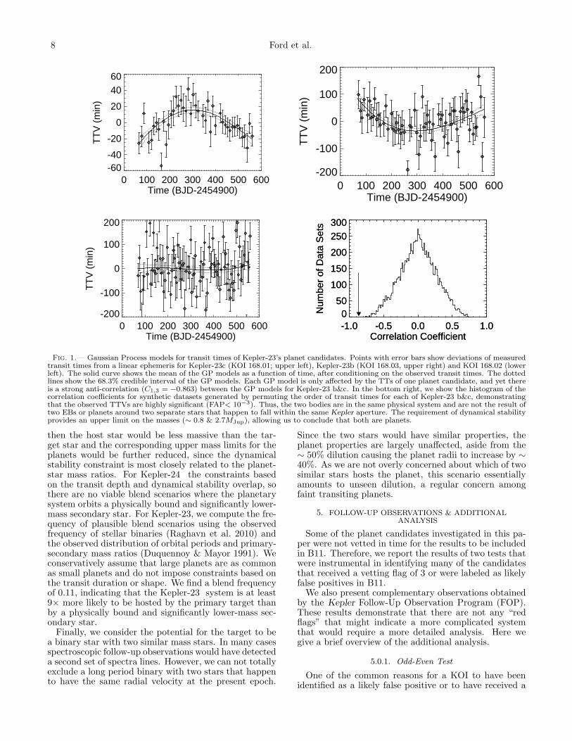
Fig. 1.— Gaussian Process models for transit times of Kepler-23’s planet candidates. Points with error bars show deviations of measuredtransit times from a linear ephemeris for Kepler-23c (KOI 168.01; upper left), Kepler-23b (KOI 168.03, upper right) and KOI 168.02 (lowerleft). The solid curve shows the mean of the GP models as a function of time, after conditioning on the observed transit times. The dottedlines show the 68.3% credible interval of the GP models. Each GP model is only affected by the TTs of one planet candidate, and yet thereis a strong anti-correlation (C1,3 = −0.863) between the GP models for Kepler-23 b&c. In the bottom right, we show the histogram of thecorrelation coefficients for synthetic datasets generated by permuting the order of transit times for each of Kepler-23 b&c, demonstratingthat the observed TTVs are highly significant (FAP< 10−3). Thus, the two bodies are in the same physical system and are not the result oftwo EBs or planets around two separate stars that happen to fall within the same Kepler aperture. The requirement of dynamical stabilityprovides an upper limit on the masses (∼ 0.8 & 2.7MJup), allowing us to conclude that both are planets.

then the host star would be less massive than the tar-get star and the corresponding upper mass limits for theplanets would be further reduced, since the dynamicalstability constraint is most closely related to the planet-star mass ratios. For Kepler-24 the constraints basedon the transit depth and dynamical stability overlap, sothere are no viable blend scenarios where the planetarysystem orbits a physically bound and significantly lower-mass secondary star. For Kepler-23, we compute the fre-quency of plausible blend scenarios using the observedfrequency of stellar binaries (Raghavn et al. 2010) andthe observed distribution of orbital periods and primary-secondary mass ratios (Duquennoy & Mayor 1991). Weconservatively assume that large planets are as commonas small planets and do not impose constraints based onthe transit duration or shape. We find a blend frequencyof 0.11, indicating that the Kepler-23 system is at least9× more likely to be hosted by the primary target thanby a physically bound and significantly lower-mass sec-ondary star.Finally, we consider the potential for the target to be

a binary star with two similar mass stars. In many casesspectroscopic follow-up observations would have detecteda second set of spectra lines. However, we can not totallyexclude a long period binary with two stars that happento have the same radial velocity at the present epoch.

Since the two stars would have similar properties, theplanet properties are largely unaffected, aside from the∼ 50% dilution causing the planet radii to increase by ∼40%. As we are not overly concerned about which of twosimilar stars hosts the planet, this scenario essentiallyamounts to unseen dilution, a regular concern amongfaint transiting planets.

5. FOLLOW-UP OBSERVATIONS & ADDITIONALANALYSIS

Some of the planet candidates investigated in this pa-per were not vetted in time for the results to be includedin B11. Therefore, we report the results of two tests thatwere instrumental in identifying many of the candidatesthat received a vetting flag of 3 or were labeled as likelyfalse positives in B11.We also present complementary observations obtained

by the Kepler Follow-Up Observation Program (FOP).These results demonstrate that there are not any “redflags” that might indicate a more complicated systemthat would require a more detailed analysis. Here wegive a brief overview of the additional analysis.

5.0.1. Odd-Even Test

One of the common reasons for a KOI to have beenidentified as a likely false positive or to have received a

Confirmation of Two Multiple Planet Systems 9

0 200 400 600 800Time (BJD-2454900)

-100

-50

0

50

100

150

TT

V (

min

)

0 200 400 600 800Time (BJD-2454900)

-150

-100

-50

0

50

100

TT

V (

min

)

0 200 400 600 800Time (BJD-2454900)

-150

-100

-50

0

50

100

TT

V (

min

)

0 200 400 600 800Time (BJD-2454900)

-200

-100

0

100

200

TT

V (

min

)

-1.0 -0.5 0.0 0.5 1.0Correlation Coefficient

0

50

100

150

200

250

Num

ber

of D

ata

Set

s

-1.0 -0.5 0.0 0.5 1.0Correlation Coefficient

0

50

100

150

200

250

Num

ber

of D

ata

Set

s

Fig. 2.— Gaussian Process models for transit times of Kepler-24’s planet candidates. Points with error bars show deviations of measuredtransit times from a linear ephemeris for Kepler-24c (KOI 1102.01, upper left) and Kepler-24b (KOI 1102.02, upper right). The solid curveshows the mean of the GP models as a function of time, after conditioning on the observed transit times. The dotted lines show the68.3% credible interval of the GP models. Each GP model is only affected by the TTs of one planet candidate, and yet there is a stronganti-correlation (C1,2 = −0.905) between the GP models for Kepler-24 b&c. At the bottom, we show the histogram of the correlationcoefficients for synthetic datasets generated by permuting the order of transit times for each of Kepler-24 b&c, demonstrating that theobserved TTVs are highly significant (FAP< 10−3). Thus, the two bodies are in the same physical system and are not the result of two EBsor planets around two separate stars that happen to fall within the same Kepler aperture. The requirement of dynamical stability providesan upper limit on the masses (∼ 1.6 & 1.6 MJup), allowing us to conclude that both are planets. While there is significant uncertainty inthe stellar mass, both masses would remain in the planetary regime, even if the stellar mass had been underestimated by a factor of two.

vetting flag of 3 in B11 is a measurement of significantdifference in the transit depth of odd and even numbered“transits”. This can occur if the apparent transit is dueto an EB, where the odd and even “transits” differ inwhich star is eclipsing and which is being eclipsed. (Typ-ically, the EB must also be diluted and/or grazing in or-der for the depth to be consistent with a planet.) TheKepler pipeline provides an odd-even depth test statis-tic that can be used to identify KOIs potentially dueto an EB (Steffen et al. 2010). Inspecting the odd-eventest statistic is also advised to check that the inferredorbital period is not half the true orbital period. Sucha misidentification can arise for low signal-to-noise can-didates, such as KOI 730 (see Lissauer et al. 2011; D.Fabrycky et al. 2012, in preparation). We have verifiedthat the odd-even test statistic is less than 3 for each

of the planets with significantly correlated TTVs that isdiscussed in §6, as well as the other planet candidates inthese systems. In the course of our analysis, we notedthat the originally reported period for KOI 168.02 wasan artifact at one third the period of the updated periodfor KOI 168.02.

5.0.2. Centroid Motion

Another of the common reasons for a KOI to receive avetting flag of 3 in B11 was a measurement of significantdifference in the location of the centroid of the targetstar during transit and out-of-transit. Centroid motioncan be due to to a background EB that is blended withthe target star. On the other hand, small but statisti-cally significant centroid motion does not necessarily im-ply that the KOI is not a planet. For example, local scene

10 Ford et al.

Fig. 3.— Timescale until dynamical instability as a function of planet mass. For each system, we perform a series of n-body integrationsincluding the pair of planets for which we detect significant TTVs with our correlation analysis. We vary the masses of the planets, subjectto the nominal planet-planet mass ratio based on the transit depths. We assume initially circular, coplanar orbits and the nominal stellarmasses in Table 3. Points with an upward arrow indicate n-body integrations which did not go unstable for 107 years. In all cases, themaximum masses that do not go unstable within 107 years are clearly in the planetary regime. Thus, all of the transiting planet candidatesfor which we observe correlated TTVs can not due to an eclipsing binary star that is blended with the target star.

Confirmation of Two Multiple Planet Systems 11

crowding can induce an apparent shift in the photomet-ric centroid, as well as introduce biases in pointspreadfunction (PSF)-fitted estimates of the location of thetransiting object via difference images. Removing thesespurious sources of centroid motion requires extensiveanalysis as described in Bryson et al. (2012, in prepa-ration). Here, we limit ourselves to planet candidateswhere the above biases are negligible, so the apparentcentroid motion is within the 3-sigma statistical errordue to pixel-level noise for most of the quarters of dataanalyzed. None of the planet candidates with correlatedTTVs that are discussed in §6 have statistically signifi-cant centroid motion.

5.0.3. Transit Durations

For targets with multiple transiting planet candidates,the ratio of transit durations can be used as a diagnosticto reject blend scenarios (Holman et al. 2010; Batalha etal. 2011; Lissauer et al. 2011; R. Morehead et al. 2012,in preparation). Therefore, we perform a light curve fit-ting based on Q0-6 data primarily to measure transitdurations. We construct folded light curves based onthe measured transit times (see Table 2). Otherwise, wefollow the fitting procedure of Moorhead et al. (2011).Note that the durations reported in Table 1 are basedon when the center of the planet is coincident with thelimb of the star and that this differs from the durationsreported in B11 that were based on the time intervalbetween first and fourth points of contact. The formerdefinition of duration is less sensitive to the uncertaintiesin the planet size, impact parameter and limb darkening(Colon & Ford 2009; Moorhead et al. 2011). Note thatthe planet candidates discussed in this paper have fainthost stars, so there is often a large uncertainty in the im-pact parameters. In most cases where the impact param-eter is not well-constrained, we adopt a central transit,similar to both B11 and Moorhead et al. (2011).We report the normalized transit duration ratio (ξ ≡

(Tdur,in/Tdur,out)(Pout/Pin)1/3) for each pair of neigh-

boring planets in Table 4. We also calculate ξ5 and ξ95,the 5th and 95th percentile of ξ values obtained fromMonte Carlo simulations of an ensemble of systems withtwo planets with the measured orbital periods and a dis-tribution of impact parameters and eccentricities. Sim-ulations are discarded if both planets do not transit orif transits of one planet would not have been detected(due to grazing transits that would result in a reducedsignal-to-noise ratio). In Table 4, we report ξ5/95 whichis simply ξ5 for pairs with ξ < 1 and ξ95 for pairs withξ > 1. Typically, the distribution of ξ is not far fromsymmetric, so ξ0.95 ∼ 1/ξ0.05. For a few pairs where thetwo planets have substantially different radii, the simu-lated distribution of ξ is asymmetric due to the minimumsignal-to-noise criterion. In all cases, the measured ξ isconsistent with a pair of planets transiting a commonhost star.

5.0.4. Spectra of Host Stars

The Kepler FOP has obtained high-resolution spectraof KOI host stars from the 10m Keck I Observatory, the3m Shane Telescope at Lick Observatory, 2.7m Harlan J.Smith Telescope at McDonald Observatory, or the 1.5mTillinghast Reflector at Fred Lawrence Whipple Obser-vatory (FLWO). The choice of observatory and exposure

time were tailored to produce the desired signal to noise.For some faint stars, an initial low-SNR reconnaissancespectra was used for initial vetting, before obtaining asecond higher SNR spectrum that was used for analy-sis. For Kepler-23, stellar parameters are based on spec-tra from McDonald Observatory and the Nordic OpticalTelescope. Spectra were analyzed by computing the cor-relation function between the observed spectrum and alibrary of theoretical spectra using the tools described inL. Buchave et al. (2012, in preparation). This methodprovides measurements of effective temperature (Teff),metallicity ([M/H]) and surface gravity (log(g)), as wellas a means of recognizing binary companions that wouldproduce a second set of spectral lines. In the case ofKepler-24, we adopt the stellar atmospheric parametersfrom the KIC and reported in Borucki et al. (2011), sincea high quality spectrum is not yet available.We report the adopted stellar atmospheric parameters

in Table 3. We also update the stellar mass and radiusbased on Bayesian comparison to Yonsei-Yale isochrones(Yi et al. 2001).

5.0.5. Imaging of Host Stars

The Kepler mission follow-up observing program in-cludes speckle observations obtained at the WIYN 3.5-mtelescope located on Kitt Peak. Speckle observations ofKepler-23 were used to provide high spatial resolutionviews of the target star to look for previously unrecog-nized close companions that might contaminate the Ke-pler light curve. The speckle observations make use ofthe Differential Speckle Survey Instrument (DSSI), a re-cently upgraded speckle camera described in Horch etal. (2010) and Howell et al. (2011). The DSSI providessimultaneous observations in two filters by employing adichroic beam splitter and two identical EMCCDs as theimagers. The details of how we obtain, reduce, and ana-lyze the speckle results and specifics about how they areused eliminate false positives and aid in transit detectionare described in Torres et al. (2010), Horch et al. (2010),and Howell et al. (2011). The latter paper also presentsthe speckle imaging results for the 2010 observing season.Classical imaging systems provide complementary ob-

servations with a wider field of view. In particular, theLick Observatory 1m Nickel Telescope took an I-bandimage of Kepler-23 with a pixel scale of 0.368”/pixel andseeing of ∼1.5”. For Kepler-24, the 2m Faulkes TelescopeNorth (FTN) provides SDSS-r’ band images with a pixelscale of 0.304 ”/pixel in the default 2 x 2 pixel binningmode, and a typical seeing of ∼ 1.2”. For each target astacked image is generated by combining several imagestaken during the night, or on separate nights, when thetarget is at different positions on the sky. This is done inorder to achieve increased sensitivity for faint stars with-out saturating the bright stars, and to average out thediffraction pattern of the spider vanes supporting the sec-ondary mirror (Since FTN has an alt-azimuth mount thediffraction pattern is different at different sky positions,relative to the positions of the stars).

6. PROPERTIES OF CONFIRMED PLANETARY SYSTEMS

Properties of the host stars from the Kepler Input Cat-alog (KIC; Brown et al. 2011) and planet candidates fromKepler light curve analysis are presented in Borucki et al.2011. Table 3 summarizes the key host star parameters,

12 Ford et al. K00168 I Band Lick 1−m

0 50 100 150 200Pixels

0

50

100

150

200P

ixel

s

0.368"/pixel

10"

Fig. 4.— Upper Left: An I-band image of Kepler-23 from the Lick Observatory 1m Nickel Telescope with 1.2’ on a side. Upper right:A speckle image of Kepler-23 with DSSI at WIYN centered on 880nm with 2.8” on a side. Lower left: A J-band image of Kepler-24 fromUKIRT, 1’ on each side (North is up, East is left). Lower right: A r’-band image of Kepler-24 from FTN with the target (red), KIC objects(green, with KIC ID), and other stars detected in the field (purple) circled. Each circle has a 1” radius.

either from the KIC or the Kepler FOP (when available).The key properties of the planets confirmed in this pa-per, as well as additional planet candidates with inter-esting TTVs, are summarized in Table 1. In this section,we discuss two planetary systems that we confirm basedon correlated TTVs and dynamical stability. Other sys-tems with significant and strongly correlated TTVs arethe subject of separate upcoming papers (Cochran et al.2011; J.-M. Desert et al. 2011b, in preparation; D. Fab-rycky et al. 2012; J. Lissauer et al. 2012; D. Ragozzineet al. 2012, in preparation; Steffen et al. 2012).

6.1. KOI 168

Kepler-23 (KOI 168, KID 11512246, Kp=13.4) hoststhree small planet candidates (168.03, 168.01, 168.02)with orbital periods of 7.10, 10.7 and 15.3 days and radiiof ∼ 3.2, 1.9 and 2.2 R⊕, respectively (B11; N. Batalhaet al. 2012, in preparation). In the course of this anal-ysis, we recognized that the originally reported periodfor KOI 168.02 was an artifact with one third the trueperiod. Initial vetting of KOI 168.01 (planet c, 10.7d)resulted in a vetting flag of 2 and an estimated EB prob-ability of ∼ 3.2× 10−5 (B11), indicating that this candi-

Confirmation of Two Multiple Planet Systems 13

date is very unlikely to be due to a background eclipsingbinary. KOI 168.02 and 168.03 (b) were not vetted intime for B11. Based on the analysis described in §5,we find no evidence pointing towards a false positive forany of the three planet candidates. An analysis of pos-sible centroid motion resulted in 3σ radii of confusion ofRc,23c ∼ 0.3” and Rc,23b ∼ 5”. While the radius of con-fusion for Kepler-23b is relatively large, the mean offsetof the centroid during transit is only ∼ 0.1σ, consistentwith measurement uncertainties. Due to the faint starsand relatively low SNR of the transits, the constraintfor Kepler-23b is relatively weak when compared to Ke-pler planet candidates transiting brighter stars. Never-theless, the centroid measurements are still powerful re-sults. Since the typical optimal aperture for photometryof Kepler-23 is 9 pixels in area (i.e., equivalent to a circu-lar aperture with radius of ∼ 6.7”), excluding locationsfor a potential background EB to within 5” eliminates80% of the optimal aperture phase space for blends withbackground objects. The analysis in §4.3 shows that theprobability of a background eclipsing binary causing oneof Kepler-23 b or c is less than∼ 10−4 and the probabilityof the planets being around a lower mass and physicallybound star is less than ∼ 11%.An I-band image was taken with the Lick Observa-

tory 1m Nickel Telescope on July 10, 2010. There wereno companions visible from ∼2-5” away from the targetstar down to 19th magnitude (see Fig. 4). On Jun 11 and12, 2011, the FOP obtained speckle images of Kepler-23in a band centered on 880nm with width 55nm usingDSSI at WIYN. Seven and five integrations, each con-sisting of 1,000 40-ms exposures were coadded. Theseobservations reveal no secondary sources with a 4-σ lim-iting delta magnitude of 2.94 at 0.2”, increasing to 3.5at 1” and 3.57 at 1.8”. As no new nearby stars wereidentified in either set of observations, we adopt ∼ 2.5%contamination of the Kepler aperture used by the Ke-pler pipeline based on prelaunch photometry, the optimalaperture used for photometry and the PSF.The Kepler FOP obtained two medium-resolution

reconisance spectra of Kepler-23 from McDonaldObservatory (HJD=2455153.643746) and FIES(2455054.576815). The spectra result in stellaratmospheric parameters of Teff = 5760 ± 124K,log(g) = 4.0 ± 0.14 and [M/H]=−0.09 ± 0.14 (L.Buchave et al. 2012, in preparation), consistent withthe stellar properties in the KIC. We compare to theYonei-Yale isochrones and derive values for the stellarmass (1.11+0.09

−0.12M⊙) and radius (1.52+0.24−0.30R⊙) that are

slightly smaller than those from the KIC. We estimate aluminosity of ∼ 2.3L⊙ and an age of ∼ 4− 8Gyr.For Kepler-23b, the SNR of each transit is only ∼ 1.7,

resulting in significant timing uncertainties (σTT = 47minutes). All three planet candidates are clearly iden-tified after folding the light curve at the best-fit orbitalperiod (Fig. 5). Ford et al. (2011) noted that Kepler-23cwas a TTV candidate based on an offset in the transitepoch between the best-fit linear ephemerides based onQ0-2 and Q0-5. TTVs for Kepler-23b were not recog-nized based on Q0-2 observations alone.The correlation coefficient between the GP models for

TTs of Kepler-23 b&c is C = −0.86, well beyond thedistribution of correlation coefficients calculated basedon synthetic data sets with scrambled transit times (see

Fig. 1). The false alarm probability for such an extremecorrelation coefficient is < 10−3. The correlation coeffi-cient between the GP models for TTs of Kepler-23c andKOI 168.02 is -0.23 with a FAP∼ 12%. This is well aboveour threshold for claiming a planet detection. We do notyet detect statistically significant TTVs for 168.02, as ex-pected due to the smaller predicted TTV signal for KOI168.02 and the sizable timing uncertainties. In combina-tion with the analysis of Kepler light curves and FOP ob-servations described above, the strongly anti-correlatedTTVs of Kepler-23 b & c provide a dynamical confirma-tion that the two objects orbit the same star.Kepler-23 b&c have short orbital periods and lie close

to a 3:2 resonance: P23b/P23c = 1.511. Therefore, weexpect a relatively short TTV timescale:

PTTV = 1/(3/10.7421d− 2/7.1073d) = 470d. (15)

The observed timescale (∼ 455d) and phase of TTVs forKepler-23 b&c are consistent with expectations based onn-body integrations using nominal planet mass estimatesand circular, coplanar orbits (see Fig. 6). The amplitudeof the observed TTVs is ∼ 5 times larger than the nomi-nal model. Such differences are not unexpected, as evenmodest eccentricities can significantly increase the TTVamplitude (e.g., Veras et al. 2011). The prediction of thenominal model for the ratio of the TTV amplitudes of thetwo confirmed planets is significantly more robust thanthe predictions of individual amplitudes. Indeed, the ob-served MAD TTV from a linear ephemeris is within 5%of that predicted by the nominal model. Our GP mod-els for the TTs of Kepler-23 b&c are non-parametric,so there is nothing in our model that would cause theGPs to match the ratio of TTV amplitudes, the TTVperiod, or the phase of TTV variations. The fact thatour general non-parametric model naturally reproducesthese features provides an even more compelling case forthe confirmation of these planets via TTVs.While the currently available data is insufficient for

robust determinations of the planet masses, we fit twon-body models to the TTV observations. If we assumeinitially circular and coplanar orbits, then the best-fitmasses are ∼ 22 ± 6 and 12 ± 2M⊕. If we assume ec-centric coplanar orbits, then the best-fit masses are ∼ 15and 5M⊕, corresponding to orbital solutions with loweccentricities. Significantly smaller or larger masses arepossible, but these require large eccentricities. Eithermodel represents a significant improvement in the qual-ity of the fit relative to a non-interacting model. Despitethe sizable uncertainties in the estimates for the planetmasses, the requirement of dynamical stability providesfirm upper limits (2.7 & 0.8 MJup) on the planet masses(Fig. 3).

6.2. Kepler-24 (KOI 1102)

Kepler-24 (KOI 1102, KID 3231341, Kp=14.9) hostsfour planet candidates (04, 02, 01 and 03) with orbitalperiods of 4.2, 8.1, 12.3, 19.0 days and radii of 1.7, 2.4,2.8, 1.7 R⊕, respectively (see Fig. 7; B11; N. Batalha etal. 2012 in preparation). KOI 1102.02 (b) and 1102.01 (c)were identified, but not vetted in time for B11. Based onthe analysis described in §5, we find no evidence pointingtowards a false positive for any of KOI 1102.01-1102.04.The centroids during transit for Kepler-24b & c differ

14 Ford et al.

Fig. 5.— Kepler Light curve for Kepler-23. Panel a shows the raw calibrated Kepler photometry (PA) and panel b shows the photometryafter detrending. The transit times of each planet are indicated by dots at the bottom of each panel. The bottom, middle and top rows ofdots (yellow, red, blue) are for Kepler-23 b, c and KOI 168.02. The lower three panels show the superimposed light curve for each transit,after shifting by the measured mid-time, for Kepler-23b, c and KOI 168.02.

Confirmation of Two Multiple Planet Systems 15

Fig. 6.— Comparison of measured transit times (left) and transit times predicted by the nominal model (right) for a system containingonly Kepler-23b (top) and c (bottom). The model assumes circular and coplanar orbits and nominal masses, as described in §3.6 and Table3. The red curves on the left show the best-fit sinusoidal model with a period constrained to be that predicted by measured orbital periods(see Fabrycky et al. 2011 for details). The red error with no point at the far left shows the best-fit amplitude.

16 Ford et al.

from those out-of-transit by ∼1.4 and 2.8σ, consistentwith measurement uncertainties, particularly when con-sidering the actual distribution of the apparent centroidmotion during transit is highly non-Gaussian for otherwell-studied cases (Batalha et al. 2010). The ∼ 3σ radiiof confusion are 1.2” and 0.9”, for Kepler-24 b & c,respectively. Based on a preliminary analysis of datathrough Q8, the centroid offsets for 1102.04 and 1102.03are less than 3σ. Again, the limited centroid motionenables us to exclude the locations for potential back-ground EBs to a small fraction of the optimal aperturephase space for blends with background objects. Theanalysis in §4.3 shows that the probability of a back-ground eclipsing binary causing one of KOI 1102.01 (c)or 1102.02 (b) is less than ∼ 2× 10−3. The only accept-able blend scenario involves a pair of similar mass andphysically bound stars.A UKIRT J-band image (Fig. 4, left) reveals a faint

companion that is not in the KIC ∼ 2.5” to the SE, withbrightness intermediate to the outlying faint stars KIC3231329 (Kp= 19.0) and KIC 3231353 (Kp= 20.0). AnFTN image also reveals the nearby star, ∼ 5 magnitudesfainter than the target in the r’-band (Fig. 4, right). Weestimate that it is∼ 4−5 magnitudes fainter than Kepler-24 in the Kepler band. As most of its light falls in theKepler image and star is not in the KIC, it results in ∼1−3% dilution in addition to the∼ 8% dilution estimatedby the pipeline for a total of 8.6%.The Kepler FOP has not yet obtained a spectrum

of Kepler-24. We estimate the stellar properties basedon multi-band photometry from the Kepler Input Cat-alog: Teff = 5800 ± 200, log(g) = 4.34 ± 0.3 and[M/H]=−0.24± 0.40. We estimate uncertainties basedon a comparison of KIC and spectroscopic parame-ters for other Kepler targets (Brown et al. 2011). Wederive values for the stellar mass (1.03+0.11

−0.14M⊙), ra-

dius (1.07+0.16−0.23R⊙), luminosity ∼ 1.16+0.36

−0.60 L⊙ and age≤ 7.7Gyr by comparing to the Yonei-Yale isochrones.We caution that there are significant uncertainties asso-ciated with the stellar models and derived properties.Kepler-24 is sufficiently faint that transit times for

Kepler-24c and Kepler-24b have sizable uncertainties(σTT = 30, 25 min). Ford et al. (2011) did not find sig-nificant evidence for TTVs in either of the planet can-didates, but noted that Kepler-24b was likely to havesignificant TTVs (∼ 26 min), based on numerical inte-grations of two planet systems with nominal masses andcircular orbits.The correlation coefficient between the GP models for

TTs of Kepler-24b & c is C = −0.905, well beyond thedistribution of correlation coefficients calculated basedon synthetic data sets with scrambled transit times (seeFig. 2). The false alarm probability for such an extremecorrelation coefficient is < 10−3. In combination withthe analysis of Kepler light curves described above, thisprovides a dynamical confirmation that the two objectsorbit the same star.Kepler-24b & c have short orbital periods and lie near a

3:2 resonance: P24c/P24b = 1.514. Therefore, we expecta relatively short TTV timescale:

Pttv = 1/(2/8.1451d− 3/12.3336d) = 421d. (16)

The observed timescale (∼ 400d) and phase of TTVs

for Kepler-24 b & c are consistent with the expectationsbased on n-body integrations using nominal planet massestimates and circular, coplanar orbits (see Fig. 8). OurGP models for the TTs of Kepler-24 b & c are non-parametric, so there is nothing in our model that wouldcause the GPs to match the period and phase of the TTVvariations. The fact that our general non-parametricmodel naturally reproduces these features provides aneven more compelling case for the confirmation of theseplanets via TTVs.The best-fit amplitudes of the observed TTVs are ∼ 7

and 9 times larger than the nominal model for Kepler-24b& c, respectively. Such differences are not unexpected, aseven modest eccentricities can significantly increase theTTV amplitude (e.g., Veras et al. 2011). Like Kepler-23,the prediction of the nominal model for the ratio of theTTV amplitudes of the two confirmed planets is within25% of the observed ratio (1.25). Still, there could besignificant differences between the true masses and thenominal masses, e.g., if there are significant eccentrici-ties and/or perturbations from other planets in the sys-tem. Assuming that KOI 1102.03 is indeed a planet inthe same system, then Kepler-24c would be near a 3:2MMR with both Kepler-24b (inside) and KOI 1102.03(outside), leading to complex dynamical interactions.While the currently available data is insufficient for

robust determinations of the planet masses, we fit twon-body models to the TTV observations. If we assumeinitially circular and coplanar orbits, then the best-fitmasses are ∼ 17 ± 4 and 5 ± 3M⊕. If we assumeeccentric coplanar orbits, then the best-fit masses are∼ 102 ± 21 and 56 ± 16M⊕, corresponding to orbitalsolutions with eccentricities of ∼ 0.2− 0.4. Either modelrepresents a significant improvement in the quality of thefit relative to a non-interacting model. While the best-fiteccentric model represents a significant improvement inthe goodness-of-fit relative to the best-fit circular model,such large eccentricities may complicate long-term stabil-ity, particularly if all four of the planet candidates wereconfirmed. Despite the sizable uncertainties in the esti-mates for the planet masses, the requirement of dynam-ical stability provides a firm upper limit on the planetmasses (1.6 & 1.6MJup; Fig. 3).We do not detect a statistically significant correla-

tion coefficient between TTVs of either KOI 1102.03 or1102.04 and any of the other planet candidates. Thescatter of the TTVs for 1102.04 is consistent with themeasurement uncertainties. One can understand the lackof a TTV detection for KOI 1102.04 analytically, sincethe amplitude of a TTV signal scales with the orbitalperiod, KOI 1102.04 has an orbital period roughly halfthat of Kepler-24b, and the TTV signal for Kepler-24bis near the limit of detectability. Further, the transit ofKOI 1102.04 is shallower than Kepler-24b, so the TTVsare less precise. If KOI 1102.04 is a planet in the samesystem, then the current innermost period ratio wouldbe P24b/P1102.04 = 1.92, ∼ 5% less than 2, whereas itis more common for systems near a 1:2 MMR to have aperiod ratio ∼ 5% greater than 2 (Lissauer et al. 2011b).This could be related to the presence of four planet can-didates with orbital period ratios near a 2:4:6:9 resonantchain. The current period ratios for the outer two pairs(P24c/P24b = 1.514 and P1102.03/P24c = 1.54) are slightlygreater than 1.5, so none of the neighboring pairs are nec-

Confirmation of Two Multiple Planet Systems 17

essarily “in resonance”. Such deviations from an exactperiod commensurability appear to be common amongKepler planet candidates (Lissauer et al. 2011).There may be early hints of excess scatter in the TTVs

of 1102.03, but this is not statistically significant basedon the current data set. If KOI 1102.03 is a planet inthe same system, then Kepler-24c would feel significantperturbations from both Kepler-24b (on the inside) and1102.03 (on the outside). This may help explain why theobserved TTVs for Kepler-24b are significantly greaterthan those predicted by the nominal two-planet modelthat includes only planets b & c. We hope that this paperwill motivate more detailed analysis of the TTVs andorbital dynamics of this fascinating planetary system.

18 Ford et al.

Fig. 7.— Kepler Light curve for Kepler-24. Panel a shows the raw calibrated Kepler photometry (PA) and panel b shows the photometryafter detrending. The transit times of each planet are indicated by dots at the bottom of each panel. From from top to bottom, the rows ofdots (yellow, red, blue, green) are for KOI 1102.04, Kepler-24b, Kepler-24c and KOI 1102.03. The lower four panels show the superimposedlight curve for each transit, after shifting by the measured mid-time for each of the four KOIs.

Confirmation of Two Multiple Planet Systems 19

Fig. 8.— Comparison of measured transit times (left) and transit times predicted by the nominal model (right) for a system containingonly Kepler-24b (top) and Kepler-24c (bottom). Details are described in the caption to Fig. 6.

20 Ford et al.

7. DISCUSSION

In this paper and two companion papers (Fabrycky etal. 2011, Steffen et al. 2011), we have described a newapproach to confirming transiting planets. For systemswith MTPCs, correlated TTVs provide strong evidencethat both transiting objects are in the same system. Dy-namical stability provides an upper limit on the masses ofthe transiting bodies. For closely-spaced pairs, the massupper limit is often in the planetary regime, allowingplanets to be confirmed by the combination of correlatedTTVs and the constraint of dynamical stability.We have described a non-parametric method for quan-

tifying the significance of TTVs among MTPC systems.Our approach uses a GP model to allow for a rigorous,yet computationally tractable, Bayesian analysis of eachplanet candidate’s TTV curve. Provided there is a suf-ficient number of transit observations, our correlation-based analysis is more sensitive and robust than test-ing for TTVs of each planet individually (e.g., Ford etal. 2011). N-body simulations show that TTVs of twointeracting planets are correlated, regardless of the ex-act mechanims responsible for the TTVs (e.g., resonantinteraction, indirect effect on the star, secular preces-sion). Thus, our algorithm is designed to be most sen-sitive for detecting TTVs when applied to systems withcorrelated TTVs. Another advantage of this method isthat it makes minimal assumptions about the potentialTTV signatures. This approach is complementary toother methods of quantifying the significance of TTVsin MTPC systems (Fabrycky et al. 2011; Steffen et al.2011). Since the method of Steffen et al. (2011) assumessinusoidal TTV signals, it is expected to be more sen-sitive to systems with sinusoidal TTVs, but less sensi-tive to systems with more complex TTV signatures. Themethod of Fabrycky et al. (2011) assumes that the TTVscan be approximated as sinusoidal and that the dominantTTV timescale can be predicted based on the period ofa known, transiting planet. Since this method performsa minimal number of statistical tests, it is expected tohave an even greater sensitivity for many systems. Ofcourse, it could overlook systems where the TTV signalis more complex or dominated by the perturbations ofa non-transiting planet. Therefore, it will be useful toapply all three methods for detecting TTVs to the Ke-pler MTPC systems. We anticipate that the algorithmdescribed here may be particularly useful for confirmingclosely-spaced systems or systems with more than twoplanets contributing to the TTV signature.We have applied our method to 10 MTPC systems to

calculate the correlation coefficient between TTV curvesfor neighboring transiting planet candidates. Eight ofthese systems have at least one pair of neighboring plan-ets with correlated TTVs for which the TTVs are signif-icant at better than the 10−3 level (see Table 4). Thisdemonstrates that the planet candidates are in the samephysical system. Given their close proximity, the require-ment of dynamical stability provides limits on the max-imum masses that are firmly in the planetary regime.This combination of correlated TTVs plus dynamical sta-bility provides dynamical confirmation of planet candi-dates originally identified photometrically by the Keplermission.While correlated TTVs clearly demonstrate that the

planets orbit the same star, it is not guaranteed thatthe host star is the target. Based on follow-up imag-ing and limits on the extent of centroid motion duringtransit, blends with background objects are extremelyunlikely. However, it is possible that both planets or-bit a physically associated star that is too close to theprimary target star to be identified by imaging, but farenough away that it does not destabilize the system. Ifthe host star were significantly less massive and less lumi-nous than the primary target star, then the planets wouldhave smaller masses, but be much larger in size, sincethe transit depths would be highly diluted by the pri-mary target star. While this is not a viable scenario forKepler-24, we estimate there is a ≤ 11% chance that theKepler-23 planetary system orbits a significantly lowermass star that is physically bound to the primary targetstar. Alternatively, if the secondary is nearly the samemass and luminosity as the primary target star, then thestellar properties would be quite similar, but the planetsizes could be larger by a factor of ∼

√2, due to the ex-

tra dilution. The probability for such scenarios is small,but not completely negligible (e.g., a few percent for KOI738; Fabrycky et al. 2011). In any case, the correlatedTTVs and the mass limits from dynamical stability stilldemonstrate that there are at least two planets in thesame system, despite the uncertainty in stellar parame-ters.This paper presents 2 planetary systems (Kepler-23 &

Kepler-24) containing 4 confirmed planets. Both pairs(Kepler-23b(03) & c(01); Kepler-24b(02) & c(01) ) ofconfirmed planets are near the 3:2 MMR. Each of thesesystems contains additional transiting planet candidateswhich have yet to be confirmed. If confirmed, these sys-tems would contain closely-spaced near-resonant chainsof transiting planets (4:6:9 for Kepler-23 and 2:4:6:9for Kepler-24). Resonant chains can form via migrationthrough a protoplanetary disk (e.g., Cresswell & Nelson2006, 2008), but forming chains of near-resonant plan-ets may be more challenging. More detailed modeling ofthe TTV curve will become a powerful tool for learningabout these systems and planet formation and migration(Ragozzine & Holman 2010), particularly once multiplecycles of TTVs have been measured by Kepler.At the moment, the time span of observations is not yet

sufficient to enable precise mass measurements of planetsin these systems due to degeneracies with the other or-bital properties. Nevertheless, we can already recognizeone of the timescales of the observed TTVs for each sys-tem. For each of the confirmed planets, this timescale isconsistent with the predictions of a nominal model, usingcoplanar, circular orbits and planet masses crudely esti-mated from their radii and the host star properties. Ad-ditionally, the phases of the TTV curves for Kepler-23b& c and Kepler-24b&c are consistent with the predictionsof the nominal model.The observed TTV amplitudes (measured in terms of

the mean absolute deviation from a linear ephemeris)are larger (factors of ∼ 5.3 for Kepler-23, and ∼5-46 forKepler-24) than the predictions of our nominal models.Again, this is not unexpected due to the extreme sensitiv-ity of TTVs to masses and eccentricities. The ratio of theTTV amplitudes for each pair of planets with correlatedTTVs is a more robust prediction, as several sources of

Confirmation of Two Multiple Planet Systems 21

uncertainty affect both planet masses similarly (i.e., stel-lar mass, amount of dilution of Kepler light curve). In-deed, we find excellent agreement (∼ 1 − 2%) betweenthe ratio of observed TTV amplitudes and with the cor-responding prediction of the nominal model for Kepler-23b & c. For Kepler-24, this ratio is ∼ 0.1, perhaps dueto significant eccentricities or perturbations from KOI1102.03.We caution that the uncertainty in the masses and sizes

of the host stars directly translates into uncertainties inthe planet masses and sizes. As the time span of Ke-pler TTV observations increases, more detailed dynam-ical analyses will become possible. Additional follow-upobservations and analysis will become increasingly im-portant to aid in the interpretation of the detailed dy-namical information contained in the TTV curves forthese systems.Alternative techniques for studying TTVs of MTPC

systems also confirm the TTVs of Kepler-23 and Kepler-24 with a false alarm probability of < 10−3 (Fabrycky etal. 2011; Steffen et al. 2011). The GP method here is no-table for its minimal set of assumptions, making it mostsensitive for large data sets, even if the observed TTV sig-nature is complex and differs from that expected. Thus,the GP method could prove particularly valuable for an-alyzing TTVs of planets that are significantly perturbedby a non-transiting planet and/or multiple planets.The planets confirmed here and in companion papers

(Fabrycky et al. 2011; Steffen et al. 2011) are not meantto represent an exhaustive search of the Kepler planetcandidates presented in B11. With continued Keplerobservations, this and other complementary techniques(e.g., Fabrycky et al. 2011; Lissauer et al. 2011bc; Stef-fen et al. 2011) are poised to confirm many more MTPCsystems. In particular, there are several other MTPCsystems near the 3:2 MMR, 2:1 MMR or other periodcommensurabilities that are predicted to have observableTTV signatures (Ford et al. 2011; Lissauer et al. 2011).For many of these KOIs additional analysis and/or ob-servations will be required before their planets can beconfirmed.Due to larger stellar activity than originally antici-

pated (Gilliland et al. 2011), for Kepler to measure the

frequency of Earth-size planets in the habitable zone ofsolar-type stars an extended mission is required. For-tunately, the spacecraft carries consumables that couldsupport an extended mission which would improve sen-sitivity for detecting small planets. An extended mis-sion would also dramatically improve the constraints onplanet masses and orbits based on TTVs for systems suchas those presented here. Indeed, of the four planets con-firmed here, only one was recognized as a TTV candidatein Ford et al. (2011). As the time span of observations in-creases, we anticipate that TTVs will become detectablefor even more systems. An extended mission could alsosubstantially increase the number of transits observed forplanets at longer orbital periods. This would be particu-larly valuable for confirming small planets in or near thehabitable zone.

Funding for this mission is provided by NASA’s ScienceMission Directorate. We thank the entire Kepler teamfor the many years of work that is proving so successful.E.B.F acknowledges support by the National Aeronauticsand Space Administration under grant NNX08AR04G is-sued through the Kepler Participating Scientist Program.This material is based upon work supported by the Na-tional Science Foundation under Grant No. 0707203. D.C. F. and J. A. C. acknowledge support for this work wasprovided by NASA through Hubble Fellowship grants#HF-51272.01-A and #HF-51267.01-A awarded by theSpace Telescope Science Institute, which is operated bythe Association of Universities for Research in Astron-omy, Inc., for NASA, under contract NAS 5-26555. Re-sults are based in part on observations obtained at theW. M. Keck Observatory, which is operated by the Uni-versity of California and the California Institute of Tech-nology, and at the National Optical Astronomy Observa-tory, which is operated by the Association of Universitiesfor Research in Astronomy (AURA) under cooperativeagreement with the National Science Foundation.This paper uses observations obtained with facilities of

the Las Cumbres Observatory Global Telescope.Facilities: Kepler.

REFERENCES

Batalha, N. M., et al. 2011, ApJ, 729, 27Borucki, W. J., Koch, D., Basri, G., et al. 2010, Science, 327, 977Borucki, W.J. et al. 2011, ApJ736, 19.Brown, T.M., Latham, D.W., Everett, M.E., Esquerdo, G.A.

2011, accepted to AJ, arXiv:1102.0342Buchave, L. et al. 2012, in preparationCochran, W. D., Fabrycky, D. C., Torres, G., et al. 2011, ApJS,

197, 7Colon, K. D., & Ford, E. B. 2009, ApJ, 703, 1086Cresswell, P., & Nelson, R. P. 2006, A&A, 450, 833Cresswell, P., & Nelson, R. P. 2008, A&A, 482, 677Demarque, P., Woo, J.-H., Kim Y.-C. & Yi, S.K. 2004, ApJS,

155, 667.Desert, J.-M., Charbonneau, D., Demory, B.-O., et al. 2011,

ApJS, 197, 14Desert, J.-M. et al. 2011b, in preparationHolman, M. J., Fabrycky, D. C., Ragozzine, D., et al. 2010,

Science, 330, 51Fabrycky, D. et al. 2012, accepted to ApJDuquennoy, A., & Mayor, M. 1991, A&A, 248, 485Ford, E. B., & Holman, M. J. 2007, ApJ, 664, L51Ford, E. B. et al. 2011, ApJS, 197, 2

Fressen, F., et al. 2011 accepted to ApJ, arXiv:1105.4647Gibson, N. P., Aigrain, S., Roberts, S., et al. 2011, MNRAS, 1868Gilliland et al. 2011 ApJS, 197, 6Horch, E. P., van Altena, W. F., Howell, S. B., Sherry, W. H., &

Ciardi, D. R. 2011, AJ, 141, 180Howell, S. B., Everett, M. E., Sherry, W., Horch, E., & Ciardi,

D. R. 2011, AJ, 142, 19Howard, A. W., et al. 2011, submitted to ApJ, arXiv:1103.2541Jenkins, J. M., et al. 2010, ApJ, 713, L87Koch, D. G., Borucki, W. J., Basri, G., et al. 2010, ApJ, 713, L79Latham, D. W., et al. 2011, ApJ, 732, L24.Lissauer, J.J. et al. 2011a, 2011, Nature, 470, 53-58.Lissauer, J.J. et al. 2011b, ApJS, 197, 8Lissauer, J.J. et al. 2012, accepted to ApJMarigo, P., Girardi, L., Bressan, A., et al. 2008, A&A, 482, 883Moorhead, A.V. et al. 2011, ApJS, 197, 1.Morton, T. D., & Johnson, J. A. 2011, arXiv:1101.5630Raghavan, D., McAlister, H. A., Henry, T. J., et al. 2010, ApJS,

190, 1Ragozzine, D., & Holman, M. J. 2010, submitted to ApJ,

arXiv:1006.3727

22 Ford et al.

Rasmussen, Carl Edward and Williams, Christopher K. I. (2006)Gaussian Processes for Machine Learning, MIT Press.

Rybicki, G. B., & Press, W. H. 1992, ApJ, 398, 169Schneider, J., Dedieu, C., Le Sidaner, P., Savalle, R., &

Zolotukhin, I. 2011, accepted to a, arXiv:1106.0586Steffen, J. H., et al. 2010, ApJ, 725, 1226Steffen, J. et al. 2012, accepted to MNRAS

Torres, G., et al. 2011, ApJ, 727, 24Veras, D., Ford, E. B., & Payne, M. J. 2011, ApJ, 727, 74Yi, S., Demarque, P., Kim, Y.-C., Lee, Y.-M., Ree, C.H., Lejeune,

T., Barnes, S. 2001, ApJ, 136, 417.Youdin, A. N. 2011, ApJ, 742, 38

Confirmation of Two Multiple Planet Systems 23

TABLE 1Key Properties of Planets and Planet Candidates

KOI Epocha P TDur Rpb ab nTTc σTT RMS MADd Mp,max

e

(d) (d) (hr) (R⊕ ) (AU) (d) (d) (d) (MJup)

168.03=Kepler-23 b 71.3022 7.1073 4.77 1.9 0.075 65 0.0328 0.0565 0.0268 0.8168.01=Kepler-23 c 66.2926 10.7421 6.13 3.2 0.099 44 0.0091 0.0133 0.0090 2.7168.02 80.5655 15.275 5.73 2.2 0.125 32 0.0443 0.0286 0.0109 · · ·1102.04 70.0712 4.2443 2.43 1.7 0.052 103 0.0417 0.0427 0.0261 · · ·1102.02=Kepler-24 b 73.5689 8.1453 4.02 2.4 0.080 58 0.0171 0.0307 0.0139 1.61102.01=Kepler-24 c 70.5860 12.3335 3.71 2.8 0.106 37 0.0166 0.0239 0.0190 1.61102.03 77.7512 18.9981 3.09 1.7 0.141 23 0.0184 0.0267 0.0159 · · ·

a BJD-2454900b Updated to reflect stellar properties and dilution from Table 3c Number of transit times measured in Q0-6d Median absolute deviation from linear ephemeris measured during Q0-6e Based on assumption of dynamical stability and stellar mass from Table 3

TABLE 2Transit Times for Kepler Transiting Planet Candidates during Q0-6

KOI n tn TTVn σn

BJD-2454900 (d) (d)

168.01 = Kepler-23c 66.292554 + n× 10.742052168.01 0 66.2749 -0.0177 0.0089168.01 1 77.0227 -0.0119 0.0088168.01 2 87.7845 0.0078 0.0088168.01 4 109.2436 -0.0171 0.0092168.01 5 119.9877 -0.0152 0.0084

Note. — Table 2 is published in its entirety in the electronic edition of the Astrophysical Journal. A portion is shown here for guidanceregarding its form and content.

TABLE 3Table of Key Properties of Host Stars

Kepler KOI KIC-ID Kp Contam. Teff [M/H] log(g) M⋆ R⋆ Sourcesa

(K) (cgs) (M⊙) (R⊙)

23 168 11512246 13.438 0.025 5760(124) −0.09(14) 4.00(14) 1.11+0.09−0.12 1.52+0.24

−0.30 M,N,B11

24 1102 3231341 14.925 0.086 5800(200) -0.24(0.40) 4.34(30) 1.03+0.11−0.14 1.07+0.16

−0.23 B11

a Sources for stellar properties. Spectroscopic stellar parameters are from: B11=Borucki et al. (2011), M=McDonald Observatory, N=NordicOptical Telescope. Stellar masses and radii based on comparison to Yonei-Yale models (Demarque et al. 2004). Quoted uncertainties do not includesystematic uncertainties due to stellar models.

TABLE 4Table of Statistics for Pairs of Neighboring Planets Candidates

KOIin KOIout Pout/PinRp,in

Rp,outC FAPTTV,C ξ ξ5/95

RMSin

RMSout

MADin

MADoutκ

168.03 168.01 1.511 0.54 -0.863 < 10−3 0.89 0.57 4.27 2.35 1.02244.02 244.01 2.039 0.58 -0.774 < 10−3 1.57 2.62 1.74 2.69 0.54250.01 250.02 1.404 1.01 -0.825 < 10−3 1.53 2.55 1.22 0.96 1.56738.01 738.02 1.286 1.15 -0.692 0.0010 0.90 0.45 0.57 0.66 1.17806.03 806.02 2.068 0.26 -0.841 < 10−3 0.86 0.74 13.42 27.81 0.54841.01 841.02 2.043 0.81 -0.803 < 10−3 0.88 0.42 1.02 2.34 0.59870.01 870.02 1.520 1.05 -0.223 0.2972 0.89 0.46 0.49 0.56 1.09935.01 935.02 2.044 1.14 -0.237 0.3140 0.99 0.40 0.80 1.56 1.01952.01 952.02 1.483 0.98 -0.728 < 10−3 1.12 2.38 0.67 0.43 0.79

1102.02 1102.01 1.514 1.14 -0.905 < 10−3 1.11 2.91 1.28 0.73 1.25