Embed Size (px)
Citation preview

University of Rhode Island University of Rhode Island
DigitalCommons@URI DigitalCommons@URI
Open Access Master's Theses
2018
Transient Thermal-hydraulic Simulation of a Small modular Transient Thermal-hydraulic Simulation of a Small modular
Reactor in RELAP 5 Reactor in RELAP 5
Patrick Freitag University of Rhode Island, [email protected]
Follow this and additional works at: https://digitalcommons.uri.edu/theses
Recommended Citation Recommended Citation Freitag, Patrick, "Transient Thermal-hydraulic Simulation of a Small modular Reactor in RELAP 5" (2018). Open Access Master's Theses. Paper 1273. https://digitalcommons.uri.edu/theses/1273
This Thesis is brought to you for free and open access by DigitalCommons@URI. It has been accepted for inclusion in Open Access Master's Theses by an authorized administrator of DigitalCommons@URI. For more information, please contact [email protected].

TRANSIENT THERMAL HYDRAULIC SIMUATION OF A SMALL
MODULAR REACTOR IN RELAP 5
BY
PATRICK FREITAG
A THESIS SUBMITTED IN PARTIAL FULFILLMENT OF THE
REQUIREMENTS FOR THE DEGREE OF
MASTER OF SCIENCE
IN
MECANICAL ENGINEERING
UNIVERSITY OF RHODE ISLAND
2018

MASTER OF SCIENCE THESIS
OF
Patrick Freitag
APPROVED:
Thesis Committee:
Major Professor Bahram Nassersharif
Co-Major Professor Cameron Goodwin
Hamouda Ghonem
Arijit Bose
Nasser H. Zawia DEAN OF THE GRADUATE SCHOOL
UNIVERSITY OF RHODE ISLAND
2018

Abstract
This thesis analyzes and evaluates relevant thermal-hydraulic features of the inte-
gral pressurized water reactor for a new design of nuclear power plant. The chosen
design is the NuScale small modular reactor. This reactor has a thermal power of
160 MW and operates usually with more reactors of its kind in a common power
plant. The NuScale design is currently in the licensing process from the Nuclear
Regulatory Commission. The first part of this thesis deals with basic knowledge
about nuclear fission, SMR technology, and the power plant steam cycle. The sec-
ond part is about the simulation software RELAP 5, which uses a one-dimensional
model to simulate nuclear power systems. It describes how to program the different
components, which are needed to simulate the NuScale system. In addition, the
two fluid model is introduced which is the basis for the RELAP 5 thermal hydraulic
simulations. The final part is about the simulation and the evaluation of the SMR.
The NuScale design criteria were looked up in the final safety analysis report, which
is used for licensing at the NRC. The results show that the steady state values of the

simulation matches with the data from the FSAR of the NuScale design. Therefore
it can be said that a reactor, which only runs via natural circulation, works and all
the heat which is produced by the core is transferred to the secondary cycle of the
SMR. The findings of this thesis confirm the benefits of the NuScale SMR design
and suggest further theoretical and later experimental investigations.

Acknowledgments
At this point I would like to thank my major-professors Dr. Bahram Nassersharif and
Dr. Cameron Goodwin for thier supervision. And I would like to thank Dr. Robert
Martin for his help in programming RELAP 5.
iv
Contents
Abstract ii
Acknowledgments iv
Contents v
List of Figures x
List of Tables xiii
List of Abbreviation xiv
1 Introduction 1
2 Small modular Reactor 3
2.1 Integral Pressurized Water Reactors, IPWRs . . . . . . . . . . . . . 4
2.2 Liquid Metal-Cooled Reactors, LMRs . . . . . . . . . . . . . . . . . 5
2.3 High-Temperature, Gas-Cooled Reactors, HTGRs . . . . . . . . . . 7
v

2.4 Molten Salt Reactors, MSRs . . . . . . . . . . . . . . . . . . . . . . 8
3 Basics of nuclear Fission 10
3.1 Structure of Atomic Nuclei . . . . . . . . . . . . . . . . . . . . . . . 10
3.2 Binding Energy . . . . . . . . . . . . . . . . . . . . . . . . . . . . . 11
3.3 Mass Defect . . . . . . . . . . . . . . . . . . . . . . . . . . . . . . . 13
3.4 Neutron Reactions . . . . . . . . . . . . . . . . . . . . . . . . . . . 14
3.5 Cross Section . . . . . . . . . . . . . . . . . . . . . . . . . . . . . . 16
3.6 Moderation . . . . . . . . . . . . . . . . . . . . . . . . . . . . . . . . 17
3.7 Neutron Life Cycle . . . . . . . . . . . . . . . . . . . . . . . . . . . . 19
4 Conventional Pressurized Light Water Reactors 23
4.1 Primary Circuit . . . . . . . . . . . . . . . . . . . . . . . . . . . . . . 25
4.2 Secondary Circuit . . . . . . . . . . . . . . . . . . . . . . . . . . . . 26
4.3 Cooling Circuit . . . . . . . . . . . . . . . . . . . . . . . . . . . . . . 27
4.4 Power Plant Example . . . . . . . . . . . . . . . . . . . . . . . . . . 27
5 NuScale Systems 30
5.1 NuScale Incorporated . . . . . . . . . . . . . . . . . . . . . . . . . . 30
5.2 NuScale Small Modular Reactor . . . . . . . . . . . . . . . . . . . . 32
5.3 Decay Heat Removal System . . . . . . . . . . . . . . . . . . . . . . 36
vi

5.4 Emergency Core Cooling System . . . . . . . . . . . . . . . . . . . 38
5.5 Behavior of the Pool . . . . . . . . . . . . . . . . . . . . . . . . . . . 40
6 Advantages of Small Modular Reactors 44
6.1 Size . . . . . . . . . . . . . . . . . . . . . . . . . . . . . . . . . . . 45
6.2 Manufacturing Process . . . . . . . . . . . . . . . . . . . . . . . . . 45
6.3 Transportation . . . . . . . . . . . . . . . . . . . . . . . . . . . . . . 46
6.4 New Applications . . . . . . . . . . . . . . . . . . . . . . . . . . . . 47
6.5 Safety . . . . . . . . . . . . . . . . . . . . . . . . . . . . . . . . . . 48
7 Nuclear Energy Cycle 49
7.1 Ideal Cycle . . . . . . . . . . . . . . . . . . . . . . . . . . . . . . . . 52
7.2 Real Cycle . . . . . . . . . . . . . . . . . . . . . . . . . . . . . . . . 54
7.3 Optimization . . . . . . . . . . . . . . . . . . . . . . . . . . . . . . . 57
7.3.1 Reheating . . . . . . . . . . . . . . . . . . . . . . . . . . . . 57
7.3.2 Regenerative Feedwater Preheating . . . . . . . . . . . . . . 58
7.4 Nuclear Cycle . . . . . . . . . . . . . . . . . . . . . . . . . . . . . . 59
8 Programming in RELAP 5 61
9 Thermal-hydraulics in RELAP 5 66
9.1 Conservation of Mass . . . . . . . . . . . . . . . . . . . . . . . . . . 68
vii
9.2 Conservation of Momentum . . . . . . . . . . . . . . . . . . . . . . 68
9.3 Conservation of Energy . . . . . . . . . . . . . . . . . . . . . . . . . 69
10 Natural Circulation 80
10.1 Physical Principle . . . . . . . . . . . . . . . . . . . . . . . . . . . . 80
10.2 Application in the SMR . . . . . . . . . . . . . . . . . . . . . . . . . 82
11 RELAP 5 Model of the NuScale SMR 84
11.1 Core . . . . . . . . . . . . . . . . . . . . . . . . . . . . . . . . . . . 86
11.2 Primary System Parameters . . . . . . . . . . . . . . . . . . . . . . 88
11.3 Turbine Generator . . . . . . . . . . . . . . . . . . . . . . . . . . . . 89
11.4 Primary System Geometries . . . . . . . . . . . . . . . . . . . . . . 90
11.5 Steam Generator . . . . . . . . . . . . . . . . . . . . . . . . . . . . 92
11.6 Development of the Model . . . . . . . . . . . . . . . . . . . . . . . 93
11.6.1 Branch . . . . . . . . . . . . . . . . . . . . . . . . . . . . . . 94
11.6.2 Pipe/Annulus . . . . . . . . . . . . . . . . . . . . . . . . . . 97
11.6.3 Time-Dependent Volume . . . . . . . . . . . . . . . . . . . . 100
11.6.4 Heat Structure . . . . . . . . . . . . . . . . . . . . . . . . . . 102
11.6.5 Single-Junction . . . . . . . . . . . . . . . . . . . . . . . . . 108
11.6.6 Time-Dependent Junction . . . . . . . . . . . . . . . . . . . . 109
viii

11.6.7 Valve Junction . . . . . . . . . . . . . . . . . . . . . . . . . . 111
11.7 The Model . . . . . . . . . . . . . . . . . . . . . . . . . . . . . . . . 114
12 Steady State Model 117
12.1 Core . . . . . . . . . . . . . . . . . . . . . . . . . . . . . . . . . . . 121
12.2 Steam Generator Primary . . . . . . . . . . . . . . . . . . . . . . . . 129
12.3 Steam Generator Secondary . . . . . . . . . . . . . . . . . . . . . . 136
12.4 Optimization . . . . . . . . . . . . . . . . . . . . . . . . . . . . . . . 145
13 Further Development 148
14 Conclusions 151
15 Appendix Nomenclature 153
15.1 Latin letters . . . . . . . . . . . . . . . . . . . . . . . . . . . . . . . 153
15.2 Greek letters . . . . . . . . . . . . . . . . . . . . . . . . . . . . . . . 155
15.3 Subindices . . . . . . . . . . . . . . . . . . . . . . . . . . . . . . . . 155
16 Appendix RELAP 5 Model 157
ix
List of Figures
2.1 Schematic representation of a IPWR. [6] . . . . . . . . . . . . . . . 5
2.2 Schematic representation of a LMR. [7] . . . . . . . . . . . . . . . . 6
2.3 Schematic representation of a HTGR. [8] . . . . . . . . . . . . . . . 8
2.4 Schematic representation of a MSR. [9] . . . . . . . . . . . . . . . . 9
3.1 Binding energy over Atomic mass number [10] . . . . . . . . . . . . 12
3.2 Cross sections for Uranium 235. [10] . . . . . . . . . . . . . . . . . 16
3.3 Cross sections for Uranium 238. [10] . . . . . . . . . . . . . . . . . 17
3.4 Neutron energy spectrum of a reactor [10] . . . . . . . . . . . . . . 19
3.5 Illustration of the Neutron generation cycle. [10] . . . . . . . . . . . 21
4.1 Structure of Pressurized Water Reactor [13] . . . . . . . . . . . . . 24
4.2 Locations of Nuclear Reactors worldwide. [18] . . . . . . . . . . . . 29
5.1 Schematic Construction of a NuScale SMR [19] . . . . . . . . . . . 33
5.2 Decay Heat Removal System in a NuScale SMR [19] . . . . . . . . 38
x
5.3 Emergency Eore Cooling System in a NuScale SMR [19] . . . . . . 40
5.4 Pool Behavior in a NuScale SMR [19] . . . . . . . . . . . . . . . . . 42
7.1 Construction scheme of the Rankine cycle [21] . . . . . . . . . . . . 51
7.2 T-S-diagram of an ideal Rankine cycle [21] . . . . . . . . . . . . . . 52
7.3 T-S-diagram of an real Rankine cycle . . . . . . . . . . . . . . . . . 55
7.4 T-S-diagram of an Rankine cycle with Reheating . . . . . . . . . . . 58
7.5 T-S-diagram of an Rankine cycle regenerative Feedwater preheating 59
8.1 Scheme of RELAP 5 simulation. [31] . . . . . . . . . . . . . . . . . 64
9.1 Mass transfer rate in RELAP 5 [27] . . . . . . . . . . . . . . . . . . 72
9.2 Heat transfer in RELAP 5 [27] . . . . . . . . . . . . . . . . . . . . . 77
10.1 Operation of Natural Circulation [39] . . . . . . . . . . . . . . . . . 82
11.1 Schematic representation of the SMR RELAP 5 Model. . . . . . . . 115
11.2 Nodalization diagram of a SMR RELAP 5 Model. . . . . . . . . . . . 116
12.1 Schematic representation of the model. . . . . . . . . . . . . . . . . 119
12.2 Steady State Pressure of the Core Inlet and Outlet. . . . . . . . . . 122
12.3 Steady State Temperature of the Core Inlet and Outlet. . . . . . . . 123
12.4 Steady State Massflow in the Core. . . . . . . . . . . . . . . . . . . 126
xi

12.5 Steady State Density at the Core Inlet and Outlet. . . . . . . . . . . 127
12.6 Steady State Liquid Fraction at the Core Inlet and Outlet. . . . . . . 128
12.7 Steady State Pressure at the Steam Generator Inlet and Outlet. . . 130
12.8 Steady State Temperature at the Steam Generator Inlet and Outlet. 131
12.9 Steady State Mass flow though the Steam Generator. . . . . . . . . 133
12.10 Steady State Density at the Steam Generator Inlet and Outlet. . . . 134
12.11 Steady State Liquid Fraction in the Steam Generator primary Inlet
and Outlet. . . . . . . . . . . . . . . . . . . . . . . . . . . . . . . . 135
12.12 Liquid Fraction of the Steam Generator sec. side Inlet and Outlet. . 137
12.13 Vapor Fraction at the Steam Generator sec. side Inlet and Outlet. . 138
12.14 Liquid Fraction in the Steam Generator sec. Cells. . . . . . . . . . . 139
12.15 Liquid Temperature at the Steam Generator sec. Inlet and Outlet. . . 141
12.16 Vapor Temperature at the Steam Generator sec. Inlet and Outlet. . . 142
12.17 Pressure of the Steam Generator sec. Inlet and Outlet. . . . . . . . 143
12.18 Mass flow in the Steam Generator secondary. . . . . . . . . . . . . 144
13.1 Schematic representation of the future SMR model. . . . . . . . . . 150
xii
List of Tables
3.1 Mass and charge of the components of an atomic nucleus [10] . . . . 11
4.1 Technical Data of a Pressurized Water Reactor [10] . . . . . . . . . . 28
5.1 Technical Data of a NuScale SMR . . . . . . . . . . . . . . . . . . . 36
11.1 Design Data of the SMR core [43] [44] [45] . . . . . . . . . . . . . . 86
11.2 Design Data of Rods and Assemblies [43] [44] [45] . . . . . . . . . . 87
11.3 Design Data of the SMR primary system [43] [44] [45] . . . . . . . . 88
11.4 Design Data of the SMR turbine generator [43] [44] [45] . . . . . . . 89
11.5 Geometry Data of the SMR primary system components [43] [44] [45] 90
11.6 Volume Data of the SMR primary system components [43] [44] [45] . 91
11.7 Design Data of the SMR steam generator [43] [44] [45] . . . . . . . . 92
12.1 Model Component Data . . . . . . . . . . . . . . . . . . . . . . . . . 120
12.2 Parametric variation of the important parameters. . . . . . . . . . . . 147
xiii

List of Abbreviation
SMR Small Modular Reactor
IAEA International Atomic Energy Agency
IPWR Integral Pressurized Water Reactor
LMR Liquid Metal Cooled Reactor
HTGR High-Temperature, Gas-Cooled Reactors
MSR Molten Salt Reactors
M Mass Number
Z Atomic Number
U Uranium
n NeutRon
Kr Krypton
xiv

Ba Barium
Pu Plutonium
H2O Water
UO2 Uranium Dioxide
US United States of America
DOE US Department of Energy
INEEL Idahos National Environment & Engineering Laboratory
OSU Oregon State University
NRC Nuclear Regulatory Commission
DHRS Decay Heat Removal System
ECCS Emergency Core Cooling System
LTC Long-Term Cooling
T-S Temperature-Entropy
CO2 Carbon Dioxide
SO2 Sulfur Dioxide
xv

RELAP Reactor Excursion and Leak Analysis Program
NPM NuScale Power Module
xvi
1 Introduction
Energy and energy availability are two important topics for the future. Above all is
the ever increasing public need for long-term economic and ecological energy supply
which has become an ever greater challenge for scientists and engineers in many
parts of the world in recent years. Nuclear fission energy production has ensured ef-
ficient and clean energy supply in many parts of the world for over 70 years. But even
this technology continues to evolve and so in addition to ever larger nuclear power
plants, so-called small modular reactors (SMR) are being developed. Not only are
these SMRs much smaller in size, they also have much more application potential.
They are also affordable in terms of startup Gst. The goal of these developments
are safe and efficient small modular reactors which are designed for much improved
safety. These reactors are tested and further developed in thermal-hydraulic simu-
lation models. RELAP 5 is one such of these thermal-hydraulic simulation models
and is used worldwide to test many types of nuclear reactors in a cost-effective man-
ner and, importantly, without security risk. In order to perform these simulations, a
1

basic understanding of nuclear energy, SMRs, and thermal-hydraulic must first be
aquired in order to analyse the results calculated by RELAP 5. After that, the reactor
model is analyzed by comparing RELAP 5 calculated results to design data, hand
calculations, and experimental data when available. When the simulations start, the
first required series of tests are carried out in order to see how the reactor model
behaves in steady state. Then based on these results, various accident scenarios
can be carried out and subsequently evaluated. The aim of the simulations are to
gain insignt into the behavior of the small modular reactor.
2

2 Small modular Reactor
Small modular reactors (SMR) are small nuclear reactors with low electric power.
These reactors have an equivalent electric power of less than 300 MW, according to
the IAEA classification and are an opportunity for new clean and economical energy
production. Many SMR modules are combined into one power plant and can be
switched on and off depending on the energy demand. Also new modules can be
added to the plant to increase the energy output while other modules are still work-
ing. Because of their small size, small modular reactors can be used to produce
energy in low populated regions like islands, deserts or jungles. These reactors
are also an opportunity for developing countries because of the lower investment
costs. Also, a well-developed infrastructure is unnecessary for SMRs which is usu-
ally needed to run a conventional nuclear power plant. Therefore SMRs are a good,
long-term solution to the general energy production for the future. Small modular
reactors can be distinguished into four different types:
• Integral Pressurized Water Reactors, IPWRs
3
• Liquid Metal-Cooled Reactors, LMRs
• High Temperature, Gas-cooled Reactors, HTGRs
• Molten Salt Reactors, MSRs
This differentiation is based on the cooling of the reactor core in the SMRs [1][2]
[3][4][5].
2.1 Integral Pressurized Water Reactors, IPWRs
The neutrons in an integral pressurized water reactor are moderated with light water.
In addition to that, the light water is also used as cooland in the reactor primary cycle.
An IPWR operates at a temperature level of about 300◦C depending on how high
the vapor pressure is in the cooling circuit. Enriched uranium (U235) must be used
as fuel because of the higher neutron absorption cross section of the water. The
enriched uranium causes a greater number of nuclear fissions of the uranium which
leads to a higher production of neutrons in the nuclear process. This balances the
absorption losses. As shown in Figure 2.1 the reactor includes the reactor core,
steam generators, pressurizer and cooling supply lines. All of these components
are inside a large reactor pressure vessel. The cooling cycle of an IPWR is powered
either from a pump inside the reactor pressure vessel or from natural circulation
[1][2][3][4].
4

Figure 2.1: Schematic representation of a IPWR. [6]
2.2 Liquid Metal-Cooled Reactors, LMRs
Liquid metal-cooled reactors are cooled by metals such as sodium or lead bismuth
as the primary coolant. These metals have high boiling-points and high thermal
conductivity, thus they operate at high temperatures of approximately 750◦C and
at ambient pressure. The circultion of the metal inside the reactor is powered by
electromagnetic pumps or natural circulation. A second cooling system which also
uses liquid metal as coolant is installed between the primary cooling system and
5

the stream generators. This safety system is installed so that only non-radioactive
metal can react with water in the case of steam generator leakage. All LMRs are fast
neutron-reactors thus a moderator is not needed in this system. Liquid metal-cooled
reactors use the full energy potential of uranium compared to conventional power
reactors which use only one percent of the uranium energy [1][2][3][4].
Figure 2.2: Schematic representation of a LMR. [7]
6
2.3 High-Temperature, Gas-Cooled Reactors, HTGRs
High-temperature, gas-cooled reactors are operated with pressures greater than
7 MPa and tempeatures up to 1000◦C, which is higher than in other reactor types.
This is possible by the use of gas as the coolant and graphite as the moderator inside
the reactor core. The fuel elements consist of graphite into which the uranium, in
the form of many smaller coated particles, is embedded. The ceramic coating of
uranium particles serves to retain the fission products. Usually Helium is used as
the coolant because of high temperatures in the primary reactor system. [1][2][3][4].
7

Figure 2.3: Schematic representation of a HTGR. [8]
2.4 Molten Salt Reactors, MSRs
In molten salt reactors, a molten salt which consists of fuel, cooling liquid and fission
products, is used to run the nuclear reaction and to transport the produced heat. The
molten salt circulates between the core and a heat exchanger. Only in the core is
the nuclear moderation triggered by the existing moderating graphite and thus heat
8

energy released. Outside the core the molten salt is subcritical. A second cooling
cycle which also uses molten salt is used to transport the heat to the steam gener-
ator. MSRs can be operated at temperatures up to 1400◦C. At higher temperatures,
the molten salt is unstable [1][2].
Figure 2.4: Schematic representation of a MSR. [9]
9

3 Basics of nuclear Fission
The principle of nuclear energy generation is based on the capture of a neutron by
a fissle heavy atomic nucleus (e.g. uranium). By this capture, the nucleus is excited
resulting in fission. Products of fission include two fragments (e.g. krypton and
barium) and two to three new neutrons. In addition energy is released during the
fission process, which is ultimately used to generate electrical energy. This chapter
will deal with the basic topics of nuclear energy generation [10][11][12].
3.1 Structure of Atomic Nuclei
To begin with, it is important to consider the components of an atomic nucleus.
Atoms consist of a nucleus and an electronic shell. While the core consists of
positively charged protons and neutral neutrons, the shell consists exclusively of
negatively charged electrons. Protons and electrons have a mass and an electrical
charge, as can be seen in Table 3.1. Neutrons have a mass but no charge. The
mass number (A) is the number of nucleons (protons and neutrons)in the nucleus.
10
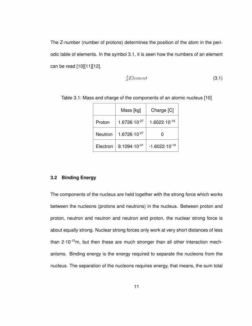
The Z-number (number of protons) determines the position of the atom in the peri-
odic table of elements. In the symbol 3.1, it is seen how the numbers of an element
can be read [10][11][12].
AZElement (3.1)
Table 3.1: Mass and charge of the components of an atomic nucleus [10]
Mass [kg] Charge [C]
Proton 1.6726·10-27 1.6022·10-19
Neutron 1.6726·10-27 0
Electron 9.1094·10-31 -1.6022·10-19
3.2 Binding Energy
The components of the nucleus are held together with the strong force which works
between the nucleons (protons and neutrons) in the nucleus. Between proton and
proton, neutron and neutron and neutron and proton, the nuclear strong force is
about equally strong. Nuclear strong forces only work at very short distances of less
than 2·10-15m, but then these are much stronger than all other interaction mech-
anisms. Binding energy is the energy required to separate the nucleons from the
nucleus. The separation of the nucleons requires energy, that means, the sum total
11

mass of nucleons is larger than the mass of the nucleus. As can be seen clearly in
Figure 3.1, the binding energy per nucleon in the heaviest atomic nuclei (e.g. ura-
nium) is about 7.5 MeV. It can also be seen that the binding energy per nucleon of
uranium is less than the binding energy per nucleon of medium-heavy atomic nuclei,
which corresponds to approximately 8 MeV (e.g, Fe-56).
Figure 3.1: Binding energy over Atomic mass number [10]
For example, if uranium is split into two medium-heavy atomic nuclei, the binding
energy per nucleon of the fission products is larger than the uranium nuclus binding
energy per nucleon. That means, energy must be released, as shown in Equation
12

3.2. In this equation both sides of the nuclear reaction equation, not only number of
nucleons but also energy must be conserved. It can also be seen that, in a fission,
not only energy, but also three new neutrons are released, which can then again
fission new uranium nuclei [10][11][12].
2352 U +1
0 n→9436 Kr +139
56 Ba+ 3 ·10 n+ 210MeV (3.2)
3.3 Mass Defect
According to Einstein’s theory of relativity E=m·c2, mass and energy are propor-
tional. This means that, on both sides of the nuclear reaction equation 3.2, not only
the same number of nucleons but also the same energy must be present. In in equa-
tion 3.2 with the atomic masses for: 235U=235,04392996amu, 1n=1,00866492amu,
94Kr=143,92295281amu ,139Ba=88,91763058amu and c=299 792 458 m/s, 1amu =
1,6605·-27 kg
∆m = mA(235U) +mA(1n)−mA(94Kr)−mA(139Ba)− 3 ·mA(1n) (3.3)
∆m = (235, 04392996−143, 92295281−88, 91763058−2 ·1, 00866492) ·amu (3.4)
∆m = 0, 21338354amu (3.5)
From this example, it is seen that energy must be released on the product side of
the equation 3.2 to satisfy the equation. On the other hand, it can also be seen that
13

the binding energy has a direct influence on the mass of atomic nuclei. The required
energy can now be determined by the theory of relativity [10][11][12].
∆E = 0, 21338354amu · c2 (3.6)
∆E = 210 MeV (3.7)
3.4 Neutron Reactions
In a nuclear reactor, many different neutron-nucleus nuclear reactions occur. In this
section, however, only the four most important reactions will be discussed.
• Neutron absorption with nuclear fission
• Neutron absorption with γ-ray emission
• Neutron elastic collision
• Neutron inelastic collision
Neutrons can be divided into two groups: thermal and fast neutrons. A fast neutron
has an energy of >1.0 MeV. In addition, the atomic nuclei can be distinguished into
fissile and non-fissile nuclei. Fissile nuclei include 235U and 239Pu. Non-fissile but
fissionable nuclei include 238U and 232Th. For the fission of an atomic nucleus, the
14
critical energy must be overcome. This results in the following condition for a fission:
Binding energy +Kin. Energy of the last neutron > Critical energy (3.8)
In the case of fissile atomic nuclei, the required critical energy is smaller than the
binding energy of the last neutron. In the case of atomic nuclei which are fission-
able, the binding energy of the last neutron is smaller than the critical enery at the
compound nucleus Therefore, the neutron kinetic energy must be larger then the
differnce, in order for fission to occur [10] [11][12].
15
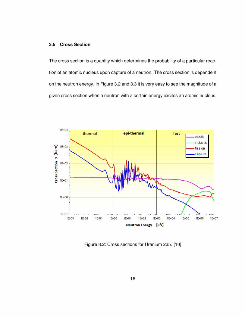
3.5 Cross Section
The cross section is a quantity which determines the probability of a particular reac-
tion of an atomic nucleus upon capture of a neutron. The cross section is dependent
on the neutron energy. In Figure 3.2 and 3.3 it is very easy to see the magnitude of a
given cross section when a neutron with a certain energy excites an atomic nucleus.
Figure 3.2: Cross sections for Uranium 235. [10]
16

Figure 3.3: Cross sections for Uranium 238. [10]
As can be seen clearly from the figures, a fission occurs at 235U even at low
neutron energies. For 238U, a certain neutron energy (velocity) is necessary to trigger
a fission or to improve the probability of a fission [10][11][12].
3.6 Moderation
The neutrons generated during nuclear fission have initial energies of approximatly
2 MeV and thus are fast neutrons. Since the fission cross section, is higher in the
17
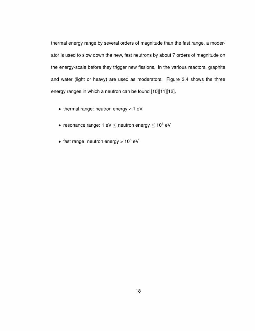
thermal energy range by several orders of magnitude than the fast range, a moder-
ator is used to slow down the new, fast neutrons by about 7 orders of magnitude on
the energy-scale before they trigger new fissions. In the various reactors, graphite
and water (light or heavy) are used as moderators. Figure 3.4 shows the three
energy ranges in which a neutron can be found [10][11][12].
• thermal range: neutron energy < 1 eV
• resonance range: 1 eV ≤ neutron energy ≤ 105 eV
• fast range: neutron energy > 105 eV
18
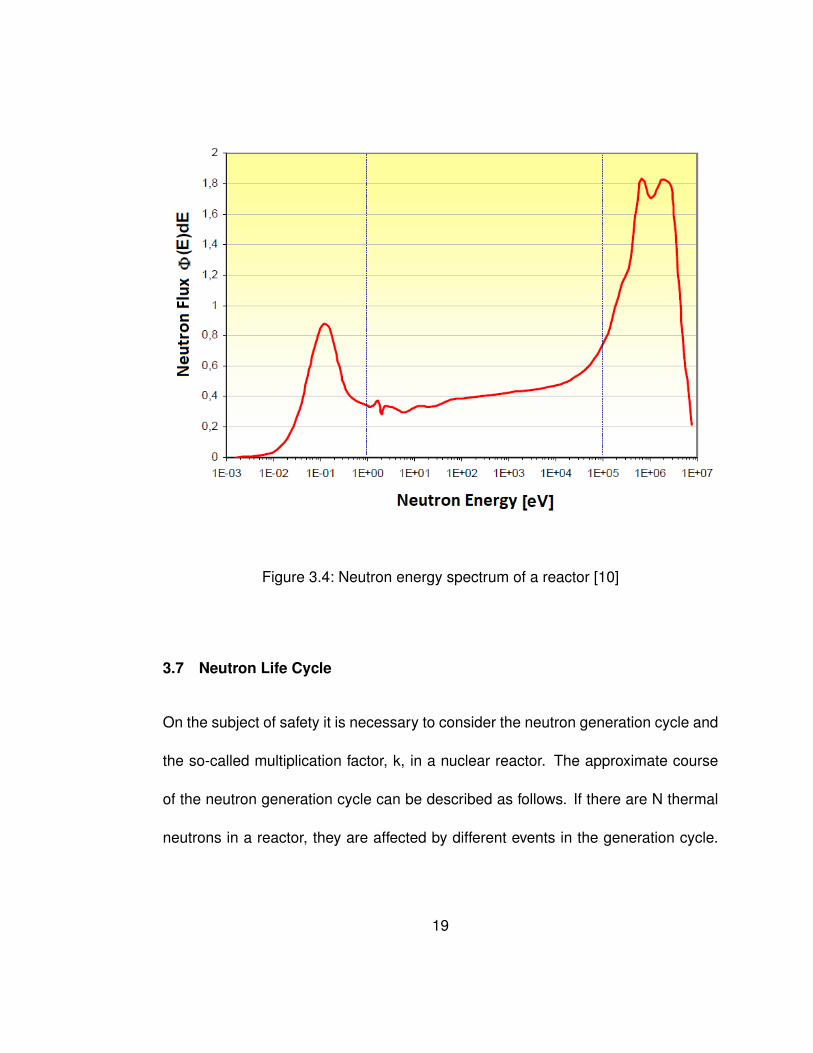
Figure 3.4: Neutron energy spectrum of a reactor [10]
3.7 Neutron Life Cycle
On the subject of safety it is necessary to consider the neutron generation cycle and
the so-called multiplication factor, k, in a nuclear reactor. The approximate course
of the neutron generation cycle can be described as follows. If there are N thermal
neutrons in a reactor, they are affected by different events in the generation cycle.
19
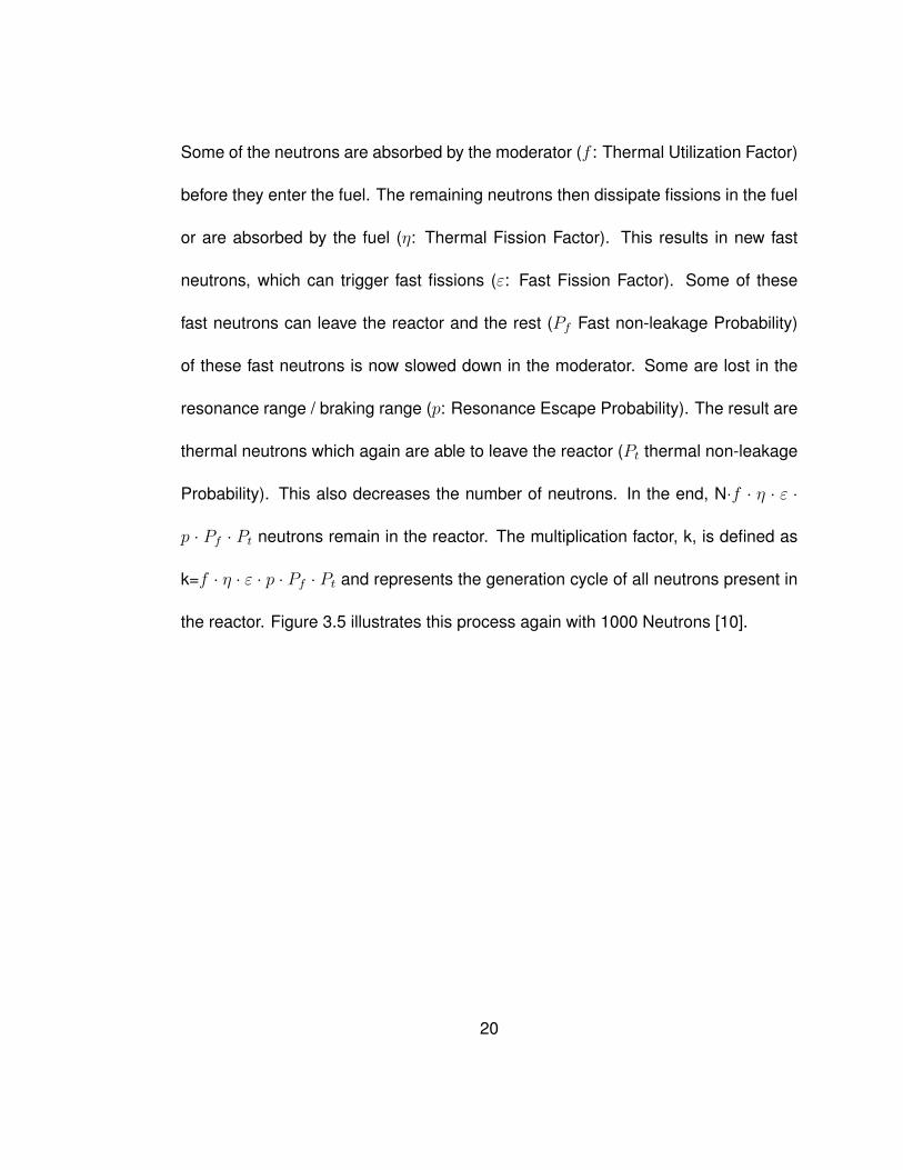
Some of the neutrons are absorbed by the moderator (f : Thermal Utilization Factor)
before they enter the fuel. The remaining neutrons then dissipate fissions in the fuel
or are absorbed by the fuel (η: Thermal Fission Factor). This results in new fast
neutrons, which can trigger fast fissions (ε: Fast Fission Factor). Some of these
fast neutrons can leave the reactor and the rest (Pf Fast non-leakage Probability)
of these fast neutrons is now slowed down in the moderator. Some are lost in the
resonance range / braking range (p: Resonance Escape Probability). The result are
thermal neutrons which again are able to leave the reactor (Pt thermal non-leakage
Probability). This also decreases the number of neutrons. In the end, N·f · η · ε ·
p · Pf · Pt neutrons remain in the reactor. The multiplication factor, k, is defined as
k=f · η · ε · p · Pf · Pt and represents the generation cycle of all neutrons present in
the reactor. Figure 3.5 illustrates this process again with 1000 Neutrons [10].
20
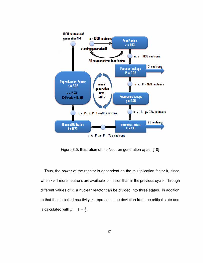
Figure 3.5: Illustration of the Neutron generation cycle. [10]
Thus, the power of the reactor is dependent on the multiplication factor k, since
when k > 1 more neutrons are available for fission than in the previous cycle. Through
different values of k, a nuclear reactor can be divided into three states. In addition
to that the so-called reactivity, ρ, represents the deviation from the critical state and
is calculated with ρ = 1− 1k.
21

• subcritical: k < 1, ρ < 0
• critical: k = 1, ρ = 0
• supercritical: k > 1, ρ > 0
At the various values of the reactivity (ρ), the power of the reactor may either rise
(ρ > 0), fall (ρ < 0), or remain at a steady level (ρ = 0). The neutron population is the
key factor for control and safety in the nuclear reactor. This is achieved by the control
rods in the reactor. The control rods are arranged between the individual uranium
fuel elements and can be retracted and extended as required. The control rods are
made of cadmium, boron or a similar material that has a high thermal neutron ab-
sorption cross section. Thus depending on how far the control rods are extended
or retracted into the core of the nuclear reactor, the multiplication factor, k, and the
reactivity, ρ, are influenced. In the same way the power of the reactor is influenced.
The energy released during nuclear fission is released as heat energy. This must be
transported through the various cooling cycles from the core to the turbine, where
it is finally converted into electrical energy via a generator. The control rods regu-
late the released energy and thus also the total electrical energy production of the
nuclear reactor [11][12].
22
4 Conventional Pressurized Light Water Reactors
Pressurized water reactors are the world’s most widely used types of nuclear power
plants. More than 70 percent of all nuclear power plants are designed as pressurized
water reactors. A pressurized light water reactor is a nuclear reactor type which uses
water as a coolant and as a moderator. As implied from the name of the reactor,
the used water is under high pressure, which has an effect on its thermodynamic
properties. In the case of light water reactors, normal water (H2O) is used as a
coolant, compared with deuterium in heavy water reactors. The rated power of a
pressurized water reactor is between 700 MWel and 1400 MWel. The most important
component of a pressurized water reactors is the reactor core in which the nuclear
reaction takes place. The core is made out of different fuel assemblies, some of
which are provided with control elements. The uranium enrichment (U235) of the fuel
in the fuel elements is between 1,9-4,8 percent. The fuel elements consist of the
approximately 4 m long fuel rods. The fuel rods consist, in turn, of one column of
fuel tablets consisting of sintered uranium dioxide (UO2). These fuel columns are
23
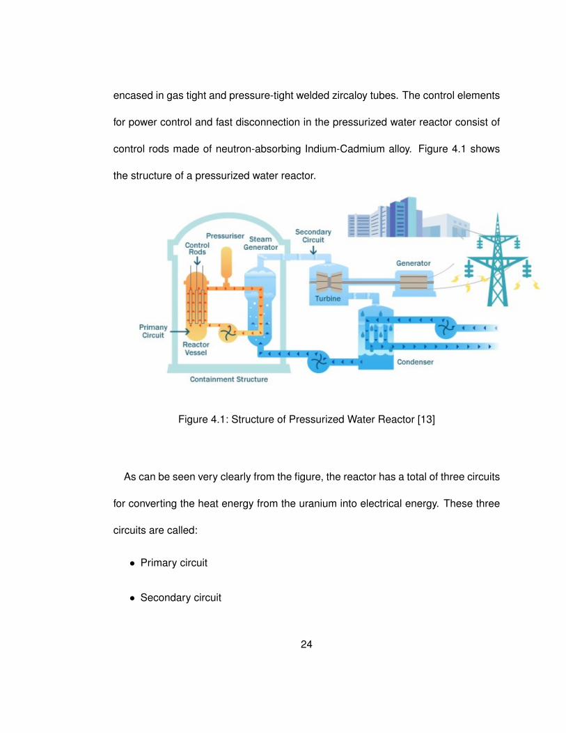
encased in gas tight and pressure-tight welded zircaloy tubes. The control elements
for power control and fast disconnection in the pressurized water reactor consist of
control rods made of neutron-absorbing Indium-Cadmium alloy. Figure 4.1 shows
the structure of a pressurized water reactor.
Figure 4.1: Structure of Pressurized Water Reactor [13]
As can be seen very clearly from the figure, the reactor has a total of three circuits
for converting the heat energy from the uranium into electrical energy. These three
circuits are called:
• Primary circuit
• Secondary circuit
24

• Cooling circuit
The primary circuit is located exclusively in a safety container. The separation of
primary and secondary cycle is the task of the radioactive contaminated water ex-
clusively within a safety container in the primary circuit. The advantage of this design
compared to the boiling water reactor is that no radiation protection measures are
necessary in the machine house where the turbines and the generator are located
[14][15][16].
4.1 Primary Circuit
The primary circuit consists of the reactor core vessel in which the uranium fuel rods
are located, the steam generators, the circulating pumps and connecting pressure
pipes between these components. The entire primary circuit is surrounded by a
protective cover made of reinforced concrete. The nuclear fission in the reactor core
vessel produces heat energy and thereby heats the cooling water of the primary
circuit. This heat energy is transported to the steam generator by means of the
pumps and the high pressure water. There, the heat energy is transferred to the
secondary circuit and the primary cooling water is thereby cooled. Afterwards, the
water is fed back into the reactor core and the process begins again. As already
mentioned, the water in the primary cycle is under a very high pressure of about 155
25
to 160 bar and has an evaporation temperature of 350◦C. Since only temperatures
of 290 to 325◦C are reached in the primary circuit, there is no phase change of the
coolant [10][14][15][17].
4.2 Secondary Circuit
The secondary circuit is a current clausius rankine power plant process. The water
pressure is increased by a feed water pump. Thereafter, the water is directed into
the steam generator, in which primary and secondary flow meet. There, the water
changes its aggregate state from liquid to gaseous. This steam now drives turbines
that are connected to a gernerator, which finally generates electrical energy. In the
turbines, the steam is expanded to a lower pressure and is passed into a further heat
exchanger in which the steam is again liquefied. The water is then returned to the
feed water pump and the process starts again. The secondary circuit is operated at
a pressure level of 60 to 70 bar. The evaporation temperature at these pressures is
about 280◦C. Thus, the pressure difference between primary and secondary side of
the steam generator ensures that the primary circuit, which is under high pressure,
triggers a phase change of the cooling liquid of the secondary circuit [10][14][15][17].
26

4.3 Cooling Circuit
The cooling circuit is used to ensure the liquefaction of the cooling water in the sec-
ondary circuit and to remove the waste heat which is not usable from the secondary
circuit. Cooling circuit and secondary circuit meet at the second heat exchanger.
For this last cycle, cooling water is required, depending on the location of the nu-
clear power plant, either from the sea or from a river. With the aid of a pump, the
cooling water enters the second heat exchanger of the secondary circuit and is sub-
sequently passed into the cooling tower. By this, it is then possible to dissipate the
waste heat, which is not usable, into the environment [10][14][15][17].
4.4 Power Plant Example
The following Table 4.1 shows technical data of a typical pressurized water reactor
as it is built around the world.
27
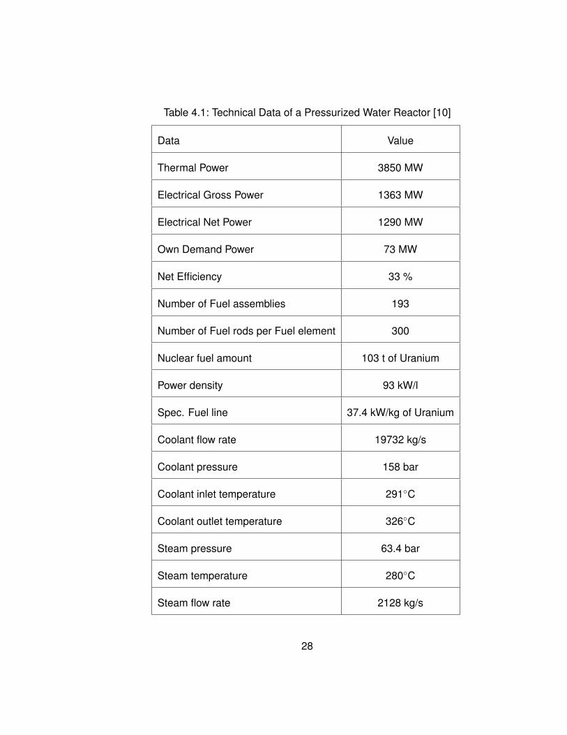
Table 4.1: Technical Data of a Pressurized Water Reactor [10]
Data Value
Thermal Power 3850 MW
Electrical Gross Power 1363 MW
Electrical Net Power 1290 MW
Own Demand Power 73 MW
Net Efficiency 33 %
Number of Fuel assemblies 193
Number of Fuel rods per Fuel element 300
Nuclear fuel amount 103 t of Uranium
Power density 93 kW/l
Spec. Fuel line 37.4 kW/kg of Uranium
Coolant flow rate 19732 kg/s
Coolant pressure 158 bar
Coolant inlet temperature 291◦C
Coolant outlet temperature 326◦C
Steam pressure 63.4 bar
Steam temperature 280◦C
Steam flow rate 2128 kg/s
28

Pressurized water reactors of this type are used worldwide and produce energy
for the industries and the population of the respective countries. Some examples
can be seen in Figure 4.2.
Figure 4.2: Locations of Nuclear Reactors worldwide. [18]
29

5 NuScale Systems
An example of a manufacturer of SMRs is the US-company NuScale. This enter-
prise is specialized in the design and development of integral pressurized water re-
actors (IPWRs). The company, founded in 2007, predicts that its technology will be
commercially available by the year 2025, and will contribute a large share to clean
energy generation [19][20].
5.1 NuScale Incorporated
The origins of NuScale Incorporated go back to the year 2000. That year the US
Department of Energy (DOE) funded the research and development of a SMR. Idaho
National Environment & Engineering Laboratory (INEEL) was commissioned with
the project, being supported by the Oregon State University (OSU), which was at
that time leading the development of passive safety systems and natural circulation
for nuclear power plant cooling. After completation of the research project in 2003,
the OSU scientists continued with the development of a SMR with natural circulation.
30

Finally they built a 1:3 version as a test facility for their design of a small modular
reactor. Following the construction of the test facility the scientists founded NuScale
in 2007. In exchange for a small equity in their new company they inherited related
patents from the university. In 2008, NuScale began the certification of its SMR at
the Nuclear Regulatory Commission (NRC). The design for the certification included
a 50 MWel module, which can be operated either independent or in cooperation
with other modules to generate electric energy and was thus the first company to
submit plans for a small reactor to the NRC. In 2011, NuScale employed 100 people
in three cities (Tigard, Oregon; Richland, Washington and Corvallis, Oregon). In
November 2014, NuScale announced that the first SMR nuclear power plant in the
United States will be located in Idaho and therefore submitted drafts to the Nuclear
Regulatory Commission in January 2017. If approved, the first facility with an SMR
system will be completed by 2026 [19][20].
31

5.2 NuScale Small Modular Reactor
A NuScale SMR is a integral pressurized water reactor that can operate as a stand-
alone unit or in a system of up to twelve SMR modules. All SMR units of the reactor
system are enclosed in a high-strength containment vessel and work in a common
pool filled with water, which contributes a great part to the safety of the reactors.
Each vessel is called module and is equipped with its own steam turbine-generator.
Figure 5.1 shows schematically how a NuScale SMR is constructed.
32

Figure 5.1: Schematic Construction of a NuScale SMR [19]
33

Due to the small size of the components of the reactor system compared to con-
ventional light water reactors, the reactor, pumps and turbines are easy to transport,
install and maintain. The NuScale SMR uses two cooling cycles to convert the heat
energy of the core into electrical energy through generators. Each module consists
of a reactor core, in which the fission reaction takes place. The reactor core is sur-
rounded by a high-pressure safety vessel which has a height of 13.7 m and a diame-
ter of 2.7 m and operates at a nominal operating pressure of 12.8 MPa. The reactor
containment vessel, with a height of 19.8 m and a diameter of 4.4 m, can withstand
pressures of up to 4 MPa without failing during accident scenarios. While the steam
generators are located in the upper part of the high-pressure safety vessel, the core
is installed in the lower part. Uranium oxide (UO2) with an enrichment of 5 % is used
as the fuel of the SMR in the core and is capable to produce 160 MWt power. The
primary cycle in the high-pressure safety vessel works according to the principle of
natural circulation, for this reason no pumps are needed to allow cooling water to
flow through the reactor core. The cooling water is heated by the nuclear reaction
as it crosses the core. By heating, the density of the cooling water decreases and
it rises upwards inside the closed cycle. As soon as the heated water reaches the
upper part of the high-pressure safety vessel, it flows through the steam generators
and is cooled there. The density of the cooling water increases again and is drawn
34

back by gravity to the bottom of the vessel. There it is again heated by the reactor
core and the process continues. The cooling water of the primary circuit is kept sep-
arate from the secondary circuit with the help of the steam generators in order to
prevent nuclear contamination of the pumps and turbines. The heat of the primary
circuit is transferred to the cooling water of the secondary circuit via the hundreds of
pipes in the steam generator. During this process, the secondary circuit coolant is
evaporated. The steam is used to drive turbines, which operate via a shaft to a gen-
erator which then produces electrical energy. After the turbines have been passed,
the steam loses its energy. The steam is liquefied again in a condenser and is then
pumped back into the steam generator with a feed water pump, where it begins
the cycle again. The high-pressure safety vessel and reactor comtainment vessel
comprises various design features that serve to increase safety and efficiency. On
the one hand, a vacuum is generated in the space between the two vessels, which
ensures that the pressure safety vessel does not have to be isolated. On the other
hand, the NuScale SMR has two passive safety systems which, in the event of an
accident, would lead to further cooling of the reactor. These two safety features are
called Decay Heat Removal System (DHRS) and Emergency Core Cooling System
(ECCS). Generally, the passive safety systems provide for cooling the core, using
natural convection, to remove the core decay heat when the normal feedwater sys-
35

tem is not available. Table 11.2 shows technical data of a NuScale SMR [19][20].
Table 5.1: Technical Data of a NuScale SMR
Data Value
Thermal Power 160 MW
Electrical Gross Power 50 MW
Dimensions 19.8 m x 4.4 m
Weight 700 t
Cost 5100 $/KW
Fuel 5.15 t of Uranium
5.3 Decay Heat Removal System
The decay heat removal system or short DHRS is one of the two passive safety
systems of the NuScale SMR. If the normal feedwater system of the secondary cycle
is not available, it is possible to cool the reactor using the DHRS. For this purpose,
capacitors, which are located on the outer wall of the high-strength containment
vessel, are used. It is also necessary to close the valves, which connect the steam
generators of the primary cycle to the secondary cycle, and to open the DHRS
valves. After opening, the cooling water of the DHRS cycle is able to transfer the
36

decay heat to the capacitors via the steam generators of the primary cycle. These
then give the decay heat to the pool, into which the entire reactor vessel has been
immersed. Natural convection also plays an important role in this process, since the
primary cycle is driven by this process. The DHRS is able to remove decay heat for
a minimum of 3 days without pumps or power. Figure 5.2 illustrates the discribeld
process of the decay heat removal system in a NuScale SMR works [19][20].
37

Figure 5.2: Decay Heat Removal System in a NuScale SMR [19]
5.4 Emergency Core Cooling System
The emergency core cooling system or short ECCS is the second passive safety
system of the NuScale SMR. If the normal feedwater system of the secondary cycle
38

or the decay heat removal system (DHRS) are not available, it is possible to cool the
reactor using the ECCS. In the head of the core reactor vessel, ventilation valves
are installed, which can be opened if necessary and thus lead to a pressure drop in
the core reactor vessel. It is also necessary to close the valves, which connect the
steam generators of the primary cycle to the secondary cycle. The cooling water
of the primary cycle begins to boil as a result of the pressure drop and changes
its state from liquid to gaseous when it passes throuth the core. The steam enters
the high-pressure safety vessel from the vent valves. Through the heat exchange
between the steam and the water of the reactor pool, the steam is again liquefied
and the core heat is released to the environment. The re-liquefied cooling water
collects in the lower area of the high-pressure safety vessel. When a certain level of
liquid has been reached in the high-pressure safety vessel the recirculation valves
which are installed on the sides of the core reactor vessel are opened. Through
these valves, the condensate returns to the vessel and passes through the core,
where it evaporates. Thus, the process can begin anew. This process makes use of
natural convection, since it also works without pumps. The difference to the natural
convection in normal primary cycle is that here a phase change of the cooling water
takes place. But in general, the driving force is the density difference in the different
phases of the process. Figure 5.3 illustrates the discribeld process of the emergency
39

core cooling system in a NuScale SMR works [19][20].
Figure 5.3: Emergency Eore Cooling System in a NuScale SMR [19]
5.5 Behavior of the Pool
As previously described, each reactor module of an SMR system is submerged in
a common pool of water. In this pool, there is water to cool the reactors in accident
scenarios for another 30 days after the incident. This is only possible if the water
pool is not refilled during this time, which is possible without any problems. For this
40

purpose, it is possible to use rotary pumps. One of the advantages of this design
is that the water needed for cooling is present at all times and does not have to
be first transported to the reactor. Furthermore, the pool is underground, which is
an advantage in terms of extreme events and offers significant protection against
earthquakes, floods, tornadoes and aircraft impacts. Figure 5.4 shows how the pool
behaves in the event of an accident. The figure shows the NuScale design to provide
long-term cooling (LTC) for the case of a complete station blackout without additional
cooling or water addition to the reactor water pool.
41

Figure 5.4: Pool Behavior in a NuScale SMR [19]
The figure shows the three phases of LTC defined in terms of heat transfer mech-
anisms. In addition, it shows how much heat is released from the reactor in the
different phases of the LTC. The first phase is called the water cooling phase. In
this phase of the LTC, the entire reactor is submerged in the water pool one of the
passive safety systems (ECCS/DHRS) would be in operation. The heat generated
in the core is then released via the containment vessel to the pool and thus the core
is cooled. If the pool is not cooled and no new water is introduced into the pool,
42

the liquid level will drop over time as a result of evaporation and subsequent satu-
rated liquid boiling in the pool. Estimates indicate that the liquid level of the pool has
reached the top of the containment vessel after about 3 days. It is also required that
at the end of the first phase of the LTC the released core heat is less than 1 MW
(thermal). In the second phase of the LTC, the liquid level of the pool is below the
top of the containment vessels and above the bottom of the containment vessels.
The second phase of the LTC of the reactor lasts from day 3 to day 30. At this
time, the reactor is cooled by the boiling water of the pool, which then evaporates in
time. Rough estimates suggest that all the water in the pool would evaporate after
30 days, without the addition of new water. At the end of the second phase of the
LTC, the core power should not exceed 0.4 MW (thermal) per module. The last and
third phase of long-term cooling of the reactor begins after 30 days. After this time,
it is sufficient to cool the reactor by the natural convection with the surrounding air
and the heat radiation from the outer surface of the containment vessels. The core
heat at this time is only 400 kW per module [19][20].
43

6 Advantages of Small Modular Reactors
Small modular reactors are a further development of the old conventional nuclear
reactors, which have already been built for decades. Through new technologies
and innovations, SMRs have many advantages over the conventional large nuclear
reactors. For example, light water reactors with an electrical output of 1400 MW with
integral pressurized water reactors of 50 MW can be compared with one another.
The advantages of the SMRs include:
• Size
• Transportation
• New Applications
• Manufacturing Process
• Safety
These points are among the most important advantages and will be further dis-
cussed for this reason [1][2][10][17][19].
44

6.1 Size
The difference in size is one of the main reasons why SMRs have an advantage
compared to typical conventional reactors. The dimensions of a conventional reac-
tor, such as is built for example in the United States of America, are 61 m x 37 m.
In comparison, the dimensions of a NuScale SMR are only 19.8 m x 4.4 m. Thus,
the conventional reactor is about 217 times larger than the SMR. The advantages
due to size are unambiguous. On the one hand, the SMR does not need a separate
building to work, for example, it can simply be placed next to the machine, which
is to supply it with power. On the other hand, the energy losses that occur during
the transport of the energy are eliminated since the SMR has to work locally and no
large distances have to be bridged [1][2][10][17][19].
6.2 Manufacturing Process
Each conventional nuclear reactor is individually planned, licensed, tested and sub-
sequently built, with great effort in a building. This building has to be planned and
licensed after special conditions for nuclear power plants. This process makes the
core actuator very expensive. Compared to small modular reactos which can be built
on the assembly line at significantly better costs. In addition, SMRs can be manu-
factured in one place and mounted in a different location. This is made possible the
45
smaller size and by the use of standardized components. This also eliminates the
strict licensing procedures by authorities for each individual reactor since SMRs are
all the same. The production of spare parts is also simpler and cheaper for small
modular reactos, thanks to the use of standardized components. If a component
is no longer working, it can be quickly replaced by a new component of the same
type and does not have to be produced anew. For these reasons, it is very easy to
derive the economic benefits of small modular reactors in terms of manufacturing
[1][2][10][17][19].
6.3 Transportation
Another advantage of the small modular reactors is that they can be transported
easily. This is made possible by the low weight and the demountability of the SMRs.
In some regions of the world, it is difficult to produce energy or transport energy to
these regions. Examples include islands in open Pacific Ocean, deserts or states
where the energy grid is poorly developed. Due to the transportability of the small
modular reactors it is also possible to supply these regions of the earth with suffi-
cient energy. The individual parts of the reactors can be transported by ship, truck
or plane to the respective continent, mounted there and then provide the energy
supply. Thus, in the future it will be possible to supply every part of the earth with ef-
46

ficient cheap and clean energy. In special cases, submarines or rockets can also be
used to transport the reactors to power a space station or an underwater laboratory
[1][2][10][17][19].
6.4 New Applications
In addition, new applications for nuclear reactors are possible with small modular
reactors. Large conventional light water reactors have hitherto only been used to
generate large scale energy for large cities, densely populated regions and aircraft
carriers. In other words, only where there is enough space to build a large reactor.
In addition to that a large body of water has to be near the conventional nuclear
power plant due to it large decay heat. Due to the considerably smaller size of
an SMR, machines or small regions whose energy requirements are not so high
can be supplied in the future. Examples of this are tunnel boring machines, large
production plants or countries in Africa whose energy requirements are generally
very low. Another factor for these new applications is the lower price of a small
modular reactor compared to a conventional reactor [1][2][10][17][19].
47

6.5 Safety
Small modular reactors are safer than conventional pressurized water reactors due
to their passive safety systems. One of the most important features of the pas-
sive safety of an SMR is the natural convention cooling cycle which continues to
function even in the event of power or secondary systems failing, to cool the nu-
clear core of the reactor. In addition, the reactor core of the SMR is surrounded
by several safety vessels and the entire reactor is placed in a water pool below the
ground level. If an accident occurs during which the pool is completely emptied by
the passive safety systems, but the reactor still needs to be cooled with water, the
pool can be easily refilled with mechanical pumps and the cooling process can be
continued[1][2][10][17][19].
48

7 Nuclear Energy Cycle
This chapter deals with the nuclear energy cycle in short how the released heat
energy of the uranium is transferred into electrical energy. For this purpose, the
primary topic of this chapter is the secondary cycle of a steam-electric power plant.
The task of a power plant is to convert primary energy into electrical energy. It is
a thermal power plant when the primary energy is first converted into heat energy
and then transferred to a heat engine. Each thermal power plant consists of a heat
generator and the heat engine. The heat generator converts the primary energy of
the power plant into heat and the heat engine converts this heat into useful electrical
energy. Depending on what primary energy a thermal power plant uses, it can be
divided into three different types.
• Fuel power plants (Coal and Gas)
• Nuclear power plants
• Thermal Solar power plants
49

In the heat engine, the working fluid passes through a cycle and is heated. At a
special point in the cycle, this heat is transferred to the secondary cycle via a steam
generator. As a working medium water or steam is almost always used, due to its
good thermodynamic properties and high heat capacity. The secondary cycle of a
steam-electric power plant is commonly referred to as Rankine cycle and is named
after the Scottish engineer William John Macquorn Rankine. The Rankine cycle is
generally used for any type of power plant where steam is used to generate energy.
The Rankine basic cycle can be divided into four primary components.
• Feed Pump.
• Steam Generator
• Steam Turbine
• Condenser
The construction scheme of the cycle can be seen in Figure 7.1.
50

Figure 7.1: Construction scheme of the Rankine cycle [21]
It is also possible to divide the rankine cycle into an ideal and a real cycle. The
difference lies in whether or not the feed pump and the steam turbine are considered
as ideally working components [22][23][24].
51

7.1 Ideal Cycle
Figure 7.2 shows a Temperature-Entropy-diagram of an ideal Rankine cycle. As can
be seen from this figure the cycle runs as follows.
Figure 7.2: T-S-diagram of an ideal Rankine cycle [21]
• 1-2, adiabatic isentropic pressure increase by the feed pump
• 2-3, isobaric heat supply and superheating in the steam generator
• 3-4, adiabate, isentropic expansion of the steam in a steam turbine
• 4-1, isobaric condensation of the vapor in the condenser
52

When the first state is reached again, the cycle begins again. At the beginning of
the ideal cycle (point 1), there is a liquid working medium that is compressed to a
high pressure with the feed water pump (point 2). The pump has to do work, but
this is done by the later expansion of the steam in the turbine. After the pressure
increase, the working medium is directed into the steam generator, where it changes
its state of aggregation. In this process, three subprocesses occur. First, the working
medium is heated to the boiling point (point 2*) then it is evaporated (point 2**)
and finally brought into a superheated state by further heating of the now vaporous
working medium (point 3). The steam is now expanded in the steam turbine, while
doing work and releases mechanical energy. With this mechanical energy on the
one hand, the feed pump, but also the electric generator for power generation is
operated. The working medium is partially condensed during this process (point 4).
Subsequently, the remaining vapor is liquefied again in the condenser so that the
working medium again assumes its initial state (point 1). After that the medium is
again passed into the feedwater pump. The work done can be read directly from
the T-S diagram. The area enclosed by the working curve of a cycle represents the
work gained during the cycle. In order to be able to quantitatively evaluate the work
achieved, the efficiency (η) of the cycle has to be considered. The efficiency of an
ideal Rankine Cycle is defined as follows.
53

ηrevth =wrev4−3 − wrev2−1
q3−2=wrevt
q3−2(7.1)
From the given work of the turbine (w4-3), the required work of the feedwater pump
(w2-1) has to be deducted in order to determine the net work (wt) of the process. The
advantage of the rankine cycle is the large specific cycle work that results from the
high specific volume difference between liquid and vapor. As a result, the feed water
pump has to do little work to increase the pressure, while the turbine generates
significantly more work in the expansion of the working fluid. This leads to relatively
high efficiencies of up to 40 %.To calculate the efficiency level, extensive tables of
the performance of the working fluid at different pressures and temperaturesare are
required [22][23][24][25].
7.2 Real Cycle
In the real Rankine cycle, the feed water pump and the steam turbine are not working
ideally. Now these components have an inner efficiency like the rest of the process.
This means that not all the work that these components require is converted. Part
of the work involved in operating the feed water pump and the steam turbine is lost
inside these components. The losses can be seen in the following T-S diagram 7.3
with an increase of the thermodynamic value entropy.
54
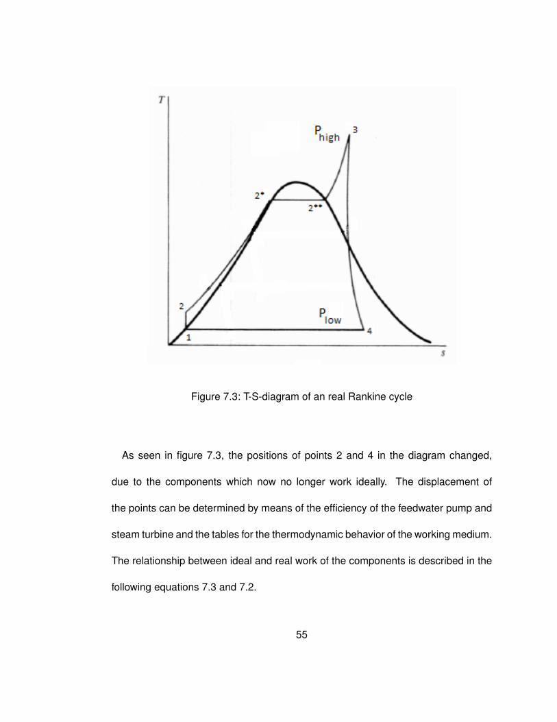
Figure 7.3: T-S-diagram of an real Rankine cycle
As seen in figure 7.3, the positions of points 2 and 4 in the diagram changed,
due to the components which now no longer work ideally. The displacement of
the points can be determined by means of the efficiency of the feedwater pump and
steam turbine and the tables for the thermodynamic behavior of the working medium.
The relationship between ideal and real work of the components is described in the
following equations 7.3 and 7.2.
55

wtur = wrevtur · ηtur (7.2)
wpum =wrevpum
ηpum(7.3)
It can be clearly seen from the equations that the feedwater pump requires more
work in non-ideal behavior to bring the working fluid to the desired pressure and the
steam turbine produces less work for the cycle in non-ideal behavior than in ideal
behavior. The reason for this is that the losses during operation of the components
are expressed as heat losses, friction, and in refluxes of the fluid via the blades in
the feedwater pump and the steam turbine. The heat and the fluid refluxes have
an influence on the working medium and change the thermodynamic properties of
the working medium. Among other things, the heat increases the specific volume
of the fluid and the refluxes increase the mass of the working medium. The feed
water pump must now compress a higher volume resulting in a higher workload and
thus a lower efficiency. For turbines on the other hand more volume is available for
expansion due to the higher specific volume and thus more work can be generated.
As a result of these processes, the surface area of the area enclosed by the working
curve of the cyclic process and thus also the work won and efficiency change. All
this can be seen from Figure 7.2 and in Figure 7.3 [22][23][24][26].
56
7.3 Optimization
The rankine cycle can be improved by various operational and design steps. These
steps can not only gain more work but also increase the efficiency of the entire cycle.
One of the operational steps is the increase in steam parameters. So the increase
of temperature and pressure at the highest point of the cycle. Constructive steps
include reheating and regenerative feedwater preheating [23][24].
7.3.1 Reheating
The maximum temperature increase is limited by the thermal capacity of the compo-
nents, thus an increase in efficiency by increasing the steam parameters is limited.
Reheating can circumvent this fact. In this process the steam is first expanded in a
high pressure turbine to an intermediate pressure and then redirected to the steam
generator. There the steam is overheated again and is then expanded in a low
pressure turbine to the condensation pressure. Due to the reheating, the average
temperature of the heat supply increases and thereby raises the temperature level
of the steam in the steam generator. The energy loss during heat transfer from the
heat generator to the heat engine is reduced. The effects of reheat are shown in
Figure 7.4 in a T-S diagram. The reheat increases the overall efficiency of the cycle
by about 10 % [23][24].
57

Figure 7.4: T-S-diagram of an Rankine cycle with Reheating
7.3.2 Regenerative Feedwater Preheating
Another way to increase the efficiency results from the preheating of the feedwa-
ter. In this process, a portion of the steam is removed from the turbine and used to
preheat the liquid working medium. In the turbine enters a certain amount of steam
which is expanded from a high pressure to an intermediate pressure, the so-called
extraction pressure. Now, part of the steam is taken out of the turbine and fed to
the feedwater preheater, while the remaining steam is expanded to the condensa-
tion pressure. The extracted steam transfers its heat energy to the liquid working
medium and thus increases its temperature. The extracted steam condenses in the
58

preheater and is then mixed with working fluid, which has been liquefied by the con-
denser. The feedwater preheat increases the temperature level of the steam in the
steam generator and heat transfer losses are reduced. The effects of a regenerative
feedwater preheater are shown in Figure 7.5 in a T-S diagram [23][24].
Figure 7.5: T-S-diagram of an Rankine cycle regenerative Feedwater preheating
7.4 Nuclear Cycle
In the nuclear energy cycle, the heat generator is the core in which uranium is fis-
sioned and thus energy is released in the form of heat. This heat is transported to
the heat engine via the primary cooling circuit. The circuits are connected to each
other via the steam generator in which the heat transfer from the heat generator to
the heat engine takes place. Since this heat engine cycle is in a steady state during
59

operation of the nuclear power plant it can be assumed to be thermodynamic and
not thermal-hydraulic as is the case with the primary cycle. Since nuclear power
plants operate in comparison to other steam power plants only at a low temperature,
the efficiency for this type of energy production is limited. The cycle of the heat en-
gine must be adapted to these conditions, as high pressures and high temperatures
are not possible. Superheating of the steam is limited, as a result of which the ex-
pansion of the steam in the steam turbine proceeds almost completely in the vapor
curve. The great advantage of nuclear energy compared to other energy sources is
the high energy density of uranium in the core. This surpasses fossil fuels by several
orders of magnitude. For example, the energy density of hard coal is 34 MJ/kg as
compared to the energy density of Uranium-235 at 79.39·106 MJ/kg. A disadvan-
tage of the use of nuclear energy are the radioactive fission products.
Exposure to radiation must be reduced by very complex safety systems. In the
event of an accident, no radioactive substances or radiation are released into the
environment. Consequently, a nuclear power plant emits far less radioactivity than
for example a coal power plant as coal contains natural radioactive isotopes that
enter the environment from combustion. In addition a nuclear power plant produces
no greenhouse gases including CO2, SO2 or N2O [10][22][23][24].
60
8 Programming in RELAP 5
RELAP is an abbreviation for Reactor Excursion and Leak Analysis Program and
is usually used for the simulation of the thermal-hydraulic behavior of the reactor
coolant system and the core for various operational transients and postulated acci-
dents that might occur in a nuclear reactor.
RELAP uses so called "cards" for the simulation of the models. Each card contains
a special order: what the program has to do or under what conditions the program
should run. For example, the card with the number 0000100 contains the name of
the project and what kind of problem (steady state or transient) is simulated. With
the help of these cards, every component of the system is modeled. Each new card
implements a new part of the system. For example: a pipe, a pump, or other compo-
nents for a thermal-hydraulic simulation. There are several cards, all with a different
orders of how the new component is modeled, and under what conditions.
The modeling of a new componet starts with the card XXX0000. This card imple-
ments the name of the new component and what kind of component is modeled.
61

The XXX stands for the component number which is a variable, but a system of
numbers would be an advantage. A system of numbers is especially important for
very large systems, because otherwise the overview of the simulated system is very
quickly lost. After naming the component, it is split into a chosen number of cells for
a more exact modelling. Each cell contains a length and volume which is also cho-
sen with a special card of RELAP. There are several other options for the cells, for
example: height, angle, and roughness which are also very important for complex
simulations. The most important thing about modeling components is that the com-
ponent number and command number on the cards match. Otherwise an already
finished component can get a new boundary condition, which with RELAP cannot
work. With numbers for XXXYYYY, every card works. While XXX, as already said
stands for the component number, YYYY is the command number for every simu-
lated cell of the component. In addition to that, the temperature, the pressure, and
the boundary conditions of the fluid inside each cell have to be chosen. Also, for this
RELAP has special cards which have to be used. All modeled components can be
connected to each other at so called "junctions". These also have to be modeled
with RELAP cards like the modeled components. With the help of the junctions, it is
possible for RELAP to simulate very complex systems of components. For example,
a light water reactor, SMRs or any other thermal-hydraulic system, for very simple
62

problems, like the "Edward’s Pipe Problem", single junctions are not necessary, be-
cause it deals with only one componnent, which is not conected to anything else. A
junction can be used to create a hole in the last cell of pipeline or any other com-
ponent of the system. For example, the junction is modeled as a valve that can be
opened and closed.
The following figure shows the beginning section of a RELAP code. The code shows
how the cards are called and how certain commands are executed. It will only be
clarified here how RELAP 5 is programmed [27][28][29][30][31].
63

Figure 8.1: Scheme of RELAP 5 simulation. [31]
After modelling the components for the chosen system or the chosen problem
the code has to be input in RELAP. For starting RELAP, a bat-data was written to
execute the RELAP5 program with the right input data. This input data is the written
code. For example the "Pipe blowdown Problem" . Before the start of the simulation,
RELAP checks the code for mistakes, and will not start until every line is correct. If
the code is correct, RELAP will start the simulation. It starts with calculating the
64

steady state for the chosen system, or the chosen problem, until everything is in
an equilibrium. After that, RELAP runs the code under the given boundaries and
parameters. After RELAP has finished its simulations, it saves the data in three files.
One file shows how RELAP has done the simulation, and also contains all simulation
errors. The second file is the plot file, which contains all measurement data. This
file has to be opened by a special software, called "AptPlot" . This software is able
to read the binary file and can create plots for the evaluation. Although, the plot was
made in another software, called "Origin" , because this program is specialized to
create very complex and exact plots [27][28][29][30][31].
65
9 Thermal-hydraulics in RELAP 5
RELAP 5 uses mathematical models to analyze operational and accident scenarios
that can occur in a nuclear fission-based power plant. With RELAP 5, it is possible
to describe the physical processes that take place in a nuclear power plant and to
analyze and evaluate them at the end. As a model, RELAP 5 uses a set of partial
differential equations that can describe and predict certain phenomena in a range of
applicability. The prediction capability of the models can be considered as a com-
pelling criterion, because the set of partial differential equations can only describe
and evaluate certain scenarios.
The general solution of this set of partial differential equations is very complex and
very difficult to solve. An analytic solution of the nonliniear partial differential equa-
tions is generally not possible. The most commonly used approach to solving partial
differential equations is discretization, thus solving a discretized version of the sys-
tem.
RELAP 5 simulates the thermal-hydraulic behavior of water and steam in the power
66

plant cycles for the transport of energy generated in the reactor. Despite the benefits
of the discrete solution of these systems, some problems with this type of solution
must be considered. The solution of discretized equations is subject to errors that
must be monitored and solution steps controlled to reduce. Moreover, the interpre-
tation of the results is a more notable problem. It should be noted that RELAP 5 is
a mathematical model that is based on physics models to simulate nuclear power
plants. As a starting point for the thermal-hydraulic calculations of the systems sim-
ulated in RELAP 5, the following space-time-dependent partial differential equations
are considered.
• Conservation of Mass
• Conservation of Momentum
• Conservation of Energy
The nomenclature used hereinafter can be found in the appendices in chapter 15
[32][33][34][35].
67

9.1 Conservation of Mass
∂
∂t(αkAρk) +
∂
∂x(αkAρkυk) = AΓk
(9.1)
9.2 Conservation of Momentum
∂
∂t(αkAρkυk) +
∂
∂x(αkAρkυ
2k) = −αkA
∂P
∂x+ αkρkBxA
− αkρkA FWkυk + AΓkυi − αkρkA FIk(υk + υk′)
− Cαkαk′ρmA[∂
∂t(υk + υk′) + υk′
∂υk∂x− υk
∂υk′
∂x
](9.2)
68

9.3 Conservation of Energy
∂
∂t(αkAρkuk) +
∂
∂x(αkAρkukυk) = −AP ∂αk
∂t− P ∂
∂x(αkAυk)
+ AQwk + AQik + AΓikh∗k + AΓwkh
′k + A DISSk
(9.3)
The model represented by these partial differential equations is called a two-fluid
model. In this model, each phase (liquid or gaseous) is considered separately and
for each phase one of the conservation equations can be established. The model
evaluates, compared to other models, thermal-hydraulic non-equilibria between the
different phases by its basic equations. As a result, the two-fluid model is precise
and can easily solve and evaluate thermal-hydraulic problems very precisely. In
general, for the two-fluid model, it can be said that each phase has its own velocity,
temperature and pressure. While the different velocities of the phases are caused
by density differences, temperature differences between the phases are generally
caused by the time delay of the energy transfer between the phases. The pressure
difference of the different phases of the two-fluid model is generated by three effects:
• pressure differences due to surface energy of a curved interface
69

• pressure differences due to mass transfer
• pressure differences due to dynamic effects
The first effect is generally caused by the phases, since the simple existence of
an interface results in a pressure difference from the total mechanical equilibrium
between these phases. The second effect is caused by large mass flows between
the phases due to phase change (high evaporation or condensation) at the interface.
Due to the dynamics in which phase A has a greater pressure than phase B due
to very rapid energy deposition or pressurization effects, the third effect is finally
produced.
In most cases, however, it can be assumed that the pressure in the phases is the
same and thus there are no pressure differences. RELAP 5 takes this case in its
calculations. From RELAP 5 manual volume 1 "the phasic pressures are assumed
equal" [27]. Thus it is assumed:
P = Pf = Pg (9.4)
A counter example, in which pressure differences are important is in research
on explosive boiling. In these cases, a local momentum equation (e.g. Rayleigh
momentum equation) is used to model the pressure difference of the two phases.
Furthermore, it can be seen from the equations 9.1, 9.2 and 9.3 that the phases
70
of the model are connected with each other via different parameters. Two of these
values are Γk and Γ′k. Γk and Γ′k represent the mass transfer rate due to the phase
change and the interaction force between the different phases. It can be assumed:
Γk = −Γk′ (9.5)
The model provides for dividing the mass transfer rate Γk into two different areas.
On the one hand, the mass transfer rate at the interface between vapor and liquid in
the mass of the fluid Γik is considered. On the other hand, the mass transfer rate at
the interface between vapor and liquid near the walls Γwk is considered.
Γk = Γik + Γwk (9.6)
71

Figure 9.1 shows the scheme of the model in terms of mass transfer rate Γk.
Figure 9.1: Mass transfer rate in RELAP 5 [27]
The expression of the momentum equation in RELAP 5 is reduced to Bernoulli
equations for a steady, incompressible and frictionless flow. The reason for this is
that impulse effects in the reactor safety analysis are regarded as secondary com-
pared to mass and energy conservation. It follows that a less accurate formulation
(compared to mass and energy conservation) is acceptable, especially since there
72
are large momentum sources and sinks (pumps or turbines) in nuclear reactors. The
reason for using the momentum equation in extended form is that it has made the
development of the RELAP 5 numerical scheme easier. The force terms on the right
sides of the equation 9.2 are:
• αkA∂P∂x
= pressure gradient
• αkρkBxA = body force
• αkρkA FWkυk = wall friction
• AΓkυi = momentum transfer due to interface mass transfer
• αkρkA FIk(υk + υk′) = interface frictional drag
• Cαkαk′ρmA[∂∂t
(υk + υk′) + υk′∂υk∂t− υk ∂υk′∂t
]= force due to virtual mass
The term FWk belongs to the frictional resistance of the walls through which the
fluid flows and is a product of different friction coefficients. The coefficient FIk is part
of the frictional resistance of the interface between the vapor and the liquid phase of
the fluid. For the calculation of FIk two different models are used (drift flux and drag
coefficient), depending on whether the flow is a laminar or a turbulent flow.
The listed virtual mass term is simplified in the RELAP 5 encoding. It follows that the
spatial derivative part of the expression is neglected in the calculations. The reason
73

for this simplification is that numerical computation of the spatial derivative part of the
expression can lead to inaccuracies, which can then lead to nonphysical properties
in the numerical solution. The coefficient of the virtual mass in turn depends on
the type of flow and is assumed in RELAP 5 as C>0,5. A C-value greater than 0,5
is suitable for bubbling or dispersed flows, unlike separate or stratified flows where
a C-value of 0 is appropriate. The primary effect of the virtual mass term is the
mixing sound velocity of the liquid-vapor fluid. Thus, it is acceptable that in the
RELAP 5 model the simplified form is used . As seen in the next equation, 9.7,
the conservation of momentum at the transition between phases requires that the
values that participate in the momentum exchange add up to zero.
ΓkAυik − (αkρkA) FIk(υk − υk′)− Cαkαk′ρmA[∂
∂t(υk − υk′)
]− Γk′Aυik′ − (αk′ρk′A) FIk′(υk′ − υk)− Cαk′αkρmA
[∂
∂t(υk′ − υk)
]= 0
(9.7)
The equation shows that all spatial derivatives of the momentum conservation
have been removed, as described above. This special interface momentum balance
results from the conservation of momentum for the different phases in equation 9.2.
74

In addition, for equation 9.7, it is assumed that the interfacial impulse transfer due to
friction and due to the mass transfer add independently to zero.
The energy conservation equation represents the temporal and spatial evolution of
energy in the simulated two phase system of RELAP 5. In the equation, the following
simplifications are surpassed:
• Reynolds heat flux is neglected
• interfaces energy storage is neglected
• internal phasic heat transfer is neglected
In energy conservation as well, as in mass transfer, a differentiation is made be-
tween energy transfer near the wall and energy transfer in the fluid. The values Qwk
and Qwk′ are heat transfer rates of the phases near the walls of the system. Qw
represents the total heat transfer near the walls of the system, as shown in equation
9.8.
Qw = Qwk +Qwk′ (9.8)
The specific enthalpies h∗k and h∗k′ are related to the mass transfer between the
different phases in the fluid region and the specific enthalpies h′k and h′k′ are in turn
related to the mass transfer between the different phases around the walls of the
75
system. Thus it is again distinguished whether the mass transfer and the resulting
energy transfer occurs near the walls or in the fluid. As already discussed, the phase
transition of the fluid consists of two parts. On the one hand the phase transition in
the area of the fluid (Γik) and on the other hand the phase transition in the area
of the walls (Γwk) of the system. Each phase change also includes heat transfer
effects, which can also be differentiated, depending on whether the heat transfer
takes place in the fluid (Qik) or near the walls (Qwk). For the energy exchange
between the phases due to heat or mass transfer, it is necessary that this results in
a total of zero, as clearly shown in equation 9.9.
Qik +Qik′ + Γik(h∗k − h∗k′) + Γwk(h
′k − h′k′) = 0 (9.9)
The values for the heat transfer between the phases (Qik & Qik′) can also be
divided into two parts. On the one hand in the heat transfer (QBik & QB
ik′) in the
fluid and on the other hand in the heat transfer near the walls (QWik & QW
ik′). The
interphase heat transfer can be seen as shown in Figure 9.2. In addition, the total
heat transfer between the phases can be expressed by equation 9.10.
76

Figure 9.2: Heat transfer in RELAP 5 [27]
Qik = QBik +QW
ik (9.10)
The heat transfer between the phases in the fluid occurs at the interface between
the phases. The heat transfer takes place at the saturation temperature TS and the
total pressure P . In the equation for the interface heat transfer Hik represents the
interface heat transfer coefficient and Tk is the temperature of the phase.
77
QBik = Hik(Ts − Tk) (9.11)
Furthermore, it is assumed that the values of equation 9.9 on wall and between
phases sum independently to zero. This can be seen from the next equations 9.12
and 9.13.
Hik(Ts − Tk) +Hik′(Ts − Tk′) + Γik(h∗k − h∗k′) = 0 (9.12)
QWik +QW
ik′ + Γwk(h′k − h′k′) = 0 (9.13)
In order to determine the mass transfer rate near the walls, QWik = 0 is assumed
for phase transitions from phase k to phase k′ and QWik′ = 0 for phase transitions
from phase k′ to phase k. With the equation 9.13 and these assumptions, the mass
transfer rates for the phases on the wall are:
Γwk =−QW
ik
(h′k − h′k′)(9.14)
Through this new expression in equation 9.15 and equation 9.11, the equation
9.10 can be expressed in a new general form:
Qik = Hik(Ts − Tk)−Γwk
(h′k − h′k′)(9.15)
78
The last value of the energy conservation equation is the phasic energy dissipation
term DISSk. DISSk represents the sum of the energy dissipation effects through
pumps, turbines or wall friction in the system. Equation 9.16 is shows how the phasic
energy dissipation term expresses for wall friction losses. Dissipation effects due to
mass transfer between the phases, friction between the phases, or virtual mass are
neglected because these are very small in the energy conservation equation.
DISSk = αkρkFWυ2k (9.16)
The losses of the different phases can be summed up again to a total value, as
can be seen in equation 9.17.
DISS = DISSk +DISSk′ (9.17)
As can be seen from these equations and the made assumptions, the description
of the model that RELAP 5 uses is very difficult, and it is very clear that the phases
and the system are interconnected and interact with each other through these partial
differential equations [27][32][33][34][35].
79
10 Natural Circulation
In conventional nuclear power plants, the circulation of the coolant of the primary
cycle and the secondary cycle is operated by reactor coolant pumps or by feedwater
pumps. The NuScale SMR uses the natural circulation of water in its primary cycle
to dissipate its core heat. The natural circulation is generated exclusively by the
arrangement of the core (heat source) and the steam generator (heat sink). Natural
circulation, in comparison to the principles of conventional circulation methods, has
the advantage that no external energy is needed to maintain the cycle. This is a
particularly strong safety aspect of a NuScale small modular reactor. This chapter
deals with the physical principles of natural circulation [19][36][37][38].
10.1 Physical Principle
The driving force of natural circulation is the density difference of the fluid present
in the system. These density differences in the fluid are produced by heat removal
on one side and heat supply on the other side of the circuit. The density differences
80

result in a pressure difference in the system, which is also referred to as the driving
pressure. In the following equation 10.1, the pressure difference generated by the
different densities is shown.
∆p = h · g · (ρ2 − ρ1) (10.1)
As can be seen very clearly from the equation, the pressure difference depends
only on the height to be overcome, as well as the temperature at heat source and
heat sink, which leads to the density difference in fluid. By this pressure difference,
the heated fluid flows from the heat source to the heat sink. When the natural
circulation comes to a closed circuit, there is talk of gravity circulation. With gravity
circulation, it should be noted that the heat source must be located lower than the
heat sink in the circuit. This is one of the prerequisites that the cycle needs to work.
As the fluid enters the heat source its density decreases. As a result, it rises by
static buoyancy in a gravitational field up to the heat sink. At the heat sink heat is
removed from the fluid, which leads to a decrease in temperature and thus to higher
density. The denser fluid now sinks from the heat sink to the heat source and the
cycle begins again. Figure 10.1 illustrates again the mode of operation of the natural
circulation.
81
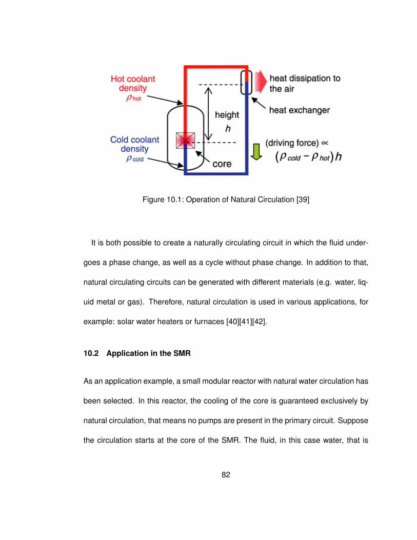
Figure 10.1: Operation of Natural Circulation [39]
It is both possible to create a naturally circulating circuit in which the fluid under-
goes a phase change, as well as a cycle without phase change. In addition to that,
natural circulating circuits can be generated with different materials (e.g. water, liq-
uid metal or gas). Therefore, natural circulation is used in various applications, for
example: solar water heaters or furnaces [40][41][42].
10.2 Application in the SMR
As an application example, a small modular reactor with natural water circulation has
been selected. In this reactor, the cooling of the core is guaranteed exclusively by
natural circulation, that means no pumps are present in the primary circuit. Suppose
the circulation starts at the core of the SMR. The fluid, in this case water, that is
82

under high pressure, is heated by the core. The heat is transferred from the fuel
rods to the coolant water. Due to the increase of the temperature the density of
the fluid decreases and because it is under a high pressure, no phase change is
caused. Due to the lower density, the water experiences buoyancy in the primary
cycle of the SMR and rises in the direction of the steam generator. At the steam
generator, the primary cycle fluid releases its thermal energy to the secondary cycle
fluid, which then undergoes a phase change. By exchanging the energy of the
cycles, the temperature of water in primary cycle decreases again, and this results
in a density increase of the fluid. With the help of gravity the denser water sinks
again towards the reactor core where the procedure can start anew. This entire
cycle runs completely without input of external energy and is kept running only by
the arrangement of the core and the steam generator [19][36][37][38].
83

11 RELAP 5 Model of the NuScale SMR
This chapter discusses the exact structure and specific parameters to model the
NuScale SMR in RELAP 5. All the important components and parameters needed
for the operation of the NuScale SMR will be explained in this chapter. These in-
clude:
• Core
• Primary system parameters
• Turbine generator
• Steam generator
The exact tasks of the individual components have already been explained in the
previous chapters. Thus, this chapter will only deal with the values and specific pa-
rameters of the components required by RELAP 5. The parameters in the following
tables were taken from the Final Safety Analysis Report from NuScale. This report
84

is an application to the Nuclear Regulatory Commission (NRC) for licensing of a
nuclear power plant.
85
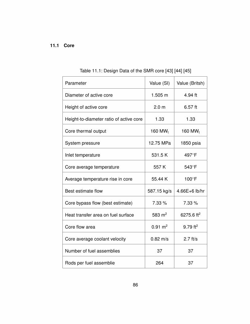
11.1 Core
Table 11.1: Design Data of the SMR core [43] [44] [45]
Parameter Value (SI) Value (Britsh)
Diameter of active core 1.505 m 4.94 ft
Height of active core 2.0 m 6.57 ft
Height-to-diameter ratio of active core 1.33 1.33
Core thermal output 160 MWt 160 MWt
System pressure 12.75 MPa 1850 psia
Inlet temperature 531.5 K 497◦F
Core average temperature 557 K 543◦F
Average temperature rise in core 55.44 K 100◦F
Best estimate flow 587.15 kg/s 4.66E+6 lb/hr
Core bypass flow (best estimate) 7.33 % 7.33 %
Heat transfer area on fuel surface 583 m2 6275.6 ft2
Core flow area 0.91 m2 9.79 ft2
Core average coolant velocity 0.82 m/s 2.7 ft/s
Number of fuel assemblies 37 37
Rods per fuel assemblie 264 37
86

Table 11.2: Design Data of Rods and Assemblies [43] [44] [45]
Parameter Value (SI) Value (Britsh)
Fuel Assemblie
Effective fuel length 243.56 cm 95.89 in
Fuel weight per assemblie 249.47 kg 550 lbm
Fuel assemblie pitch 21.5 cm 8.466 in
Fuel rod pitch 1.26 cm 0.496 in
Fuel Rod
Fuel pellet diameter 0.81 cm 0.3195 in
Fuel colum length 200 cm 78.74 in
Cladding outside diameter 0.81 cm 0.3174 in
87
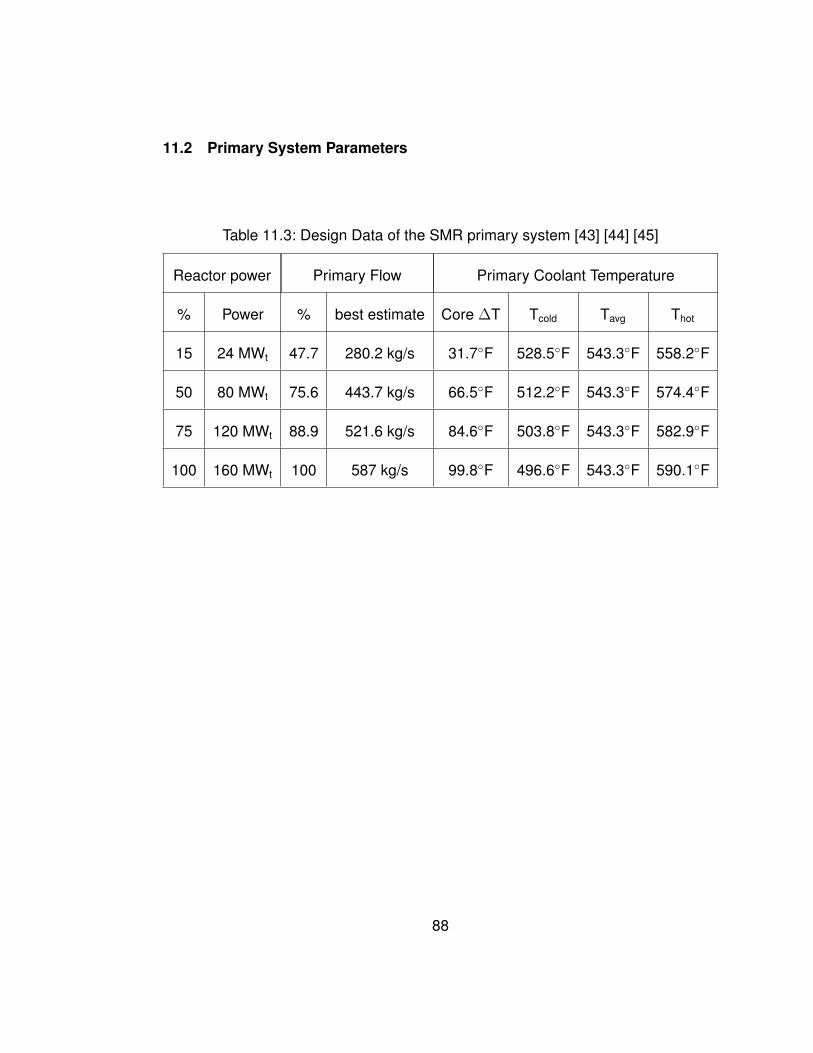
11.2 Primary System Parameters
Table 11.3: Design Data of the SMR primary system [43] [44] [45]
Reactor power Primary Flow Primary Coolant Temperature
% Power % best estimate Core ∆T Tcold Tavg Thot
15 24 MWt 47.7 280.2 kg/s 31.7◦F 528.5◦F 543.3◦F 558.2◦F
50 80 MWt 75.6 443.7 kg/s 66.5◦F 512.2◦F 543.3◦F 574.4◦F
75 120 MWt 88.9 521.6 kg/s 84.6◦F 503.8◦F 543.3◦F 582.9◦F
100 160 MWt 100 587 kg/s 99.8◦F 496.6◦F 543.3◦F 590.1◦F
88

11.3 Turbine Generator
Table 11.4: Design Data of the SMR turbine generator [43] [44] [45]
Type: Single, 10-stage condensing
Parameter Value (SI) Value (Britsh)
Operating speed 3600 1/min 3600 rpm
Phase/frequency 60 Hz 60 Hz
Estimated power 57.5 MVA 57.5 MVA
Power factor 0.85 0.85
Generator power output (electric) 50 MWe 50 MWe
Pipe diameter (sec. system) 30.48 cm 12 in
89

11.4 Primary System Geometries
Table 11.5: Geometry Data of the SMR primary system components [43] [44] [45]
Component tot. Volume Sub-Component Ave. Flow Area Length
Riser 635 ft3 Lower riser 24.9 ft2 9.4 ft
Upper riser 15.4 ft2 26.0 ft
Downcomer 1199 ft3 DC and SG 25.7 ft2 46.0 ft
Core 89 ft3 Fuel assemblies 10.3 ft2 7.9 ft
Reflector 0.9ft2 7.9 ft
Pressurizer 578 ft3 Main steam plenum 36.1 ft2 1.7 ft
Cylin. pressurizer 61.4 ft2 6.9 ft
Pressure vessel head 41.2 ft2 2.2 ft
90

Table 11.6: Volume Data of the SMR primary system components [43] [44] [45]
RCS Region Volume
Hot Leg (lower riser, riser transition, upper riser, riser supports) 635.3 ft3
Cold Leg [feedwater plenums, downcomer transition, downcomer
(lower riser), core barrel, RPV bottom head, flow diverter]
578.1 ft3
Core Region (fuel assembly region and reflector cooling chan-
nels)
88.74 ft3
SG Region 620.7 ft3
PZR Region (main steam plenums, PZR, RPV top head) 577.5 ft3
PZR Region, cylindrical (main steam plenums and PZR) 487.3 ft3
91

11.5 Steam Generator
Table 11.7: Design Data of the SMR steam generator [43] [44] [45]
Type: Helical, once-through
Parameter Value (SI) Value (Britsh)
Total heat transfer 159,13 MWt 159,13 MWt
Total number of helical tubes per NPM 1380 1380
Number of helical tube columns per NPM 21 21
Internal pressure - secondary 14.5MPa 2100 psia
External pressure - primary 14.5MPa 2100 psia
Internal temperature - secondary 616.5 K 650◦F
External temperature - primary 616.5 K 650◦F
Steam flow (full power) 67 kg/s 532100 lbm/hr
Tube wall outer diameter 15.875 mm 0.625 inches
Tube wall thickness 1.27 mm 0.050 inches
Total heat transfer area 1665.57 m2 17928 ft2
Normal steam pressure 3.45 MPa 500 psia
Normal steam temperature 574.8 K 575◦F
Design pressure upstream / downstream 14.5MPa / 6.9 MPa 2100 psia / 1000 psia
Normal feedwater temperature 422 K 300◦F
92

11.6 Development of the Model
With these geometric and thermodynamic values from the tables, it is now pos-
sible to develop a numerical model of the NuScale small modular reactor. For
the later simulation of the model, as already mentioned RELAP 5 is used. The
modeled components in RELAP 5 can be divided into three different categories
[27][28][29][30][31].
• hydrodynamic components
• heat structures
• junctions
Most of the components used in RELAP 5 are hydrodynamic components. These
simulate all parameters used in the two-fluid model and show how a reactor would
behave under certain boundary conditions. Generally, all hydrodynamic components
are simulated with a combination of single-volumes and junctions. In RELAP 5 var-
ious hydrodynamic components are preprogrammed and can be called and used
very easily. In this chapter some of these preprogrammed components will be dis-
cussed. However, only components that were used in the developed model are
discussed. The hydrodynamic components of the model used in RELAP 5 are:
• Branch
93
• Pipe
• Annulus
• Time-Dependent Volume
11.6.1 Branch
The branch component is a single volume that can be modeled with up to nine
junctions. It may be used, on the one hand, for the branching of piping systems
and, on the other hand, as an upper or lower plenum in a reactor vessel. In general,
it can be said that it is responsible for diverting and distributing a mass flow in the
system if several mass flows coincide at one point. The branch component was
used as steam generator core and upper/lower plenum in the designed model. The
input text at the end of this section shows a modeled branch component. As already
described RELAP 5 uses so-called cards to model the different components.
The first card to model a branch is the card CCC0000. The CCC stands for the
component number and can be chosen variably. The card requires two inputs. First,
the name of the component, which is also variable, and the word branch, which
defines the component type. The card CCC0001 defines the number of junctions
and the unit of the initial conditions for these junctions. To select fluid velocities,
a zero must be entered and for mass flows, a one. The next card has the number
94

CCC010N. This defines the geometrical properties, such as area length and volume,
the volume orientation and the hydrodynamic diameter of the branch. In this order,
the different values must be entered into the card. The card CCC0200 defines the
initial values for the thermodynamic properties of the fluid and also what kind of fluid
it is. The control word ebt consists of three numbers. The first two numbers define
what kind of fluid it is. To select water without boron, zero must be selected for the
first two numbers (e and b). The third number defines which initial thermodynamic
values this fluid has. To set initial values for pressure and temperature, three must
be selected as the third number (t). There are other variations for this control word
and thus it is possible that in addition to pressure and temperature other values can
be put into the card. But if t=3 only two values are expected and every other value
gives an error. Card CCC110N is about the junctions of the branch. The first value of
this card defines where a certain mass flow comes from. The second value defines
where a certain mass flow goes to. This is achieved by the value CCCXX000F. CCC
determines the component number XX the volume number and F (1 inlet, 2 outlet)
with which surface the junction is connected. The third value of this card defines the
junction area. The last card of a branch is the card CCC120N. This card specifies the
mass flows or fluid velocities of the fluid phases in junctions at the beginning of the
simulation. The values for the liquid and vapour phases are defined seperately. The
95

first value of the card establishes the initial condition of a liquid and the second value
the initial condition of vapour. The third value of this card is always zero [28][31].
RELAP 5 Branch Input
*crdno component name component type
CCC0000 "Name" branch
*crdno number of junctions vel/flw
CCC0001 X M
*crdno flowarea length volume
CCC0101 A L V
*crdno horz.orient vert.orient deltaZ
CCC0102 0.0 phi H \newline
*crdno roughness hyd. diameter fe
CCC0103 r D_h 00
*crdno vol.ic pressure temperature
CCC0200 ebt p T
*crdno from to area
CCC110N CCCXX000F CCCXX000F A_j
*crdno f.flowrate g.flowrate j.flowrate
96
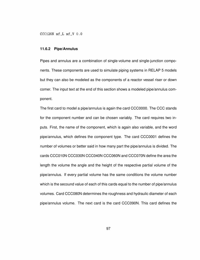
CCC120N mf_L mf_V 0.0
11.6.2 Pipe/Annulus
Pipes and annulus are a combination of single-volume and single-junction compo-
nents. These components are used to simulate piping systems in RELAP 5 models
but they can also be modeled as the components of a reactor vessel riser or down
comer. The input text at the end of this section shows a modeled pipe/annulus com-
ponent.
The first card to model a pipe/annulus is again the card CCC0000. The CCC stands
for the component number and can be chosen variably. The card requires two in-
puts. First, the name of the component, which is again also variable, and the word
pipe/annulus, which defines the component type. The card CCC0001 defines the
number of volumes or better said in how many part the pipe/annulus is divided. The
cards CCC010N CCC030N CCC040N CCC060N and CCC070N define the area the
length the volume the angle and the height of the respective partial volume of the
pipe/annulus. If every partial volume has the same conditions the volume number
which is the secound value of each of this cards equal to the number of pipe/annulus
volumes. Card CCC080N determines the roughness and hydraulic diameter of each
pipe/annulus volume. The next card is the card CCC090N. This card defines the
97

flow energy loss coefficients for forward losses (word 1) and reverse losses. (word
2). The third word of this card is the junction number and shows in which junction
the losses occur. The card CCC120N defines the initial values for pressure and
temperature and also what kind of fluid it is. Again the control word ebt consists of
three numbers. The first two numbers define what kind of fluid it is. To select water
without boron, zero must be selected for the first two numbers (e and b). The third
number defines which initial values this fluid has. To set initial values for pressure
and temperature, three must be selected as the third number (t). After the value for
the temperature there are three more values, which are not used in the model. Any
value would lead to an error. Therefore these are set to zero. The last value de-
termines the partial pipe/annulus volume. There are other variations for this control
word and thus it is possible that in addition to pressure and temperature other values
have to be put into the card. But if t=3 only two values are expected and every other
value, except zero, gives an error. The card CCC1300 determines the unit of the
initial conditions for the pipe/annulus junctions. To select fluid velocities, a zero must
be entered and for mass flows, a one. The last card of a pipe/annulus is the card
CCC130N. This card specifies the mass flows or fluid velocities of the fluid phases
in junctions at the beginning of the simulation. The values for the liquid and vapour
phases are defined seperately. The first value of the card establishes initial condition
98

of a liquid and the second value the initial condition of vapour. The third value of this
card is always zero. The last value of this card specifices the junction number. Note
the number of junctions is one less than the number of volumes [28][31].
RELAP 5 Pipe/Annulus Input
*crdno component name component type
CCC0000 "Name" pipe
*crdno number of volumes
CCC0001 N
*crdno vol.area vol.no.
CCC0101 A N
*crdno length vol.no.
CCC0301 L N
*crdno volume vol.no.
CCC0401 V N
*crdno vert.angle vol.no.
CCC0601 phi N
*crdno elev.change vol.no.
CCC0701 H N
99
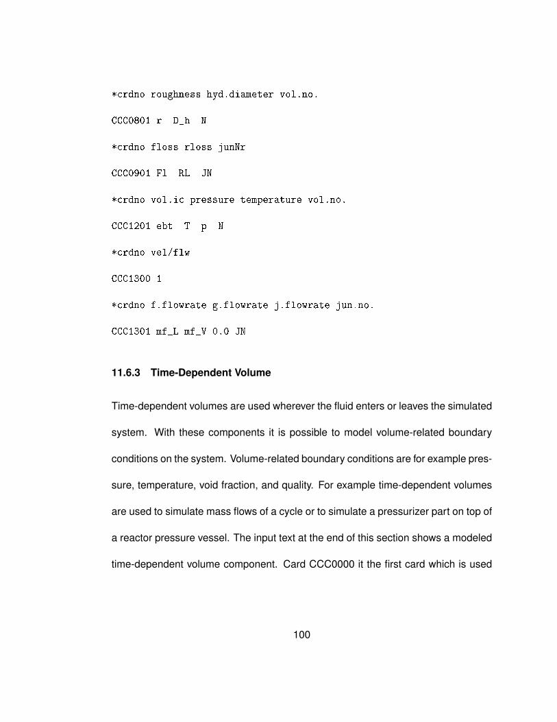
*crdno roughness hyd.diameter vol.no.
CCC0801 r D_h N
*crdno floss rloss junNr
CCC0901 Fl RL JN
*crdno vol.ic pressure temperature vol.no.
CCC1201 ebt T p N
*crdno vel/flw
CCC1300 1
*crdno f.flowrate g.flowrate j.flowrate jun.no.
CCC1301 mf_L mf_V 0.0 JN
11.6.3 Time-Dependent Volume
Time-dependent volumes are used wherever the fluid enters or leaves the simulated
system. With these components it is possible to model volume-related boundary
conditions on the system. Volume-related boundary conditions are for example pres-
sure, temperature, void fraction, and quality. For example time-dependent volumes
are used to simulate mass flows of a cycle or to simulate a pressurizer part on top of
a reactor pressure vessel. The input text at the end of this section shows a modeled
time-dependent volume component. Card CCC0000 it the first card which is used
100
to model a time-dependent volume. The CCC stands again for the component num-
ber and can be chosen variablyand the card requires two inputs. First, the name
of the component, which is again variable, and the word tmdpvol, which defines the
component type. The next card has the number CCC010N. This card defines the
geometrical properties, such as area length and volume, the volume orientation and
the hydrodynamic diameter of the time-dependent volume. In this order, the different
values must be entered into the card. The card CCC0200 defines the initial values
for the thermodynamic properties of the fluid and also what kind of fluid it is. The
control word ebt consists of three numbers. The first two numbers define what kind
of fluid it is. To select water without boron, zero must be selected for the first two
numbers (e and b). The third number defines which initial thermodynamic values
this fluid has. To set initial values for pressure and temperature, three must be se-
lected as the third number (t). There are other variations for this control word and
thus it is possible that in addition to pressure and temperature other values can be
put into the card CCC020N. But if t=3, only two values are expected and every other
value gives an error. The card CCC020N defines the thermodynamic values of the
time-dependent volume depending on a control value (tdigit). The control value can
be chosen in card CCC0200 but usually time is chosen as the value. Now for the
simulation in RELAP 5 the time-dependent volume changes its conditions depend-
101
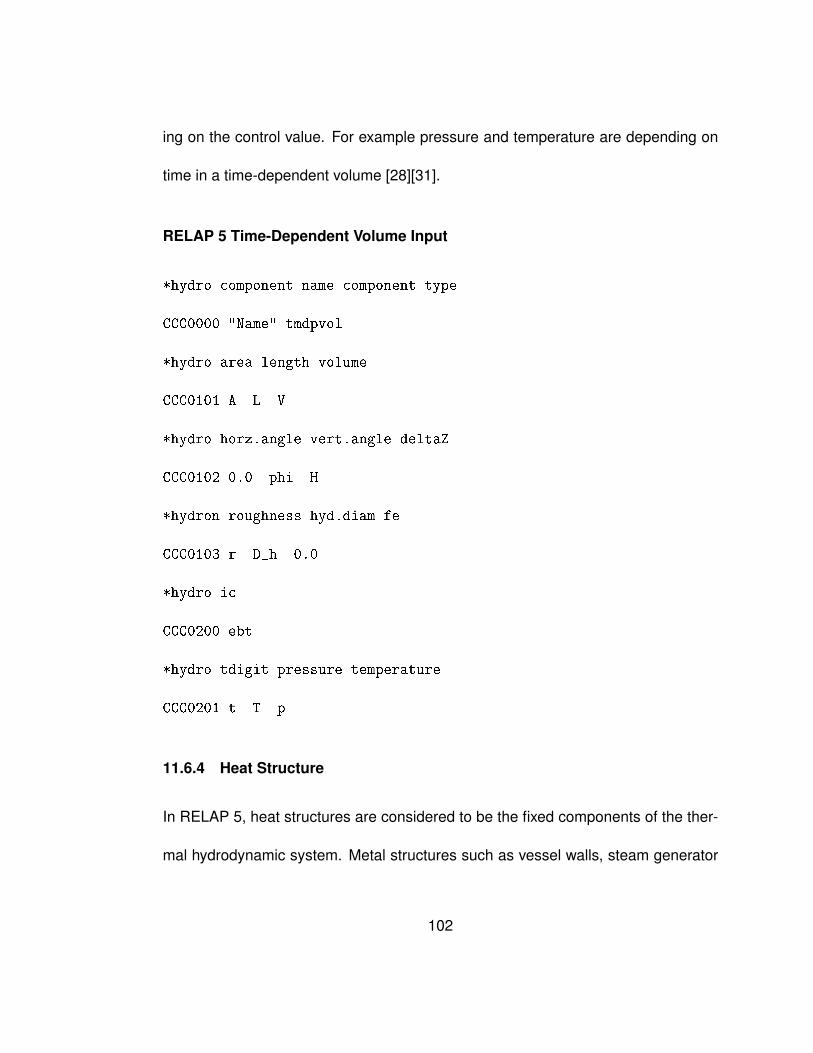
ing on the control value. For example pressure and temperature are depending on
time in a time-dependent volume [28][31].
RELAP 5 Time-Dependent Volume Input
*hydro component name component type
CCC0000 "Name" tmdpvol
*hydro area length volume
CCC0101 A L V
*hydro horz.angle vert.angle deltaZ
CCC0102 0.0 phi H
*hydron roughness hyd.diam fe
CCC0103 r D_h 0.0
*hydro ic
CCC0200 ebt
*hydro tdigit pressure temperature
CCC0201 t T p
11.6.4 Heat Structure
In RELAP 5, heat structures are considered to be the fixed components of the ther-
mal hydrodynamic system. Metal structures such as vessel walls, steam generator
102
tubes, fuel rods and reactor vessel installations are simulated with these compo-
nents. Each heat structure is simulated with a left and a right side. According to
the convention, it is only possible that each side of a heat structure is connected
to at most one hydrodynamic volume. However, it is possible that more than one
heat structure may be associated with the same hydrodynamic volume. The over-
all system response depends on the heat transferred between the heat structures
and the liquid. In addition, the temperature distributions in the heat structures are
often important simulation requirements. The input text at the end of this section
shows an example for a modeled heat structure. The first card of a heat structure
component is the card 1CCCG000. The CCC stands for the heat structure number.
This number is variable. The G stands for the geometry number which distinguishes
between different heat structures which are connected to the same volume. The
first value of this card determinates the number of axial heat structures. The second
value is the number of radial mesh points for this heat structure. The third value
inputs the geometry type of the heat structure. Enter 1 or -1 for rectangular type
, 2 or -2 for cylindrical type, or 3 or -3 for spherical type. The sign of the number
tells the program if the heat structure is coupled to its hydrodynamic component or
not. Enter a positive number for coupled and a negative number for decoupled. The
fourth value of this card is the steady-state initialization flag. Use zero if the initial
103

condition temperatures are entered on input Cards 1CCCG40N or one if the code
calculates the initial condition temperatures itself. The last value of the card is the
position of the left boundary coordinate of the heat structure. The next card is the
card 1CCCG100. This card enters the formats of the mesh point locations and how
the intervals are specified. The card 1CCCG10N specifies how many intervals there
are between the left and right boundary condition are and also which position the
right boundary condition has. In the card 1CCCG20N, the material parameters for
heat structure intervals are determinated. It is possible to simulate a heat structure
which is a combination of different layers of materials. The material values have to
be defined in tables at the end of the code. The first value of this map is the material
parameter and the second value defines how many mesh intervals are made of this
material. The card 1CCCG30N specifies the source value for every interval of the
heat structure. The next card is card 1CCCG40N. The first value of this card defines
the initial temperature of the mesh points of the heat structure and the second value
defines the mesh points. The next cards connect the heat structure to the hydrody-
namic volumes. Card 1CCCG501 is the left connection and card 1CCCG601 is the
connection to the right hydrodynamic volume of the heat structure. The first value
of these card is the connection to the volume with the word CCCXX0000. The CCC
is the component number and the XX the volume number. The next value is the
104

increment word. This value is used if the next heat structure parts are connected
to the next volumes of the hydrodynamic component. For one dimensional volumes
the increment value is 10000 or -10000 depending from which side of the hydrody-
namic component the volumes are counted. The third value defines the boundary
condition type. The fourth and fifth values are used together. If the fourth value is
zero the fifth value is the area of the left or right side of the heat structure. The last
value is the heat structure number. The card 1CCCG701 determines whether there
is a source term in the heat structure or not. The first value is the source type term.
A source term is necessary if for example a fuel rod is simulated because in the
rod heat is generated due to nuclear fission. If the heat structure simulates a steam
generator or a vessel wall no source term is necessary and the value is zero. If the
heat structure has a source, the first value is a special table which determinates how
much energy over time is generated from the heat structure. The second value of
the card is the multiplication factor for every heat structure part. If the generated en-
ergy in the whole heat structure has an heterogeneous distribution, with this value it
is possible to simulate it. The third and fourth value define which sides (left and right)
are heated by the source term. These are usually zero. The last value is the heat
structure number. The last cards of the heat structure are the cards 1CCCG800,
1CCCG900, 1CCCG801 and 1CCCG901. These cards define the boundary condi-
105

tions for the two sides of the heat structure. The cards 1CCCG800 and 1CCCG900
determine the complexity of the boundary conditions for each side of the heat struc-
ture. Both cards have a control value which defines how many boundary conditions
have to be entered in the cards 1CCCG801 and 1CCCG901. The cards of the heat
structure are 1CCCG801 and 1CCCG901. These cards determine the boundary
conditions for each side (left and right) of the heat structure [28][31].
RELAP 5 Heat Structure Input
*crdno heat.str mesh.pts geometry init.flag left.coord
1CCCG000 N MN Geo 0 left_Coor
*crdno mesh.locn.flag mesh.fmt.flag
1CCCG100 0 1
*crdno no.intervals rt.coord
1CCCG101 NoInter rt_Coor
*crdno comp.no. interval.no.
1CCCG201 Comp N.Inter
*crdno source.value mesh.int.no.
1CCCG301 S.V Mesh.Int
*crdno temperature mesh.pt.no.
106
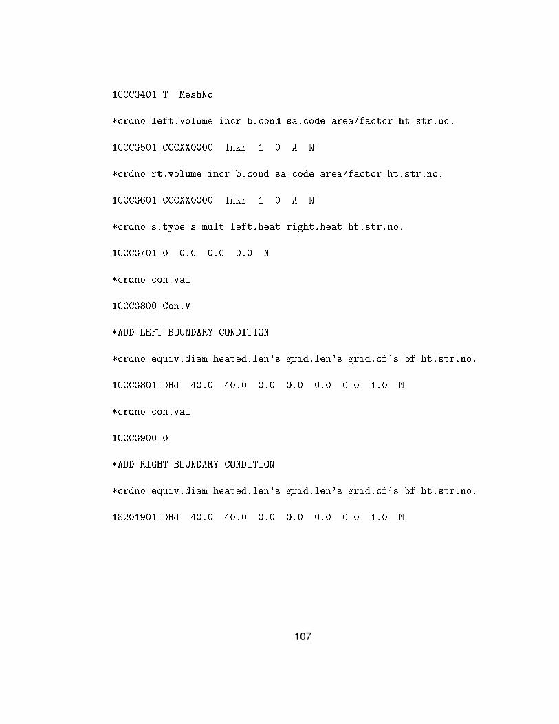
1CCCG401 T MeshNo
*crdno left.volume incr b.cond sa.code area/factor ht.str.no.
1CCCG501 CCCXX0000 Inkr 1 0 A N
*crdno rt.volume incr b.cond sa.code area/factor ht.str.no.
1CCCG601 CCCXX0000 Inkr 1 0 A N
*crdno s.type s.mult left.heat right.heat ht.str.no.
1CCCG701 0 0.0 0.0 0.0 N
*crdno con.val
1CCCG800 Con.V
*ADD LEFT BOUNDARY CONDITION
*crdno equiv.diam heated.len's grid.len's grid.cf's bf ht.str.no.
1CCCG801 DHd 40.0 40.0 0.0 0.0 0.0 0.0 1.0 N
*crdno con.val
1CCCG900 0
*ADD RIGHT BOUNDARY CONDITION
*crdno equiv.diam heated.len's grid.len's grid.cf's bf ht.str.no.
18201901 DHd 40.0 40.0 0.0 0.0 0.0 0.0 1.0 N
107

11.6.5 Single-Junction
The single-junction component is used to connect other components, for example
pipe or time-dependent volumes, to each other. Initial junction conditions of this
component are fluid velocities or mass flow rates. The input text at the end of this
section shows a modeled single-junction. Card CCC0000 is the first card which is
used to model a single-junction. The CCC stands again for the junction number and
can be chosen variably. The card requires two inputs. The first junction input is
the name of the junction, which is like the component names variable, and the word
sngljun, which defines the junction type. The card CCC0101 is about the connected
components. The first value of this card defines from which component the certain
mass flow comes from. The second value defines to which component the certain
mass flow goes to. This is achieved by the value CCCXX000F. CCC determines
the component number XX the volume number and F (1 inlet, 2 outlet) with which
surface the junction is connected. The third value of this card defines the area of
the junction. The card CCC0201 determines the unit of the initial conditions for the
single-junction and specifies the mass flows or fluid velocities of the fluid phases in
single-junction at the beginning of the simulation. To select fluid velocities the first
value of this card has to be a zero. To select mass flows a one has to be entered.
The values for the liquid and vapour phases are defined seperately. The second
108

value of the card establishes initial condition of a liquid and the third value the initial
condition of vapour. The fourth value of this card is always zero [28][31].
RELAP 5 Single-Junction Input
*hydro component name component type
CCC0000 "Name" sngljun
*hydro from to area f.loss r.loss fvcahs
CCC0101 CCCXX000F CCCXX000F A_j 0.0 0.0 0
*hydro f.flowrate g.flowrate j.flowrate
CCC0201 1 mf_L mf_Vb 0.0
11.6.6 Time-Dependent Junction
Time-dependent junction components are used when fluid velocities or mass flow
rates are a function of time or another time-advanced quantity. With these com-
ponents it is possible to model flow boundary conditions on the simulated system.
The boundary conditions can be specified as either a volumetric or mass flow rate.
Time-dependent junctions can connect like single-junctions, two different system
volumes or time-dependent volumes. The input text at the end of this section shows
a modeled time-dependent junction. The first card of a time-dependent junction
component is the card CCC0000. Again the CCC stands for the junction number
109

and can be chosen variably. The card requires two inputs. The first junction input is
the name of the junction, which is also variable, and the word tmdpjun, which defines
the junction type. The card CCC0101 is about the connected components. The first
value of this card defines from which component the certain mass flow comes from.
The second value defines to which component the certain mass flow goes to. This is
achieved by the value CCCXX000F. CCC determines the component number XX the
volume number and F (1 inlet, 2 outlet) with which surface the junction is connected.
The third value of this card defines the area of the junction. The first value of card
CCC0200 determines the unit of the initial conditions for the time-dependent junc-
tions. A zero must be entered to select fluid velocities and a one for mass flows. The
three other values are optional trip and control values. The card CCC020N defines
the fluid velocity or mass flow rate of the different phases of the fluid depending on
a control value (tdigit). For example the mass flow rate is changed over time. The
control value can be chosen in card CCC0200 but usually time is chosen as the
value. Now for the simulation in RELAP 5, the time-dependent junction changes its
conditions depending on the control value [28][31].
RELAP 5 Time-Dependent Junction Input
*hydro component name component type
110

CCC0000 "Name" tmdpjun
*hydro from to area
CCC0101 CCCXX000F CCCXX000F A_j
*hydro vel/flw trip.no.
CCC0200 1
*hydro tdigit f.flowrate g.flowrate j.flowrate
CCC020N t mf_L mf_V 0.0
11.6.7 Valve Junction
In general valve junction components have the capability to vary the flow area. Each
valve type has its own input rules, which will not be discussed here. Eight valves out
of six types can be chosen in RELAP 5. The types are:
• check valves (CHKVLV)
• trip valves (TRPVLV)
• inertial swing check valves (TRPVLV)
• motor valves (MTRVLV)
• servo valves (SRVVLV)
• relief valves (RLFVLV)
111
The input text at the end of this section shows an example for a modeled trip valve.
The first card of a valve junction component is the card CCC0000. The CCC stands
again for the junction number and can be chosen variably. The card requires two
inputs. The first junction input is the name of the junction, which is also variable, and
the word valve, which defines the junction type. The card CCC0101 deals with the
connected components. The first value of this card defines from which component
the certain mass flow comes from. The second value defines to which component
the certain mass flow goes to. This is achieved by the value CCCXX000F. CCC
determines the component number XX the volume number and F (1 inlet, 2 outlet)
with which surface the junction is connected. The third value of this card defines the
area of the junction. The next card has the number CCC0200. The first value of
this card determines the unit of the initial conditions for the valve junction. To select
fluid velocities, a zero must be entered and for mass flow rates, a one. The next
values specify the mass flow rates or fluid velocities of the fluid phases in junctions
at the beginning of the simulation. The values for the liquid and vapour phases are
defined seperately. The second value of the card establishes the initial condition of
the liquid and the third value the initial condition of the vapour. The fourth value of
this card is always zero. With the card CCC0300, the valve type is determinted. In
this example, a trip valve was chosen thus enter the control word trpvlv. The other
112

control words can be found in the list at the beginning of the section. The input of
the next card CCC0301, is dependent on the type of valve which was chosen. In
this case the values for a trip valve have to be entered. For trip valves only the trip
number is necessary. This value makes a link to the trip which controls the valve
[28][31].
RELAP 5 Valve Junction Input
*crdno Name Type
CCC0000 "Name" valve
*hydro from to area
CCC0101 CCCXX000F CCCXX000F A_v
*crdno vel/flw f.flowrate g.flowrate j.flowrate
CCC0201 1 mf_L mf_V 0.0
*crdno Valvetype
CCC0300 trpvlv
*crdno TripNumber
CCC0301 trip
113

11.7 The Model
The next step was to summarize the information in the tables as well as the informa-
tion about the various RELAP 5 components in a thermal hydraulic model. The input
of the model can be seen in Appendix 16. The next two figures show a schematic
representation and the nodalization diagram of the simulated NuScale reactor. The
numbering in the figures is the same in the model in the appendix.
114

Figure 11.1: Schematic representation of the SMR RELAP 5 Model.
115

Figure 11.2: Nodalization diagram of a SMR RELAP 5 Model.
116

12 Steady State Model
The next step in the development of the SMR model is to reach steady state cond-
tions. This means the calculated values of the model do not change over time. To
reach these conditions, RELAP 5 has to run the model for a long time. The time to
reach steady state was 5000 seconds. The most important calculated values are
pressure, temperature, void fraction, and mass flow at the different volumes and
junctions of the SMR model. Especially the parameter at the inlet and outlet of the
core and the steam generator primary and secondary are very important. At the
heat structures of the core, heat is generated. This heat is then transported by the
liquid water to the steam generator in the primary loop. The heat structures of the
steam generator transfer the heat to the secondary side which is in steady state from
the beginning of the simuation, because it is an open cycle. The simulated reactor
has a thermal power of 160 MW. Therefore the fuel rods have to produce 160 MW
and the heat structures of the steam generator have to move this amount of power
from the primary side to the secondary side. The heat transfer can be calculated by
117

the following equation.
Qth = m · (hout − hin) (12.1)
The enthalpies in this eqaution depend on the temperature and the pressure of the
fluid in the volume. With the help of thermodynamic steam tables, it is possible
to interpolate the enthalpy for the calculated parameters. The next figure shows a
shematic of the reactor model and where the different components are located. This
shematic figure will help the reader to better understand what processes occur in
the simulated model.
118

Figure 12.1: Schematic representation of the model.
119

Table 12.1: Model Component Data
Component number Name Type Volumes
100 Lower Plenum Branch 1
110 Core Pipe 8
120 Core Pipe 8
200 Lower Riser Pipe 7
210 Middle Riser Pipe 5
220 Upper Riser Pipe 25
350 Upper Plenum Branch 1
360 Pressurizer Branch 1
400 Steam Generator Pipe 15
401 Steam Generator Pipe 15
500 Down comer Pipe 20
501 Down comer Pipe 20
740 Source Tim.Dep.Volume 1
760 Feed Water Pipe Pipe 25
790 Steam Pipe Pipe 25
800 Sink Tim.Dep.Volume 1
1801 Fuel Rods Heat Structure 8
1802 SG-Tubes Heat Structure 15120

The next sections show the measured values at the specific volumes over the
simulation time.
12.1 Core
The core in the model is located between component 100 (lower plenum) and com-
ponent 200 cell 1 (lower riser). At these specific volumes the measurements are
made. The next figures show the pressure and temperature over time in both vol-
umes.
121
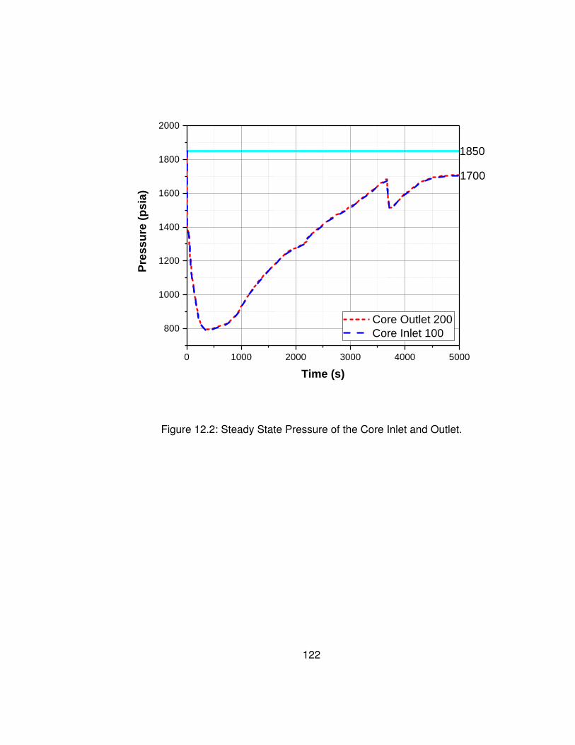
0 1 0 0 0 2 0 0 0 3 0 0 0 4 0 0 0 5 0 0 0
8 0 0
1 0 0 0
1 2 0 0
1 4 0 0
1 6 0 0
1 8 0 0
2 0 0 0
1 7 0 0
Pres
sure
(psia)
T i m e ( s )
C o r e O u t l e t 2 0 0 C o r e I n l e t 1 0 0
1 8 5 0
Figure 12.2: Steady State Pressure of the Core Inlet and Outlet.
122

0 1 0 0 0 2 0 0 0 3 0 0 0 4 0 0 0 5 0 0 0
4 8 0
5 0 0
5 2 0
5 4 0
5 6 0
5 8 0
6 0 0
5 2 8
Liquid
Temp
eratur
e (F)
T i m e ( s )
C o r e I n l e t 1 0 0 C o r e O u t l e t 2 0 0
5 0 0
5 9 0
Figure 12.3: Steady State Temperature of the Core Inlet and Outlet.
At the beginning of the simulation it is clearly seen that RELAP 5 calculates to
reach steady state conditions. After 4500 seconds, pressure and temperaure are
constant. At this point the model is in steady state. The steady state pressure and
the steady state temperatures have the values of 1700 psi, 590◦F and 528◦F. Figure
12.2, it is seen that the pressures from the core inlet and core outlet are slightly
123

different. The reason for this is hydrostatics because the inlet is lower than the outlet.
But the difference is very small and thus it can be neglected. The pressure is a little
bit lower than expected but the difference is only 150 psi. The biggest problem with a
lower pressure is the corresponding lower boiling temperature. But in this simulation
this is not a problem because the boiling temperature for a pressure of 1850 psi is
624.9◦F and for 1700 psi 613.9◦F. This is a small difference and can be neglected
due to the fact that the highest temperature in the simulation is approximatly 25◦F
away from this point. The temperature difference is approximatly 62◦F compared to
expected 90◦F. This can be explained by the frictional losses in the system. Frictional
losses in the primary loop are very important in determining the actual pressure drop
and therefore, mass flow rate, heat transfer, pressures, and temperatures. In the
simulation all components are simulated as smooth, thus fictional losses are small.
Only in the core and steam generator components are values implemented which
slow down the circulation. The result of this lower temperature difference is a higher
mass flow rate in the system to compensate for this condition. When RELAP 5 has
reached steady state conditions, it is possible to show how much energy the core has
input into the system. For this purpose, thermodynamic steam tables can be used to
calculate the enthalpy of the fluid inside the system before entering and after leaving
the core. The entalpy values are houtC = 1398.9 kJ/kg and hinC = 1211.4 kJ/kg. To
124

calcutale the power of the core it is necessary to look up the steady state mass flow
rate of the core. RELAP 5 measures mass flow rates in the junctions and not in the
volumes of its models. To see the right mass flow rates, the junctions of the core
inlet and core outlet have to be checked. Because the core in this model is divided
into two parts, both mass flows have to be added into one single mass flow to show
the total mass flow rate in the core components. The mass flow rates can be seen
in the next figure.
125

0 1 0 0 0 2 0 0 0 3 0 0 0 4 0 0 0 5 0 0 0
6 0 0
8 0 0
1 0 0 0
1 2 0 0
1 4 0 0
9 3 1
Liquid
Mas
sflow
lbm/
s
T i m e ( s )
C o r e 3 0 0 & 3 0 1
6 4 7
Figure 12.4: Steady State Massflow in the Core.
The next figure shows the densities in the core inlet and core outllet. The density
difference is the driving force in natural circulation and leads to the movement of
the liquid water in the simulated SMR reactor. It is clearly seen in figure 12.5 that a
density difference occurs between core inlet and core outlet. In addition to that it is
seen in figure 12.4 that mass moves through the system. This result is the proof for
126

the existence of natural circulation in the simulated SMR reactor.
0 1 0 0 0 2 0 0 0 3 0 0 0 4 0 0 0 5 0 0 0
4 3
4 4
4 5
4 6
4 7
4 8
4 9
5 0De
nsity
(lbm
/ ft3)
T i m e ( s )
C o r e I n l e t 1 0 0 C o r e O u t l e t 2 0 0
Figure 12.5: Steady State Density at the Core Inlet and Outlet.
It is seen at the beginning of the simulation that the steady state mass flow rates
in figure 12.4 has to be reached like the pressure and temperatures. After this time,
the mass flow rates are constant and have a value of 931 lbm/s. Again this is a little
bit higher because of the lower temperature difference. The primary loop is liquid
127

water only because of the relativly high pressure of the system. That is shown by the
calculation of the enthalpies and in the next figure which shows the liquid fraction of
the appropriate volumes.
0 1 0 0 0 2 0 0 0 3 0 0 0 4 0 0 0 5 0 0 00 , 0
0 , 2
0 , 4
0 , 6
0 , 8
1 , 0
Liquid
Frac
tion (
-)
T i m e ( s )
C o r e I n l e t 1 0 0 C o r e O u t l e t 2 0 0 P r e s s u r i z e r 3 6 0
Figure 12.6: Steady State Liquid Fraction at the Core Inlet and Outlet.
With the steady state volumes for enthalpy and mass flow it is now possible to
calculate the power of the core. The power can be calculated with equation 12.1.
128
The result is 158.69 MW. This shows the model works and the correct power level is
reached.
12.2 Steam Generator Primary
The primary steam generator in the model is located between component 350 (upper
plenum), component 500 (down comer) and component 501 (down comer). For all
components the first cell is used. At these specific volumes the measurements are
made. It is necessary to check temperatures, pressures and mass flow rates at the
inlet and outlet of the steam generator. The next figures show the pressure and
temperature over time in the measured volumes.
129

0 1 0 0 0 2 0 0 0 3 0 0 0 4 0 0 0 5 0 0 06 0 0
8 0 0
1 0 0 0
1 2 0 0
1 4 0 0
1 6 0 0
1 8 0 0
2 0 0 0
1 7 0 0
Pres
sure
(psia)
T i m e ( s )
S G I n l e t 4 0 0 C e l l 1 S G O u t l e t 4 0 1 C e l l 1 5
1 8 5 0
Figure 12.7: Steady State Pressure at the Steam Generator Inlet and Outlet.
130

0 1 0 0 0 2 0 0 0 3 0 0 0 4 0 0 0 5 0 0 0
4 8 0
5 0 0
5 2 0
5 4 0
5 6 0
5 8 0
6 0 0
5 2 8
D o w n C o m e r 5 0 0 & 5 0 1 U p p e r P l e m u m 3 5 0
Liquid
Temp
eratur
e (F)
T i m e ( s )
5 9 0
5 0 0
Figure 12.8: Steady State Temperature at the Steam Generator Inlet and Outlet.
Again it is clearly seen that RELAP 5 at the beginning of the simulation tries to
reach steady state. After 4500 seconds the steady state temperatures are TH=590◦F
and TC=528◦F and the steady state pressure is 1700 psi. The steam generator is
located between the hot leg and the cold leg of the reactor high pressure cycle. It
has the function to remove all the heat energy which is produced in the core to the
131

secondary side. As already calculated the power of the core is 158.69 MW. The
same power has to be removed by the steam generator. The reasons that the pa-
rameters are not exactly the parameters from the tables from the previous chapter
are the same as already described in the previous subchapter. With these parame-
ters for pressure and temperature, it is again possbile to look up the enthalpies for
the hot leg and the cold leg of the reactor. From the steam tables, the enthalpies
are hH=1398.9 kJ/kg and hC=1211.4 kJ/kg. To calculate the removed heat in the
steam generator the mass flow rate is needed. The next figure shows the mass flow
through the primary side of the steam generator.
132
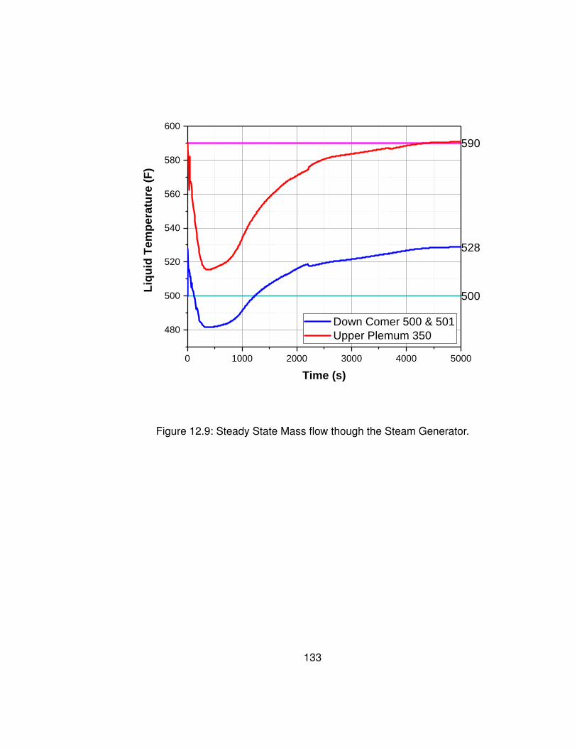
0 1 0 0 0 2 0 0 0 3 0 0 0 4 0 0 0 5 0 0 0
4 8 0
5 0 0
5 2 0
5 4 0
5 6 0
5 8 0
6 0 0
5 2 8
D o w n C o m e r 5 0 0 & 5 0 1 U p p e r P l e m u m 3 5 0
Liquid
Temp
eratur
e (F)
T i m e ( s )
5 9 0
5 0 0
Figure 12.9: Steady State Mass flow though the Steam Generator.
133
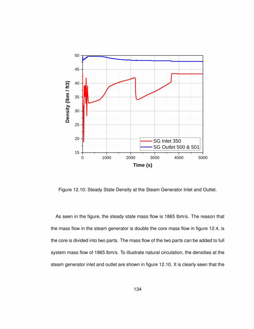
0 1 0 0 0 2 0 0 0 3 0 0 0 4 0 0 0 5 0 0 01 5
2 0
2 5
3 0
3 5
4 0
4 5
5 0
Dens
ity (lb
m / ft
3)
T i m e ( s )
S G I n l e t 3 5 0 S G O u t l e t 5 0 0 & 5 0 1
Figure 12.10: Steady State Density at the Steam Generator Inlet and Outlet.
As seen in the figure, the steady state mass flow is 1865 lbm/s. The reason that
the mass flow in the steam generator is double the core mass flow in figure 12.4, is
the core is divided into two parts. The mass flow of the two parts can be added to full
system mass flow of 1865 lbm/s. To illustrate natural circulation, the densities at the
steam generator inlet and outlet are shown in figure 12.10. It is clearly seen that the
134
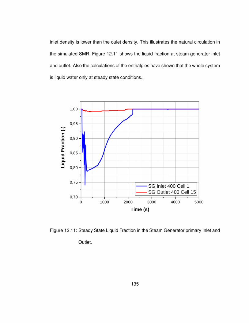
inlet density is lower than the oulet density. This illustrates the natural circulation in
the simulated SMR. Figure 12.11 shows the liquid fraction at steam generator inlet
and outlet. Also the calculations of the enthalpies have shown that the whole system
is liquid water only at steady state conditions..
0 1 0 0 0 2 0 0 0 3 0 0 0 4 0 0 0 5 0 0 00 , 7 0
0 , 7 5
0 , 8 0
0 , 8 5
0 , 9 0
0 , 9 5
1 , 0 0
Liquid
Frac
tion (
-)
T i m e ( s )
S G I n l e t 4 0 0 C e l l 1 S G O u t l e t 4 0 0 C e l l 1 5
Figure 12.11: Steady State Liquid Fraction in the Steam Generator primary Inlet and
Outlet.
135

Figure 12.11 shows that at the beginning of the simulation, boiling happens in the
steam generator. This is because of the pressure drop at the beginning of the simu-
lation which is seen in figure 12.7. This pressure drop is caused by the inconsistency
of the choosen initial conditions of the simulation model. The removed heat can be
calculated with equation 12.1. The results is 158.69 MW. This result is the same as
in the produced power in the core. Therefore the reactor has reached steady state.
12.3 Steam Generator Secondary
The steam generator secondary in the model is located between component 760
(Watpip) cell 25 and component 790 (Stepi) cell 1. In the steam generator secondary
side, the fluid makes a phase change from liquid to vapor. In cell 25 of component
760 (inlet), the fluid state is liquid and in cell 1, of component 790 (outlet) the fluid
state is vapor. The following figures show the liquid and vapor fractions at the inlet
and outlet of the secondary steam generator.
136

0 1 0 0 0 2 0 0 0 3 0 0 0 4 0 0 0 5 0 0 0
0 , 0
0 , 2
0 , 4
0 , 6
0 , 8
1 , 0Liq
uid Fr
actio
n (-)
T i m e ( s )
S e c . S G I n l e t S e c . S G O u t l e t
Figure 12.12: Liquid Fraction of the Steam Generator sec. side Inlet and Outlet.
137

0 1 0 0 0 2 0 0 0 3 0 0 0 4 0 0 0 5 0 0 0
0 , 0
0 , 2
0 , 4
0 , 6
0 , 8
1 , 0Vo
id Fra
ction
(-)
T i m e ( s )
S e c . S G I n l e t S e c . S G O u t l e t
Figure 12.13: Vapor Fraction at the Steam Generator sec. side Inlet and Outlet.
As clearly seen in the two figures, the fluid before the steam generator is solid
liquid and after leaving it the fluid is fully vapor. Therefore, it is verified that the
entering liquid makes a phase change to vapor inside the steam generator. The
next figure shows boiling development in the steam generator cells over time.
138

0 1 0 0 0 2 0 0 0 3 0 0 0 4 0 0 0 5 0 0 00 , 0
0 , 2
0 , 4
0 , 6
0 , 8
1 , 0Vo
id Fra
ction
Liqu
id (-)
T i m e ( s )
S e c . S G C e l l 1 S e c . S G C e l l 3 S e c . S G C e l l 4 S e c . S G C e l l 5 S e c . S G C e l l 1 3
Figure 12.14: Liquid Fraction in the Steam Generator sec. Cells.
It is seen in figure 12.14 that the fluid state in the first cell of the secondary steam
generator is solid liquid. At the third cell the fluid changed about 50 percent from
liquid to vapor. It is also seen that the rate of conversion drops over time. While at
the beginning (cell 1 to cell 3) 50 percent of the liquid made a phase change, only
10 percent of the liquid made a phase change at the end of the steam generator
139

(cell 5 to cell 13). The reason for this is that some of the heat energy is taken to
superheat the steam and is not used to phase change the rest of the liquid. To see
what condtions the fluid has before entering and after exiting the steam generator it
is necassary to look up the liquid and vapor temperatures for component 760 and
790. Because RELAP 5 expects to have liquid and vapor in every volume, it always
calculates the temperatures for both fractions in every volume. The next figures
show the temperatures of the fluid.
140
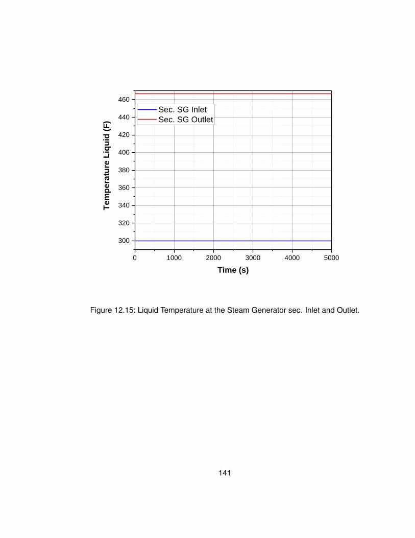
0 1 0 0 0 2 0 0 0 3 0 0 0 4 0 0 0 5 0 0 03 0 0
3 2 0
3 4 0
3 6 0
3 8 0
4 0 0
4 2 0
4 4 0
4 6 0Te
mpera
ture L
iquid
(F)
T i m e ( s )
S e c . S G I n l e t S e c . S G O u t l e t
Figure 12.15: Liquid Temperature at the Steam Generator sec. Inlet and Outlet.
141

0 1 0 0 0 2 0 0 0 3 0 0 0 4 0 0 0 5 0 0 04 6 0
4 8 0
5 0 0
5 2 0
5 4 0
5 6 0
5 8 0
6 0 0Te
mpera
ture V
apou
r (F)
T i m e ( s )
S e c . S G I n l e t S e c . S G O u t l e t
Figure 12.16: Vapor Temperature at the Steam Generator sec. Inlet and Outlet.
It is seen in the figures that the liquid before entering the steam generator has a
temperature of 300◦F specified by fixed boundary conditions. The vapor after leaving
the steam generator has a temperature of 565◦F. With the help of steam tables, it is
observed that the outlet vapor has superheated conditions and the inlet liquid has
subcooled conditions. It is also possible to look up the enthalpies for the liquid and
142

vapor. The liquid inlet enthalpy is hin=629.34 kJ/kg and the vapor outlet enthalpy is
hout=2970.4 kJ/kg. The pressure is the second variable to calculate the enthalpies
and thus the conditions of the fluid. The next figures show the pressures of the inlet
and outlet of the secondary steam generator.
0 1 0 0 0 2 0 0 0 3 0 0 0 4 0 0 0 5 0 0 0
4 9 5
5 0 0
5 0 5
5 1 0
5 1 5
Pres
sure
(psia)
T i m e ( s )
S e c . S G I n l e t S e c . S G O u t l e t
Figure 12.17: Pressure of the Steam Generator sec. Inlet and Outlet.
The mass flow rate of the two phase fluid though the secoandary steam generator
143
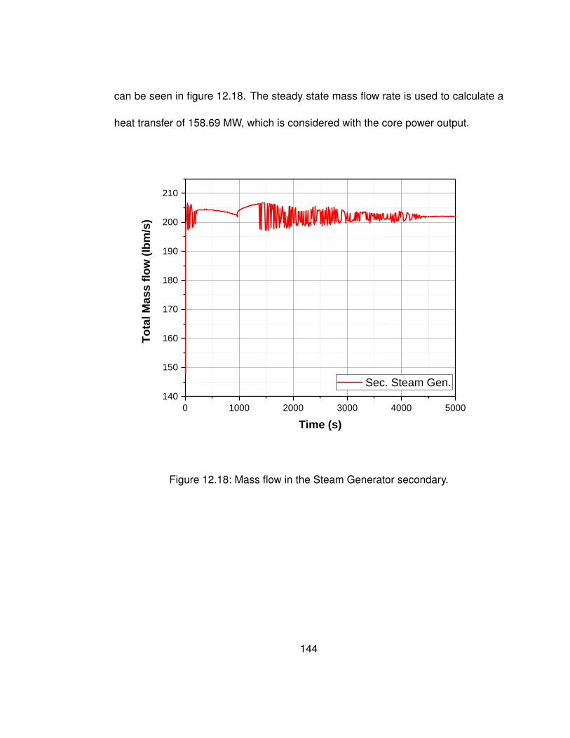
can be seen in figure 12.18. The steady state mass flow rate is used to calculate a
heat transfer of 158.69 MW, which is considered with the core power output.
0 1 0 0 0 2 0 0 0 3 0 0 0 4 0 0 0 5 0 0 01 4 0
1 5 0
1 6 0
1 7 0
1 8 0
1 9 0
2 0 0
2 1 0
Total
Mas
s flow
(lbm/
s)
T i m e ( s )
S e c . S t e a m G e n .
Figure 12.18: Mass flow in the Steam Generator secondary.
144
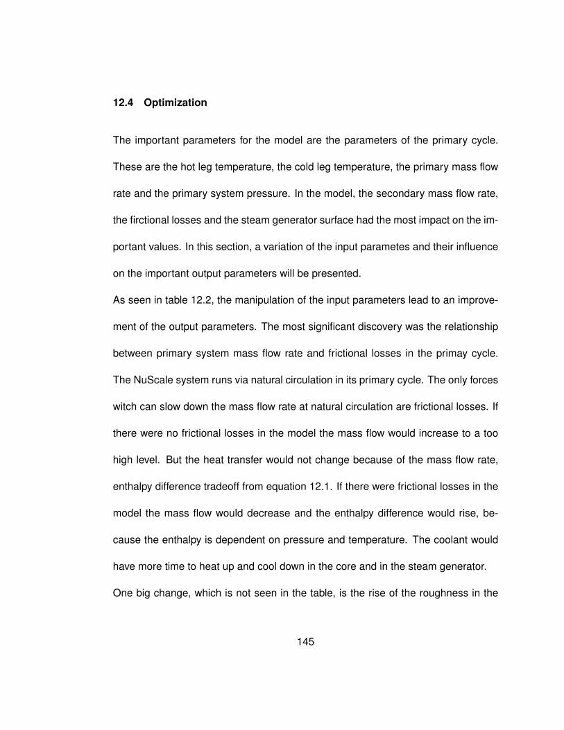
12.4 Optimization
The important parameters for the model are the parameters of the primary cycle.
These are the hot leg temperature, the cold leg temperature, the primary mass flow
rate and the primary system pressure. In the model, the secondary mass flow rate,
the firctional losses and the steam generator surface had the most impact on the im-
portant values. In this section, a variation of the input parametes and their influence
on the important output parameters will be presented.
As seen in table 12.2, the manipulation of the input parameters lead to an improve-
ment of the output parameters. The most significant discovery was the relationship
between primary system mass flow rate and frictional losses in the primay cycle.
The NuScale system runs via natural circulation in its primary cycle. The only forces
witch can slow down the mass flow rate at natural circulation are frictional losses. If
there were no frictional losses in the model the mass flow would increase to a too
high level. But the heat transfer would not change because of the mass flow rate,
enthalpy difference tradeoff from equation 12.1. If there were frictional losses in the
model the mass flow would decrease and the enthalpy difference would rise, be-
cause the enthalpy is dependent on pressure and temperature. The coolant would
have more time to heat up and cool down in the core and in the steam generator.
One big change, which is not seen in the table, is the rise of the roughness in the
145

riser and in the downcomer of the model. This can be seen in the appendix where
the input model is located. The calculated pressure and the hot leg temperature at
the last case are exactly the same as in the final safety analysis report of NuScale.
The calculated cold leg temperature and the primary mass flow rate are still higher
than expected, especially the mass flow rate is higher than in the final safety analy-
sis report of NuScale.
In addtion to that, it is possible to look up the enthalpies in the thermodynamic steam
tables for the exact pressure and temperatures from the NuScale FSAR. Together
with the exact mass flow rate from the FSAR, it is possible to calculate the trans-
ferred heat in the system. This value is only approximatly 154 MW, expacted was
160 MW. This is a reason why the mass flow rate in the developed model is higher
than expected. In RELAP 5 there are plenty of optional cards which could be used
to reach the final and expected steady state of the system, but this would be too
complicated for this simple model and for this reason the eighth case is the final
steady state of the model for the futher development of the model.
146
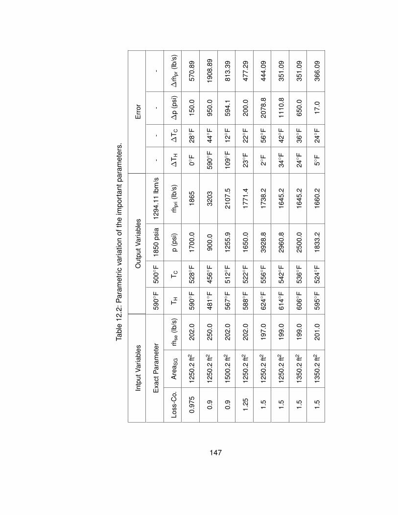
Tabl
e12
.2:P
aram
etric
varia
tion
ofth
eim
port
antp
aram
eter
s.
Intp
utVa
riabl
esO
utpu
tVar
iabl
esE
rror
Exa
ctP
aram
eter
590◦
F50
0◦F
1850
psia
1294
.11
lbm
/s-
--
-
Loss
-Co.
Are
a SG
mse
(lb/s
)T H
T Cp
(psi
)m
pri(lb
/s)
∆T H
∆T C
∆p
(psi
)∆
mpr
(lb/s
)
0.97
512
50.2
ft220
2.0
590◦
F52
8◦F
1700
.018
650◦
F28◦ F
150.
057
0.89
0.9
1250
.2ft2
250.
048
1◦F
456◦
F90
0.0
3203
590◦
F44◦ F
950.
019
08.8
9
0.9
1500
.2ft2
202.
056
7◦F
512◦
F12
55.9
2107
.510
9◦F
12◦ F
594.
181
3.39
1.25
1250
.2ft2
202.
058
8◦F
522◦
F16
50.0
1771
.423◦ F
22◦ F
200.
047
7.29
1.5
1250
.2ft2
197.
062
4◦F
556◦
F39
28.8
1738
.22◦
F56◦ F
2078
.844
4.09
1.5
1250
.2ft2
199.
061
4◦F
542◦
F29
60.8
1645
.234◦ F
42◦ F
1110
.835
1.09
1.5
1350
.2ft2
199.
060
6◦F
536◦
F25
00.0
1645
.224◦ F
36◦ F
650.
035
1.09
1.5
1350
.2ft2
201.
059
5◦F
524◦
F18
33.2
1660
.25◦
F24◦ F
17.0
366.
09
147

13 Further Development
The RELAP 5 model of the NuScale small modular reactor presented in this thesis
has much potential. At the moment only a closed primary loop and an open sec-
ondary loop is modeled and tested. The NuScale SMR reactor has two passive
safety systems which are called emergency core cooling system (ECCS) and decay
heat removal system (DHRS). The ECCS and DHRS system were discussed in the
previous chapters. These two systems can be added to the NuScale model in the
future. Figure 13.1 shows schematic the enhanced model. The differences can be
cleary seen in this figure when compared to Figure 12.1. To model these passive
safety systems, pipes, junctions, and valves would be used in RELAP 5. After the
development of the new model, it is possible to test and evaluate several accident
scenarios with the new modeled passive safety systems. Examples for accident
scenarios are:
• Steam generator tube rupture
• Failure of secondary cooland pump
148

• Accidental opening of a vent valve
• Small break in the primary system
149

Figure 13.1: Schematic representation of the future SMR model.
150

14 Conclusions
The goal of this research was to develop a thermal hydraulic model to simulate the
NuScale design small modular reactor with RELAP 5. The first step for this work
was to survey design of small modular reactors (SMRs) and technology aspects.
Furthermore, since the simulated NuScale SMR is an integral PWR, the operation
of pressurized water reactors needed to be exammed to develop the model. The
NuScale design as descibed in the final safety analysis report formed the basis of
this model. A detailed of the NuScale small modular reactor was developed for
achieving a steady state. The model has two main parts, a closed primary cycle
and an open secondary cycle. It was achieved to model all components of the
NuScale SMR and run a simulation where the steady state parameters of the FSAR
and the calculated RELAP 5 parameters apporximatly matched. The significance
of this verification was that it was proven that this reactor design works, also when
it is only viewed from a physical-mathematical point. The steady state is the basis
for all other following accident simulations. In the steady state simulation, it could
151

be verified that the NuScale SMR design as described in the final safety analysis
report is consistent. However, it was also discvered that frictional losses play a
significant role in the NuScale system balance of mass flow and heat transfer. Also,
it was shown that natural circulation only is enough to operate this kind of reactor.
These basis simulations showed the great potencial of the NuScale design and the
corresponding developed RELAP 5 model. For future work it will be necessary to
improve the RELAP 5 model and program more parts of the whole NuScale SMR
system. An example could be the two passive safety systems, DHRS and ECCS.
The addition of these system would give the model a greater complexity and would
improve the scope of application. At the end the model could be used to predict
and analyse several operation and accident scenarios, which is significant because
it would be not necessary anymore to wait for experimental data from hardware
reactor models. This would lead to a fast development and would safe time and
money. This work will be part of further development of the RELAP 5 Nuscale SMR
model.
152

15 Appendix Nomenclature
15.1 Latin letters
t time (s)
x spatial variable (m)
υ fluid velocity ( ms-1 )
υi interphase velocity ( ms-1 )
A cross-sectional area (m2)
V volume(m3)
m mass (Kg)
W mass flow (Kgs-1)
P pressure (Pa)
Bx projection of gravity onto the pipe direction (ms-2)
153

FW wall friction coefficient (s-1)
FI interphase friction coefficient (s-1)
C virtual mass coefficient (non-dimensional) compressibility (m3)
K local pressure drop coefficient (non-dimensional)
HLOSS form loss coefficient (ms-1)
u specific internal energy (JKg-1).
H heat transmission coefficient per unit volumen (Js-1 m-3K-1), control
volume height (m)
Q heat power per unit volume (Js-1m-3)
h specific enthalpy (JKg-1)
T temperature (K)
s specific entropy (JKg-1K-1)
DISS dissipation power per unit volume (Js-1m-3).
154
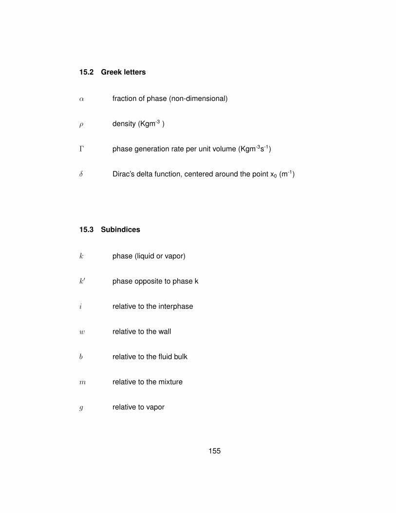
15.2 Greek letters
α fraction of phase (non-dimensional)
ρ density (Kgm-3 )
Γ phase generation rate per unit volume (Kgm-3s-1)
δ Dirac’s delta function, centered around the point x0 (m-1)
15.3 Subindices
k phase (liquid or vapor)
k′ phase opposite to phase k
i relative to the interphase
w relative to the wall
b relative to the fluid bulk
m relative to the mixture
g relative to vapor
155

f relative to liquid
156

16 Appendix RELAP 5 Model
=SMR Model1
2
3
*crdno problem type option4
0000100 new transnt5
*----------------------------------------------------------------6
*crdno inp-chk/run option7
0000101 run8
*----------------------------------------------------------------9
*crdno input units output units10
0000102 british british11
*12
*crdno end time min dt max dt ssd00 minor ed major ed restart13
0000201 600.0 1.0-6 0.01 0003 500 10000 1000014
*15
$$$$$$$$$$$$$$$$$$$$$$$$$$$$$$$$$$$$$$$$$$$$$$$$$$$$$$$$$$$$$$$$$16
$$$$$$$$$$$$$$$$$$$$$$$$$$$$$$$$$$$$$$$$$$$$$$$$$$$$$$$$$$$$$$$$$17
$18
$ Primary Loop19
$20
$$$$$$$$$$$$$$$$$$$$$$$$$$$$$$$$$$$$$$$$$$$$$$$$$$$$$$$$$$$$$$$$$21
$$$$$$$$$$$$$$$$$$$$$$$$$$$$$$$$$$$$$$$$$$$$$$$$$$$$$$$$$$$$$$$$$22
157

*23
$$$$$$$$$$$$$$$$$$$$$$$$$$$$$$$$$$$$$$$$$$$$$$$$$$$$$$$$$$$$$$$$$24
$25
$ COMPONENT 100- Lower Plenum26
$27
$$$$$$$$$$$$$$$$$$$$$$$$$$$$$$$$$$$$$$$$$$$$$$$$$$$$$$$$$$$$$$$$$28
*29
*crdno component name component type30
1000000 "LowPle" branch31
*32
*crdno number of junctions vel/flw33
1000001 4 134
*35
*crdno flowarea length volume36
1000101 41.2 2.2 0.037
*38
*crdno horz orient vert orient delta z39
1000102 0.0 -90.0 -2.240
*41
*till here geometry42
*43
*crdno roughness hyd. diameter fe44
1000103 0.00015 41.2 0045
*46
*crdno vol ic pressure eq temp47
1000200 003 1850.0 500.048
*49
* Junktions lower Plenum50
*51
158

*crdno from to area f loss r loss cahs52
1001101 100010001 110010001 4.9 0.0 0.0 000053
1002101 100010001 120010001 4.9 0.0 0.0 000054
1003101 500200002 100010001 12.85 0.0 0.0 000055
1004101 501200002 100010001 12.85 0.0 0.0 000056
*57
*crdno f flowrate g flowrate j flowrate58
1001201 647.2 0.0 0.059
1002201 647.2 0.0 0.060
1003201 647.2 0.0 0.061
1004201 647.2 0.0 0.062
*63
$$$$$$$$$$$$$$$$$$$$$$$$$$$$$$$$$$$$$$$$$$$$$$$$$$$$$$$$$$$$$$$$$64
$65
$ COMPONENT 110- Core Left66
$67
$$$$$$$$$$$$$$$$$$$$$$$$$$$$$$$$$$$$$$$$$$$$$$$$$$$$$$$$$$$$$$$$$68
*69
*crdno component name component type70
1100000 "Core" pipe71
*72
*crdno number of volumes73
1100001 874
*75
*crdno vol area vol.no.76
1100101 4.9 877
*78
*crdno length vol.no.79
1100301 1.0 780
159
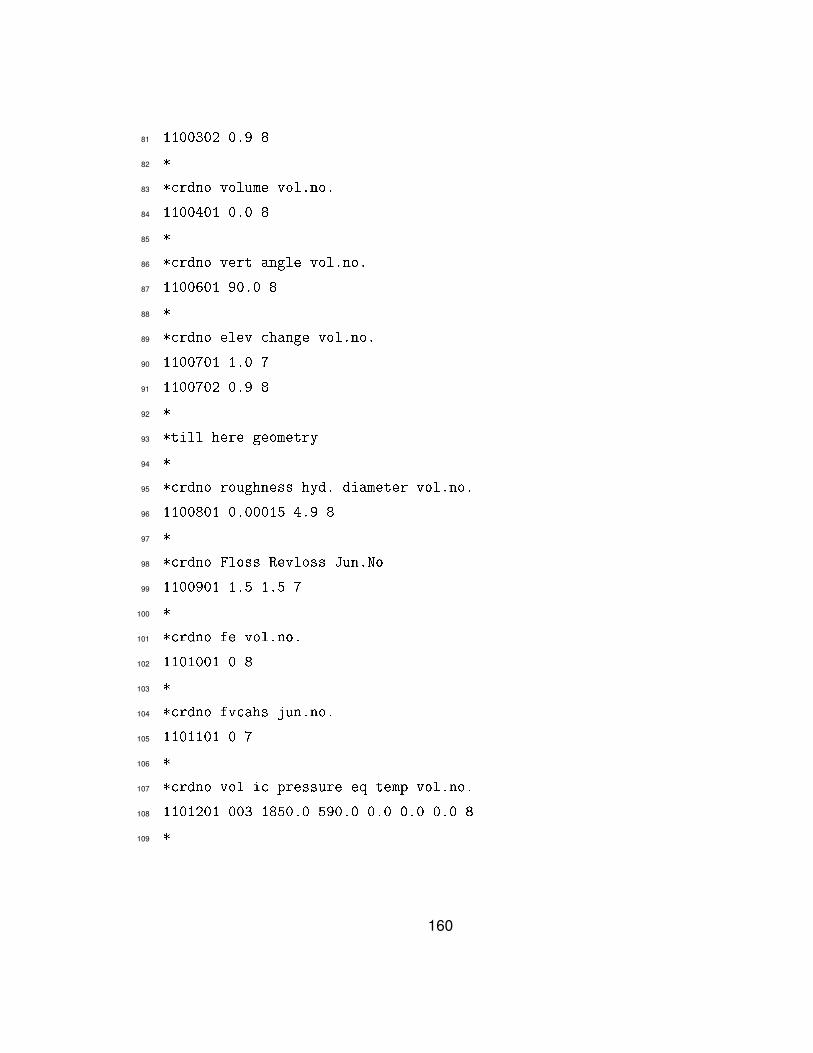
1100302 0.9 881
*82
*crdno volume vol.no.83
1100401 0.0 884
*85
*crdno vert angle vol.no.86
1100601 90.0 887
*88
*crdno elev change vol.no.89
1100701 1.0 790
1100702 0.9 891
*92
*till here geometry93
*94
*crdno roughness hyd. diameter vol.no.95
1100801 0.00015 4.9 896
*97
*crdno Floss Revloss Jun.No98
1100901 1.5 1.5 799
*100
*crdno fe vol.no.101
1101001 0 8102
*103
*crdno fvcahs jun.no.104
1101101 0 7105
*106
*crdno vol ic pressure eq temp vol.no.107
1101201 003 1850.0 590.0 0.0 0.0 0.0 8108
*109
160

*crdno makes lbm/s110
1101300 1111
*112
*crdno f flowrate g flowrate j flowrate jun.no.113
1101301 647.2 0.0 0.0 7114
*115
$$$$$$$$$$$$$$$$$$$$$$$$$$$$$$$$$$$$$$$$$$$$$$$$$$$$$$$$$$$$$$$$$116
$117
$ COMPONENT 120- Core Right118
$119
$$$$$$$$$$$$$$$$$$$$$$$$$$$$$$$$$$$$$$$$$$$$$$$$$$$$$$$$$$$$$$$$$120
*121
*crdno component name component type122
1200000 "Core" pipe123
*124
*crdno number of volumes125
1200001 8126
*127
*crdno vol area vol.no.128
1200101 4.9 8129
*130
*crdno length vol.no.131
1200301 1.0 7132
1200302 0.9 8133
*134
*crdno volume vol.no.135
1200401 0.0 8136
*137
*crdno vert angle vol.no.138
161

1200601 90.0 8139
*140
*crdno elev change vol.no.141
1200701 1.0 7142
1200702 0.9 8143
*144
*till here geometry145
*146
*crdno roughness hyd. diameter vol.no.147
1200801 0.00015 4.9 8148
*149
*crdno Floss Revloss Jun.No150
1200901 1.5 1.5 7151
*152
*crdno fe vol.no.153
1201001 0 8154
*155
*crdno fvcahs jun.no.156
1201101 0 7157
*158
*crdno vol ic pressure eq temp vol.no.159
1201201 003 1850.0 590.0 0.0 0.0 0.0 8160
*161
*crdno makes lbm/s162
1201300 1163
*164
*crdno f flowrate g flowrate j flowrate jun.no.165
1201301 647.2 0.0 0.0 7166
*167
162

$$$$$$$$$$$$$$$$$$$$$$$$$$$$$$$$$$$$$$$$$$$$$$$$$$$$$$$$$$$$$$$$$168
$169
$ COMPONENT 130- Core Left Riser Conection170
$171
$$$$$$$$$$$$$$$$$$$$$$$$$$$$$$$$$$$$$$$$$$$$$$$$$$$$$$$$$$$$$$$$$172
*173
**hydro component name component type174
1300000 "LeCoRiC" sngljun175
*176
*hydro from to area f loss r loss fvcahs177
1300101 110080002 200010001 4.9 0.0 0.0 0000178
*179
*crdno f flowrate g flowrate j flowrate180
1300201 1 647.2 0.0 0.0181
*182
$$$$$$$$$$$$$$$$$$$$$$$$$$$$$$$$$$$$$$$$$$$$$$$$$$$$$$$$$$$$$$$$$183
$184
$ COMPONENT 140- Core Right Riser Conection185
$186
$$$$$$$$$$$$$$$$$$$$$$$$$$$$$$$$$$$$$$$$$$$$$$$$$$$$$$$$$$$$$$$$$187
*188
*hydro component name component type189
1400000 "RiCoRiC" sngljun190
*191
*hydro from to area f loss r loss fvcahs192
1400101 120080002 200010001 4.9 0.0 0.0 0000193
*194
*crdno f flowrate g flowrate j flowrate195
1400201 1 647.2 0.0 0.0196
163
*197
$$$$$$$$$$$$$$$$$$$$$$$$$$$$$$$$$$$$$$$$$$$$$$$$$$$$$$$$$$$$$$$$$198
$199
$ COMPONENT 200- Lower Riser200
$201
$$$$$$$$$$$$$$$$$$$$$$$$$$$$$$$$$$$$$$$$$$$$$$$$$$$$$$$$$$$$$$$$$202
*203
*crdno component name component type204
2000000 "lowRise" pipe205
*206
*crdno number of volumes207
2000001 7208
*209
*crdno vol area vol.no.210
2000101 24.9 7211
*212
*crdno length vol.no.213
2000301 1.0 7214
*215
*crdno volume vol.no.216
2000401 0.0 7217
*218
*crdno vert angle vol.no.219
2000601 90.0 7220
*221
*crdno elev change vol.no.222
2000701 1.0 7223
*224
*till here geometry225
164
*226
*crdno roughness hyd. diameter vol.no.227
2000801 3.0 24.9 7228
*229
*finish till here230
*231
*crdno fe vol.no.232
2001001 0 7233
*234
*crdno fvcahs jun.no.235
2001101 0 6236
*237
*crdno vol ic pressure eq temp vol.no.238
2001201 003 1850.0 590.0 0.0 0.0 0.0 07239
*240
*crdno makes lbm/s241
2001300 1242
*243
*crdno f flowrate g flowrate j flowrate jun.no.244
2001301 1294.4 0.0 0.0 6245
*246
$$$$$$$$$$$$$$$$$$$$$$$$$$$$$$$$$$$$$$$$$$$$$$$$$$$$$$$$$$$$$$$$$247
$248
$ COMPONENT 205- Lower Middle Riser Connection249
$250
$$$$$$$$$$$$$$$$$$$$$$$$$$$$$$$$$$$$$$$$$$$$$$$$$$$$$$$$$$$$$$$$$251
*252
**hydro component name component type253
2050000 "LoMiRiC" sngljun254
165

*255
*hydro from to area f loss r loss fvcahs256
2050101 200070002 210010001 24.9 0.0 0.0 030000257
*258
*crdno f flowrate g flowrate j flowrate259
2050201 1 1294.4 0.0 0.0260
*261
$$$$$$$$$$$$$$$$$$$$$$$$$$$$$$$$$$$$$$$$$$$$$$$$$$$$$$$$$$$$$$$$$262
$263
$ COMPONENT 210- Middle Riser264
$265
$$$$$$$$$$$$$$$$$$$$$$$$$$$$$$$$$$$$$$$$$$$$$$$$$$$$$$$$$$$$$$$$$266
*267
*crdno component name component type268
2100000 "MidRise" pipe269
*270
*crdno number of volumes271
2100001 5272
*273
*crdno vol area vol.no.274
2100101 24.9 1275
2100102 22.525 2276
2100103 20.15 3277
2100104 17.775 4278
2100105 15.4 5279
*280
*crdno length vol.no.281
2100301 1.0 1282
2100302 1.0 2283
166

2100303 1.0 3284
2100304 1.0 4285
2100305 0.4 5286
*287
*crdno volume vol.no.288
2100401 0.0 5289
*290
*crdno vert angle vol.no.291
2100601 90.0 5292
*293
*crdno elev change vol.no.294
2100701 1.0 4295
2100702 0.4 5296
*297
*till here geometry298
*299
*crdno roughness hyd. diameter vol.no.300
2100801 0.00015 24.9 1301
2100802 0.00015 22.525 2302
2100803 0.00015 20.15 3303
2100804 0.00015 17.775 4304
2100805 0.00015 15.4 5305
*306
*finish till here307
*308
*crdno fe vol.no.309
2101001 0 5310
*311
*crdno fvcahs jun.no.312
167
2101101 0 4313
*314
*crdno vol ic pressure eq temp vol.no.315
2101201 003 1850.0 590.0 0.0 0.0 0.0 5316
*317
*crdno makes lbm/s318
2101300 1319
*320
*crdno f flowrate g flowrate j flowrate jun.no.321
2101301 1294.4 0.0 0.0 4322
*323
$$$$$$$$$$$$$$$$$$$$$$$$$$$$$$$$$$$$$$$$$$$$$$$$$$$$$$$$$$$$$$$$$324
$325
$ COMPONENT 215- Middle Upper Riser Connection326
$327
$$$$$$$$$$$$$$$$$$$$$$$$$$$$$$$$$$$$$$$$$$$$$$$$$$$$$$$$$$$$$$$$$328
*329
*hydro component name component type330
2150000 "MiUpRiC" sngljun331
*332
*hydro from to area f loss r loss fvcahs333
2150101 210050002 220010001 15.4 0.0 0.0 030000334
*335
*crdno f flowrate g flowrate j flowrate336
2150201 1 1294.4 0.0 0.0337
*338
$$$$$$$$$$$$$$$$$$$$$$$$$$$$$$$$$$$$$$$$$$$$$$$$$$$$$$$$$$$$$$$$$339
$340
$ COMPONENT 220- Upper Riser341
168

$342
$$$$$$$$$$$$$$$$$$$$$$$$$$$$$$$$$$$$$$$$$$$$$$$$$$$$$$$$$$$$$$$$$343
*344
*crdno component name component type345
2200000 "UpRise" pipe346
*347
*crdno number of volumes348
2200001 25349
*350
*crdno vol area vol.no.351
2200101 15.4 25352
*353
*crdno length vol.no.354
2200301 1.0 24355
2200302 0.81 25356
*357
*crdno volume vol.no.358
2200401 0.0 25359
*360
*crdno vert angle vol.no.361
2200601 90.0 25362
*363
*crdno elev change vol.no.364
2200701 1.0 24365
2200702 0.81 25366
*367
*till here geometry368
*369
*crdno roughness hyd. diameter vol.no.370
169

2200801 1.5 15.4 25371
*372
*finish till here373
*374
*crdno fe vol.no.375
2201001 0 25376
*377
*crdno fvcahs jun.no.378
2201101 0 24379
*380
*crdno vol ic pressure eq temp vol.no.381
2201201 003 1850.0 590.0 0.0 0.0 0.0 25382
*383
*crdno makes lbm/s384
2201300 1385
*386
*crdno f flowrate g flowrate j flowrate jun.no.387
2201301 1294.4 0.0 0.0 24388
*389
$$$$$$$$$$$$$$$$$$$$$$$$$$$$$$$$$$$$$$$$$$$$$$$$$$$$$$$$$$$$$$$$$390
$391
$ COMPONENT 350- Upper Plenum392
$393
$$$$$$$$$$$$$$$$$$$$$$$$$$$$$$$$$$$$$$$$$$$$$$$$$$$$$$$$$$$$$$$$$394
*395
*crdno component name component type396
3500000 "UppPlen" branch397
*398
*crdno number of junctions vel/flw399
170

3500001 4 1400
*401
*crdno flowarea length volume402
3500101 41.2 1.7 0.0403
*404
*crdno horz orient vert orient delta z405
3500102 0.0 90.0 1.7406
*407
*till here geometry408
*409
*crdno roughness hyd. diameter fe410
3500103 0.00015 41.2 00411
*412
*crdno volic pressure eq temp413
3500200 003 1850.0 590.0414
*415
* Junktions Upper Plenum416
*417
*crdno from to area f loss juncArea(r) loss cahs418
3501101 220250002 350010001 15.4 0.0 0.0 0000419
3502101 360010001 350010002 23.16 0.0 0.0 0000420
3503101 350010001 400010001 12.85 0.0 0.0 0000421
3504101 350010001 400010001 12.85 0.0 0.0 0000422
*423
*crdno f flowrate g flowrate j flowrate (flowrate)424
3501201 1294.4 0.0 0.0425
3502201 0.0 0.0 0.0426
3503201 647.2 0.0 0.0427
3504201 647.2 0.0 0.0428
171

*429
$$$$$$$$$$$$$$$$$$$$$$$$$$$$$$$$$$$$$$$$$$$$$$$$$$$$$$$$$$$$$$$$$430
$431
$ COMPONENT 360- Pressurizer432
$433
$$$$$$$$$$$$$$$$$$$$$$$$$$$$$$$$$$$$$$$$$$$$$$$$$$$$$$$$$$$$$$$$$434
*435
*crdno component name component type436
3600000 "WGIC" branch437
*438
*crdno number of junctions vel/flw439
3600001 1 1440
*441
*crdno flow area length volume442
3600101 0.0 1.6110 37.306443
*444
*crdno horz orient vert orient delta z445
3600102 0.0 90.0 1.6110446
*447
*crdno roughness hyd. diameter fe448
3600103 0.00015 0.0 00449
*450
*crdno vol ic pressure quality451
3600200 002 1850.0 0.7452
*453
* Junktions Water-Gas-Interface-Component454
*455
*crdno from to area f loss juncArea(r) loss cahs456
3601101 360010001 350010002 23.16 0.0 0.0 0000457
172

*458
*crdno f flowrate g flowrate j flowrate459
3601201 0.0 0.0 0.0460
*461
$$$$$$$$$$$$$$$$$$$$$$$$$$$$$$$$$$$$$$$$$$$$$$$$$$$$$$$$$$$$$$$$$462
$463
$ COMPONENT 400- Steam Generator Primary464
$465
$$$$$$$$$$$$$$$$$$$$$$$$$$$$$$$$$$$$$$$$$$$$$$$$$$$$$$$$$$$$$$$$$466
*467
*crdno component name component type468
4000000 "SGPri" pipe469
*470
*crdno number of volumes471
4000001 15472
*473
*crdno vol area vol.no.474
4000101 25.7 15475
*476
*crdno length vol.no.477
4000301 1.61 15478
*479
*crdno volume vol.no.480
4000401 0.0 15481
*482
*crdno vert angle vol.no.483
4000601 -90.0 15484
*485
*crdno elev change vol.no.486
173
4000701 -1.61 15487
*488
*crdno roughness hyd. diameter vol.no.489
4000801 0.00015 25.7 15490
*491
*crdno Floss Revloss Jun.No492
4000901 0.995 0.995 14493
*494
*crdno fe vol.no.495
4001001 0 15496
*497
*crdno fvcahs jun.no.498
4001101 0 14499
*500
*crdno vol ic pressure eq temp vol.no.501
4001201 003 1850.0 590.0 0.0 0.0 0.0 15502
*503
*crdno makes lbm/s504
4001300 1505
*506
*crdno f flowrate g flowrate j flowrate jun.no.507
4001301 1294.4 0.0 0.0 14508
*509
$$$$$$$$$$$$$$$$$$$$$$$$$$$$$$$$$$$$$$$$$$$$$$$$$$$$$$$$$$$$$$$$$510
$511
$ COMPONENT 405- SG Downcomer Conncetion 1512
$513
$$$$$$$$$$$$$$$$$$$$$$$$$$$$$$$$$$$$$$$$$$$$$$$$$$$$$$$$$$$$$$$$$514
*515
174

*hydro component name component type516
4050000 "SGDC1" sngljun517
*518
*hydro from to area f loss r loss fvcahs519
4050101 400150002 500010001 12.85 0.0 0.0 0000520
*521
*crdno f flowrate g flowrate j flowrate522
4050201 1 647.2 0.0 0.0523
*524
$$$$$$$$$$$$$$$$$$$$$$$$$$$$$$$$$$$$$$$$$$$$$$$$$$$$$$$$$$$$$$$$$525
$526
$ COMPONENT 406- SG Downcomer Conncetion 2527
$528
$$$$$$$$$$$$$$$$$$$$$$$$$$$$$$$$$$$$$$$$$$$$$$$$$$$$$$$$$$$$$$$$$529
*530
*hydro component name component type531
4060000 "SGDC2" sngljun532
*533
*hydro from to area f loss r loss fvcahs534
4060101 400150002 501010001 12.85 0.0 0.0 0000535
*536
*crdno f flowrate g flowrate j flowrate537
4060201 1 647.2 0.0 0.0538
539
$$$$$$$$$$$$$$$$$$$$$$$$$$$$$$$$$$$$$$$$$$$$$$$$$$$$$$$$$$$$$$$$$540
$541
$ COMPONENT 500- SG Downcomer 1542
$543
$$$$$$$$$$$$$$$$$$$$$$$$$$$$$$$$$$$$$$$$$$$$$$$$$$$$$$$$$$$$$$$$$544
175

*545
*crdno component name component type546
5000000 "downcom1" annulus547
*548
*crdno number of volumes549
5000001 20550
*551
*crdno vol area vol.no.552
5000101 12.85 20553
*554
*crdno length vol.no.555
5000301 1.0 19556
5000302 0.96 20557
*558
*crdno volume vol.no.559
5000401 0.0 20560
*561
*crdno vert angle vol.no.562
5000601 -90.0 20563
*564
*crdno elev change vol.no.565
5000701 -1.0 19566
5000702 -0.96 20567
*568
*till here geometry569
*570
*crdno roughness hyd. diameter vol.no.571
5000801 1.5 12.85 20572
*573
176

*finish till here574
*575
*crdno fe vol.no.576
5001001 0 20577
*578
*crdno cahs jun.no.579
5001101 0 19580
*581
*crdno vol ic pressure eq temp vol.no.582
5001201 003 1850.0 500.0 0.0 0.0 0.0 20583
*584
*crdno makes lbm/s585
5001300 1586
*587
*crdno f flowrate g flowrate j flowrate jun.no.588
5001301 647.2 0.0 0.0 19589
*590
$$$$$$$$$$$$$$$$$$$$$$$$$$$$$$$$$$$$$$$$$$$$$$$$$$$$$$$$$$$$$$$$$591
$592
$ COMPONENT 501- SG Downcomer 2593
$594
$$$$$$$$$$$$$$$$$$$$$$$$$$$$$$$$$$$$$$$$$$$$$$$$$$$$$$$$$$$$$$$$$595
*596
*crdno component name component type597
5010000 "downcom2" annulus598
*599
*crdno number of volumes600
5010001 20601
*602
177
*crdno vol area vol.no.603
5010101 12.85 20604
*605
*crdno length vol.no.606
5010301 1.0 19607
5010302 0.96 20608
*609
*crdno volume vol.no.610
5010401 0.0 19611
5010402 0.0 20612
*613
*crdno vert angle vol.no.614
5010601 -90.0 20615
*616
*crdno elev change vol.no.617
5010701 -1.0 19618
5010702 -0.96 20619
*620
*till here geometry621
*622
*crdno roughness hyd. diameter vol.no.623
5010801 1.5 12.85 20624
*625
*finish till here626
*627
*crdno fe vol.no.628
5011001 0 20629
*630
*crdno cahs jun.no.631
178

5011101 0 19632
*633
*crdno vol ic pressure eq temp vol.no.634
5011201 003 1850.0 500.0 0.0 0.0 0.0 20635
*636
*crdno makes lbm/s637
5011300 1638
*639
*crdno f flowrate g flowrate j flowrate jun.no.640
5011301 647.2 0.0 0.0 19641
*642
$$$$$$$$$$$$$$$$$$$$$$$$$$$$$$$$$$$$$$$$$$$$$$$$$$$$$$$$$$$$$$$$$643
$$$$$$$$$$$$$$$$$$$$$$$$$$$$$$$$$$$$$$$$$$$$$$$$$$$$$$$$$$$$$$$$$644
$645
$ Secondary Loop646
$647
$$$$$$$$$$$$$$$$$$$$$$$$$$$$$$$$$$$$$$$$$$$$$$$$$$$$$$$$$$$$$$$$$648
$$$$$$$$$$$$$$$$$$$$$$$$$$$$$$$$$$$$$$$$$$$$$$$$$$$$$$$$$$$$$$$$$649
*650
$$$$$$$$$$$$$$$$$$$$$$$$$$$$$$$$$$$$$$$$$$$$$$$$$$$$$$$$$$$$$$$$$651
$652
$ COMPONENT 740- Source Volume653
$654
$$$$$$$$$$$$$$$$$$$$$$$$$$$$$$$$$$$$$$$$$$$$$$$$$$$$$$$$$$$$$$$$$655
*656
*hydro component name component type657
7400000 "Source" tmdpvol658
*659
*hydro area length volume660
179

7400101 1.0e6 0.0 1.0e+06661
*662
*hydro horz angle vert angle delta z663
7400102 0.0 0.0 0.0664
*665
*hydro roughness hyd diam fe666
7400103 0.0 1.0e6 000667
*668
*hydro ic669
7400200 003670
*671
*hydro tdigit pressure temperature672
7400201 0.0 500.0 300.0673
*674
$$$$$$$$$$$$$$$$$$$$$$$$$$$$$$$$$$$$$$$$$$$$$$$$$$$$$$$$$$$$$$$$$675
$676
$ COMPONENT 750- Source Junction677
$678
$$$$$$$$$$$$$$$$$$$$$$$$$$$$$$$$$$$$$$$$$$$$$$$$$$$$$$$$$$$$$$$$$679
*680
*hydro component name component type681
7500000 "Tigflo" tmdpjun682
*683
*hydro from to area684
7500101 740010002 760010001 0.785685
*686
*hydro vel/flw trip no. alpha vrc numeric vrc687
7500200 1688
*689
180

*hydro t f flowrate g flowrate j flowrate690
7500201 0.0 0.0 0.0 0.0691
7500202 1.0 201.0 0.0 0.0692
*693
$$$$$$$$$$$$$$$$$$$$$$$$$$$$$$$$$$$$$$$$$$$$$$$$$$$$$$$$$$$$$$$$$694
$695
$ COMPONENT 760- Feed Water Pipe696
$697
$$$$$$$$$$$$$$$$$$$$$$$$$$$$$$$$$$$$$$$$$$$$$$$$$$$$$$$$$$$$$$$$$698
*699
*crdno component name component type700
7600000 "WatPip" pipe701
*702
*crdno number of volumes703
7600001 25704
*705
*crdno vol area vol.no.706
7600101 0.785 25707
*708
*crdno length vol.no.709
7600301 1.0 25710
*711
*crdno volume vol.no.712
7600401 0.0 25713
*714
*crdno vert angle vol.no.715
7600601 0.0 19716
7600602 45.0 20717
7600603 90.0 25718
181
*719
*crdno elev change vol.no.720
7600701 0.0 19721
7600702 0.5 20722
7600703 1.0 25723
*724
*till here geometry725
*726
*crdno roughness hyd. diameter vol.no.727
7600801 0.00015 0.785 25728
*729
*finish till here730
*731
*crdno fe vol.no.732
7601001 0 25733
*734
*crdno fvcahs jun.no.735
7601101 0 24736
*737
*crdno vol ic pressure eq temp vol.no.738
7601201 003 500.0 300.0 0.0 0.0 0.0 25739
*740
*crdno makes lbm/s741
7601300 1742
*743
*crdno f flowrate g flowrate j flowrate jun.no.744
7601301 147.81 0.0 0.0 24745
*746
$$$$$$$$$$$$$$$$$$$$$$$$$$$$$$$$$$$$$$$$$$$$$$$$$$$$$$$$$$$$$$$$$747
182

$748
$ COMPONENT 770- Feed Water Pipe SG Connection749
$750
$$$$$$$$$$$$$$$$$$$$$$$$$$$$$$$$$$$$$$$$$$$$$$$$$$$$$$$$$$$$$$$$$751
*752
*hydro component name component type753
7700000 "FWSG" sngljun754
*755
*hydro from to area f loss r loss fvcahs756
7700101 760250002 401010001 0.785 0.0 0.0 0000757
*758
*crdno f flowrate g flowrate j flowrate759
7700201 1 147.81 0.0 0.0760
*761
$$$$$$$$$$$$$$$$$$$$$$$$$$$$$$$$$$$$$$$$$$$$$$$$$$$$$$$$$$$$$$$$$762
$763
$ COMPONENT 401- Steam Generator Secondary764
$765
$$$$$$$$$$$$$$$$$$$$$$$$$$$$$$$$$$$$$$$$$$$$$$$$$$$$$$$$$$$$$$$$$766
*767
*crdno component name component type768
4010000 "SGSec" pipe769
*770
*crdno number of volumes771
4010001 15772
*773
*crdno vol area vol.no.774
4010101 0.785 15775
*776
183
*crdno length vol.no.777
4010301 1.61 15778
*779
*crdno volume vol.no.780
4010401 0.0 15781
*782
*crdno vert angle vol.no.783
4010601 90.0 15784
*785
*crdno elev change vol.no.786
4010701 1.61 15787
*788
*crdno roughness hyd. diameter vol.no.789
4010801 0.00015 0.785 15790
*791
*crdno fe vol.no.792
4011001 0 15793
*794
*crdno fvcahs jun.no.795
4011101 0 14796
*797
*crdno vol ic pressure eq temp vol.no.798
4011201 003 500.0 300.0 0.0 0.0 0.0 15799
*800
*crdno makes lbm/s801
4011300 1802
*803
*crdno f flowrate g flowrate j flowrate jun.no.804
4011301 147.81 0.0 0.0 14805
184

*806
$$$$$$$$$$$$$$$$$$$$$$$$$$$$$$$$$$$$$$$$$$$$$$$$$$$$$$$$$$$$$$$$$807
$808
$ COMPONENT 775- SG Steam Pipe Connection809
$810
$$$$$$$$$$$$$$$$$$$$$$$$$$$$$$$$$$$$$$$$$$$$$$$$$$$$$$$$$$$$$$$$$811
*812
*hydro component name component type813
7750000 "SGSP" sngljun814
*815
*hydro from to area f loss r loss fvcahs816
7750101 401150002 780010001 0.785 0.0 0.0 0000817
*818
*crdno f flowrate g flowrate j flowrate819
7750201 1 0.0 147.81 0.0820
*821
$$$$$$$$$$$$$$$$$$$$$$$$$$$$$$$$$$$$$$$$$$$$$$$$$$$$$$$$$$$$$$$$$822
$823
$ COMPONENT 780- Steam Pipe824
$825
$$$$$$$$$$$$$$$$$$$$$$$$$$$$$$$$$$$$$$$$$$$$$$$$$$$$$$$$$$$$$$$$$826
*827
*crdno component name component type828
7800000 "Steapi" pipe829
*830
*crdno number of volumes831
7800001 25832
*833
*crdno vol area vol.no.834
185

7800101 0.785 25835
*836
*crdno length vol.no.837
7800301 1.0 25838
*839
*crdno volume vol.no.840
7800401 0.0 25841
*842
*crdno vert angle vol.no.843
7800601 90.0 5844
7800602 45.0 6845
7800603 0.0 25846
*847
*crdno elev change vol.no.848
7800701 1.0 5849
7800702 0.5 6850
7800703 0.0 25851
*852
*till here geometry853
*854
*crdno roughness hyd. diameter vol.no.855
7800801 0.00015 0.785 25856
*857
*finish till here858
*859
*crdno fe vol.no.860
7801001 0 25861
*862
*crdno fvcahs jun.no.863
186

7801101 0 24864
*865
*crdno vol ic pressure eq temp vol.no.866
7801201 003 500.0 575.0 0.0 0.0 0.0 25867
*868
*crdno makes lbm/s869
7801300 1870
*871
*crdno f flowrate g flowrate j flowrate jun.no.872
7801301 0.0 147.81 0.0 24873
*874
$$$$$$$$$$$$$$$$$$$$$$$$$$$$$$$$$$$$$$$$$$$$$$$$$$$$$$$$$$$$$$$$$875
$876
$ COMPONENT 790- Steam Pipe Sink Connection877
$878
$$$$$$$$$$$$$$$$$$$$$$$$$$$$$$$$$$$$$$$$$$$$$$$$$$$$$$$$$$$$$$$$$879
*880
*hydro component name component type881
7900000 "SPSIC" sngljun882
*883
*hydro from to area f loss r loss fvcahs884
7900101 780250002 800010001 0.785 0.0 0.0 00000885
*886
*hydro f flowrate g flowrate j flowrate887
7900201 1 0.0 147.81 0.0888
*889
$$$$$$$$$$$$$$$$$$$$$$$$$$$$$$$$$$$$$$$$$$$$$$$$$$$$$$$$$$$$$$$$$890
$891
$ COMPONENT 800- Sink892
187

$893
$$$$$$$$$$$$$$$$$$$$$$$$$$$$$$$$$$$$$$$$$$$$$$$$$$$$$$$$$$$$$$$$$894
*895
*hydro component name component type896
8000000 "Sink" tmdpvol897
*898
*hydro area length volume899
8000101 1.0e6 0.0 1.0e+06900
*901
*hydro horz angle vert angle delta z902
8000102 0.0 0.0 0.0903
*904
*hydro roughness hyd diam fe905
8000103 0.0 1128.378 000906
*907
*hydro ic908
8000200 0002909
*910
*hydro tdigit pressure temp911
8000201 0.0 500.0 0.999912
*913
$$$$$$$$$$$$$$$$$$$$$$$$$$$$$$$$$$$$$$$$$$$$$$$$$$$$$$$$$$$$$$$$$914
$$$$$$$$$$$$$$$$$$$$$$$$$$$$$$$$$$$$$$$$$$$$$$$$$$$$$$$$$$$$$$$$$915
$916
$ Accident Valve917
$918
$$$$$$$$$$$$$$$$$$$$$$$$$$$$$$$$$$$$$$$$$$$$$$$$$$$$$$$$$$$$$$$$$919
$$$$$$$$$$$$$$$$$$$$$$$$$$$$$$$$$$$$$$$$$$$$$$$$$$$$$$$$$$$$$$$$$920
*921
188

*crdno Name Type922
*9550000 "Accvlv" valve923
*924
*hydro from to area f loss r loss fvcahs925
*9550101 400080003 401080004 12.99 0.0 0.0 0926
*927
*crdno f flowrate g flowrate j flowrate928
*9550201 1 0.0 0.0 0.0929
*930
*crdno Valvetype931
*9550300 trpvlv932
*933
*crdno TripNumber934
*9550301 401935
*936
$$$$$$$$$$$$$$$$$$$$$$$$$$$$$$$$$$$$$$$$$$$$$$$$$$$$$$$$$$$$$$$$$937
$ Trip938
$$$$$$$$$$$$$$$$$$$$$$$$$$$$$$$$$$$$$$$$$$$$$$$$$$$$$$$$$$$$$$$$$939
*940
0000401 time 0 gt null 0 5001. l941
*942
$$$$$$$$$$$$$$$$$$$$$$$$$$$$$$$$$$$$$$$$$$$$$$$$$$$$$$$$$$$$$$$$$943
$$$$$$$$$$$$$$$$$$$$$$$$$$$$$$$$$$$$$$$$$$$$$$$$$$$$$$$$$$$$$$$$$944
$945
$ Heat Structures946
$947
$$$$$$$$$$$$$$$$$$$$$$$$$$$$$$$$$$$$$$$$$$$$$$$$$$$$$$$$$$$$$$$$$948
$$$$$$$$$$$$$$$$$$$$$$$$$$$$$$$$$$$$$$$$$$$$$$$$$$$$$$$$$$$$$$$$$949
*950
189

$$$$$$$$$$$$$$$$$$$$$$$$$$$$$$$$$$$$$$$$$$$$$$$$$$$$$$$$$$$$$$$$$951
$952
$ COMPONENT 1820- Steam Generator Tubes953
$954
$$$$$$$$$$$$$$$$$$$$$$$$$$$$$$$$$$$$$$$$$$$$$$$$$$$$$$$$$$$$$$$$$955
*956
*crdno heat str-s mesh pts geometry init flag left coord957
18201000 15 3 1 1 0.024958
*959
*crdno mesh locn flag mesh fmt flag960
18201100 0 1961
962
*crdno no.intervals rt.coord963
18201101 2 0.026964
*965
*crdno comp no. interval no.966
18201201 001 2967
*968
*crdno source value mesh int. no.969
18201301 0.0 2970
*971
*crdno Initialtempflag972
18201400 0973
*974
*crdno temperature mesh pt no.975
18201401 560.0 3976
*977
*crdno left volume incr b.cond sa code area/factor ht str no.978
18201501 400010000 10000 1 1 1350.2 15979
190

*980
*crdno rt volume incr b.cond sa code area/factor ht str no.981
18201601 401150000 -10000 1 1 1350.2 15982
*983
*crdno s. type s. mult left heat right heat ht str no.984
18201701 0 0.0 0.0 0.0 15985
*986
*finish till here987
*988
*crdno con.val989
18201800 0990
*991
*ADD LEFT BOUNDARY CONDITION992
*crdno equiv diam heated len's grid len's grid cf's bf ht strno993
18201801 0.285 50.0 50.0 0.0 0.0 0.0 0.0 1.0 15994
*995
*crdno con.val996
18201900 0997
*998
*ADD RIGHT BOUNDARY CONDITION999
*crdno equiv diam heated len's grid len's grid cf's bf ht str no.1000
18201901 5.2e-2 50.0 50.0 0.0 0.0 0.0 0.0 1.0 151001
*1002
$$$$$$$$$$$$$$$$$$$$$$$$$$$$$$$$$$$$$$$$$$$$$$$$$$$$$$$$$$$$$$$$$1003
$1004
$ COMPONENT 1810- Fuel Rods1005
$1006
$$$$$$$$$$$$$$$$$$$$$$$$$$$$$$$$$$$$$$$$$$$$$$$$$$$$$$$$$$$$$$$$$1007
*1008
191

*crdno heat str-s mesh pts geometry init flag left coord1009
18101000 8 2 1 1 0.01010
*1011
*crdno MeshLocation MeshFormat1012
18101100 0 11013
*1014
*crdno no. intervals rt. coord1015
18101101 1 0.03121016
*1017
*crdno comp no. interval no.1018
18101201 005 11019
*1020
*crdno source value mesh int. no.1021
18101301 1.0 11022
*1023
*crdno Initialtempflag1024
18101400 01025
*1026
*crdno temperature mesh pt no.1027
18101401 590.0 21028
*1029
*crdno left volume incr b.cond sa code area/factor ht str no.1030
18101501 120010000 10000 1 0 392.14 81031
*1032
*crdno rt volume incr b.cond sa code area/factor ht str no.1033
18101601 110010000 10000 1 0 392.14 81034
*1035
*crdno s. type s. mult left heat right heat ht str no.1036
18101701 100 0.125 0.0 0.0 81037
192

*1038
*finish till here1039
*1040
*crdno con.val1041
18101800 01042
*1043
*ADD LEFT BOUNDARY CONDITION1044
*crdno equiv diam heated len's grid len's grid cf's bf ht str no.1045
18101801 0.041 50.0 50.0 0.0 0.0 0.0 0.0 1.0 81046
*1047
*crdno con.val1048
18101900 01049
*1050
*ADD RIGHT BOUNDARY CONDITION1051
*crdno equiv diam heated len's grid len's grid cf's bf ht str no.1052
18101901 0.041 50.0 50.0 0.0 0.0 0.0 0.0 1.0 81053
*1054
*crdno Tabletype Trip Factors1055
20210000 power1056
*1057
*crdno t[s] P[MW] per Heat Struc.1058
20210001 0.0 0.01059
20210002 1.0 125.01060
20210003 160.0 125.01061
20210004 700.0 140.01062
20210005 1000.0 160.01063
*1064
$$$$$$$$$$$$$$$$$$$$$$$$$$$$$$$$$$$$$$$$$$$$$$$$$$$$$$$$$$$$$$$$$1065
$$$$$$$$$$$$$$$$$$$$$$$$$$$$$$$$$$$$$$$$$$$$$$$$$$$$$$$$$$$$$$$$$1066
193
$1067
$ Tables1068
$1069
$$$$$$$$$$$$$$$$$$$$$$$$$$$$$$$$$$$$$$$$$$$$$$$$$$$$$$$$$$$$$$$$$1070
$$$$$$$$$$$$$$$$$$$$$$$$$$$$$$$$$$$$$$$$$$$$$$$$$$$$$$$$$$$$$$$$$1071
*1072
*Thermal Propertiels for heat structures1073
*1074
*=*=*=*=*=*=*=*=*=*=*=*=*=*=*=*=*=*=*=*=*=*=*=*=***1075
* thermal properties of ss-316l - composition 1 *1076
*=*=*=*=*=*=*=*=*=*=*=*=*=*=*=*=*=*=*=*=*=*=*=*=*1077
*1078
*crdno mtrl type th.con ht.cap material1079
20100100 tbl/fctn 1 1 * ss-316l1080
*1081
* thermal properties of ss-316l1082
*1083
*crdno temperature th.cond1084
20100101 32.0 0.002151085
20100102 100.0 0.002151086
20100103 800.0 0.003061087
20100104 1600.0 0.003971088
20100105 3600.0 0.003971089
*1090
*crdno temperature vol ht cap1091
20100151 32.0 61.301092
20100152 400.0 61.301093
20100153 600.0 64.601094
20100154 800.0 67.101095
194

20100155 1000.0 69.351096
20100156 4000.0 69.351097
*1098
*=*=*=*=*=*=*=*=*=*=*=*=*=*=*=*=*=*=*=*=*=*=*=*=*=*=1099
* thermal properties of cladding - composition 4 *1100
*=*=*=*=*=*=*=*=*=*=*=*=*=*=*=*=*=*=*=*=*=*=*=*=*=*=1101
*1102
*crdno mtrl type th.con ht.cap material1103
20100400 tbl/fctn 1 1 * cladding1104
*1105
* thermal properties of cladding1106
*1107
*crdno temperature th.cond1108
20100401 32. 1.9267e-31109
20100402 392.0 1.9267e-31110
20100403 752.0 2.2478e-31111
20100404 1112.0 2.7297e-31112
20100405 1472.0 3.0508e-31113
20100406 1832.0 3.5325e-31114
20100407 2192.0 4.0142e-31115
20100408 2552.0 4.8169e-31116
20100409 2912.0 5.7803e-31117
20100410 3272.0 7.0647e-31118
20100411 3632.0 8.8311e-31119
20100412 3992.0 1.0918e-21120
*1121
*crdno temperature vol ht cap1122
20100451 0.0 28.3921123
20100452 1480.3 34.4761124
195

20100453 1675.00 85.1761125
20100454 1787.5 34.3701126
20100455 3500.0 34.4761127
*1128
*1129
*=*=*=*=*=*=*=*=*=*=*=*=*=*=*=*=*=*=*=*=*=*=***1130
* thermal properties of uo2 - composition 5 *1131
*=*=*=*=*=*=*=*=*=*=*=*=*=*=*=*=*=*=*=*=*=*=***1132
*1133
*crdno mtrl type th.con ht.cap material1134
20100500 tbl/fctn 1 1 * uo21135
*1136
* thermal properties of uo21137
*1138
*crdno temperature th.cond1139
20100501 32.0 1.284e-31140
20100502 188.6 1.284e-31141
20100503 332.6 1.1235e-31142
20100504 440.6 9.951e-41143
20100505 500.0 9.2806e-41144
20100506 650.0 7.4194e-41145
20100507 800.0 7.4361e-41146
20100508 897.0 5.8390e-41147
20100509 1104.0 5.2310e-41148
20100510 1213.0 4.9200e-41149
20100511 1326.0 4.6710e-41150
20100512 1684.0 4.4700e-41151
20100513 1700.0 4.4701e-41152
20100514 1850.0 4.5528e-41153
196

20100515 2000.0 4.3556e-41154
20100516 2150.0 4.1861e-41155
20100517 2300.0 4.0472e-41156
20100518 2450.0 3.9306e-41157
20100519 2600.0 3.8389e-41158
20100520 3100.0 3.6750e-41159
20100521 3600.0 3.7028e-41160
20100522 4100.0 3.9056e-41161
20100523 4600.0 4.2722e-41162
20100524 5100.0 4.8056e-41163
*1164
*crdno temperature vol ht cap1165
20100551 32.0 34.451166
20100552 122.0 38.351167
20100553 212.0 40.951168
20100554 392.0 43.551169
20100555 752.0 46.801170
20100556 2012.0 51.351171
20100557 2732.0 52.651172
20100558 3092.0 56.551173
20100559 3452.0 63.051174
20100560 3812.0 72.801175
20100561 4352.0 89.701176
20100562 4532.0 94.251177
20100563 4712.0 98.151178
20100564 4892.0 100.101179
20100565 5144.0 101.401180
20100566 8000.0 101.401181
*1182
197

*=*=*=*=*=*=*=*=*=*=*=*=*=*=*=*=*=*=*=*=*=*=*=*=*=*=*=*=*=*=*=*=**1183
* thermal properties of fuel gap(average core) - composition 6 *1184
*=*=*=*=*=*=*=*=*=*=*=*=*=*=*=*=*=*=*=*=*=*=*=*=*=*=*=*=*=*=*=*=**1185
*1186
*crdno mtrl type th.con ht.cap material1187
20100600 tbl/fctn 1 1 * fuel gap1188
*1189
* thermal properties of fuel gap1190
*1191
*crdno temperature th.cond1192
20100601 32.0 0.000311193
20100602 5400.0 0.000311194
*1195
*crdno temperature vol ht cap1196
20100651 32.0 0.0000751197
20100652 5400.0 0.0000751198
*1199
. end of case1200
198
Bibliography
[1] Sebastian Buchholz, Anne Krüssenberg, Andreas Schaffrath, and Reinhard
Zipper. Studie zur Sicherheit und zu internationalen Entwicklungen von Small
Modular Reactors (SMR): Abschlussbericht, volume 376 of GRS. Gesellschaft
für Anlagen- und Reaktorsicherheit (GRS) gGmBH, Köln, Mai 2015.
[2] International Atomic Energy Agency. Instrumentation and control systems for
advanced small modular reactors: International atomic energy agency. IAEA
nuclear energy series, 2017.
[3] International Atomic Energy Agency. Options to enhance proliferation resis-
tance of innovative small and medium sized reactors: International atomic en-
ergy agency. IAEA nuclear energy series, 2014.
[4] John OHara. Human-performance issues related to the design and operation
of small modular reactors. June 2012.
199

[5] U.S. GOVERNMENT. An examination of the safety and economics of light
water small modular reactors. July 14, 2011.
[6] U.S. GOVERNMENT. Illustration of a light water small modular nuclear reactor
(smr), 24. August 2015.
[7] Nuclear technology basics: Part 8 liquid metal cooled reactors:
http://neurovoresnuclearnetworknews.blogspot.com/2011/07/part-8-liquid-
metal-cooled-reactors.html, 2011.
[8] World Nuclear Association. Small nuclear power reactors - world nuclear asso-
ciation, November 2017.
[9] Molten salt reactors: https://steemit.com/science/@anarchyhasnogods/molten-
salt-reactors, 2017.
[10] Hans-Dieter Berger. Nukleare energietechnik i: Umdruck und vorlesung. Tech-
nische Universität Braunschweig, 2016.
[11] Robert Howard Shannon and Henry C. Schwenk. Nuclear Power Engineering.
2012.
[12] John R. Lamarsh and Anthony John Baratta. Introduction to Nuclear Engineer-
ing. Pearson Education, Inc, Hoboken, NJ, fourth edition edition, 2018.
200

[13] CLP Group. Pressurised water reactor vs boiling water reactor:
https://www.clpgroup.com/nuclearenergy/eng/power/power4_1_2.aspx, 2013.
[14] Thomas Schabbach and Viktor Wesselak. Energie: Die Zukunft wird erneuer-
bar. SpringerLink Bücher. Springer Vieweg, Berlin and Heidelberg, 2012.
[15] Dieter Smidt. Reaktor-Sicherheitstechnik. Springer Berlin Heidelberg, Berlin,
Heidelberg, 1979.
[16] Paul Laufs. Reaktorsicherheit für Leistungskernkraftwerke: Die Entwicklung im
politischen und technischen Umfeld der Bundesrepublik Deutschland. Springer,
Berlin and Heidelberg, 2013.
[17] Günter Kessler, Anke Veser, Franz-Hermann Schlüter, Wolfgang Raskob, Clau-
dia Landman, and Jürgen Päsler-Sauer. Sicherheit von Leichtwasserreaktoren:
Risiken der Nukleartechnologie. Springer, Berlin and Heidelberg, 2012.
[18] The Asia Pacific Journal. Out of the shadows: Can japan’s nuclear power
renaissance reduce global emissions?, September 1, 2008.
[19] Jose Reyes. Nuscale plant safety in response to extreme events. Nuclear
Technology, 2012.
201
[20] NuScale Power. Smr nuclear technology: http://www.nuscalepower.com/,
2007.
[21] Vundela Siva, Reddy, Subash Chndra, Kaushik, Sudhir Kumar, Tyagi, Narayan-
lal, and Panwar. An approach to analyse energy and exergy analysis of thermal
power plants: A review, 2010.
[22] Hans Dieter Baehr and Stephan Kabelac. Thermodynamik: Grundlagen und
technische Anwendungen. SpringerLink Bücher. Springer Vieweg, Berlin, Hei-
delberg, 15. auflage edition, 2012.
[23] Bernhard Weigand, Jürgen Köhler, and Jens von Wolfersdorf. Thermodynamik
kompakt. Springer-Lehrbuch. Springer Berlin Heidelberg, Berlin, Heidelberg
and s.l., 3., aktual. aufl. 2013 edition, 2013.
[24] Karl Strauß. Wärmekraftwerke: Von den Anfängen im 19. Jahrhundert bis zur
Endphase ihrer Entwicklung. Springer Vieweg, Berlin and Heidelberg, 2016.
[25] Heinz Pitsch. Thermodynamik i rwth aachen: Kapitel 5, teil 1. 2012.
[26] Carl Pfleiderer and Hartwig Petermann. Strömungsmaschinen. Klassiker der
Technik. Springer, Berlin, 7., unveränd. aufl. edition, 2005.
[27] The RELAP5-3D c© Code Development Team. Relap5-3d c© code manuel vol-
202
ume i: Code structure, system models, and solution methods: Volume i. Idaho
National Laboratory, April 2005.
[28] The RELAP5-3D c© Code Development Team. Relap5-3d c© code manual vol-
ume ii: User’s guide and input requirements: Volume ii. Idaho National Labora-
tory, April 2005.
[29] The RELAP5-3D c© Code Development Team. Relap5-3d c© code manual vol-
ume iv: Models and correlations: Volume iv. Idaho National Laboratory, Febru-
ary 2001.
[30] SCDAP/RELAP5-3D c© Code Development Team. Scdap/relap5-3d c© code
manual volume iii: User’s guide and input manual: Volume iii. Idaho National
Engineering and Environmental Laboratory, October 2003.
[31] R. R. Schultz. Relap5-3d c© code manual volume v: User’s guidelines: Volume
v. July 2002.
[32] U.S. Nuclear Regulatory Commission. Development of a computer tool for in-
depth analysis and post processing of the relap5 thermal hydraulic code. April
2011.
[33] Christopher Earls Brennen. Thermo-Hydraulics of Nuclear Reactors. Cam-
bridge University Press, Cambridge, 2016.
203

[34] Mamoru Ishii and Takashi Hibiki. Thermo-Fluid Dynamics of Two-Phase Flow.
Smart energy systems–nanowatts to terawatts. Springer Science+Business
Media Inc, Boston, MA, 2006.
[35] Hiroyasu MOCHIZUKI. Thermal-hydraulics in nuclear reactors: International
graduate course tokyo institute of technology. October 2009.
[36] Mamoru Ishii. Investigation of Natural Circulation Instability and Transients in
Passively Safe Small Modular Reactors: Reactor Concepts Research Develop-
ment and Demonstration. 2016.
[37] Yoram ZVIRIN. A review of natural circulation loops in pressurized water reak-
tors and other systems. Electric Power Research Institute, 1981.
[38] International Atomic Energy Agency. Natural circulation in water cooled nuclear
power plants: Phenomena, models, and methodology for system reliability as-
sessments. November 2005.
[39] Japan Atomic Energy Agency. Residual heat removal using buoyancy force:
http://jolisfukyu.tokai-sc.jaea.go.jp/fukyu/review_en/2011/1_3.html, 2011.
[40] Andreas Bott. Synoptische Meteorologie: Methoden der Wetteranalyse und
-prognose. Springer, Berlin, 2012.
204
[41] Albert Ziegler and Hans-Josef Allelein. Reaktortechnik: Physikalisch-
technische Grundlagen. Springer, Berlin, 2., beu bearb. aufl. 2013 edition,
2013.
[42] Herbert Oertel, Martin Böhle, and Ludwig Prandtl. Prandtl - Führer durch die
Strömungslehre: Grundlagen und Phänomene. Springer Fachmedien Wies-
baden, Wiesbaden and s.l., 13., überarb. aufl. 2012 edition, 2012.
[43] NuScale Inc. Final safety analysis report - part 02 - tier 02 - chapter 05 - reactor
coolant system and connecting systems. 2016.
[44] NuScale Inc. Final safety analysis report - part 02 - tier 02 - chapter 10 - steam
and power conversion system. 2016.
[45] NuScale Inc. Final safety analysis report - part 02 - tier 02 - chapter 04 - reactor.
2016.
205