Embed Size (px)
Citation preview

EXPLORATION ENGINEERING
Transient pressure analysis for vertical oil exploration wells:a case of Moga field
Azza Hashim Abbas1 • Wan Rosli Wan Sulaiman1 • Mohd Zaidi Jaafar1 •
Agi Augustine Aja1
Received: 16 September 2016 / Accepted: 24 April 2017 / Published online: 1 June 2017
� The Author(s) 2017. This article is an open access publication
Abstract Reservoir engineers use the transient pressure
analyses to get certain parameters and variable factors on
the reservoir’s physical properties, such as permeability
thickness, which need highly sophisticated equipments,
methods and procedures. The problem facing the explo-
ration and production teams, with the discoveries of new
fields, is the insufficiency of accurate and appropriate data
to work with due to different sources of errors. The well-
test analyst does the work without reliable set of data from
the field, thus, resulting in many errors, which may con-
sequently cause damage and unnecessary financial losses,
as well as opportunity losses to the project. This paper
analyzes and interprets the noisy production rate and
pressure data with problematic mechanical damage using a
deconvolution method. Deconvolution showed improve-
ment in simulation results in detecting the boundaries.
Also, high-risk area analysis with different methods being
applied to get the best set of results needed for subsequent
operations.
Keywords Well test � Transient pressure analysis �Simulation � Convolution � Deconvolution
List of symbols
q Volumetric flow rate (m3/s)
h Reservoir permeability (m)
k Formation permeability (m2)
P Reservoir pressure (psi)
l Dynamic viscosity of fluid (cp)
c Compressibility of fluid (psi)
q Density of fluid (kg/m3)
T Temperature
t Time, (days)
Dt Time increment (sec)
Pi Initial reservoir pressure (Psi)
pwf Flowing well pressure, (STB\D)
q Fluid density, gm
cm3
rRe External radius, (ft)
rw Wellbore radius, (ft)
m Slope of semi-log line, (Psi/cycle)
S Skin factor
p� Homer extrapolated pressure
PI Jð Þ Productivity index STB/D (Psi)
Abbreviations
API American Petroleum Institute
PI Productivity index
SPE Society of Petroleum Engineers
STB Stock tank barrel
IPR Inflow performance relationship
PVT Pressure volume temperature
Introduction
Well tests have been widely used for several decades in the
oil industry to estimate reservoir properties, such as initial
pressure, fluid type, permeability and identification of
reservoir barriers/boundaries in the formation volume near
the wellbore (Pitzer 1964). Information collected during
well testing usually consists of flow rates, pressure patterns,
temperature data and fluid samples (Sulaiman and Hashim
2016).
& Wan Rosli Wan Sulaiman
1 Department of Petroleum Engineering, Faculty of Chemical
and Energy Engineering, Universiti Teknologi Malaysia,
UTM Skudai, 81310 Johor Bahru, Malaysia
123
J Petrol Explor Prod Technol (2018) 8:521–529
https://doi.org/10.1007/s13202-017-0352-0

Well-testing operation in new fields is faced difficulties
such as geological complex that requires advanced tech-
nology (Wiebe 1980), experienced personnel and longer
durations for operations. Operator companies regularly
developing new fields without extensive evaluation of the
predicted reserves and the actual (Bittencourt and Horne
1997). Therefore, different reservoir engineer needs to be
careful in interpreting the routine drill string test (DST),
(Dean and Petty 1964; Oliver and Chen 2011). There is no
single method of testing and sampling, that is, the best for
the purpose under every circumstance (Soh 2010; Whittle
et al. 2003). The selection of the test type, sequence and
duration has to be balanced against operational risk, geol-
ogy, environmental constraints, equipment and the eco-
nomic value derived from affecting early decisions on
project appraisal or development (Bottomley et al. 2015; Li
et al. 2014).
There are several sources of uncertainties in the analyses
and interpretations of well-test data (Ballin et al. 1993;
Sulaiman and Hashim 2016; Vargas et al. 2015; Bittencourt
and Horne 1997) as follows:
• Physical errors in the pressure data, such as noise drift
temperature effects and time shift.
• Errors in the flow rate measurement.
• The non-unique response of the reservoir with the
production time effects.
• Uncertainty of rock and fluid properties.
Routine well-test analysis provides data on the average
properties of the reservoir near the well, but does not
provide the overall reservoir characteristics and bound-
aries. One of the main reasons for this limitation is that a
traditional well-test analysis handles the transient pressure
data collected from a single well over a short duration. For
instance, log and modular formation dynamic tester (MDT)
data only provide information on areas adjacent to the
wellbore, while the seismic data cannot delineate the
heterogeneity of the reservoir (Ballin et al. 1993; Khale-
dialidusti et al. 2015).
The Moga field is located in the west of Sudan and was
discovered at the beginning of 2003. It was a promising
location but with a lot of risks, such as the uncontrolled
movement of armed and rebellious tribes during the
expected process of drilling and completion, the geological
nature of the land and the heterogeneity of the petrological
layers. These led to a situation where a standard DST
operation was carried out for three days without a design
for the operation sequence, which should have been based
on the field situational characteristics.
Drilling the first well was difficult, costly and ended
with abandonment of the well due to lost circulation of oil.
Various types of measures were taken during drilling of a
test borehole in the second well, (Well 22) which was
performed as an exploratory well aimed at the mid-lower
Abu Gabra formation at the proposed depth of 2700 mKB
and was safely completed. However, the high mud density
caused extensive damage to the nearer well area, which
also distracted the hypothetical oil rate of flow that does not
represent the real reservoir characteristics, burdened with
additional risk of poor test design for testing time and huge
pressure noise. In view of this anomaly, it is not logical to
consider that the test cannot be saved from being run on an
inappropriate source of data.
The well-test analyst does the work without going
through well-informed and reliable data from different
sources, thus resulting in many errors, which may conse-
quently lead to misleading parameters affecting the total
estimation of reserves, which will eventually lead to
financial loss to the company.
In this paper, the production rate and pressure data from
a noisy Gauge were analyzed by joining two gauges and a
new pressure profile was generated from the confidence
interval. The results were analyzed using the convolution
and deconvolution method to extract the skin factor, pro-
ductivity index and average permeability, which solved the
problem of defining the exact reservoir boundaries and
offers more advantages in the analysis, especially in future
development plan and reduction in the noise data effect at
the initial stage.
Literature review
The calculated result on damaged exploratory petrological
entities using the deconvolution simulation can be quite
challenging compared to the convolution simulation, but on
the other hand, the boundary identification can also be
quite misleading by using the regular (convolution) simu-
lation, which should appropriately be performed through
the deconvolution method. Using a deconvolution method
in a high-risk area, like (Moga) field, offers more advan-
tages in the analysis, especially in future development
plans and reduction in the noise data effect in the initial
stage.
Convolution method
The details of convolution will be explained in a short
review of the physical principle of the methods that can
estimate the reservoir properties based on the multiple flow
periods being the principle of superposition. The principle
of superposition is similar to convolution and uses the
assumed linearity of the reservoir and the known step
response of the system, and it is possible to compute the
pressure response of the multiple flow periods by super-
positioning the known step responses. Convolution is used
522 J Petrol Explor Prod Technol (2018) 8:521–529
123

to calculate the pressure response based on any flow rate
function in a known system.
Bourdet (2002) presented a major development in the
mid-1980 in which he advocated superimposing of the log-
time derivative of the storage and skin solution on the
accepted form of the storage type curve. Combination of
the two types of curves could lead to a unique match of
field data, which could do away with the need for a Horner
buildup graph. They also observed that the data taken
before a semi-log straight line could be interpreted, as is
often the case, initial claims on this new method were not
entirely correct, as some major advantages of a derivative
graph were not yet evident. The first impression on the
derivative procedure was that the high-precision data were
initially required to make such a procedure feasible. The
solution to this was to first develop good numerical pro-
cedures to differentiate and categorize the numerous field
data. To date, the Bourdon-type data taken in the 1960s as
well as the high-precision liquid-level data and gas-purged
capillary tube data have been successfully differentiated.
One final important step made since 1976 concerns the
computer-aided interpretation. The various types of curves
and semi-log graphs involved in well-test analyses and
differentiation of field data were perfectly suited to a
computer with the appropriate software.
Deconvolution method
In general, the terms deconvolution is the inverse of con-
volution is used to calculate the output of a system, when
the input and the system dynamics often described by the
impulse response are known, whereas deconvolution can
be used to calculate the impulse response when the input
signals and output signals are known. The aim of decon-
volution is to calculate the impulse response of the system,
based on the transient pressure response and the flow rate.
In well-testing literature, there are, however, various defi-
nitions of deconvolution used. All the definitions are based
on the methods used to extract the impulse response g
(t) based on the input and output. However, deconvolution
which is the inverse of convolution is not always applied in
the practical sense of it. Sometimes, estimating the step
response h (t) of the system is also considered deconvo-
lution. A skilled engineer can eventually get the same
answers on deconvolution problems by using a regular
analysis (convolution method) (Xiaohu et al. 2010) and can
still give a direct view of the underlying model controlling
the well, thus getting the right answer faster. It provides the
equivalent radius-of-investigation for the test.
In the field of well testing, deconvolution is considered
as a reliable tool to estimate the shut-in pressure response
of the reservoir during a varying flow rate (Vaferi and
Eslamloueyan 2015). This technique improves the
estimation of the type of curve needed, by reshaping the
data, which readily improves the estimation of the reservoir
properties (Horne and Liu 2013; Liu and Horne 2013).
Since 1999, several research works have been carried out
on deconvolution in the field of well testing. There is a lot
of attention given to deconvolution in the field of well
testing (Gringarten 2010; Gringarten 2006; Houze et al.
2010; Levitan 2007; Onur et al. 2009).
Methodology
Well and reservoir overview
Based on the drilling data source and completion program,
this test was to estimate the skin factor and initial reservoir
pressure in this area, which was needed for the next drilling
operations (Table 1).
Well-testing reservoir parameter
Well testing is conducted to obtain data for interpretation
of the reservoirs characteristics, average parameters
including porosity, permeability, pressure, temperature,
depths, oil viscosity and GOR, all of which are needed to
be identified or assumed as the case may be and this data
are gathered by the geologist for testing at the PVT labo-
ratory to obtain the expected results.
The input data from well reports of geologist, fluid
properties and completion reports are summarized in
Table 2. In the case of (Abu Gabra), the reservoir is
homogeneous. Therefore, assumption is isotropic of con-
stant thickness.
The study was focused on Well-22 especially, on the
Drill Stem Test in the Abu Gabra reservoir because it was
the first well to be completed and its production time was
very short. As such careful attention was focused on
choosing the appropriate sequence of analysis to work
with.
Result and discussion
Convolution analysis
The previous data were plotted using the simulator; the
cartesian plot of (pressure vs time) and (Pressure difference
vs time) was generated by the simulator.
By loading pressure gauges data, it can be seen that the
noise distracted the first area as shown in Fig. 1.
Two gauges were loaded with the green points, which
are referred to the basic gauge, and the orange points,
which are referred to the back-up gauge. The presence of
J Petrol Explor Prod Technol (2018) 8:521–529 523
123
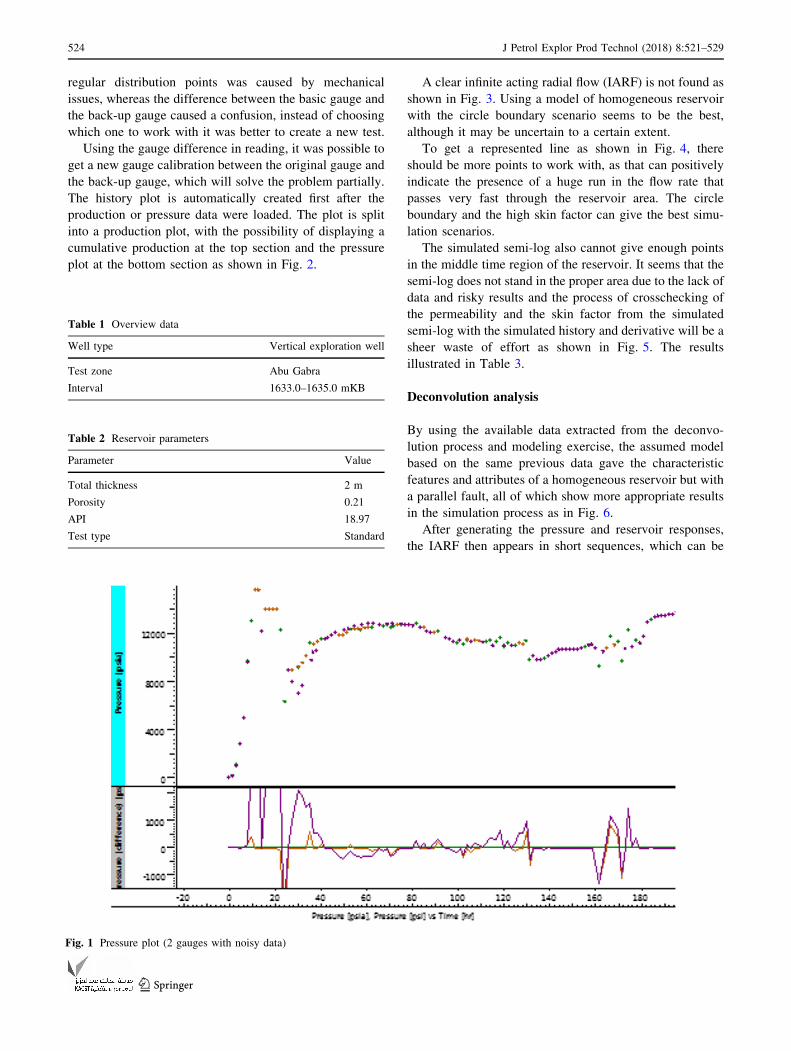
regular distribution points was caused by mechanical
issues, whereas the difference between the basic gauge and
the back-up gauge caused a confusion, instead of choosing
which one to work with it was better to create a new test.
Using the gauge difference in reading, it was possible to
get a new gauge calibration between the original gauge and
the back-up gauge, which will solve the problem partially.
The history plot is automatically created first after the
production or pressure data were loaded. The plot is split
into a production plot, with the possibility of displaying a
cumulative production at the top section and the pressure
plot at the bottom section as shown in Fig. 2.
A clear infinite acting radial flow (IARF) is not found as
shown in Fig. 3. Using a model of homogeneous reservoir
with the circle boundary scenario seems to be the best,
although it may be uncertain to a certain extent.
To get a represented line as shown in Fig. 4, there
should be more points to work with, as that can positively
indicate the presence of a huge run in the flow rate that
passes very fast through the reservoir area. The circle
boundary and the high skin factor can give the best simu-
lation scenarios.
The simulated semi-log also cannot give enough points
in the middle time region of the reservoir. It seems that the
semi-log does not stand in the proper area due to the lack of
data and risky results and the process of crosschecking of
the permeability and the skin factor from the simulated
semi-log with the simulated history and derivative will be a
sheer waste of effort as shown in Fig. 5. The results
illustrated in Table 3.
Deconvolution analysis
By using the available data extracted from the deconvo-
lution process and modeling exercise, the assumed model
based on the same previous data gave the characteristic
features and attributes of a homogeneous reservoir but with
a parallel fault, all of which show more appropriate results
in the simulation process as in Fig. 6.
After generating the pressure and reservoir responses,
the IARF then appears in short sequences, which can be
Table 1 Overview data
Well type Vertical exploration well
Test zone Abu Gabra
Interval 1633.0–1635.0 mKB
Table 2 Reservoir parameters
Parameter Value
Total thickness 2 m
Porosity 0.21
API 18.97
Test type Standard
Fig. 1 Pressure plot (2 gauges with noisy data)
524 J Petrol Explor Prod Technol (2018) 8:521–529
123

Fig. 2 History plot (pressure,
rate vs. time)
Fig. 3 Simulated derivative-
type curve for circle scenario
Fig. 4 Simulated semi-log
J Petrol Explor Prod Technol (2018) 8:521–529 525
123

detected easily from the chosen reservoir area that provides
better results on the reservoir characteristic properties for
gainful usage at a later stage.
Figures 7 and 8 show a yellow line, which represents the
reservoir, where the change in the flat line indicates a
structural shape, in this case, a parallel fault with no flow
boundary. The results are shown in Table 4.
Discussion
Tables 3 and 4 show the characteristic fracture damage.
The change in the determined values of skin (s) between
the convolution and deconvolution estimated to be 4.3%
from the average which can be neglected in practical
aspects. The variation in range of the initial reservoir
pressure between the two methods is within accept-
able limit. However, the reservoir permeability cannot be
obtained from the convolution process because the data do
not represent the extended reservoir area. The results show
reduction in the permeability up to 20% which is beyond
the accepted range of practical errors. On the other hand,
the deconvolution method has given a better result, after
using the condition of a parallel fault even though it does
not give a very close result with the circle result. It is to be
noted that the convolution method can yield a very wrong
estimate of the boundary identity, whereas the deconvo-
lution technique can be more useful in the boundary
identity. To accept the deconvolution technique results, a
discreet consideration should be evaluated in retrospect of
the past well history with the lost circulation, whereas the
application of the convolution method needs more time
stages to reduce the rate of flow by changing the choke
size. Furthermore, the convolution method cannot truly
forecast the reservoir capacity because the damage in the
stimulation has created an assumption of a higher flow rate
in excess of the reservoir actual capacity.
Conclusion
In this study, transient pressure analysis for vertical well
was conducted using Saphir Simulator. The techniques
introduced in this work give excellent estimation for
Fig. 5 Simulated history plot
for circle scenario
Table 3 Convolution simulated results
Property Value
Pi 14.155 kpa
S -3.81
Ko 21.6
526 J Petrol Explor Prod Technol (2018) 8:521–529
123

information of flow characteristics, as well as oil explo-
ration areas of uncertainty such as the interpretation of
preferred targeted oil thickness, wrong estimation of skin
factor, overestimation of productivity index.
The uncertainty factors associated with the noisy pres-
sure gauges were reduced after using the deconvolution
technique. However, it can be considerably mitigated if
calculated option can be made for other dip exploration
well by estimating the existence of the nearest fault and
heterogeneity change for each layer.
Recommendation
Further research works should be developed for the anal-
yses of long-term production data from exploration wells
and the present deconvolution analysis concepts should be
extended to include the rest of the wells. The use of the
deconvolution technique can produce better results, with
compatible views on the real boundary identity, as the
common usage of the regular technique has frequently been
quite misleading in terms of reservoir properties, especially
Fig. 6 Deconvolution
derivative plot
Fig. 7 Semi-log for
deconvolution analysis
J Petrol Explor Prod Technol (2018) 8:521–529 527
123

permeability which can be ranged using other logs to get a
better view.
Acknowledgements The authors would like to acknowledge Petro-
Energy Company Sudan for providing the data set.
Open Access This article is distributed under the terms of the
Creative Commons Attribution 4.0 International License (http://
creativecommons.org/licenses/by/4.0/), which permits unrestricted
use, distribution, and reproduction in any medium, provided you give
appropriate credit to the original author(s) and the source, provide a
link to the Creative Commons license, and indicate if changes were
made.
References
Ballin P, Aziz K, Journel A, Zuccolo L (1993) Quantifying the impact
of geological uncertainty on reservoir performing forecasts. In:
SPE symposium on reservoir simulation, Society of Petroleum
Engineers
Bittencourt AC, Horne RN (1997) Reservoir development and design
optimization. In: SPE annual technical conference and exhibi-
tion, Society of Petroleum Engineers
Bottomley W, Schouten J, McDonald E, Cooney T (2015) Novel well
test design for the evaluation of complete well permeability and
productivity for CSG wells in the Surat Basin. In: SPE Asia
pacific unconventional resources conference and exhibition,
Society of Petroleum Engineers
Bourdet D (2002) Well test analysis the use of advanced interpre-
tation models handbook of petroleum exploration & production,
vol 3. Elsevier, Amsterdam
Dean J, Petty L (1964) Making more complete use of Dst data. Log
Anal 5(03)
Gringarten AC (2006) From straight lines to deconvolution: the
evolution of the state-of-the art in well test analysis. In: SPE
annual technical conference and exhibition, Society of Petroleum
Engineers
Gringarten AC (2010) Practical use of well-test deconvolution. In:
SPE annual technical conference and exhibition, Society of
Petroleum Engineers
Horne RN, Liu Y (2013) Interpreting pressure and flow rate data from
permanent downhole gauges using convolution-Kernel-based
data mining approaches. In: SPE western regional & AAPG
pacific section meeting 2013 joint technical conference, Society
of Petroleum Engineers
Houze OP, Tauzin E, Allain OF (2010) New methods to deconvolve
well-test data under changing well conditions. In: SPE annual
technical conference and exhibition, Society of Petroleum
Engineers
Khaledialidusti R, Enayatpor S, Badham SJ, Carlisle CT, Kleppe J
(2015) An innovative technique for determining residual and
current oil saturations using a combination of log-inject-log and
SWCT test methods: LIL-SWCT. J Petrol Sci Eng 135:618–625
Levitan MM (2007) Deconvolution of multiwell test data. SPE J
12:420–428
Li Y, Li X, Teng S, Wang F, Xu D (2014) A new changing wellbore
storage model for pressure oscillation in pressure buildup test.
J Nat Gas Sci Eng 19:350–357
Liu Y, Horne R (2013) Interpreting pressure and flow rate data from
permanent downhole gauges with convolution-Kernel-based data
mining approaches. In: Paper SPE 166440 presented at the SPE
annual technical conference and exhibition, New Orleans
Oliver DS, Chen Y (2011) Recent progress on reservoir history
matching: a review. Comput Geosci 15:185–221
Fig. 8 Deconvolution
simulated history plot for
parallel fault with no flow
scenario
Table 4 Deconvolution simulation results
Property Value
Pi 13.892 kpa
S -3.98
Ko 26.6
528 J Petrol Explor Prod Technol (2018) 8:521–529
123

Onur M, Ayan C, Kuchuk FJ (2009) Pressure-pressure deconvolution
analysis of multi-well interference and interval pressure transient
tests. In: International petroleum technology conference, Inter-
national Petroleum Technology Conference
Pitzer S (1964) Uses of transient pressure tests. In: Drilling and
production practice, American Petroleum Institute, Washington
Soh MT (2010) Hydrocarbon liquid fraction mapping functions for
gas-condensate well test evaluation. J Petrol Sci Eng 73:185–193
Sulaiman WRW, Hashim A (2016) Cyclic steam stimulation effect on
skin factor reviewed case study. In: Applied mechanics and
materials, 2016. Trans Tech Publications pp 287–290
Vaferi B, Eslamloueyan R (2015) Hydrocarbon reservoirs character-
ization by co-interpretation of pressure and flow rate data of the
multi-rate well testing. J Petrol Sci Eng 135:59–72
Vargas R, Lira-Galeana C, Silva D, Manero O (2015) Inflow
performance of wells intersecting long fractures with transient
pressure and variable flow-rate behavior. J Petrol Sci Eng
136:23–31
Whittle T, Lee J, Gringarten A (2003) Will wireline formation tests
replace well tests? In: SPE annual technical conference and
exhibition, Society of Petroleum Engineers
Wiebe M (1980) Piper field: geology. In: European offshore
technology conference and exhibition, Society of Petroleum
Engineers
Xiaohu H, Shiyi Z, Xiangfang L (2010) Studies on application of
deconvolution to multi-well interference test. Well Test 2:004
J Petrol Explor Prod Technol (2018) 8:521–529 529
123