Embed Size (px)
Citation preview
Ecological Modelling 185 (2005) 283–297
Transient population dynamics: Relations to lifehistory and initial population state
David N. Koonsa, ∗, James B. Grandb, Bertram Zinnerc, Robert F. Rockwelld
a Alabama Cooperative Fish and Wildlife Research Unit, School of Forestry and Wildlife Sciences,108 M. White Smith Hall, Auburn University, AL 36849, USA
b USGS Alabama Cooperative Fish and Wildlife Research Unit, School of Forestry and Wildlife Sciences,108 M. White Smith Hall, Auburn University, AL 36849, USA
c Department of Discrete and Statistical Sciences, 120 Math Annex, Auburn University, AL 36849, USAd Department of Ornithology, American Museum of Natural History, New York, NY 10024, USA
Received 19 July 2004; received in revised form 10 December 2004; accepted 13 December 2004
Abstract
Most environments are variable and disturbances (e.g., hurricanes, fires) can lead to substantial changes in a population’sstate (i.e., age, stage, or size distribution). In these situations, the long-term (i.e., asymptotic) measure of population growthrate (λ1) may inaccurately represent population growth in the short-term. Thus, we calculated the short-term (i.e., transient)population growth rate and its sensitivity to changes in the life-cycle parameters for three bird and three mammal species withwidely varying life histories. Further, we performed these calculations for initial population states that spanned the entire range
rowth
of theroducing
species.wildlifestate, or
gy7;
ula-
of possibilities. Variation in a population’s initial net reproductive value largely explained the variation in transient grates and their sensitivities to changes in life-cycle parameters (all AICc ≥ 6.67 units better than the null model, allR2 ≥ 0.55).Additionally, the transient fertility and adult survival sensitivities tended to increase with the initial net reproductive valuepopulation, whereas the sub-adult survival sensitivity decreased. Transient population dynamics of long-lived, slow repspecies were more variable and more different than asymptotic dynamics than they were for short-lived, fast reproducingBecauseλ1 can be a biased estimate of the actual growth rate in the short-term (e.g., 19% difference), conservation andbiologists should consider transient dynamics when developing management plans that could affect a population’swhenever population state could be unstable.Published by Elsevier B.V.
Keywords:Age structure; Demography; Life history; Sensitivity; Transient dynamics
∗ Corresponding author. Tel.: +1 334 8449267;fax: +1 334 8874509.
E-mail addresses:[email protected] (D.N. Koons),[email protected] (J.B. Grand), [email protected](B. Zinner), [email protected] (R.F. Rockwell).
1. Introduction
Sensitivity analysis has become popular in ecolo(e.g.,van Groenendael et al., 1988; Horvitz et al., 199Benton and Grant, 1999; Heppell et al., 2000a) andhas been used to manage and conserve wild pop
0304-3800/$ – see front matter. Published by Elsevier B.V.doi:10.1016/j.ecolmodel.2004.12.011

284 D.N. Koons et al. / Ecological Modelling 185 (2005) 283–297
tions (e.g.,Rockwell et al., 1997; Cooch et al., 2001;Fujiwara and Caswell, 2001). Such analyses usually as-sume that the population’s state (i.e., the age, stage, orsize distribution) remains stable through time (i.e., theasymptotic stable state), and that the population growsaccording to a constant, or stable distribution of rate(s)(e.g.,λ1, r, λs, a). All else being equal, theory suggeststhat the stable state assumption in population biology isa safe one (Lopez, 1961; Cull and Vogt, 1973; Cohen,1976, 1977a,b, 1979; Tuljapurkar, 1984, 1990).
Environmental catastrophes, natural disturbances,selective harvest regimes, and animal release and relo-cation programs can significantly alter a population’sstate, causing unstable states. When a population’sstate is not stable, it will change until the stable stateis reached. Meanwhile, the population dynamics are‘transient’ because they change according to the chang-ing population state until the asymptotic stable state isachieved. Empirical evidence suggests that stable pop-ulation states rarely occur in nature (Bierzychudek,1999; Clutton-Brock and Coulson, 2002). Thus, theassumption of asymptotic population dynamics in thewild may be unwarranted in many cases (Hastings andHiggins, 1994; Fox and Gurevitch, 2000; Hastings,2001, 2004).
Although much is known about the mathematicsof transient dynamics (Coale, 1972; Keyfitz, 1972;Trussell, 1977; Tuljapurkar, 1982), few have focusedon the demographic causes of transient change in pop-ulation size or growth rate even though they are theu bi-o
thef org cun-d ve-m ratea onet izea( ns t be-c thanar tew op-u e tog 0;
Yearsley, 2004). Thus, asymptotic sensitivities mightnot be informative for making management prescrip-tions in the immediate future.
We examine the sensitivity of ‘transient populationgrowth rate’ to changes in vital rates for six bird andmammal species across all possible population states.Our primary objective is to elucidate the biological cor-relates of intraspecific variation in transient dynamicsacross the possible population states. Our secondaryobjective is to explain variation in transient dynamicsacross life histories. Long-lived birds and mammalstend to have longer generation lengths and larger dis-parity in reproductive value across age classes. We hy-pothesize that these properties will cause the transientdynamics in long-lived species to be more variable anddifferent than asymptotic dynamics compared to short-lived, fast reproducing species.
2. Methods
2.1. Data sets and matrix projection models
To examine the magnitude of difference betweentransient dynamics and asymptotic dynamics acrossspecies, we chose three bird and three mammal speciesthat have been extensively studied and were known tohave widely varying life histories across the slow–fastcontinuum. Along the slow–fast continuum of bird andmammal life histories, the ‘slowest’ species are thosethat live a long life, mature late, and have low repro-d test’s re-p ensuG
ub-l s( s( tac 1s ,1 s( 97( aves avem hoehS al
nifying parameters of evolutionary and populationlogy (Sibly et al., 2002).
Sensitivity analysis can be used to determineunctional relationship between population sizerowth rate and the constituent vital rates (e.g., feity, survival, growth, maturation, recruitment, moent), and to project changes in population growthnd size as vital rates change. New tools allow
o examine the sensitivity of transient population snd structure (Fox and Gurevitch, 2000) or growth rateYearsley, 2004) to changes in the initial populatiotate or the vital rates. These new tools are importanause transient sensitivities may be very differentsymptotic sensitivities. For example, inCoryphanthaobbinsorum, the asymptotic population growth raas most sensitive to adult survival, but transient plation growth rate and size were most sensitivrowth of juvenile stages (Fox and Gurevitch, 200
uctive rates and long generation lengths. The ‘faspecies are short-lived, mature early, have highroductive rates and short generation lengths (saillard et al., 1989; Charnov, 1993).We attained age-specific vital-rate data from p
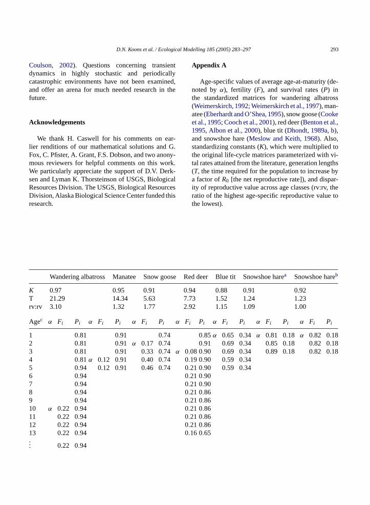
ished long-term studies of blue titParus caeruleuDhondt, 1989a,b), manatee Trichechus manatuEberhardt and O’Shea, 1995), red deer (Benton el., 1995; Albon et al., 2000), snow gooseChenaerulescens(Cooke et al., 1995; Cooch et al., 200),nowshoe hareLepus americanus(Meslow and Keith968), and wandering albatrossDiomedea exulanWeimerskirch, 1992; Weimerskirch et al., 19)Appendix A). Wandering albatross and manatee hlow life histories, snow goose and red deer hedium-slow life histories, and blue tit and snowsare have fast life histories (Heppell et al., 2000b;æther and Bakke, 2000). We used age-specific vit
D.N. Koons et al. / Ecological Modelling 185 (2005) 283–297 285
rates where the authors report age-specific differences.Meslow and Keith (1968)did not detect age-specificdifferences in vital rates during their long-term study.To examine the effects of age-structured vital rates ontransient dynamics in a fast species, we usedMeslowand Keith’s (1968)original data, and implemented
hypothetical age structure by increasing fertility by 5%for age 2 and 10% for ages 3 and older (Appendix A).
For each species, we assumed birth-pulse reproduc-tion and parameterized the vital-rate data into a life-cycle projection matrix (A) assuming a pre-breedingcensus
A =
0 · · · Fα · · · Fα+n−1 Fα+n
P1 0 0 · · · 0 0
0... 0 · · · 0 0
0 0 Pα · · · 0 0... 0
......
......
0 0 0 · · · Pα+n−1 Pα+n
(1)
whereα is the average age of first breeding and (α +n)is the oldest known age group with unique vital rates.B singp glep xb te
2
wthr
G
w tev ea rateft y of
the transient GR to infinitely small changes in a vital-rate (TSij ), which can be defined as,
TSij = ∂(∑
knt,k/∑
knt−1,k
)∂aij
. (3)
The solution of TSij is a two-part equation as fol-lows,
TSij =
e′∆ijn0
e′n0for t = 1
∑t−2l=0e
′Al∆ijAt−l−2(An0e′ − n0e′A)At−1n0 + e′At−1∆ijn0e′At−1n0
(e′At−1n0)2
for t = 2, 3, . . .
and derivation of the solution can be found inAppendixB, where we further provide explanation of notationand the similarities and differences of our derivation toYearsley (2004).
2.3. Simulations and projection analysis
For each life-cycle matrix, we attained the stablepopulation state vector and systematically generated1000 state vectors, each normalized to one (1200 forwandering albatross because of the larger state vectordimension), by systematically drawing numbers from arandom uniform distribution. To examine transient dy-namics under stable population state and random initialconditions, we projected each life-cycle matrix five-time steps (years) with each state vector using Eq.(B.1)(i.e., 1201 initial condition state vector projections forw ). Toc itions r, weu
∆
w i-t pec-ti arei ion-a ectora ouldh -iv thant
ecause the dynamics of increasing and decreaopulations can be very different, even within a sinopulation (Mertz, 1971), we multiplied each matriy a constantK (Appendix A) so that the dominanigenvalue of each matrix would be 1.00.
.2. Transient sensitivity analysis
For a population at any state, the population groate (GR) can be defined as,
R =∑
knt,k∑knt−1,k
(2)
herent, k is thek-th element of the population staector at timet. Thus, if the population is not in thsymptotic stable state, GR is the transient growth
or a one time step interval (seeAppendix Bfor longerime steps). We sought a solution to the sensitivit
andering albatross and 1001 for all other speciesalculate the distance between each initial condtate vector and the stable population state vectosedKeyfitz’s ∆ (1968),
(x, w1) = 1
2
∑k
|xk − w1,k| (4)
herexk and w1,k are thek-th elements of the inial population state and stable state vectors, resively. The maximum value of Keyfitz’s∆ is 1 andts minimum is 0 when the population state vectorsdentical. A population state vector that has proporttely more breeding adults than the stable state vnd one that has proportionately more sub-adults cave the same∆ value. To rectify this important biolog
cal difference, we assigned (+) values to all∆’s whenectors had proportionately more breeding adultshe stable state vector and (−) values to all∆’s when
286 D.N. Koons et al. / Ecological Modelling 185 (2005) 283–297
vectors had proportionately more sub-adults than thestable state vector. Species that mature and breed atage 1 (i.e., blue tit and snowshoe hare), and are countedwith a pre-breeding census, will not have sub-adults inthe population state vector. Thus, the signed Keyfitz∆ can only vary between 0 and 1 for these species.We used the signed Keyfitz∆ as a predictor variable instatistical analyses, and linearly mapped∆ values fromthe region [−1, 1] to the region [0, 2] in order to exam-ine models using the exponential distribution, whichranges from 0 to infinity. In addition, we calculated theinitial net reproductive value (c1) of a population foreach population state vector as,
c1 = v′1 × n0 (5)
wherev′1 is the dominant left eigenvector of theA ma-
trix normalized to 1 and represents state-specific repro-ductive value (Goodman, 1968).
Furthermore, we estimated the transient growth rateat time steps 1-to-2 (GR2), 4-to-5 (GR5), and 0-to-5(5YRGR). 5YRGR is not the usual measure of growthrate, but rather a measure of the percentage changein population size over 5 years. Additionally, we esti-mated the sensitivity of transient GR to small changesin the vital rates at time steps 1-to-2 and 4-to-5 ac-cording to Eq.(B.7). We then summed the transientsensitivity estimates across relevant state classes to ob-tain transient fertility sensitivity (TFS), transient sub-adult-survival sensitivity (TSASS), and transient adults mes ,wa tantKe
2
forw eciesa earm eent vari-a SS,a ps).B tran-s tions ares
(IRLS) robust regression with the Huber weight func-tion (Rousseeuw and Leroy, 1987; Carroll and Ruppert,1988; Neter et al., 1996: 418) to estimate the intraspe-cific relationships. Analyses were conducted with ProcNLIN (SAS Institute, Inc. 2000).
We used Akaike’s information criterion adjustedfor sample size (AICc) and Akaike weights (Akaike,1973; Burnham and Anderson, 1998: 51, 124) toevaluate the amount of support in our data for eachmodel in our candidate list (see above). We consideredthe best approximating model to be that with thelowest AICc value and highest Akaike weight (Wi )(Burnham and Anderson, 1998).
To examine the magnitude of difference betweentransient and asymptotic population dynamics for eachof the seven life histories, we first measured the differ-ence between each transient dynamic (e.g., GR2, TFS2,etc.) and the respective asymptotic dynamic for all sim-ulated projections. We then took the absolute value ofthe difference, and finally estimated the mean and vari-ance of the absolute values across all simulated projec-tions (1001, 1201 for wandering albatross) for each lifehistory. We again used IRLS robust regression with theHuber weight function to estimate the linear relation-ship between the generation length of the life history(explanatory variable) and each of the aforementioned‘difference’ estimates (response variable) (Rousseeuwand Leroy, 1987). We used F-tests to examine thesupport, or lack thereof, for the a priori hypothesis thatthe mean and variance of each ‘difference’ estimatew lifeh
3
ninem els)t blep tivev s toi ctst ureda thes life-c thata ther on
urvival sensitivity (TASS) for the aforementioned titeps (e.g.,Oli and Zinner, 2001: 383). For comparisone also estimated the asymptotic growth rate (λ1 = 1 inll cases after adjusting each life-cycle with a cons, Appendix A) and sensitivities (Caswell, 1978) forach life history.
.4. Data analysis
We used data from the 1001 projections (1201andering albatross) described above for each spnd considered a variety of null, linear, and nonlinodels to examine the form of the relationship betw
he initial net reproductive value and the responsebles describing transient dynamics (GR, TFS, TSAnd TASS at each of the aforementioned time steecause heteroscedasticity was present in theient response variables across the initial populatates, we used iteratively re-weighted least squ
ould increase with the generation length of theistory (Neter et al., 1996).
. Results
For each intraspecific analysis, we examinedodels (i.e., the null, linear, and nonlinear mod
o identify how departures away from the staopulation state affect the initial net reproducalue of a population, and another nine modeldentify how the initial net reproductive value afferansient dynamics. Transient dynamics meast the annual time scale did not exist in any ofimulations conducted for the snowshoe hareycle without age-structured vital rates, meaningsymptotic dynamics always occurred. However,esults for all other life-cycles and initial populati
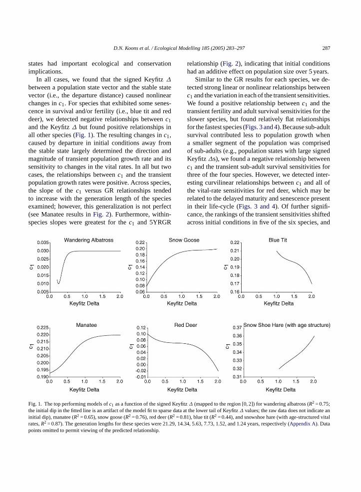
D.N. Koons et al. / Ecological Modelling 185 (2005) 283–297 287
states had important ecological and conservationimplications.
In all cases, we found that the signed Keyfitz∆
between a population state vector and the stable statevector (i.e., the departure distance) caused nonlinearchanges inc1. For species that exhibited some senes-cence in survival and/or fertility (i.e., blue tit and reddeer), we detected negative relationships betweenc1and the Keyfitz∆ but found positive relationships inall other species (Fig. 1). The resulting changes inc1,caused by departure in initial conditions away fromthe stable state largely determined the direction andmagnitude of transient population growth rate and itssensitivity to changes in the vital rates. In all but twocases, the relationships betweenc1 and the transientpopulation growth rates were positive. Across species,the slope of thec1 versus GR relationships tendedto increase with the generation length of the speciesexamined; however, this generalization is not perfect(see Manatee results inFig. 2). Furthermore, within-species slopes were greatest for thec1 and 5YRGR
relationship (Fig. 2), indicating that initial conditionshad an additive effect on population size over 5 years.
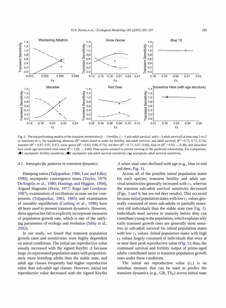
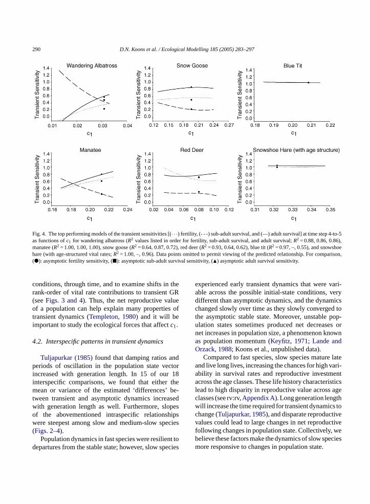
Similar to the GR results for each species, we de-tected strong linear or nonlinear relationships betweenc1 and the variation in each of the transient sensitivities.We found a positive relationship betweenc1 and thetransient fertility and adult survival sensitivities for theslower species, but found relatively flat relationshipsfor the fastest species (Figs. 3 and 4). Because sub-adultsurvival contributed less to population growth whena smaller segment of the population was comprisedof sub-adults (e.g., population states with large signedKeyfitz ∆s), we found a negative relationship betweenc1 and the transient sub-adult survival sensitivities forthree of the four species. However, we detected inter-esting curvilinear relationships betweenc1 and all ofthe vital-rate sensitivities for red deer, which may berelated to the delayed maturity and senescence presentin their life-cycle (Figs. 3 and 4). Of further signifi-cance, the rankings of the transient sensitivities shiftedacross initial conditions in five of the six species, and
F d Keyfit rse da ani (2 = 0.8 vitalr 21.29p
ig. 1. The top performing models ofc1 as a function of the signehe initial dip in the fitted line is an artifact of the model fit to spanitial dip), manatee (R2 = 0.65), snow goose (R2 = 0.76), red deerRates,R2 = 0.87). The generation lengths for these species wereoints omitted to permit viewing of the predicted relationship.
tz∆ (mapped to the region [0, 2]) for wandering albatross (R2 = 0.75;ta at the lower tail of Keyfitz∆ values; the raw data does not indicate1), blue tit (R2 = 0.44), and snowshoe hare (with age-structured, 14.34, 5.63, 7.73, 1.52, and 1.24 years, respectively (Appendix A). Data
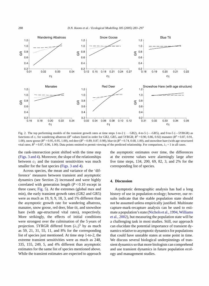
288 D.N. Koons et al. / Ecological Modelling 185 (2005) 283–297
Fig. 2. The top performing models of the transient growth rates at time steps 1-to-2 (· · · GR2), 4-to-5 (- - -GR5), and 0-to-5 (—5YRGR) asfunctions ofc1 for wandering albatross (R2 values listed in order for GR2, GR5, and 5YRGR;R2 = 0.90, 0.86, 0.92) manatee (R2 = 0.87, 0.91,1.00), snow goose (R2 = 0.95, 0.95, 1.00), red deer (R2 = 0.89, 0.87, 0.98), blue tit (R2 = 0.74, 0.68, 1.00), and snowshoe hare (with age-structuredvital rates;R2 = 0.87, 0.96, 1.00). Data points omitted to permit viewing of the predicted relationship. For comparison,λ1 = 1 in all cases.
the rank-intersection point shifted with the time step(Figs. 3 and 4). Moreover, the slope of the relationshipsbetweenc1 and the transient sensitivities was muchsmaller for the fast species (Figs. 3 and 4).
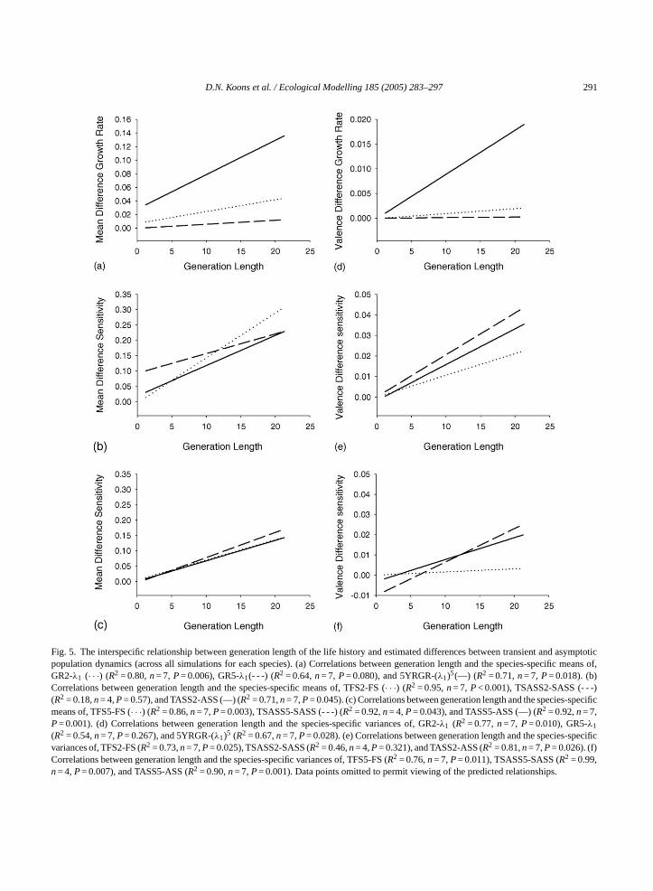
Across species, the mean and variance of the ‘dif-ference’ measures between transient and asymptoticdynamics (see Section2) increased and were highlycorrelated with generation length (P< 0.10 except inthree cases;Fig. 5). At the extremes (global max andmin), the early transient growth rates (GR2 and GR5)were as much as 19, 9, 9, 18, 3, and 1% different thanthe asymptotic growth rate for wandering albatross,manatee, snow goose, red deer, blue tit, and snowshoehare (with age-structured vital rates), respectively.More strikingly, the effects of initial conditionswere strongest over the culmination of the 5 years ofprojection. 5YRGR differed from (λ1)5 by as muchas 59, 21, 31, 55, 11, and 8% for the correspondinglist of species just mentioned. At time step 1-to-2, theextreme transient sensitivities were as much as 248,335, 155, 249, 5, and 4% different than asymptoticestimates for the same list of species mentioned above.While the transient estimates are expected to approach
the asymptotic estimates over time, the differencesat the extreme values were alarmingly large afterfive time steps, 134, 200, 69, 82, 3, and 2% for thecorresponding list of species.
4. Discussion
Asymptotic demographic analysis has had a longhistory of use in population ecology; however, our re-sults indicate that the stable population state shouldnot be assumed unless empirically justified. Multistatecapture-mark-recapture analysis can be used to esti-mate a population’s state (Nichols et al., 1994,Williamset al., 2002), but measuring the population state will bea challenging task in most studies. Still, our approachcan elucidate the potential importance of transient dy-namics relative to asymptotic dynamics for populationsthat could have unstable states at some point in time.We discuss several biological underpinnings of tran-sient dynamics so that more biologists can comprehendand use transient dynamics in future population ecol-ogy and management studies.
D.N. Koons et al. / Ecological Modelling 185 (2005) 283–297 289
Fig. 3. The top performing models of the transient sensitivities [(· · ·) fertility, (- - -) sub-adult survival, and (—) adult survival] at time step 1-to-2as functions ofc1 for wandering albatross (R2 values listed in order for fertility, sub-adult survival, and adult survival;R2 = 0.75, 0.73, 0.74),manatee (R2 = 0.97, 0.97, 0.97), snow goose (R2 = 0.63, 0.86, 0.76), red deer (R2 = 0.71, 0.67, 0.66), blue tit (R2 = 0.93, –, 0.38), and snowshoehare (with age-structured vital rates;R2 = 1.00, –, 0.86). Data points omitted to permit viewing of the predicted relationship. For comparison,(�): asymptotic fertility sensitivity; (�): asymptotic sub-adult survival sensitivity; (�) asymptotic adult survival sensitivity.
4.1. Intraspecific patterns in transient dynamics
Damping ratios (Tuljapurkar, 1986; Law and Edley,1990), asymptotic convergence times (Taylor, 1979;DeAngelis et al., 1980; Hastings and Higgins, 1994),Argand diagrams (Horst, 1977; Rago and Goodyear,1987), examination of oscillations in state vector com-ponents (Tuljapurkar, 1983, 1985) and examinationof unstable equilibrium (Cushing et al., 1998) haveall been used to present transient dynamics. However,these approaches fail to explicitly incorporate measuresof population growth rate, which is one of the unify-ing parameters of ecology and evolution (Sibly et al.,2002).
In our study, we found that transient populationgrowth rates and sensitivities were highly dependenton initial conditions. The initial net reproductive valueusually increased with the signed Keyfitz∆ becauselarge∆s represented population states with proportion-ately more breeding adults than the stable state, andadult age classes frequently had higher reproductivevalue than sub-adult age classes. However, initial netreproductive value decreased with the signed Keyfitz
∆ when vital rates declined with age (e.g., blue tit andred deer;Fig. 1).
Across all of the possible initial population statesfor each species, transient fertility and adult sur-vival sensitivities generally increased withc1, whereasthe transient sub-adult survival sensitivity decreased(Figs. 3 and 4, but see red deer results). This occurredbecause initial population states with lowc1 values gen-erally consisted of more sub-adults or partially senes-cent old individuals than the stable state (seeFig. 1).Individuals must survive to maturity before they cancontribute young to the population, which explains whyearly transient growth rates are generally most sensi-tive to sub-adult survival for initial population stateswith low c1 values. Initial population states with highc1 values largely consisted of individuals that were ator near their peak reproductive value (Fig. 1); thus, thecontinued survival and fertility output of prime-agedadults contributed most to transient population growthrates under these conditions.
The initial net reproductive value (c1) is anomnibus measure that can be used to predict thetransient dynamics (e.g., GR, TSij ) across initial state
290 D.N. Koons et al. / Ecological Modelling 185 (2005) 283–297
Fig. 4. The top performing models of the transient sensitivities [(· · ·) fertility, (- - -) sub-adult survival, and (—) adult survival] at time step 4-to-5as functions ofc1 for wandering albatross (R2 values listed in order for fertility, sub-adult survival, and adult survival;R2 = 0.88, 0.86, 0.86),manatee (R2 = 1.00, 1.00, 1.00), snow goose (R2 = 0.64, 0.87, 0.72), red deer (R2 = 0.93, 0.64, 0.62), blue tit (R2 = 0.97, –, 0.55), and snowshoehare (with age-structured vital rates;R2 = 1.00, –, 0.96). Data points omitted to permit viewing of the predicted relationship. For comparison,(�): asymptotic fertility sensitivity, (�): asymptotic sub-adult survival sensitivity, (�) asymptotic adult survival sensitivity.
conditions, through time, and to examine shifts in therank-order of vital rate contributions to transient GR(seeFigs. 3 and 4). Thus, the net reproductive valueof a population can help explain many properties oftransient dynamics (Templeton, 1980) and it will beimportant to study the ecological forces that affectc1.
4.2. Interspecific patterns in transient dynamics
Tuljapurkar (1985)found that damping ratios andperiods of oscillation in the population state vectorincreased with generation length. In 15 of our 18interspecific comparisons, we found that either themean or variance of the estimated ‘differences’ be-tween transient and asymptotic dynamics increasedwith generation length as well. Furthermore, slopesof the abovementioned intraspecific relationshipswere steepest among slow and medium-slow species(Figs. 2–4).
Population dynamics in fast species were resilient todepartures from the stable state; however, slow species
experienced early transient dynamics that were vari-able across the possible initial-state conditions, verydifferent than asymptotic dynamics, and the dynamicschanged slowly over time as they slowly converged tothe asymptotic stable state. Moreover, unstable pop-ulation states sometimes produced net decreases ornet increases in population size, a phenomenon knownas population momentum (Keyfitz, 1971; Lande andOrzack, 1988; Koons et al., unpublished data).
Compared to fast species, slow species mature lateand live long lives, increasing the chances for high vari-ability in survival rates and reproductive investmentacross the age classes. These life history characteristicslead to high disparity in reproductive value across ageclasses (see rv:rv,Appendix A). Long generation lengthwill increase the time required for transient dynamics tochange (Tuljapurkar, 1985), and disparate reproductivevalues could lead to large changes in net reproductivefollowing changes in population state. Collectively, webelieve these factors make the dynamics of slow speciesmore responsive to changes in population state.
D.N. Koons et al. / Ecological Modelling 185 (2005) 283–297 291
Fig. 5. The interspecific relationship between generation length of the life history and estimated differences between transient and asymptoticpopulation dynamics (across all simulations for each species). (a) Correlations between generation length and the species-specific means of,GR2-λ1 (· · ·) (R2 = 0.80,n= 7, P= 0.006), GR5-λ1(- - -) (R2 = 0.64,n= 7, P= 0.080), and 5YRGR-(λ1)5(—) (R2 = 0.71,n= 7, P= 0.018). (b)Correlations between generation length and the species-specific means of, TFS2-FS (· · ·) (R2 = 0.95,n= 7, P< 0.001), TSASS2-SASS (- - -)(R2 = 0.18,n= 4,P= 0.57), and TASS2-ASS (—) (R2 = 0.71,n= 7,P= 0.045). (c) Correlations between generation length and the species-specificmeans of, TFS5-FS (· · ·) (R2 = 0.86,n= 7,P= 0.003), TSASS5-SASS (- - -) (R2 = 0.92,n= 4,P= 0.043), and TASS5-ASS (—) (R2 = 0.92,n= 7,P= 0.001). (d) Correlations between generation length and the species-specific variances of, GR2-λ1 (R2 = 0.77,n= 7, P= 0.010), GR5-λ1
(R2 = 0.54,n= 7,P= 0.267), and 5YRGR-(λ1)5 (R2 = 0.67,n= 7,P= 0.028). (e) Correlations between generation length and the species-specificvariances of, TFS2-FS (R2 = 0.73,n= 7,P= 0.025), TSASS2-SASS (R2 = 0.46,n= 4,P= 0.321), and TASS2-ASS (R2 = 0.81,n= 7,P= 0.026). (f)Correlations between generation length and the species-specific variances of, TFS5-FS (R2 = 0.76,n= 7,P= 0.011), TSASS5-SASS (R2 = 0.99,n= 4,P= 0.007), and TASS5-ASS (R2 = 0.90,n= 7,P= 0.001). Data points omitted to permit viewing of the predicted relationships.
292 D.N. Koons et al. / Ecological Modelling 185 (2005) 283–297
4.3. Ecological implications
Transient population analysis can reveal the pos-sible effects of initial age or stage structure (Fox andGurevitch, 2000; this study), colonization (Caswell andWerner, 1978), life history (DeAngelis et al., 1980; thisstudy), harvest, and especially pulse perturbations tothe environment (e.g., catastrophic mortality) on pop-ulation dynamics. Of immediate concern, our resultsindicate thatλ1 can be a biased estimate of short-term population growth rate when population stateis unstable (e.g., 335% difference between transientand asymptotic estimates), especially among slow andmedium-slow species.
Popular methods for managing and conserving pop-ulations include release of captive-reared animals intothe wild, relocation of wild individuals (e.g.,Starling,1991; Wolf et al., 1996; Ostermann et al., 2001), andstate-specific harvest management (Larkin, 1977; Holtand Talbot, 1978). All of these methods will perturbpopulation state and produce transient dynamics. At-tempts to identify the best animal propagation or har-vest program with asymptotic projection models couldlead to incorrect conclusions (Merrill et al., 2003)and even mismanagement of populations. Long ago,MacArthur (1960)showed that management programsthat favor individuals with high reproductive value willlead to large net reproductive values, which in turncause high population growth rates and abundance.Programs that favor individuals with low reproductivev or-i nyi im-i ics.U man-a opu-l con-s -termp antt tud-i inga thef
., oila ter-r lo-g enicc
al., 1983; Brockwell, 1985; Lande, 1993; Mangel andTier, 1993, 1994). However, the impact of catastro-phes on population dynamics cannot be elucidatedwith asymptotic methods alone because catastrophescould severely perturb population state. We have shownthat this can drastically alter the short-term populationdynamics, and Koons et al. (unpublished data) haveshown that it can significantly affect long-term pop-ulation size. When catastrophes have the potential toperturb population state, we suggest that risk assess-ments, such as population viability analyses (Gilpinand Soule, 1986) and population recovery analyses,pay closer attention to transient dynamics and the ef-fects of population state on extinction or recovery timesand probabilities.
4.4. Caveats
The degree to which asymptotic dynamics are a poorproxy to actual dynamics depends on the populationstate, time, and life history. Like many transient analy-ses, our results are unique to the time scale and modelsunder examination. Because the number of uniqueeigenvalues and eigenvectors can change with matrixdimension, the chosen matrix dimension may influencetransient dynamics. Yet, we found that expandingsmall-dimension matrices (e.g., 3-by-3, etc.) into alarge-dimension matrix (29-by-29) resulted in transientgrowth rates that were identical to four decimal places.Matrix dimension did affect the net reproductive valuea sta-b sw eta ittler ssaryt cesi k as icalf atedd ent.L ies,a ins f thed er-a ndee ella tiallya
alue will produce opposite results. Moreover, favng few individuals of high reproductive value or mandividuals of low reproductive value can result in slar net reproductive values and transient dynamsing our approach, we suggest that resourcegers place a strong emphasis on estimation of p
ation state and reproductive value to examine theequences of their management actions on shortopulation dynamics, which are often more relev
o agency goals than long-term dynamics. Such ses will help reduce uncertainty in decision-maknd the likelihood of deleterious management in
uture.Furthermore, anthropogenic catastrophes (e.g
nd toxin spills, nuclear disasters, mining, war, bioorism) are common in today’s world and many bioists try to understand the impacts of anthropogatastrophes on population dynamics (Brockwell et
nd the time required to converge to the asymptoticle state (seeCaswell, 2001:97), however differenceere≤0.005 and≤0.05 years, respectively (Koonsl. unpublished data). Thus, in this study we saw leason to use matrices that were larger than neceo incorporate the published age-specific differenn vital rates. Furthermore, we purposefully tooimplistic approach to elucidate some of the biologactors causing transient population growth and relynamics in an otherwise deterministic environmong-term population size, growth rate, sensitivitnd extinction probability can be approximatedtochastic environments for any population state iegree of environmental variability is small to modte (Tuljapurkar, 1982; Lande and Orzack, 1988; Lat al., 2003). In the real world, the vital rates, as ws age, stage, or size structure, may vary substancross time and space (e.g.,Clutton-Brock and
D.N. Koons et al. / Ecological Modelling 185 (2005) 283–297 293
Coulson, 2002). Questions concerning transientdynamics in highly stochastic and periodicallycatastrophic environments have not been examined,and offer an arena for much needed research in thefuture.
Acknowledgements
We thank H. Caswell for his comments on ear-lier renditions of our mathematical solutions and G.Fox, C. Pfister, A. Grant, F.S. Dobson, and two anony-mous reviewers for helpful comments on this work.We particularly appreciate the support of D.V. Derk-sen and Lyman K. Thorsteinson of USGS, BiologicalResources Division. The USGS, Biological ResourcesDivision, Alaska Biological Science Center funded thisresearch.
Wandering albatross Manatee Snow goose Red deer Blue tit Snowshoe harea Snowshoe hareb
K 0.97 0.95 0.91 0.94 0.88 0.91 0.92T 21.29 14.34 5.63 7.73 1.52 1.24 1.23r 2.
A α Fi
12 183 α 0.0 184 0.15 0.26 0.27 0.28 0.29 0.21 0.21 0.21 0.21 0.1...
Appendix A
Age-specific values of average age-at-maturity (de-noted byα), fertility (F), and survival rates (P) inthe standardized matrices for wandering albatross(Weimerskirch, 1992; Weimerskirch et al., 1997), man-atee (Eberhardt and O’Shea, 1995), snow goose (Cookeet al., 1995; Cooch et al., 2001), red deer (Benton et al.,1995, Albon et al., 2000), blue tit (Dhondt, 1989a, b),and snowshoe hare (Meslow and Keith, 1968). Also,standardizing constants (K), which were multiplied tothe original life-cycle matrices parameterized with vi-tal rates attained from the literature, generation lengths(T, the time required for the population to increase bya factor ofR0 [the net reproductive rate]), and dispar-ity of reproductive value across age classes (rv:rv, theratio of the highest age-specific reproductive value tothe lowest).
v:rv 3.10 1.32 1.77
gec α Fi Pi α Fi Pi α Fi Pi
0.81 0.91 0.740.81 0.91 α 0.17 0.740.81 0.91 0.33 0.740.81 α 0.12 0.91 0.40 0.740.94 0.12 0.91 0.46 0.740.940.940.940.94
0 α 0.22 0.941 0.22 0.942 0.22 0.943 0.22 0.94
0.22 0.94
92 1.15 1.09 1.00
Pi α Fi Pi α Fi Pi α Fi Pi
0.85 α 0.65 0.34 α 0.81 0.18 α 0.82 0.180.91 0.69 0.34 0.85 0.18 0.82 0.
8 0.90 0.69 0.34 0.89 0.18 0.82 0.9 0.90 0.59 0.341 0.90 0.59 0.341 0.901 0.901 0.861 0.861 0.861 0.861 0.866 0.65
294 D.N. Koons et al. / Ecological Modelling 185 (2005) 283–297
(Continued)
Agec α Fi Pi α Fi Pi α Fi Pi α Fi Pi α Fi Pi α Fi Pi α Fi Pi
19 0.22 0.9420 0.20 0.94... 0.20 0.9428 0.20 0.9429 0.20 0.90
†All numerical values in the table are rounded to the nearest 10−2 decimal place. In the projection analysis we used values with precision to the10−6 decimal place;††the division of the values in the table byK yields the original vital-rate values.
a Snowshoe hare life-cycle with age-structured vital rates.b Snowshoe hare life-cycle without age-structured vital rates.c Pseudo age class.
Appendix B
Traditionally, populations have been modeled withmatrix equations of the form
nt = Atn0 (B.1)
where nt and n0 are vectors describing the popu-lation state (i.e., age, stage, or size distribution) attimes t and 0, respectively, andA is an n×n (de-terministic) matrix whose entries are denoted byaij(we denote matrices and vectors in bold type withupper-case and lower-case notation, respectively). Al-ternatively, Eq.(B.1) can be decomposed and ex-pressed with the eigenvalues and eigenvectors of theAmatrix,
nt =∑
i
ciλtiwi (B.2)
where thewi ’s are the right eigenvectors ofA, theλi ’sare the associated eigenvalues, and theci ’s are depen-dent on initial conditions and the complex conjugates ofthe left eigenvectors ofA (Caswell, 2001). The dom-inant right eigenvector (w1) and the dominant scalar(c1) describe the asymptotic stable state and net re-productive value of the initial population (Templeton,1980), respectively. The biological definitions of thesub-dominant eigenvectors and scalars are less clear(Caswell, 2001). Still, Eq. (B.2) can provide a deeperunderstanding of the dynamics ofn , but some may findi
.( s
(2000) pioneering work by deriving a complexbut elegant solution to the sensitivity of ‘transientpopulation growth rate’ to infinitely small changesin a vital rate. His method allows one to calculatethe sensitivity of the average transient growth ratefor specific age or stage classes, or for the entirepopulation. If one does not need detailed informationabout class-specific dynamics, we derive a simplersolution to the sensitivity of transient populationgrowth rate of the entire population to infinitely smallchanges in a vital rate that begins with Eq.(B.1) ratherthan Eq.(B.2).
As described in the text, the population growth rateof a population in any state (not assuming the stablestate) can be defined according to Eq.(2). Becausent inEq.(2) is derived from theA matrix and the initial statevector, our definition of growth rate is quantitativelyequivalent toYearsley’s (2004)calculation that uses theweighted average of the eigenvalue spectrum belongingto theA matrix (the individual state vector componentsat timet−1 in our Eq.(2) operate as the weights). Forcomparative purposes, population growth rates for thek-th element of the population state vector can simplybe calculated by deleting the summation symbols inour Eq. (2). Furthermore, to estimate the populationgrowth rate over any time stepm, the denominator ofEq.(2) can be changed tont−m, k.
Nevertheless, our goal was to find a simple analyt-ical solution to the sensitivity of the transient GR for
es
e
t
t difficult to work with.For these reasons,Yearsley (2004)begins with Eq
B.2) to projectnt and appendsFox and Gurevitch’
the entire population to infinitesimally small changin a vital-rate (TSij , Eq.(3)). To do this we begin withEq. (B.1) to projectnt. We note thatA0 is defined asthe identity matrix. We denotedeas the vector whos

D.N. Koons et al. / Ecological Modelling 185 (2005) 283–297 295
components are all equal to 1 and∆ij as then×nmatrix whose entry in thei-th row andj-th column is 1 and 0everywhere else. We make special note that fort= 1, 2,. . .
∂
∂aij
At =t−1∑l=0
Al∆ijAt−l−1 (B.3)
wherel simply operates as a dummy variable. We then use this definition of the partial derivative of theA matrixwith respect to one of its entries to derive the sensitivity of transient growth rate to changes in theA-matrix entries.Thus, fort= 1
∂(∑
knt,k/∑
knt−1,k
)∂aij
= ∂
∂aij
e′An0
e′n0= e′∆ijn0
e′n0(B.4)
and fort= 2, 3,. . .
∂(∑
knt,k/∑
knt−1,k
)∂aij
= ∂
∂aij
e′Atn0
e′At−1n0
= (∂/∂aij)[e′Atn0]e′At−1n0 − e′Atn0(∂/∂aij)[e′At−1n0]
(e′At−1n0)2
=∑t−1
l=0e′Al∆ijAt−l−1n0e′At−1n0 − e′Atn0
∑t−2l=0e
′Al∆ijAt−l−2n0
(e′At−1n0)2
(B.5)
where the last expression can also be written in the form,
∑t−2l=0e
′Al∆ijAt−l−2(An0e′ − n0e′A)At−1n0 + e′At−1∆ijn0e′At−1n0
(e′At−1n0)2
(B.6)
Therefore, given Eqs.(B.5) and (B.6),
TSij =
e′∆ijn0
e′n0for t = 1
∑t−2l=0e
′Al∆ijAt−l−2(An0e′ − n0e′A)At−1n0 + e′At−1∆ijn0e′At−1n0
(e′At−1n0)2
for t = 2, 3, . . .
(B.7)
References
Akaike, H., 1973. Information theory and an extension of the max-imum likelihood principle. In: Petran, B.N., Csaki, F. (Eds.),International Symposium on Information Theory, second ed.Akademiai Kiado, Budapest.
Albon, S.D., Coulson, T.N., Brown, D., Guinness, F.E., Pemberton,J.M., Clutton-Brock, T.H., 2000. Temporal changes in key fac-tors and key age groups influencing the population dynamics offemale red deer. J. Anim. Ecol. 69, 1099–1110.
Benton, T.G., Grant, A., Clutton-Brock, T.H., 1995. Does environ-mental stochasticity matter? Analysis of red deer life-histories inRum. Evolut. Ecol. 9, 559–574.
Benton, T.G., Grant, A., 1999. Elasticity analysis as an important toolin evolutionary and population ecology. Trends Ecol. Evolut. 14,467–471.
Bierzychudek, P., 1999. Looking backwards: assessing the projec-tions of a transition matrix model. Ecol. Appl. 9, 1278–1287.
Brockwell, P.J., Gani, J.M., Resnick, S.I., 1983. Catastrophe pro-cesses with continuous state space. Aust. N. Z. J. Stat. 25,208–226.
Brockwell, P.J., 1985. The extinction time of a birth, death and catas-trophe process and of a related diffusion model. Adv. Appl. Prob.17, 42–52.
Burnham, K.P., Anderson, D.R., 1998. Model Selection and In-ference: A Practical Information-Theoretic Approach. Springer,New York.

296 D.N. Koons et al. / Ecological Modelling 185 (2005) 283–297
Carroll, R.J., Ruppert, D., 1988. Transformation and Weighting inRegression. Chapman and Hall, New York.
Caswell, H., Werner, P.A., 1978. Transient behavior and life historyanalysis of teasel (Dipsacus sylvestrisHuds). Ecology 59, 53–66.
Caswell, H., 1978. A general formula for the sensitivity of populationgrowth rate to changes in life history parameters. Theor. Popul.Biol. 14, 215–230.
Caswell, H., 2001. Matrix Population Models: Construction, Anal-ysis and Interpretation, second ed.. Sinauer Associates, MA.
Charnov, E.L., 1993. Life History Invariants: Some Explorations ofSymmetry in Evolutionary Ecology. Oxford University Press,Oxford.
Clutton-Brock, T.H., Coulson, T., 2002. Comparative ungulate dy-namics: the devil is in the detail. Phil. Trans. R. Soc. Lond. B357, 1285–1298.
Coale, A.J., 1972. The Growth and Structure of Human Populations:a Mathematical Approach. Princeton University Press, Princeton.
Cohen, J.E., 1976. Ergodicity of age structure in populations withMarkovian vital rates. I: countable states. J. Am. Stat. Assoc. 71,335–339.
Cohen, J.E., 1977a. Ergodicity of age structure in populations withMarkovian vital rates. II: general states. Adv. Appl. Prob. 9,18–37.
Cohen, J.E., 1977b. Ergodicity of age structure in populations withMarkovian vital rates. III: finite-state moments and growth rate;an illustration. Adv. Appl. Prob. 9, 462–475.
Cohen, J.E., 1979. Ergodic theorems in demography. Bull. Am. Math.Soc. 1, 275–295.
Cooch, E.G., Rockwell, R.F., Brault, S., 2001. Retrospective anal-ysis of demographic responses to environmental change: anexample in the lesser snow goose. Ecol. Monogr. 71, 377–400.
Cooke, F., Rockwell, R.F., Lank, D.B., 1995. The snow geese of LaPerouse Bay. Oxford University Press, Oxford.
C toticiol.
C 998.opu-
D D.S.,sity-del.
D ro-
D tion
E life-ck-theton,
F ls for
Fujiwara, M., Caswell, H., 2001. Demography of the endangeredNorth Atlantic right whale. Nature 414, 537–541.
Gaillard, J.M., Pontier, D., Allaine, D., Lebreton, J.D., Trouvilliez,J., Clobert, J., 1989. An analysis of demographic tactics in birdsand mammals. Oikos 56, 59–76.
Gilpin, M.E., Soule, M.E., 1986. Minimum viable populations: pro-cesses of species extinction. In: Soule, M.E. (Ed.), ConservationBiololgy: The Science of Scarcity and Diversity. Sinauer Asso-ciates, MA.
Goodman, L.A., 1968. An elementary approach to the populationprojection-matrix, to the population reproductive value, and torelated topics in the mathematical theory of population growth.Demography 5, 382–409.
Hastings, A., Higgins, K., 1994. Persistence of transients in spatiallystructured ecological models. Science 263, 1133–1136.
Hastings, A., 2001. Transient dynamics and persistence of ecologicalsystems. Ecol. Lett. 4, 215–220.
Hastings, A., 2004. Transients: the key to long-term ecological un-derstanding. Trends Ecol. Evolut. 19, 39–45.
Heppell, S.S., Pfister, C., de Kroon, H., 2000a. Elasticity analysis inpopulation biology: methods and applications. Ecology 81, 606.
Heppell, S.S., Caswell, H., Crowder, L.B., 2000b. Life histories andelasticity patterns: perturbation analysis for species with minimaldemographic data. Ecology 81, 654–665.
Holt, S.J., Talbot, L.M., 1978. New principles for the conservationof wild living resources. Wildl. Monogr., 59.
Horst, T.J., 1977. Use of the Leslie matrix for assessing environmen-tal impact with an example for a fish population. Trans. Am. Fish.Soc. 106, 253–257.
Horvitz, C.C., Schemske, D.W., Caswell, H., 1997. The “impor-tance” of life history stages to population growth: prospectiveand retrospective analyses. In: Tuljapurkar, S., Caswell, H. (Eds.),Structured Population Models in Marine, Terrestrial and Fresh-water Systems. Chapman and Hall, New York.
Keyfitz, N., 1968. Introduction of the Mathematics of Population.
K og-
K op-
L ge-Natl.
L phic. Am.
L n Dy-ess,
L ined
L with0.
L eton
M alue145.
ull, P., Vogt, A., 1973. Mathematical analysis of the asympbehavior of the Leslie population matrix model. Bull. Math. B35, 645–661.
ushing, J.M., Dennis, B., Desharnais, R.A., Costantino, R.F., 1Moving toward an unstable equilibrium: saddle nodes in plation systems. J. Anim. Ecol. 67, 298–306.
eAngelis, D.L., Svoboda, L.J., Christensen, S.W., Vaughn,1980. Stability and return times of Leslie matrices with dendependent survival: applications to fish populations. Ecol. Mo8, 149–163.
hondt, A.A., 1989a. Blue tit. In: Newton, I. (Ed.), Lifetime Repduction in Birds. Academic Press, London.
hondt, A.A., 1989b. The effect of old age on the reproducof great titsParus majorand blue titsP. caeruleus. Ibis 131,268–280.
berhardt, L.L., O’Shea, T.J., 1995. Integration of manateehistory data and population modeling. In: O’Shea, T.J., Aerman, B.B., Percival, H.F. (Eds.), Population Biology ofFlorida Manatee. U.S. Department of the Interior, WashingDC.
ox, G.A., Gurevitch, J., 2000. Population numbers count: toonear-term demographic analysis. Am. Nat. 156, 242–256.
Addison-Wesley, MA.eyfitz, N., 1971. On the momentum of population growth. Dem
raphy 8, 71–80.eyfitz, N., 1972. Population waves. In: Greville, T.N.E. (Ed.), P
ulation Dynamics. Academic Press, New York.ande, R., Orzack, S.H., 1988. Extinction dynamics of a
structured populations in a fluctuating environment. Proc.Acad. Sci. U.S.A. 85, 7418–7421.
ande, R., 1993. Risks of population extinction from demograand environmental stochasticity and random catastrophesNat. 142, 911–927.
ande, R., Engen, S., Sæther, B.-E., 2003. Stochastic Populationamics in Ecology and Conservation. Oxford University PrOxford.
arkin, P.A., 1977. An epitaph for the concept of maximum sustayield. Trans. Am. Fish. Soc. 106, 1–11.
aw, R., Edley, M.T., 1990. Transient dynamics of populationsage- and size-dependent vital rates. Ecology 71, 1863–187
opez, A., 1961. Problems in Stable Population Theory. PrincUniversity Press, Princeton.
acArthur, R.H., 1960. On the relation between reproductive vand optimal predation. Proc. Natl. Acad. Sci. U.S.A. 46, 143–

D.N. Koons et al. / Ecological Modelling 185 (2005) 283–297 297
Mangel, M., Tier, C., 1993. Dynamics of metapopulations with de-mographic stochasticity and environmental catastrophes. Theor.Popul. Biol. 44, 1–31.
Mangel, M., Tier, C., 1994. Four facts every conservation biologistshould know about persistence. Ecology 75, 607–614.
Merrill, J.A., Cooch, E.G., Curtis, P.D., 2003. Time to reduction: fac-tors influencing management efficacy in sterilizing overabundantwhite-tailed deer. J. Wildl. Manage. 67, 267–279.
Mertz, D.B., 1971. Life history phenomena in increasing and de-creasing populations. In: Patil, G.P., Pielou, E.C., Waters, W.E.(Eds.), Statistical ecology. II. Sampling and modeling biologicalpopulations and population dynamics. Pennsylvania State Uni-versity Press, University Park.
Meslow, E.C., Keith, L.B., 1968. Demographic parameters of a snow-shoe hare population. J. Wildl. Manage. 32, 812–834.
Neter, J., Kutner, M.H., Nachsteim, C.J., Wasserman, W., 1996. Ap-plied Linear Statistical Models. Irwin, Chicago.
Nichols, J.D., Hines, J.E., Pollock, K.H., Hinz, R.L., Link, W.A.,1994. Estimating breeding proportions and testing hypothesesabout costs of reproduction with capture-recapture data. Ecology75, 2052–2065.
Oli, M.K., Zinner, B., 2001. Partial life-cycle analysis: a model forpre-breeding census data. Oikos 93, 376–387.
Ostermann, S.D., Deforge, J.R., Edge, W.D., 2001. Captive breedingand reintroduction evaluation criteria: a case study of peninsularbighorn sheep. Conserv. Biol. 15, 749–760.
Rago, P.J., Goodyear, C.P., 1987. Recruitment mechanisms of stripedbass and Atlantic salmon: comparative liabilities of alternativelife histories. Am. Fish. Soc. Symp. 1, 402–416.
Rockwell, R.F., Cooch, E.G., Brault, S., 1997. High goose popu-lations: causes, impacts and implications. In: Batt, B.J. (Ed.),Arctic Ecosystems in Peril: Report of the Arctic Goose HabitatWorking. Arctic Goose Joint Venture Special Publication, U.S.Fish and Wildlife Service, Washington, DC.
Rousseeuw, P.J., Leroy, A.M., 1987. Robust Regression and Outlier
S con-ate.
S o ainingoc.
Starling, A.E., 1991. Workshop summary: captive breeding and re-lease. Ornis Scand. 22, 255–257.
Taylor, F., 1979. Convergence to the stable age distribution in popu-lations of insects. Am. Nat. 113, 511–530.
Templeton, A.R., 1980. The evolution of life histories underpleiotropic constraints and r-selection. Theor. Popul. Biol. 18,279–289.
Trussell, T.J., 1977. Determinants of roots of Lotka’s equation. Math.Biosci. 36, 213–227.
Tuljapurkar, S.D., 1982. Population dynamics in variable environ-ments. II. Correlated environments, sensitivity analysis and dy-namics. Theor. Popul. Biol. 21, 114–140.
Tuljapurkar, S.D., 1983. Transient dynamics of yeast populations.Math. Biosci. 64, 157–167.
Tuljapurkar, S.D., 1984. Demography in stochastic environments.I. Exact distributions of age structure. J. Math. Biol. 19, 335–350.
Tuljapurkar, S.D., 1985. Population dynamics in variable environ-ments. VI. Cyclical environments. Theor. Popul. Biol. 28, 1–17.
Tuljapurkar, S.D., 1986. Demography in stochastic environments. II.Growth and convergence rates. J. Math. Biol. 24, 569–581.
Tuljapurkar, S.D., 1990. Population Dynamics in Variable Environ-ments. Springer-Verlag, New York.
van Groenendael, J., de Kroon, H., Caswell, H., 1988. Projectionmatrices in population biology. Trends Ecol. Evolut. 3, 264–269.
Weimerskirch, H., 1992. Reproductive effort in long-lived birds: age-specific patterns of condition, reproduction and survival in thewandering albatross. Oikos 64, 464–473.
Weimerskirch, H., Brothers, N., Jouventin, P., 1997. Population dy-namics of wandering albatrossDiomedea exulansand Amster-dam albatrossD. amsterdamensisin the Indian ocean and theirrelationships with long-line fisheries: conservation implications.Biol. Conserv. 79, 257–270.
Williams, B.K., Nichols, J.D., Conroy, M.J., 2002. Analysis andSan
W ndurvey
Y -termdel.
Detection. Wiley and Sons, New York.æther, B.-E., Bakke, O., 2000. Avian life history variation and
tribution of demographic traits to the population growth rEcology 81, 642–653.
ibly, R.M., Hone, J., Clutton-Brock, T.H., 2002. Introduction tdiscussion meeting issue ‘population growth rate: determfactors and role in population regulation’. Phil. Trans. R. SLond. B 357, 1149–1151.
Management of Animal Populations. Academic Press,Diego.
olf, C.M., Griffith, B., Reed, C., Temple, S.A., 1996. Avian amammalian translocations: update and reanalysis of 1987 sdata. Conserv. Biol. 10, 1142–1154.
earsley, J.M., 2004. Transient population dynamics and shortsensitivity analysis of matrix population models. Ecol. Mo177, 245–258.