Embed Size (px)
Citation preview
1
Transient Modelling and Simulation of Gas Turbine Secondary Air System
Theoklis Nikolaidis¹*, Haonan Wang¹, Panagiotis Laskaridis¹
¹ Centre of Propulsion Engineering, Cranfield University, Cranfield, UK
* Corresponding author – [email protected]
Abstract
The behaviour of the jet engine during transient operation and specifically its secondary air
system (SAS) is the point of this work. This paper presents a methodological approach to
develop a fast, one-dimensional transient platform for preliminary analysis of the flow
behaviour in gas turbine engines secondary air system. For this purpose, different elements
of the system including rotating chamber, pipe, turbine blade cooling, orifice, and labyrinth
seal are modelled in a modular form. The validity of the developed models for each component
is checked against experimental/publicly available data. Then, using a flow network simulation
approach, the secondary air system of a two-spool turbofan engine is modelled and simulated
in transient mode. The coupling effect between volume packing and swirl are considered in
the simulation, under two pre-defined scenarios for step and scheduled boundary condition
variations. In the step-change scenario, the boundary conditions are changed instantly to
represent the flow behaviour of the SAS under extreme operating conditions (i.e. shaft
fracture, flameout, etc.). In the scheduled scenario, the boundary conditions vary linearly with
time to represent the performance of the SAS under normal operating conditions (i.e.
acceleration and deceleration). The key findings include the fact that, under normal engine
operation, the flow in the SAS varies smoothly and converges much faster than the primary
flow by around one magnitude. Thus, it is reasonable to use steady-state SAS model to
simulate SAS flow behaviour under these conditions. However, under extreme conditions (e.g.
flameout), which could induce an abrupt change in the primary airflow properties (pressure,
temperature), reverse airflow or choking conditions in SAS may be observed. This could result
in a malfunction of the SAS, inducing further damages to the engine.
Keywords: Secondary air system, transient modelling and simulation, gas turbine engines,
extreme operating conditions effects.
2
Nomenclature
Abbreviations
COT Combustor Outlet Temperature
FSP Front Sump Pressurization
HPT High-Pressure Turbine
HPC High-Pressure Compressor
OD Off Design
OPR Overall Pressure Ratio
PR Pressure Ratio
RR Rolls-Royce
SAS Secondary Air System
TET Turbine Entry Temperature
Symbol� Nozzle Area �� Cross Section Area of The Cooling Passage �� External Blade Surface Area ����� Bi Number of The Thermal Barrier Coating ���� Bi Number of The Blade Wall ��total ����� − ��� − ��
1 − �� � ����� Clearance �� Discharge Coefficient �� Constant Volume Specific Heat �� Flow Coefficient,
����� Pipe/Nozzle Diameter � Angular Flux
�� Friction Factor ℎ� Gas Heat Transfer Coefficient �� ��� ���,���,� � ������
K�� Carry-Over Factor
K� V�/��� Pipe/ Nozzle Length �� Disk Moment �� Shroud Moment ��� Mass in Cavity � Mass Flow Rate
n� Labyrinth Seal Teeth Number
P Pressure � Teeth Distance ���� Heat Input Due to Disc Windage And Convection �� Reynold’s Number � Gas Constant � Radius
r� Inner Radius
r� Outer Radius �� Reynold’s Number � Shroud Width ��� Stanton Number
T Temperature � Time/ Teeth Thickness � Velocity ��� Cavity Volume γ Specific Heat Ratio
3
� Pipe Surface Absolute Roughness �� Convection Cooling Effectiveness �� Cooling Efficiency �� Cooling Efficiency of Blade with Film Cooling � Through Flow Parameter ��� Conductivity Coefficient of Blade Metal ���� Conductivity Coefficient of Thermal Barrier Coating � Viscosity � Gas Density ∅ Coolant Mass Flow Ratio � Angular Velocity Δ Difference Δ��� Thermal Barrier Coating Thickness
�� Blade Thickness
Subscripts
1 Upstream
2 Downstream� Total � Blade � Coolant � disc � Film � Gas �� Inlet ��� Outlet � Static ��� Thermal Barrier Coating � Axial Direction � Tangential Direction
Superscripts � Average
1. Introduction
The secondary air system (SAS) of a gas turbine engine ensures that the engine can operate
safely and perform efficiently. The air is extracted from the main gas path (therefore, it does
not contribute to the thrust or power generation directly) and it is diverted to serve different
engine systems (e.g. turbine blade cooling, oil sump pressurization, bearing control loading,
etc.). It is well known that SAS operation affects the engine performance. Therefore, it is of
primary importance to model the effects of SAS during the preliminary design for engines.
Different flow elements, which have been developed as independent modules, can be used to
build typical secondary airflow branches in a gas turbine engine, such as the turbine blade
cooling air, the oil sump pressurization air, the disc cavity ventilation air, the axial bearing load
control, etc. However, from the performance perspective, there are always efficiency losses
associated with SAS. Typically, for a modern turbofan engine, an increase of 11K in turbine
entry temperature is required to compensate 1% rise in secondary air mass flow to maintain
4
the same level of thrust [1]. Thus, SAS should be designed meticulously to achieve its
functions with the minimum amount of bleeding air [2].
The investigation on SAS analysis has been in wide interests for a long time. The mainstream
is implementing appropriate flow network to represent the SAS and to analyse the flow
behaviour in the network. In 1992, Kutz and Speer [3] firstly introduced the flow network
method for gas turbine SAS modelling. The authors have considered heat transfer along the
flow path, choking in the pipe, two-phase flow, reverse flow and several pipes connecting in
series. Although the results obtained from this method was satisfactory, its complexity appears
as a huge obstacle for preliminary analysis as fast-run codes are needed in an iterative
procedure of the preliminary design. In 2009, Alexiou et al [4] developed a model with fewer
flow conditions considered (i.e. two-phase flow) in an object-oriented environment that allows
the creation of different configurations in a simple and flexible manner. Che et al. [5] proposed
a unified component method to model the SAS and the main gas path together to save the
effort for establishing an interface between them. Besides the traditional deterministic models,
Brack et al [6] put forward a probabilistic model to account for the uncertainty in the SAS due
to geometric variations from engine to engine and varied engine operational conditions. In
addition to the 1-D network, there are many research studies on integrating 1-D/ 2-D/ 3-D
models to account for thermomechanical effects on performance as well as irregular
geometries [7-9].
The above-mentioned studies focused on steady-state performance simulations. However,
the behaviour of SAS during transient conditions should be investigated, as several
phenomena may take place, which cannot be captured during steady-state simulations.
Simulating the SAS at transient conditions may detect and prevent short excess in axial
bearing loading and helps to understand the system’s dynamic characteristics under extreme
conditions (e.g. when flameout, disc burst, or shaft fracture) [10].
Recently, several methods have been published on the modelling of SAS transient
performance. Gallar [11] and Calcagni [12] have developed a SAS modelling platform, which
has been successfully validated with SPAN, a Rolls-Royce (RR) in-house program for
performing SAS calculation. The dynamic properties of the pipe have been modelled
comprehensively in their work. However, the rotating effects of elements were not considered.
In 2010, May and Chew proposed an initial method to account for the rotating effects in
transient simulation [13]. They later improved the initial methods to simulate the transient
performance of a de-swirl nozzle by considering more details of the swirl structure in the
rotating chamber [14]. The swirl structure is utilized to assess the radial pressure distribution
in the chamber and for a better thermal model. However, they focused on a standalone flow
5
element of the chamber and did not extend their investigation to flow network simulation.
Moreover, the effects on different operating conditions on the behaviour of SAS have not been
considered yet.
In this paper, the coupling effect between volume packing and swirl is considered as a step
further in SAS transient simulation. Besides, other elements were also developed to support
a full-branch analysis of the flow network. At the same time, the platform is constrained to one-
dimensional for a faster calculation speed. Therefore, the main contribution of this work is the
development of a fast, one-dimensional transient platform for preliminary analysis of the flow
behaviour in the gas turbine engine SAS. The tool is utilized to simulate the transient
performance under both normal and extreme conditions considering the coupling effect
between volume packing and swirl in a full flow network.
For this purpose, section two describes the methodology and validation of the platform
components. The different elements of the SAS system (i.e. rotating chamber, pipe, and
turbine cooling passages, orifice, and labyrinth seal) are presented in this section. The
developed models are validated against available experimental data. In section three, the flow
network simulation for the different SAS branches (the front sump pressurization branch, high-
pressure turbine rotor cooling branch, and cavity ventilation branch) is demonstrated. In
section four, the analysis and discussion of the results are presented, followed by the
conclusion remarks in section five.
2. Methodology and Validation of the Platform In this paper, the one-dimensional flow network method is used for the modelling of transient
performance of the SAS. The flow elements in the transient modelling platform are categorised
into volumes and flow path elements, which are connected to form the system network. The
volumetric effects and gas inertia are considered for the volumes while the flow path elements
just serve as inlet and outlet of the volumes.
The physical SAS transient process will take place once there is a deviation from equilibrium
engine operating points, i.e. due to transient in the primary airflow system. The air mass flow
and pressure change will affect the SAS inlet conditions and a new energy and mass flow
balance should be achieved. Based on the physical process, the transient performance is
modelled as follow: at each time step, the mass flow rate is firstly calculated from pressure
imbalance at each flow element, and then the air temperature is calculated according to
different heat transfer processes taking place at each flow element.
A typical gas turbine engine SAS can be modelled by using a library of five elements: a rotating
chamber, a pipe and turbine cooling passages, which are classified as volumes; and an orifice,
a labyrinth seal, which are treated as a flow path. After establishing the network from the flow
6
elements, parameters specifying the element characteristics, boundary conditions, initial
pressure and temperature within the chamber should be provided to initialize the calculation.
The chamber’s pressure, temperature and the mass flow rate on each branch will be
calculated to satisfy the boundary conditions. The mathematical model and the corresponding
assumptions made for each element are explained in the following sections.
2.1. Element modelling The mathematical modelling of different components of the SAS system will be presented in
this section.
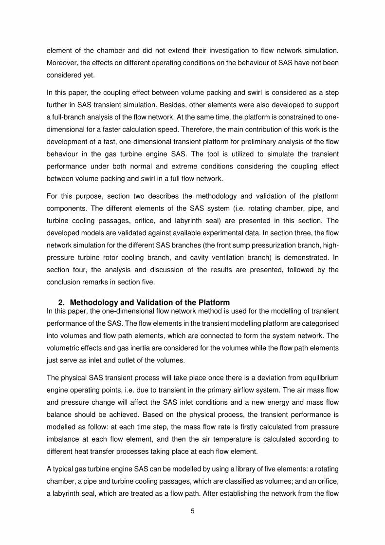
2.1.1 Modelling of the rotating chamber A schematic of a rotating chamber is shown in Figure 1. The inlet flow could be injected radially
(Figure 1 (a)) or axially (Figure 1 (b)). The direction could have an impact on the vortex
structure in the chamber. It is assumed that the chamber is in constant size, rectangular shape
and the gas properties keep uniform in the axial direction.
(a) (b)
Figure 1: Schematic of a rotating chamber [21]:
(a) with radially inward flow; (b) with axially inward flow
The mathematical modelling has been based on the work from May et al in [13-14]. However,
in [13-14], the convection heat transfer with the surroundings was not considered. Its inclusion
in this model is based on the work of Alexiou et al [4].
It is assumed that the tangential velocity profile satisfies:
V� = K� ∗ r�(1)
where V� presents tangential velocity; K� is a constant; r is the radius and n is vortex index,
indicating the vortex behaviour in the chamber. Equation (1) shows that the tangential velocity
varies exponentially along the radius. When n equals to 1, the tangential velocity of the flow
in the chamber maintains a forced vortex profile; when n equals to -1, a free vortex structure
Ω Ω

7
will be observed in the flow. For axial inflow from any radius, the vortex structure is assumed
to be forced vortex, which means vortex index n should be 1. For radial inflow, it is assumed
that the vortex index could be determined by the through-flow parameter λ [14]:
� =�����.� (2)
where
�� =�� (3)
where �� represents the flow coefficient; μ is the viscosity; � the mass flow rate; ��represents the outer cavity radius and �� is Reynold’s number.
According to [10], the relationship between vortex index n and through-flow parameter λ
could be estimated as:
� = � 1, �� − 0.001 < � < 0.01 −1, �� � < −1 �� � > 0.4
However, when λ is outside of the range (i.e. −1 < � < − 0.001 �� 0.01 < � < 0.4 ), there
is no determinant relationship in this transition area. It may be assumed that it varies
exponentially or linearly [10]. A linear relationship is assumed in this paper for simplicity
(Figure 2).
Figure 2: Vortex index vs. through flow parameter
The rate of chamber average static pressure change can be obtained from the mass
conservation law: ����� =������ ⋅ (��� − ����) +
���� ����� (4)
8
where ��� represents the constant cavity volume, � is the gas constant and �� and �� are
the average chamber static pressure and temperature respectively. It should be noted that, in
this model the swirl structure is used for calculating the disc windage and radial pressure
distribution is not considered for a faster calculation.
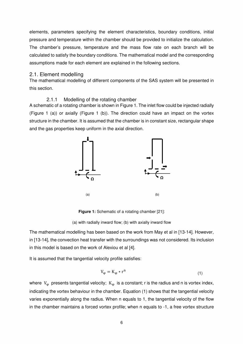
The rate of chamber static temperature change can be calculated from energy conservation
law:
����� =1��� �� ������ + ��� ������,����,�� − ������,�����,��� − ����(��� − ����) + �����
(5)
The kinetic energy variation has been neglected in equation (5), and it is assumed that the
mass flow out of the chamber at average temperature and pressure. ���� in the equation (5)
consists of the work input due to disc windage and convection heat transfer from the disc.
Conduction through the disc wall has not been considered in this model. Determination of
these values can be found in Appendix equations (A-11) to (A-13). The swirl velocity �� can
be obtained from angular momentum conservation law: ��� ����(1� + 3
)(����� − �������� )� =
1
2�� �� �� + � �� − ���� + ���� (6)
where �� and �� represents the inner and outer cavity radius respectively, � is the shroud
width, �� and �� are the disc moment and shroud moment respectively. Their estimation
can be found in the Appendix equations (A-1) to (A-10). � represents the angular flux entering
and exiting the cavity:
���� = �������������(7)��� = �����,����� (8)
2.1.2. Modelling of the pipe A pipe is modelled as a rotating chamber with a large length to volume ratio. In the 1-D pipe
model, due to the small radius of it, the angular momentum effect is not considered. The basic
mass, momentum and energy conservation laws are similar to that of the chamber (equation
(4)-(6)). Darcy–Weisbach’s formula has been selected to model the total pressure loss [25]:
∆P = � ∙ �� ∙ �2
∙ �2� (9)
9
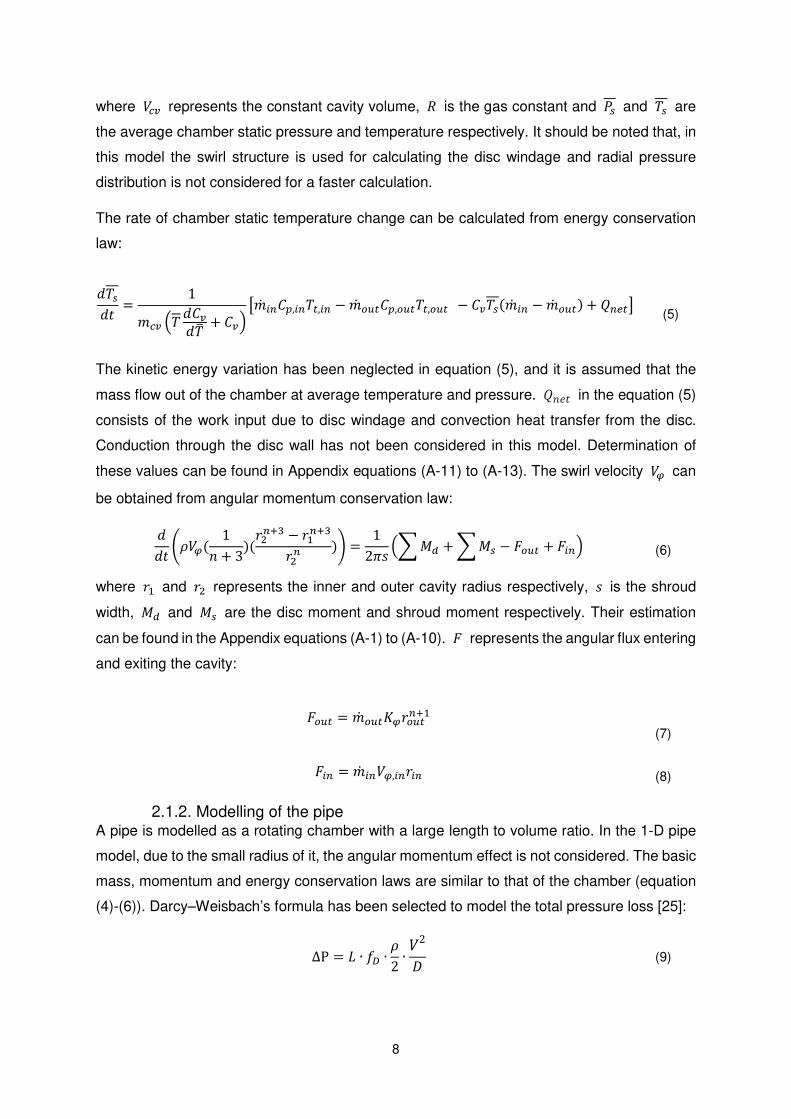
where ∆P represents the total pressure loss; � is the pipe length; � is air density; �represents the flow velocity in the pipe; D is the pipe diameter and �� is the friction factor,
which is determined using Moody’s formula [25]:
�� = 0.0055 �1 + �2 × 10⁴ ∙ �� +106�� �1/3� (10)
where � represents the absolute roughness of pipe surface and �� is the Reynold’s number
of the air.
2.1.3 Modelling of the turbine blade cooling In the turbine blade cooling model, there are two processes: the pumping and heat transfer
process, which are considered separately. Initially, the process in the cooling passage is
assumed adiabatic. Given this, a pipe element is used to model the pumping effect in order to
calculate the coolant mass flow rate, which is available in the cooling passage. The next step
is to enable the heat transfer model and evaluate the blade temperature. In other words, the
blade temperature is calculated based on instant coolant mass flow and combustor outlet
temperature (COT). These two distinct processes do not compromise the accuracy of the
results considerably, as the flow pressure does not influence the heat transfer in the classical
analytical blade cooling model.
The restricting effect through the coolant passage is the same as the pipe analyzed in the
previous section. For the thermal effects, a semi-empirical model is implemented for the
preliminary analysis of the blade cooling effects [15]. The assumptions used for this model are
the uniform bulk gas around blade, uniform external heat transfer coefficients, constant
thermodynamic properties and uniform metal temperature. Some technical empirical data
should be provided to obtain the blade metal temperature, which are shown in Table 1.
Table 1: Empirical technical values input for turbine blade cooling element
Symbol Meaning Definition
����� Bi number of the thermal
barrier coating ����� =
ℎ�Δ����������� Bi number of the blade wall ���� =ℎ�Δ������� Cooling efficiency of blade
with film cooling �� =
�� − ���� − ��,����� Cooling efficiency �� =��,��� − ��,���� − ��,��
10
��� Stanton number ��� =ℎ�
(��/��)��,�Given the coolant mass flow ratio ∅, which can be obtained from the SAS calculation, the
convection cooling effectiveness �� can be solved from the following equation:
∅ =���� =
��1 + ������� �� − ��[1 − ��(1 − ��)]��(1 − ��) (11)
where �� ��total can be calculated as:
�� = ��� ���,���,� � ����� � (12)
��total = ����� − ��� − ��1 − �� � ���� (13)
where the definition ���, ��, �����, ���� can be found in Table 1; ��,� is the specific heat
capacity of the hot gas and ��,� is the specific heat capacity of the coolant; �� is the external
blade surface area which can be estimated as the product of the blade perimeter and the blade
span; and �� is the cross sectional area of the coolant passage.
Given ��, the blade temperature can be obtained from the equation:
�� =�� − ���� − ��,�� (14)
where �� represents the TET and it can be extracted from the main path calculation; ��,��represents the inlet coolant temperature which can be obtained from SAS calculation system.
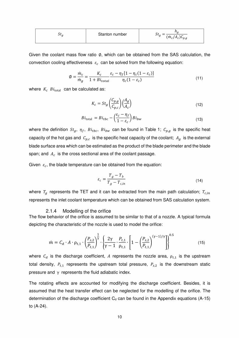
2.1.4 Modelling of the orifice The flow behavior of the orifice is assumed to be similar to that of a nozzle. A typical formula
depicting the characteristic of the nozzle is used to model the orifice:
� = �� ∙ � ∙ ρ�,� ∙ ���,���,���� ∙ � 2γγ − 1∙ ��,�ρ�,� ∙ �1 − ���,���,��(���)/����.�
(15)
where �� is the discharge coefficient, � represents the nozzle area, ρ�,� is the upstream
total density, ��,� represents the upstream total pressure, ��,� is the downstream static
pressure and γ represents the fluid adiabatic index.
The rotating effects are accounted for modifying the discharge coefficient. Besides, it is
assumed that the heat transfer effect can be neglected for the modelling of the orifice. The
determination of the discharge coefficient Cd can be found in the Appendix equations (A-15)
to (A-24).
11
Moreover, flow reversal and choking have been considered in the orifice element in this study.
Given the upstream total pressure and downstream static pressure, the algorithm would check
firstly if the pressure ratio is larger than one. If so, it indicates that the downstream static
pressure is larger than upstream pressure, and the air would flow reversely. The flow function
is:
� = −�� ∙ � ∙ ρ�,� ∙ ���,���,����� ∙ � 2γγ − 1∙ ��,2ρ�,2
∙ �1 − ���,2��,1
�−(γ−1)/γ���.�(16)
And then, the algorithm would check if the pressure ratio is larger than the critical value to
determine whether the orifice is choked. If it’s choked, the pressure ratio used to drive the air
is the critical one:
������ = �1 +� − 1
2��−1�
(17)
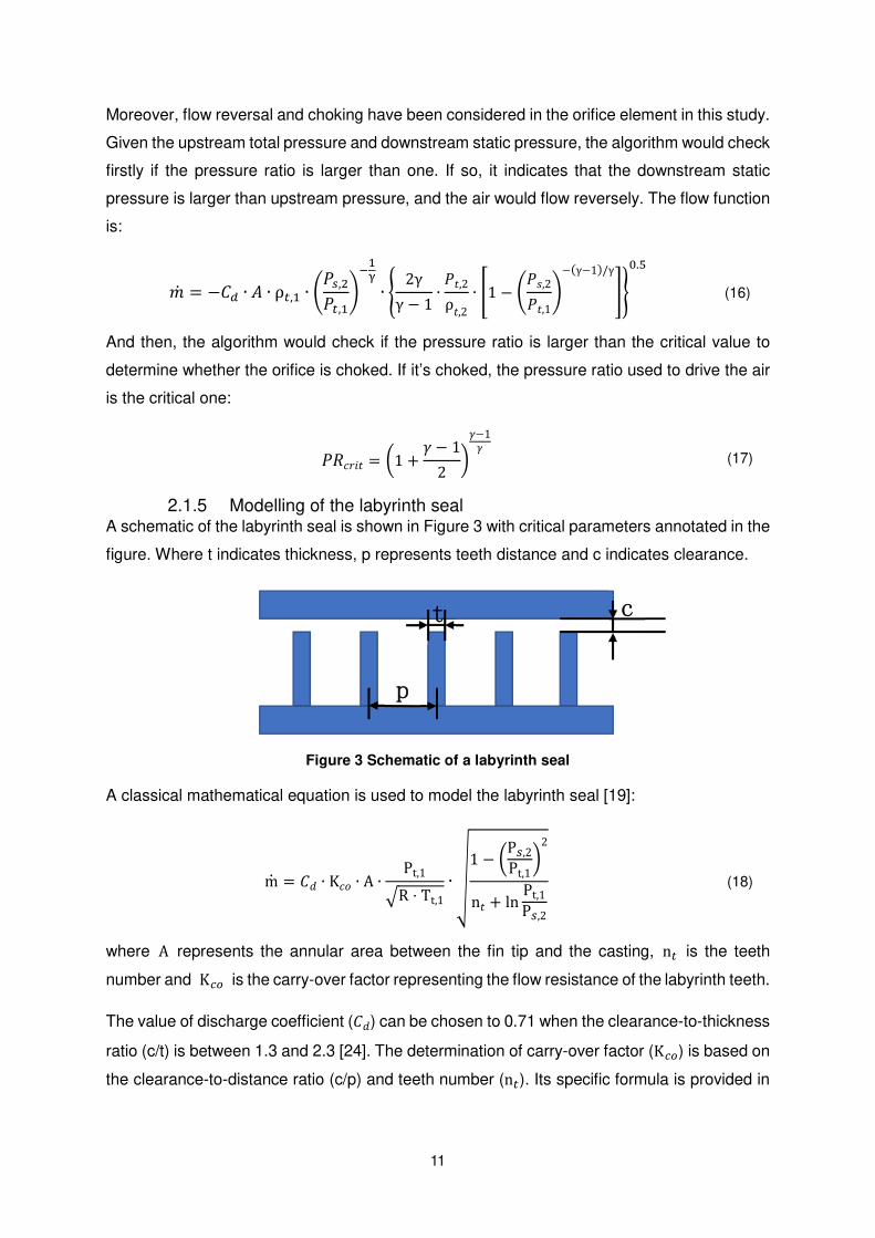
2.1.5 Modelling of the labyrinth seal A schematic of the labyrinth seal is shown in Figure 3 with critical parameters annotated in the
figure. Where t indicates thickness, p represents teeth distance and c indicates clearance.
Figure 3 Schematic of a labyrinth seal
A classical mathematical equation is used to model the labyrinth seal [19]:
m = �� ∙ K�� ∙ A ∙ Pt,1�R ⋅ Tt,1
∙ �1 − �P�,2
Pt,1�2
n� + lnPt,1
P�,2
(18)
where A represents the annular area between the fin tip and the casting, n� is the teeth
number and K�� is the carry-over factor representing the flow resistance of the labyrinth teeth.
The value of discharge coefficient (��) can be chosen to 0.71 when the clearance-to-thickness
ratio (c/t) is between 1.3 and 2.3 [24]. The determination of carry-over factor (K��) is based on
the clearance-to-distance ratio (c/p) and teeth number (n�). Its specific formula is provided in
t c
p

12
the Appendix equation (A-14). The consideration of flow reversal and choking is done in a
similar way to the orifice model described in the previous sub-section.
2.2. Element Validation and Parametric Study In order to confirm the validity of the modelling approach, some elements have been validated
against experimental/publicly available data.
2.2.1 Validation of the rotating chamber The first test is to demonstrate the coupling effect of disc windage moments and vortex
structure for a chamber with radially inward flow. A schematic display of the rotating chamber
is shown in Figure 1 (a). The inner radius of the chamber is 0.1 m and the outer radius is 0.5
m. The hypothetical fluid ( � = 10 ��/�� , � = 10�� �� ∙ � ) is assumed to enter the
chamber from the outer radius at half-disc rim speed. Then, the cumulative moment and
tangential velocity profile along the radius direction is recorded as vortex index (�) changes
from -1 to 1, where K and ��,���� in Appendix equation (A-5) are set to be 1 and 0.002
respectively.
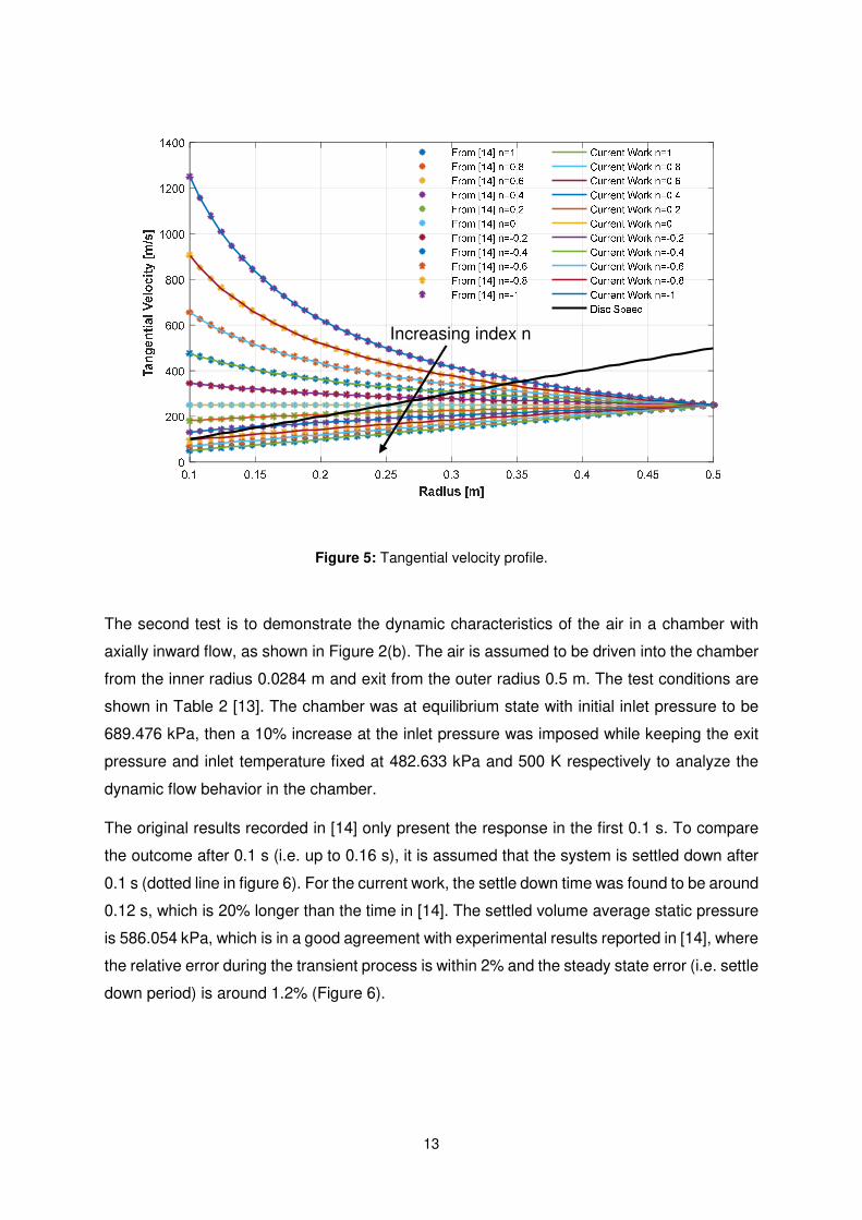
The results showed that both parameters (cumulative moment M and tangential velocity profile ��) align perfectly with those published in [14] (Figure 4 and Figure 5 respectively).
Figure 4: Cumulative moment profile.
Increasing index n
13
Figure 5: Tangential velocity profile.
The second test is to demonstrate the dynamic characteristics of the air in a chamber with
axially inward flow, as shown in Figure 2(b). The air is assumed to be driven into the chamber
from the inner radius 0.0284 m and exit from the outer radius 0.5 m. The test conditions are
shown in Table 2 [13]. The chamber was at equilibrium state with initial inlet pressure to be
689.476 kPa, then a 10% increase at the inlet pressure was imposed while keeping the exit
pressure and inlet temperature fixed at 482.633 kPa and 500 K respectively to analyze the
dynamic flow behavior in the chamber.
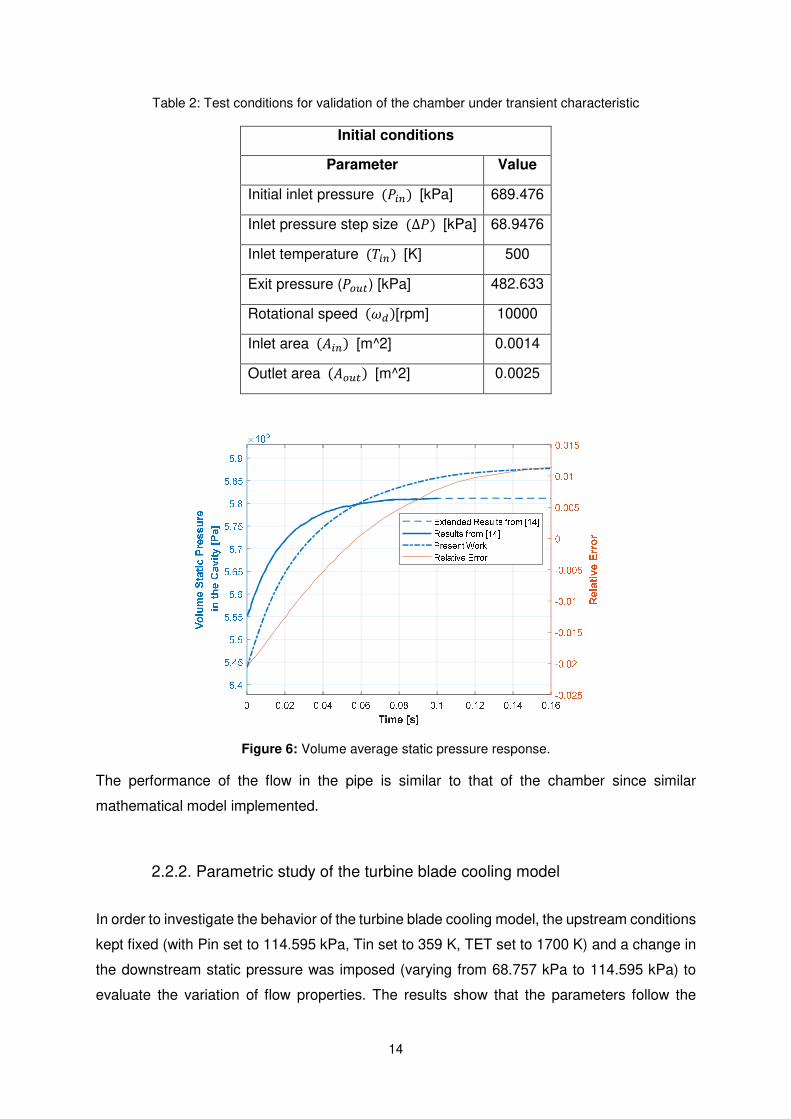
The original results recorded in [14] only present the response in the first 0.1 s. To compare
the outcome after 0.1 s (i.e. up to 0.16 s), it is assumed that the system is settled down after
0.1 s (dotted line in figure 6). For the current work, the settle down time was found to be around
0.12 s, which is 20% longer than the time in [14]. The settled volume average static pressure
is 586.054 kPa, which is in a good agreement with experimental results reported in [14], where
the relative error during the transient process is within 2% and the steady state error (i.e. settle
down period) is around 1.2% (Figure 6).
Increasing index n
14
Table 2: Test conditions for validation of the chamber under transient characteristic
Initial conditions
Parameter Value
Initial inlet pressure (���) [kPa] 689.476
Inlet pressure step size (∆�) [kPa] 68.9476
Inlet temperature (���) [K] 500
Exit pressure (����) [kPa] 482.633
Rotational speed (��)[rpm] 10000
Inlet area (���) [m^2] 0.0014
Outlet area (����) [m^2] 0.0025
Figure 6: Volume average static pressure response.
The performance of the flow in the pipe is similar to that of the chamber since similar
mathematical model implemented.
2.2.2. Parametric study of the turbine blade cooling model
In order to investigate the behavior of the turbine blade cooling model, the upstream conditions
kept fixed (with Pin set to 114.595 kPa, Tin set to 359 K, TET set to 1700 K) and a change in
the downstream static pressure was imposed (varying from 68.757 kPa to 114.595 kPa) to
evaluate the variation of flow properties. The results show that the parameters follow the
15
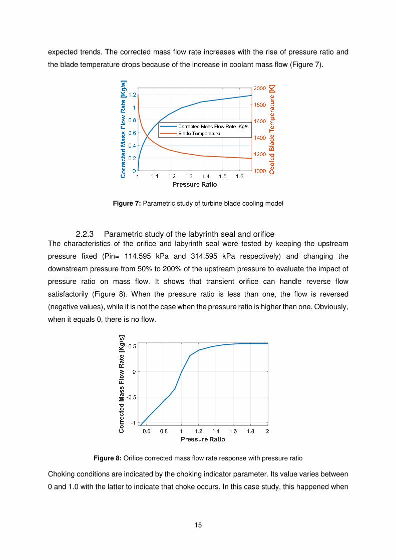
expected trends. The corrected mass flow rate increases with the rise of pressure ratio and
the blade temperature drops because of the increase in coolant mass flow (Figure 7).
Figure 7: Parametric study of turbine blade cooling model
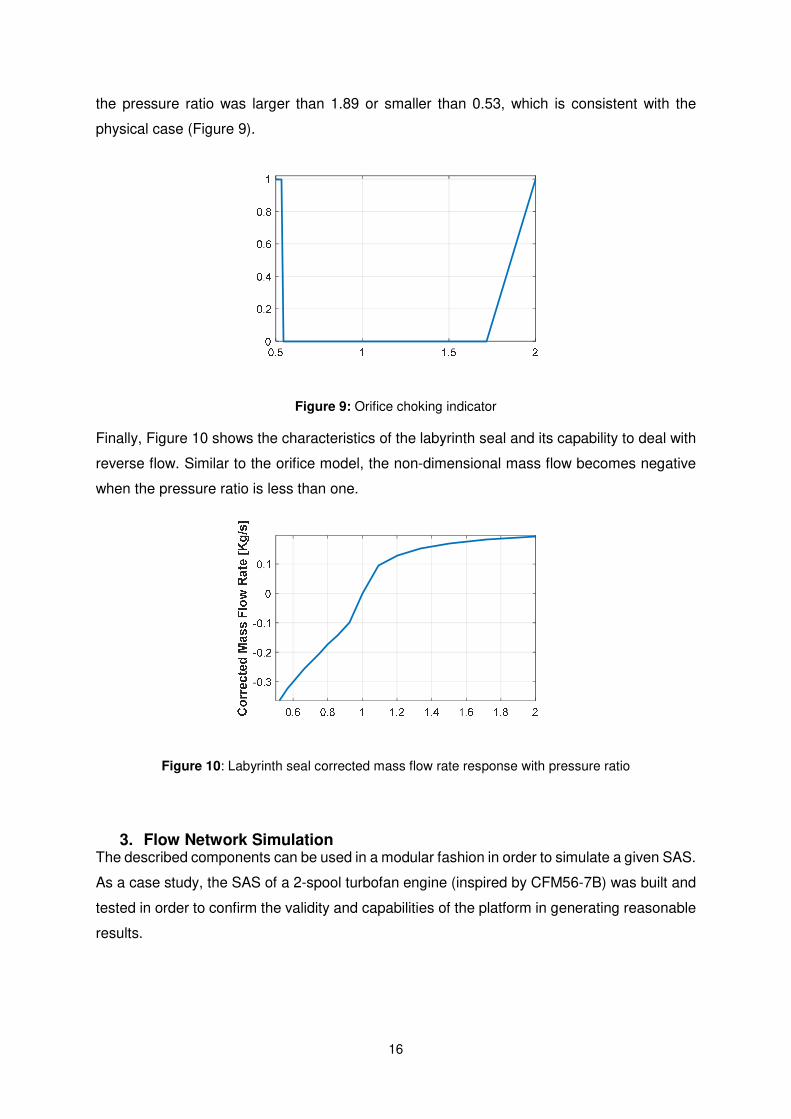
2.2.3 Parametric study of the labyrinth seal and orifice The characteristics of the orifice and labyrinth seal were tested by keeping the upstream
pressure fixed (Pin= 114.595 kPa and 314.595 kPa respectively) and changing the
downstream pressure from 50% to 200% of the upstream pressure to evaluate the impact of
pressure ratio on mass flow. It shows that transient orifice can handle reverse flow
satisfactorily (Figure 8). When the pressure ratio is less than one, the flow is reversed
(negative values), while it is not the case when the pressure ratio is higher than one. Obviously,
when it equals 0, there is no flow.
Figure 8: Orifice corrected mass flow rate response with pressure ratio
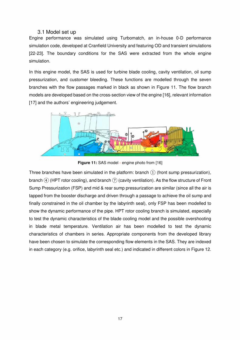
Choking conditions are indicated by the choking indicator parameter. Its value varies between
0 and 1.0 with the latter to indicate that choke occurs. In this case study, this happened when
16
the pressure ratio was larger than 1.89 or smaller than 0.53, which is consistent with the
physical case (Figure 9).
Figure 9: Orifice choking indicator
Finally, Figure 10 shows the characteristics of the labyrinth seal and its capability to deal with
reverse flow. Similar to the orifice model, the non-dimensional mass flow becomes negative
when the pressure ratio is less than one.
Figure 10: Labyrinth seal corrected mass flow rate response with pressure ratio
3. Flow Network Simulation The described components can be used in a modular fashion in order to simulate a given SAS.
As a case study, the SAS of a 2-spool turbofan engine (inspired by CFM56-7B) was built and
tested in order to confirm the validity and capabilities of the platform in generating reasonable
results.
17
3.1 Model set up Engine performance was simulated using Turbomatch, an in-house 0-D performance
simulation code, developed at Cranfield University and featuring OD and transient simulations
[22-23]. The boundary conditions for the SAS were extracted from the whole engine
simulation.
In this engine model, the SAS is used for turbine blade cooling, cavity ventilation, oil sump
pressurization, and customer bleeding. These functions are modelled through the seven
branches with the flow passages marked in black as shown in Figure 11. The flow branch
models are developed based on the cross-section view of the engine [16], relevant information
[17] and the authors’ engineering judgement.
Figure 11: SAS model - engine photo from [16]
Three branches have been simulated in the platform: branch ① (front sump pressurization),
branch ④ (HPT rotor cooling), and branch ⑦ (cavity ventilation). As the flow structure of Front
Sump Pressurization (FSP) and mid & rear sump pressurization are similar (since all the air is
tapped from the booster discharge and driven through a passage to achieve the oil sump and
finally constrained in the oil chamber by the labyrinth seal), only FSP has been modelled to
show the dynamic performance of the pipe. HPT rotor cooling branch is simulated, especially
to test the dynamic characteristics of the blade cooling model and the possible overshooting
in blade metal temperature. Ventilation air has been modelled to test the dynamic
characteristics of chambers in series. Appropriate components from the developed library
have been chosen to simulate the corresponding flow elements in the SAS. They are indexed
in each category (e.g. orifice, labyrinth seal etc.) and indicated in different colors in Figure 12.

18
Figure 12: Model set up scheme – engine photo from [16]
A diagram representing the SAS integrating with the primary airflow is also shown in Figure
13.
Figure 13: SAS flow network diagram
3.2 Test definition Two transient cases are defined to test the behaviour of the designed system at both normal
and extreme working conditions.
The first case (I) simulates the flow behaviour under extreme working conditions (e.g.
flameout) by introducing a step-change in the P & T boundary conditions.
The second case (II) simulates the flow behaviour under normal engine operation (e.g.
acceleration and deceleration) by introducing a scheduled, linear and smooth variation
of the boundary conditions.
3.2.1 Case I: Extreme operating condition This case simulates the flow when there is a step-change in the boundary conditions. In the
beginning, the SAS is in equilibrium state at the maximum operating condition, and then, the
• Boundary conditions
• Orifice
• Labyrinth seal
• Blade cooling
• Rotating chamber
• Pipe

19
boundary conditions suddenly change to their minimum values. The two conditions are
distinguished by the fuel flow to represent flameout situation, as shown in Table 3, and the
corresponding boundary conditions for SAS are shown in Table 4.
Table 3: Test engine operation condition range
Test Index Altitude (m) Mach Delta T (K) Fuel flow (kg/s)
Initial 0 0 15 1.2285
Final 0 0 15 0.41813
Table 4: step change of the boundary conditions
Branch
Inlet Outlet
Pressure
(P) [kPa]
Temperature
(T) [K]
Pressure
(P) [kPa]
Temperature
(T) [K]
Initial ①⑦ 310.0545 434 149.961 827 ④ 3120.81 876 2999.22 1680
Final ①⑦ 176.3055 362 112.4708 659 ④ 1459.08 691 1398.285 1240
3.2.2 Case II: Normal operating condition The scheduled transient test simulates the expected operation of the SAS when there is a
smooth change in the boundary conditions. The initial and final values of the engine operating
conditions are the same as case one, shown in tables 3 and 4. The variation of the boundary
conditions represents the transient performance of the primary air system during deceleration.
20
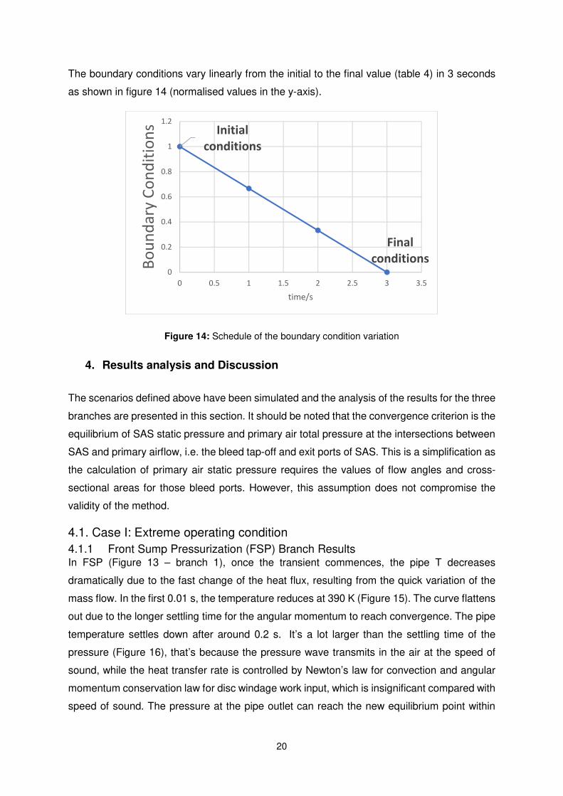
The boundary conditions vary linearly from the initial to the final value (table 4) in 3 seconds
as shown in figure 14 (normalised values in the y-axis).
Figure 14: Schedule of the boundary condition variation
4. Results analysis and Discussion
The scenarios defined above have been simulated and the analysis of the results for the three
branches are presented in this section. It should be noted that the convergence criterion is the
equilibrium of SAS static pressure and primary air total pressure at the intersections between
SAS and primary airflow, i.e. the bleed tap-off and exit ports of SAS. This is a simplification as
the calculation of primary air static pressure requires the values of flow angles and cross-
sectional areas for those bleed ports. However, this assumption does not compromise the
validity of the method.
4.1. Case I: Extreme operating condition
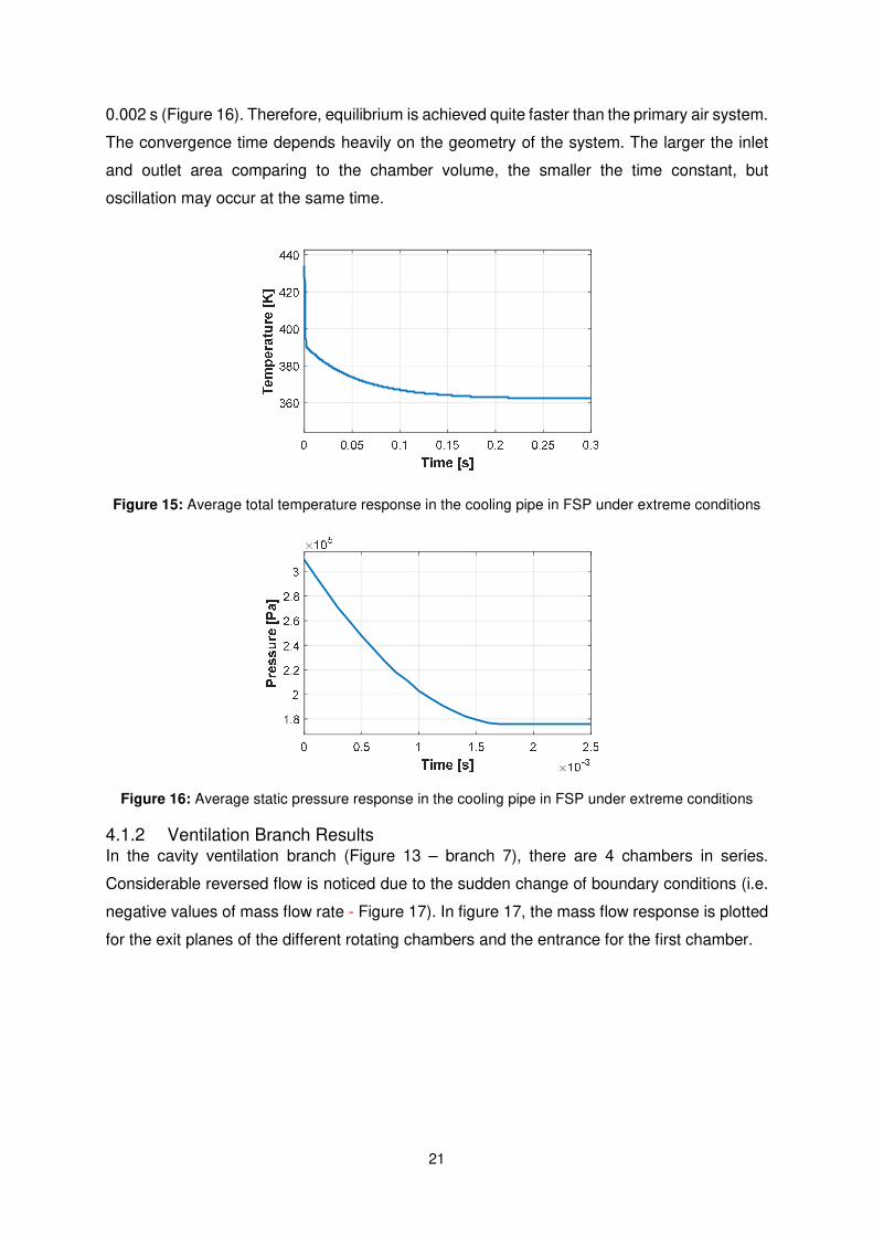
4.1.1 Front Sump Pressurization (FSP) Branch Results In FSP (Figure 13 – branch 1), once the transient commences, the pipe T decreases
dramatically due to the fast change of the heat flux, resulting from the quick variation of the
mass flow. In the first 0.01 s, the temperature reduces at 390 K (Figure 15). The curve flattens
out due to the longer settling time for the angular momentum to reach convergence. The pipe
temperature settles down after around 0.2 s. It’s a lot larger than the settling time of the
pressure (Figure 16), that’s because the pressure wave transmits in the air at the speed of
sound, while the heat transfer rate is controlled by Newton’s law for convection and angular
momentum conservation law for disc windage work input, which is insignificant compared with
speed of sound. The pressure at the pipe outlet can reach the new equilibrium point within
Initial
conditions
Final
conditions
0
0.2
0.4
0.6
0.8
1
1.2
0 0.5 1 1.5 2 2.5 3 3.5
Bo
un
da
ry C
on
dit
ion
s
time/s
21
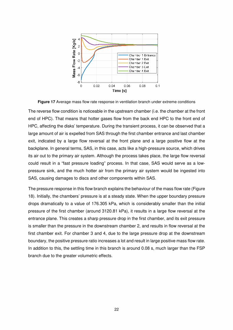
0.002 s (Figure 16). Therefore, equilibrium is achieved quite faster than the primary air system.
The convergence time depends heavily on the geometry of the system. The larger the inlet
and outlet area comparing to the chamber volume, the smaller the time constant, but
oscillation may occur at the same time.
Figure 15: Average total temperature response in the cooling pipe in FSP under extreme conditions
Figure 16: Average static pressure response in the cooling pipe in FSP under extreme conditions
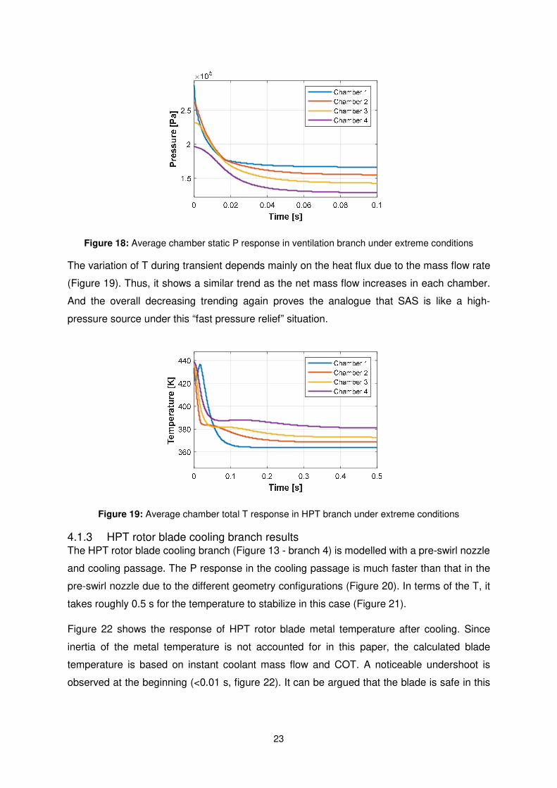
4.1.2 Ventilation Branch Results In the cavity ventilation branch (Figure 13 – branch 7), there are 4 chambers in series.
Considerable reversed flow is noticed due to the sudden change of boundary conditions (i.e.
negative values of mass flow rate - Figure 17). In figure 17, the mass flow response is plotted
for the exit planes of the different rotating chambers and the entrance for the first chamber.
22
Figure 17 Average mass flow rate response in ventilation branch under extreme conditions
The reverse flow condition is noticeable in the upstream chamber (i.e. the chamber at the front
end of HPC). That means that hotter gases flow from the back end HPC to the front end of
HPC, affecting the disks’ temperature. During the transient process, it can be observed that a
large amount of air is expelled from SAS through the first chamber entrance and last chamber
exit, indicated by a large flow reversal at the front plane and a large positive flow at the
backplane. In general terms, SAS, in this case, acts like a high-pressure source, which drives
its air out to the primary air system. Although the process takes place, the large flow reversal
could result in a “fast pressure loading” process. In that case, SAS would serve as a low-
pressure sink, and the much hotter air from the primary air system would be ingested into
SAS, causing damages to discs and other components within SAS.
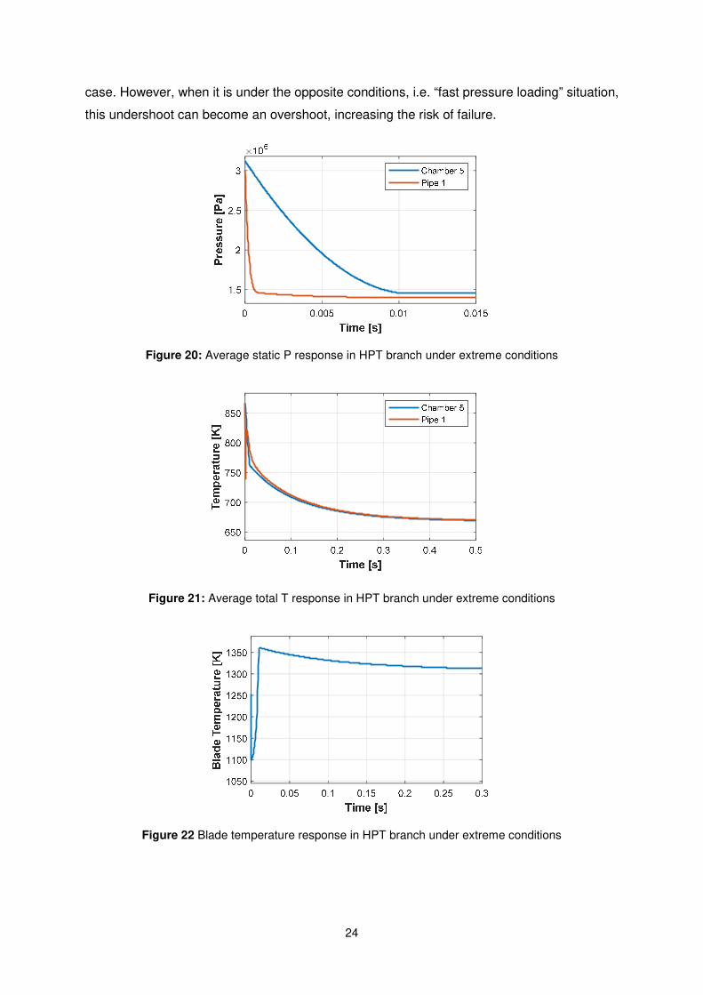
The pressure response in this flow branch explains the behaviour of the mass flow rate (Figure
18). Initially, the chambers’ pressure is at a steady state. When the upper boundary pressure
drops dramatically to a value of 176.305 kPa, which is considerably smaller than the initial
pressure of the first chamber (around 3120.81 kPa), it results in a large flow reversal at the
entrance plane. This creates a sharp pressure drop in the first chamber, and its exit pressure
is smaller than the pressure in the downstream chamber 2, and results in flow reversal at the
first chamber exit. For chamber 3 and 4, due to the large pressure drop at the downstream
boundary, the positive pressure ratio increases a lot and result in large positive mass flow rate.
In addition to this, the settling time in this branch is around 0.08 s, much larger than the FSP
branch due to the greater volumetric effects.
23
Figure 18: Average chamber static P response in ventilation branch under extreme conditions
The variation of T during transient depends mainly on the heat flux due to the mass flow rate
(Figure 19). Thus, it shows a similar trend as the net mass flow increases in each chamber.
And the overall decreasing trending again proves the analogue that SAS is like a high-
pressure source under this “fast pressure relief” situation.
Figure 19: Average chamber total T response in HPT branch under extreme conditions
4.1.3 HPT rotor blade cooling branch results The HPT rotor blade cooling branch (Figure 13 - branch 4) is modelled with a pre-swirl nozzle
and cooling passage. The P response in the cooling passage is much faster than that in the
pre-swirl nozzle due to the different geometry configurations (Figure 20). In terms of the T, it
takes roughly 0.5 s for the temperature to stabilize in this case (Figure 21).
Figure 22 shows the response of HPT rotor blade metal temperature after cooling. Since
inertia of the metal temperature is not accounted for in this paper, the calculated blade
temperature is based on instant coolant mass flow and COT. A noticeable undershoot is
observed at the beginning (<0.01 s, figure 22). It can be argued that the blade is safe in this
24
case. However, when it is under the opposite conditions, i.e. “fast pressure loading” situation,
this undershoot can become an overshoot, increasing the risk of failure.
Figure 20: Average static P response in HPT branch under extreme conditions
Figure 21: Average total T response in HPT branch under extreme conditions
Figure 22 Blade temperature response in HPT branch under extreme conditions
25
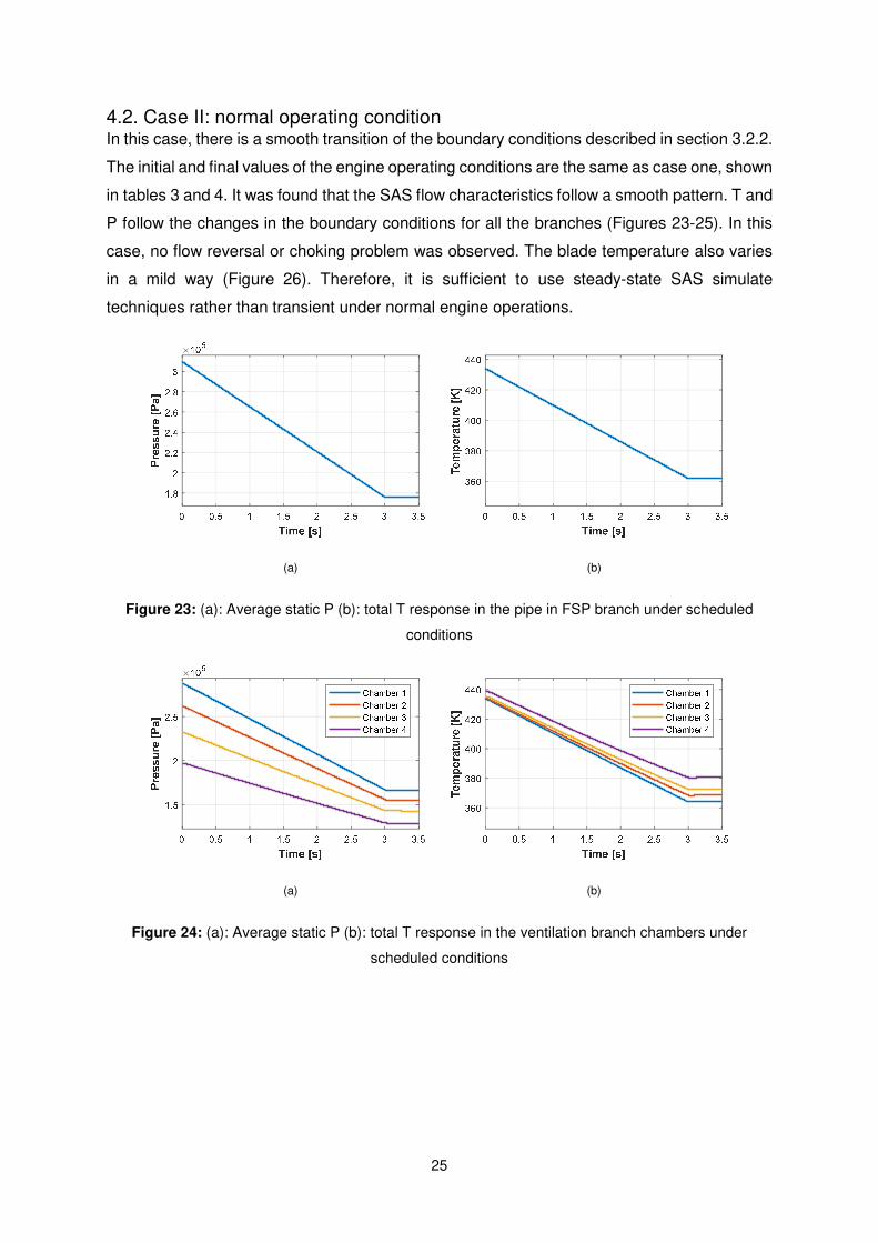
4.2. Case II: normal operating condition In this case, there is a smooth transition of the boundary conditions described in section 3.2.2.
The initial and final values of the engine operating conditions are the same as case one, shown
in tables 3 and 4. It was found that the SAS flow characteristics follow a smooth pattern. T and
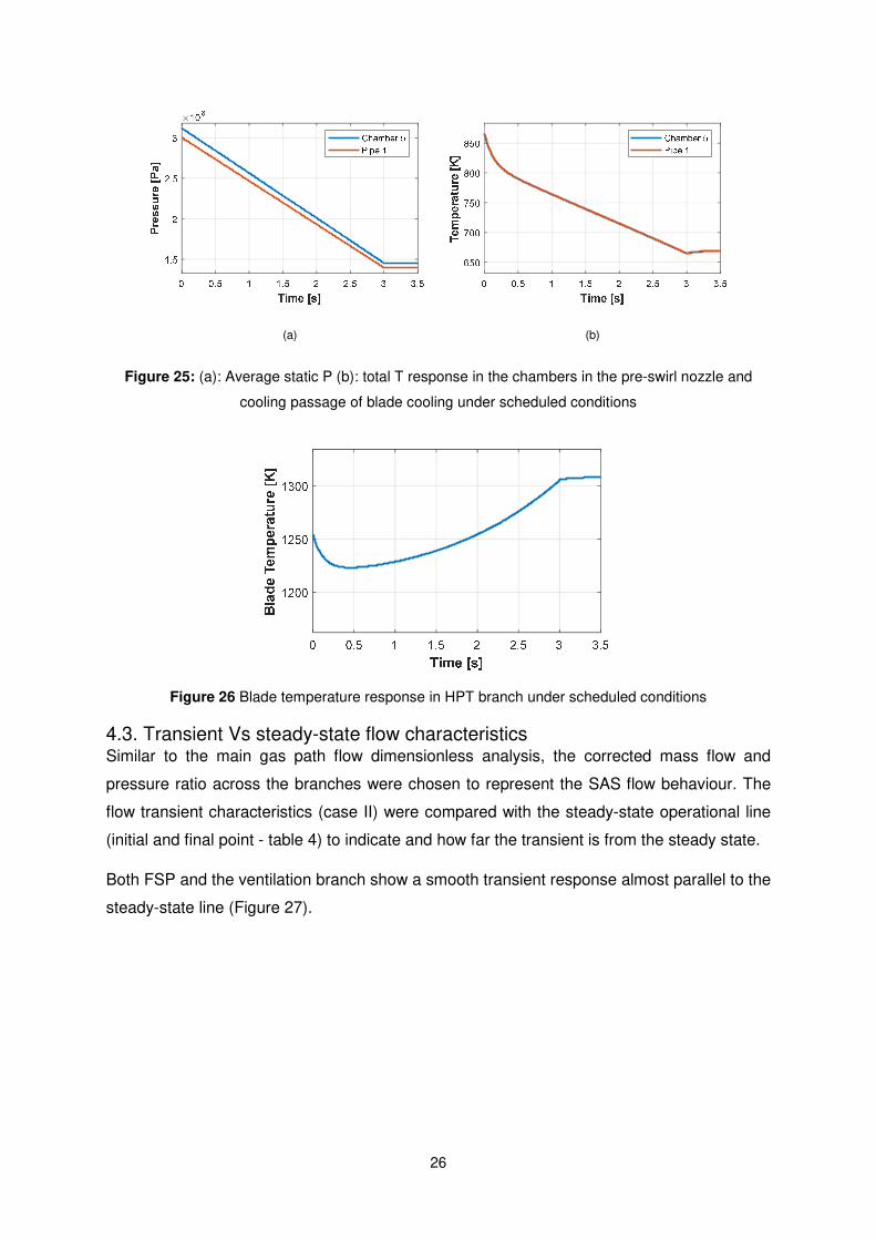
P follow the changes in the boundary conditions for all the branches (Figures 23-25). In this
case, no flow reversal or choking problem was observed. The blade temperature also varies
in a mild way (Figure 26). Therefore, it is sufficient to use steady-state SAS simulate
techniques rather than transient under normal engine operations.
(a) (b)
Figure 23: (a): Average static P (b): total T response in the pipe in FSP branch under scheduled
conditions
(a) (b)
Figure 24: (a): Average static P (b): total T response in the ventilation branch chambers under
scheduled conditions
26
(a) (b)
Figure 25: (a): Average static P (b): total T response in the chambers in the pre-swirl nozzle and
cooling passage of blade cooling under scheduled conditions
Figure 26 Blade temperature response in HPT branch under scheduled conditions
4.3. Transient Vs steady-state flow characteristics Similar to the main gas path flow dimensionless analysis, the corrected mass flow and
pressure ratio across the branches were chosen to represent the SAS flow behaviour. The
flow transient characteristics (case II) were compared with the steady-state operational line
(initial and final point - table 4) to indicate and how far the transient is from the steady state.
Both FSP and the ventilation branch show a smooth transient response almost parallel to the
steady-state line (Figure 27).

27
(a) (b)
Figure 27: Transient performance of (a) FSP & (b) ventilation branch
However, in the HPT rotor cooling branch, a rapid overshooting of mass flow at the starting
point is observed (Figure 28). After the initial period, the transient operating point moves
further away from the steady state operation line. When the boundary conditions are stabilized,
the mass flow converges to the steady-state final value with a small overshooting at the end.
This behaviour is explained by considering the high pressure and temperature at the
boundaries (Figure 25), as well as the non-linear nature of this system.
Figure 28: Transient performance of turbine blade cooling
5. Conclusions An object-oriented SAS simulation platform has been developed by using a modular library for
the different components of the SAS. A flow network simulation has been developed to
replicate the transient behaviour of three main SAS branches in a 2-spool turbofan engine
model under normal and extreme operating conditions. The performance of the critical element
has been validated with public data and reasonable results have been produced using the
platform developed in this paper.
28
It was found that the developed framework is able to predict the behaviour of different
components and branches in the SAS system at different transient operating conditions.
In case of any engine malfunction expressed by an abrupt change in the boundary operating
conditions of the SAS, large flow reversal can take place in the different branches. Additionally,
chocked flow can be observed at the rotor blade cooling branch.
The pressure response is much faster than the temperature. The settling time of pressure is
in the order of 0.001 to 0.01 s, and that of temperature is 0.1 s for the branches tested in this
model. This can vary depending on the complexity of the SAS network (i.e. the number of
branches and individual elements).
The flow performance under scheduled boundary variation (normal operating condition)
transient test is much milder than the abrupt one. Consequently, in the normal operating
condition, a steady-state simulation for the SAS is able to capture the system behaviour very
well. However, the transient simulation would be very helpful in extreme operating conditions
(i.e. shaft fracture, flameout, etc.).

29
Appendix
1. Calculation of �� in equation (6) [14]:
The cumulative moment on the disc can be calculated as: �� = � ��������� dr (A-1)
The derivative of �� over radius r can be obtained as: ����� =5
2���,����ρ��ω����(ω) (A-2)
where ��,���� is the free disc moment coefficient: ��,���� = 0.073����.�(A-3)
and � is the local relative angular velocity between the disc and the air. If the tangential
velocity profile satisfies equation (1), � can be calculated as: ω(�) = ω� − ������(A-4)
where �� is the disc angular velocity. �� is a constant and n is the vortex index, indicating
the vortex behaviour in the chamber [also used in equation (1)]. With this relative velocity being
used, the model developed can be applied to either rotors or stators.
With equation (A-4), the cumulative moment can be obtained:
�� = � 1
2K��,����ρω�(��� − ���) if n = 1
1
2KC�∗ ρω�(��� − ���) if − 1 ≤ n < 1
(A-5)
where � is a constant adjusted to align with the physical system. C�∗ is determined as:
C�∗ = ��,����(a + 1) �ω� − ω�ω� ��∙ ����(ω�)� �ω��� ,
ω���� − ���(ω�)�(ω��� ,
ω���)
(ω� − ω��� )��� � (A-6)
where ω� and ω� are the angular velocity at the inner and outer cavity radius respectively.
Function � and constant � are defined as: �(�, �) = �� ((� − �)��� − ����)� + 1− 2� ((� − �)��� − ����)� + 2
+((� − �)��� − ����)� + 3
(A-7)
� =6 − �� − 1
(A-8)
2. Calculation of �� in equation (6) [14]:
30
�� = ���� 1
2ρω|ω|(2π�����) (A-9)�� = 0.031(2πRe)��/�
(A-10)
where �� is constant adjusted to align with physical conditions. And s� is the length of a
portion of shroud which rotates in �.
3. Calculation of ���� in equation (5) [14]:
Heat input due to disc windage ����,���� is modelled as: ����,disc= �� ∙ Ω� (A-11)
���� due to convection heat transfer is [4]: ����,�� = ℎ�� ∙ �� ⋅ ��� − ����� (A-12)�� is the disc surface area. �� is the area weighted surface temperature and ���� is the
average temperature of the gas. ℎ�� is the surface average heat transfer coefficient and its
determination can be referenced to the appendix in reference [4].
Thus, the total ���� is a sum of the two part in equation (A-11) and (A-12): ���� = ����,���� + ����,�� (A-13)
4. Estimation of carry-over factor � in equation (18) [18][19]:
��� = � 1
1 − �� − 1�� ⋅ �/��/� + 0.02
∙ ���� − 1 (A-14)
where �� represents labyrinth teeth number, c represents teeth clearance and p represents
teeth distance.
5. Calculation of discharge coefficient �� in equation (15) [20]:
The determination of �� is split in several steps. Firstly, a basic value is chosen based on
engineering practice and then it is modified based on Reynolds number (��), corner radius
(��), length (�) and relative tangential velocity (��) effects. The basic value is chosen to be
0.5885.
Firstly, the basic value is modified based on Reynolds number: ��:�� = 0.5885 +372�� (A-15)
Then, it is modified based on corner radius: ��:� = 1 − f ∙ (1 − C�:��) (A-16)
31
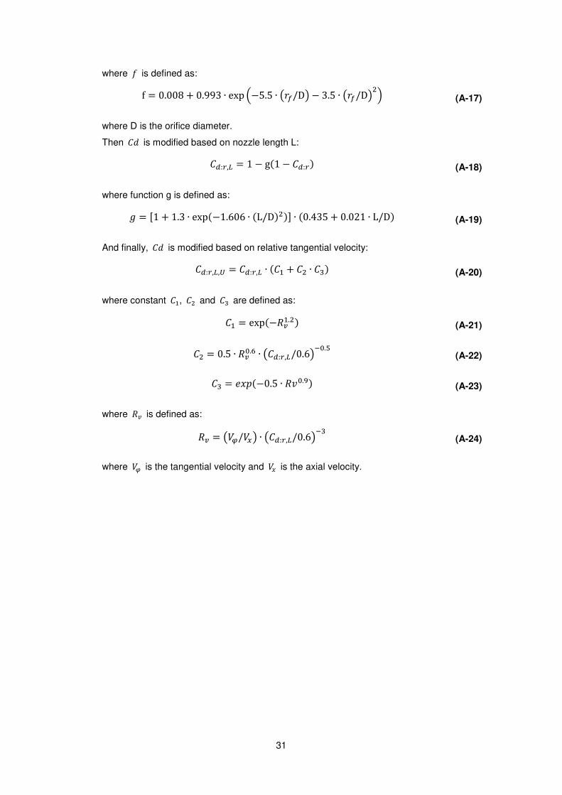
where � is defined as:
f = 0.008 + 0.993 ∙ exp �−5.5 ∙ ���/D� − 3.5 ∙ ���/D��� (A-17)
where D is the orifice diameter.
Then �� is modified based on nozzle length L: ��:�,� = 1 − g(1 − ��:�) (A-18)
where function g is defined as: � = [1 + 1.3 ∙ exp(−1.606 ∙ (L/D)�)] ∙ (0.435 + 0.021 ∙ L/D) (A-19)
And finally, �� is modified based on relative tangential velocity: ��:�,�,� = ��:�,� ∙ (�� + �� ∙ ��) (A-20)
where constant ��, �� and �� are defined as: �� = exp(−���.�) (A-21)�� = 0.5 ∙ ���.� ∙ ���:�,�/0.6���.�(A-22)�� = ���(−0.5 ∙ ���.�) (A-23)
where �� is defined as: �� = ���/��� ∙ ���:�,�/0.6���(A-24)
where �� is the tangential velocity and �� is the axial velocity.

32
References [1] A. Moore, Gas Turbine Engine Internal Air Systems: A Review of the Requirements and
the Problems, ASME 1975 Winter Annu. Meet. GT Pap. (1975) V001T01A001.
doi:10.1115/75-WA/GT-1.
[2] Sultanian, B. (2018), Gas Turbines: Internal Flow Systems Modeling (Cambridge
Aerospace Series), Cambridge: Cambridge University Press,
doi:10.1017/9781316755686
[3] K.J. Kutz, T.M. Speer, Simulation of the Secondary Air System of Aero Engines, J.
Turbomach. 116 (1994) 306. doi:10.1115/1.2928365.
[4] A. Alexiou, K. Mathioudakis, Secondary Air System Component Modeling for Engine
Performance Simulations, J. Eng. Gas Turbines Power. 131 (2009) 031202.
doi:10.1115/1.3030878.
[5] W. Che, S. Ding, C. Liu, A modeling method on aircraft engine based on the Component
Method of secondary air system, Procedia Eng. 80 (2014) 258–271.
doi:10.1016/j.proeng.2014.09.085.
[6] S. Brack, Y. Muller, Probabilistic Analysis of the Secondary Air System of a Low-
Pressure Turbine, J. Eng. Gas Turbines Power. 137 (2014) 022602.
doi:10.1115/1.4028372.
[7] Y. Muller, Secondary Air System Model for Integrated Thermomechanical Analysis of a
Jet Engine, Vol. 4 Heat Transf. Parts A B. (2008) 1359–1374. doi:10.1115/GT2008-
50078.
[8] S. Giuntini, A. Andreini, G. Cappuccini, B. Facchini, Finite element transient modelling
for whole engine-secondary air system thermomechanical analysis, Energy Procedia.
126 (2017) 746–753. doi:10.1016/j.egypro.2017.08.231.
[9] H. Wu, P. Li, Y. Li, Simulation of unsteady state performance of a secondary air system
by the 1D-3D-Structure coupled method, J. Therm. Sci. 25 (2016) 68–77.
doi:10.1007/s11630-016-0835-1.
[10] L. Gallar, Gas Turbine Shaft Over-speed / Failure Performance Modelling, Ph.D thesis,
Cranfield University, 2010. https://dspace.lib.cranfield.ac.uk/handle/1826/8353 .
[11] L. Gallar, C. Calcagni, V. Pachidis, P. Pilidis, Model – Part I : Tool Components Development and Validation, Asme Gt. (2009).
[12] C. Calcagni, L. Gallar, V. Pachidis, Development of a One-Dimensional Dynamic Gas
Turbine Secondary Air System Model—Part II: Assembly and Validation of a Complete
Network, in: 2010: pp. 435–443. doi:10.1115/GT2009-60051.
[13] D. May, J.W. Chew, Response of a Disk Cavity Flow to Gas Turbine Engine Transients,
in: 2010: pp. 1113–1122. doi:10.1115/GT2010-22824.
[14] D. May, J.W. Chew, T.J. Scanlon, Prediction of De-Swirled Radial Inflow in Rotating
Cavities With Hysteresis, in: 2013: pp. 2037–2046. doi:10.1115/GT2012-68647.
[15] M.J. Holland, T.F. Thake, Rotor blade cooling in high pressure turbines, J. Aircr. 17
(1980) 412–418. doi:10.2514/3.44668.
[16] M. Daly, B. Gunston, Jane’s Aero Engines, 2nd ed., IHS Jane’s, 2010.
33
[17] Rolls-Royce, The Jet Engine, 5th ed., Rolls Royce plc, 1996.
[18] B. Hodkinson, Estimation of the Leakage through a Labyrinth Gland, Proc. Inst. Mech.
Eng. 141 (1939) 283–288. doi:10.1243/PIME_PROC_1939_141_037_02.
[19] H. Zimmermann, K.H. Wolff, Air System Correlations: Part 1 — Labyrinth Seals, (1998)
V004T09A048. http://dx.doi.org/10.1115/98-GT-206.
[20] W.F. McGreehan, M.J. Schotsch, Flow Characteristics of Long Orifices With Rotation
and Corner Radiusing, J. Turbomach. 110 (1988) 213. doi:10.1115/1.3262183.
[21] P.R. Farthing, J.W. Chew, J.M. Owen, The Use of Deswirl Nozzles to Reduce the
Pressure Drop in a Rotating Cavity With a Radial Inflow, J. Turbomach. 113 (1991)
106–114. http://dx.doi.org/10.1115/1.2927727.
[22] W. L. Macmillan, Development of a Modular Type Computer Program for the
Calculation of Gas Turbine Off-Design Performance, PhD Thesis, Cranfield Inst. of
Technology, UK, 1974. https://dspace.lib.cranfield.ac.uk/handle/1826/7401.
[23] Th. Nikolaidis, “The TURBOMATCH scheme for Gas Turbine Performance
Calculations,” unpublished software manual, 2017, Cranfield University, UK.
[24] P.R.N. Childs, Mechanical Design, 2nd ed., Elsevier Ltd., 2004.
[25] C. Soria, Gas Turbine Shaft Over-speed / Failure Performance Modelling, Ph.D thesis, Cranfield University, 2014. http://dspace.lib.cranfield.ac.uk/handle/1826/12131.