Transient and Convolution Simulationedadownload.software.keysight.com/eedl/ads/2011/pdf/cktsimtrans.pdf · Transient and Convolution Simulation 1 Advanced Design System 2011 ... HiSIM2

Transient and Convolution Simulation

1

Advanced Design System 2011

September 2011Transient and Convolution Simulation


2

© Agilent Technologies, Inc. 2000-20115301 Stevens Creek Blvd., Santa Clara, CA 95052 USANo part of this documentation may be reproduced in any form or by any means (includingelectronic storage and retrieval or translation into a foreign language) without prioragreement and written consent from Agilent Technologies, Inc. as governed by UnitedStates and international copyright laws.

AcknowledgmentsMentor Graphics is a trademark of Mentor Graphics Corporation in the U.S. and othercountries. Mentor products and processes are registered trademarks of Mentor GraphicsCorporation. * Calibre is a trademark of Mentor Graphics Corporation in the US and othercountries. "Microsoft®, Windows®, MS Windows®, Windows NT®, Windows 2000® andWindows Internet Explorer® are U.S. registered trademarks of Microsoft Corporation.Pentium® is a U.S. registered trademark of Intel Corporation. PostScript® and Acrobat®are trademarks of Adobe Systems Incorporated. UNIX® is a registered trademark of theOpen Group. Oracle and Java and registered trademarks of Oracle and/or its affiliates.Other names may be trademarks of their respective owners. SystemC® is a registeredtrademark of Open SystemC Initiative, Inc. in the United States and other countries and isused with permission. MATLAB® is a U.S. registered trademark of The Math Works, Inc..HiSIM2 source code, and all copyrights, trade secrets or other intellectual property rightsin and to the source code in its entirety, is owned by Hiroshima University and STARC.FLEXlm is a trademark of Globetrotter Software, Incorporated. Layout Boolean Engine byKlaas Holwerda, v1.7 http://www.xs4all.nl/~kholwerd/bool.html . FreeType Project,Copyright (c) 1996-1999 by David Turner, Robert Wilhelm, and Werner Lemberg.QuestAgent search engine (c) 2000-2002, JObjects. Motif is a trademark of the OpenSoftware Foundation. Netscape is a trademark of Netscape Communications Corporation.Netscape Portable Runtime (NSPR), Copyright (c) 1998-2003 The Mozilla Organization. Acopy of the Mozilla Public License is at http://www.mozilla.org/MPL/ . FFTW, The FastestFourier Transform in the West, Copyright (c) 1997-1999 Massachusetts Institute ofTechnology. All rights reserved.

The following third-party libraries are used by the NlogN Momentum solver:

"This program includes Metis 4.0, Copyright © 1998, Regents of the University ofMinnesota", http://www.cs.umn.edu/~metis , METIS was written by George Karypis([email protected]).

Intel@ Math Kernel Library, http://www.intel.com/software/products/mkl

SuperLU_MT version 2.0 - Copyright © 2003, The Regents of the University of California,through Lawrence Berkeley National Laboratory (subject to receipt of any requiredapprovals from U.S. Dept. of Energy). All rights reserved. SuperLU Disclaimer: THISSOFTWARE IS PROVIDED BY THE COPYRIGHT HOLDERS AND CONTRIBUTORS "AS IS"AND ANY EXPRESS OR IMPLIED WARRANTIES, INCLUDING, BUT NOT LIMITED TO, THEIMPLIED WARRANTIES OF MERCHANTABILITY AND FITNESS FOR A PARTICULAR PURPOSEARE DISCLAIMED. IN NO EVENT SHALL THE COPYRIGHT OWNER OR CONTRIBUTORS BELIABLE FOR ANY DIRECT, INDIRECT, INCIDENTAL, SPECIAL, EXEMPLARY, ORCONSEQUENTIAL DAMAGES (INCLUDING, BUT NOT LIMITED TO, PROCUREMENT OF

http://www.xs4all.nl/~kholwerd/bool.html

http://www.xs4all.nl/~kholwerd/bool.html

http://www.mozilla.org/MPL/

http://www.mozilla.org/MPL/

http://www.cs.umn.edu/~metis

http://www.cs.umn.edu/~metis

http://www.intel.com/software/products/mkl

http://www.intel.com/software/products/mkl


3

SUBSTITUTE GOODS OR SERVICES; LOSS OF USE, DATA, OR PROFITS; OR BUSINESSINTERRUPTION) HOWEVER CAUSED AND ON ANY THEORY OF LIABILITY, WHETHER INCONTRACT, STRICT LIABILITY, OR TORT (INCLUDING NEGLIGENCE OR OTHERWISE)ARISING IN ANY WAY OUT OF THE USE OF THIS SOFTWARE, EVEN IF ADVISED OF THEPOSSIBILITY OF SUCH DAMAGE.

7-zip - 7-Zip Copyright: Copyright (C) 1999-2009 Igor Pavlov. Licenses for files are:7z.dll: GNU LGPL + unRAR restriction, All other files: GNU LGPL. 7-zip License: This libraryis free software; you can redistribute it and/or modify it under the terms of the GNULesser General Public License as published by the Free Software Foundation; eitherversion 2.1 of the License, or (at your option) any later version. This library is distributedin the hope that it will be useful,but WITHOUT ANY WARRANTY; without even the impliedwarranty of MERCHANTABILITY or FITNESS FOR A PARTICULAR PURPOSE. See the GNULesser General Public License for more details. You should have received a copy of theGNU Lesser General Public License along with this library; if not, write to the FreeSoftware Foundation, Inc., 59 Temple Place, Suite 330, Boston, MA 02111-1307 USA.unRAR copyright: The decompression engine for RAR archives was developed using sourcecode of unRAR program.All copyrights to original unRAR code are owned by AlexanderRoshal. unRAR License: The unRAR sources cannot be used to re-create the RARcompression algorithm, which is proprietary. Distribution of modified unRAR sources inseparate form or as a part of other software is permitted, provided that it is clearly statedin the documentation and source comments that the code may not be used to develop aRAR (WinRAR) compatible archiver. 7-zip Availability: http://www.7-zip.org/

AMD Version 2.2 - AMD Notice: The AMD code was modified. Used by permission. AMDcopyright: AMD Version 2.2, Copyright © 2007 by Timothy A. Davis, Patrick R. Amestoy,and Iain S. Duff. All Rights Reserved. AMD License: Your use or distribution of AMD or anymodified version of AMD implies that you agree to this License. This library is freesoftware; you can redistribute it and/or modify it under the terms of the GNU LesserGeneral Public License as published by the Free Software Foundation; either version 2.1 ofthe License, or (at your option) any later version. This library is distributed in the hopethat it will be useful, but WITHOUT ANY WARRANTY; without even the implied warranty ofMERCHANTABILITY or FITNESS FOR A PARTICULAR PURPOSE. See the GNU LesserGeneral Public License for more details. You should have received a copy of the GNULesser General Public License along with this library; if not, write to the Free SoftwareFoundation, Inc., 51 Franklin St, Fifth Floor, Boston, MA 02110-1301 USA Permission ishereby granted to use or copy this program under the terms of the GNU LGPL, providedthat the Copyright, this License, and the Availability of the original version is retained onall copies.User documentation of any code that uses this code or any modified version ofthis code must cite the Copyright, this License, the Availability note, and "Used bypermission." Permission to modify the code and to distribute modified code is granted,provided the Copyright, this License, and the Availability note are retained, and a noticethat the code was modified is included. AMD Availability:http://www.cise.ufl.edu/research/sparse/amd

UMFPACK 5.0.2 - UMFPACK Notice: The UMFPACK code was modified. Used by permission.UMFPACK Copyright: UMFPACK Copyright © 1995-2006 by Timothy A. Davis. All RightsReserved. UMFPACK License: Your use or distribution of UMFPACK or any modified versionof UMFPACK implies that you agree to this License. This library is free software; you canredistribute it and/or modify it under the terms of the GNU Lesser General Public License

http://www.7-zip.org/

http://www.7-zip.org/

http://www.cise.ufl.edu/research/sparse/amd

http://www.cise.ufl.edu/research/sparse/amd


4

as published by the Free Software Foundation; either version 2.1 of the License, or (atyour option) any later version. This library is distributed in the hope that it will be useful,but WITHOUT ANY WARRANTY; without even the implied warranty of MERCHANTABILITYor FITNESS FOR A PARTICULAR PURPOSE. See the GNU Lesser General Public License formore details. You should have received a copy of the GNU Lesser General Public Licensealong with this library; if not, write to the Free Software Foundation, Inc., 51 Franklin St,Fifth Floor, Boston, MA 02110-1301 USA Permission is hereby granted to use or copy thisprogram under the terms of the GNU LGPL, provided that the Copyright, this License, andthe Availability of the original version is retained on all copies. User documentation of anycode that uses this code or any modified version of this code must cite the Copyright, thisLicense, the Availability note, and "Used by permission." Permission to modify the codeand to distribute modified code is granted, provided the Copyright, this License, and theAvailability note are retained, and a notice that the code was modified is included.UMFPACK Availability: http://www.cise.ufl.edu/research/sparse/umfpack UMFPACK(including versions 2.2.1 and earlier, in FORTRAN) is available athttp://www.cise.ufl.edu/research/sparse . MA38 is available in the Harwell SubroutineLibrary. This version of UMFPACK includes a modified form of COLAMD Version 2.0,originally released on Jan. 31, 2000, also available athttp://www.cise.ufl.edu/research/sparse . COLAMD V2.0 is also incorporated as a built-infunction in MATLAB version 6.1, by The MathWorks, Inc. http://www.mathworks.com .COLAMD V1.0 appears as a column-preordering in SuperLU (SuperLU is available athttp://www.netlib.org ). UMFPACK v4.0 is a built-in routine in MATLAB 6.5. UMFPACK v4.3is a built-in routine in MATLAB 7.1.

Qt Version 4.6.3 - Qt Notice: The Qt code was modified. Used by permission. Qt copyright:Qt Version 4.6.3, Copyright (c) 2010 by Nokia Corporation. All Rights Reserved. QtLicense: Your use or distribution of Qt or any modified version of Qt implies that you agreeto this License. This library is free software; you can redistribute it and/or modify it undertheterms of the GNU Lesser General Public License as published by the Free SoftwareFoundation; either version 2.1 of the License, or (at your option) any later version. Thislibrary is distributed in the hope that it will be useful,but WITHOUT ANY WARRANTY; without even the implied warranty of MERCHANTABILITYor FITNESS FOR A PARTICULAR PURPOSE. See the GNU Lesser General Public License formore details. You should have received a copy of the GNU Lesser General Public Licensealong with this library; if not, write to the Free Software Foundation, Inc., 51 Franklin St,Fifth Floor, Boston, MA 02110-1301 USA Permission is hereby granted to use or copy thisprogram under the terms of the GNU LGPL, provided that the Copyright, this License, andthe Availability of the original version is retained on all copies.Userdocumentation of any code that uses this code or any modified version of this code mustcite the Copyright, this License, the Availability note, and "Used by permission."Permission to modify the code and to distribute modified code is granted, provided theCopyright, this License, and the Availability note are retained, and a notice that the codewas modified is included. Qt Availability: http://www.qtsoftware.com/downloads PatchesApplied to Qt can be found in the installation at:$HPEESOF_DIR/prod/licenses/thirdparty/qt/patches. You may also contact BrianBuchanan at Agilent Inc. at [email protected] for more information.

The HiSIM_HV source code, and all copyrights, trade secrets or other intellectual propertyrights in and to the source code, is owned by Hiroshima University and/or STARC.

http://www.cise.ufl.edu/research/sparse/umfpack

http://www.cise.ufl.edu/research/sparse/umfpack

http://www.cise.ufl.edu/research/sparse




http://www.mathworks.com

http://www.mathworks.com

http://www.netlib.org

http://www.netlib.org

http://www.qtsoftware.com/downloads

http://www.qtsoftware.com/downloads


5

Errata The ADS product may contain references to "HP" or "HPEESOF" such as in filenames and directory names. The business entity formerly known as "HP EEsof" is now partof Agilent Technologies and is known as "Agilent EEsof". To avoid broken functionality andto maintain backward compatibility for our customers, we did not change all the namesand labels that contain "HP" or "HPEESOF" references.

Warranty The material contained in this document is provided "as is", and is subject tobeing changed, without notice, in future editions. Further, to the maximum extentpermitted by applicable law, Agilent disclaims all warranties, either express or implied,with regard to this documentation and any information contained herein, including but notlimited to the implied warranties of merchantability and fitness for a particular purpose.Agilent shall not be liable for errors or for incidental or consequential damages inconnection with the furnishing, use, or performance of this document or of anyinformation contained herein. Should Agilent and the user have a separate writtenagreement with warranty terms covering the material in this document that conflict withthese terms, the warranty terms in the separate agreement shall control.

Technology Licenses The hardware and/or software described in this document arefurnished under a license and may be used or copied only in accordance with the terms ofsuch license. Portions of this product include the SystemC software licensed under OpenSource terms, which are available for download at http://systemc.org/ . This software isredistributed by Agilent. The Contributors of the SystemC software provide this software"as is" and offer no warranty of any kind, express or implied, including without limitationwarranties or conditions or title and non-infringement, and implied warranties orconditions merchantability and fitness for a particular purpose. Contributors shall not beliable for any damages of any kind including without limitation direct, indirect, special,incidental and consequential damages, such as lost profits. Any provisions that differ fromthis disclaimer are offered by Agilent only.

Restricted Rights Legend U.S. Government Restricted Rights. Software and technicaldata rights granted to the federal government include only those rights customarilyprovided to end user customers. Agilent provides this customary commercial license inSoftware and technical data pursuant to FAR 12.211 (Technical Data) and 12.212(Computer Software) and, for the Department of Defense, DFARS 252.227-7015(Technical Data - Commercial Items) and DFARS 227.7202-3 (Rights in CommercialComputer Software or Computer Software Documentation).

http://systemc.org/

http://systemc.org/


6

About Transient and Convolution Simulation . . . . . . . . . . . . . . . . . . . . . . . . . . . . . . . . . . . . . 7 Performing a Transient or Convolution Simulation . . . . . . . . . . . . . . . . . . . . . . . . . . . . . . . . . 8 Examples of Transient and Convolution Simulation . . . . . . . . . . . . . . . . . . . . . . . . . . . . . . . . . 9 Transient and Convolution Simulation Description . . . . . . . . . . . . . . . . . . . . . . . . . . . . . . . . . 13 Monte-Carlo Noise in the Time Domain . . . . . . . . . . . . . . . . . . . . . . . . . . . . . . . . . . . . . . . . . 18 Transient Simulation Parameters . . . . . . . . . . . . . . . . . . . . . . . . . . . . . . . . . . . . . . . . . . . . . 19 Troubleshooting a Transient-Convolution Simulation . . . . . . . . . . . . . . . . . . . . . . . . . . . . . . . . 29


7

About Transient and ConvolutionSimulation Transient Convolution Simulator solves a set of integro-differential equations that expressthe time dependence of the currents and voltages of the circuit. The result of such ananalysis is nonlinear with respect to time and, possibly, a swept variable. In ADS, thiscontroller is available in the Simulation-Transient palette.

Transient Convolution Simulator enables you to:

Perform a SPICE-type transient time-domain analysis on a circuit.Perform nonlinear transient analysis on circuits that include the frequency-dependentloss and dispersion effects of linear models such as S-parameter models. Suchanalyses are known as convolution analyses.

Refer to these topics:

Performing a Transient or Convolution Simulation (cktsimtrans) has the minimumsetup requirements for a transient simulation.Examples of Transient and Convolution Simulation (cktsimtrans) has a detailed setupfor performing a transient simulation, using a Gilbert cell mixer as the example.Transient and Convolution Simulation Description (cktsimtrans) is a brief explanationof transient and convolution simulations.Transient Simulation Parameters (cktsimtrans) provides details about the parametersavailable in the Transient simulation controller in ADS.Troubleshooting a Transient-Convolution Simulation (cktsimtrans) offers suggestionson how to improve a simulation.

NoteYou must have licenses for either the W2302 Transient Convolution Simulator Element or both E8884High Frequency SPICE (transient simulator) and the E8885 Convolution Simulator or a bundle containingthese to run these types of simulations. You may build the examples without the appropriate license, butcannot run the simulations.


8

Performing a Transient or ConvolutionSimulation Start by creating your design, then add current probes and identify the nodes from whichyou want to collect data.

For a successful analysis:

When selecting sources, you can use either frequency-domain or time-domainsources. Transient sources are under the Sources-Time Domain palette. They areidentified by the small t in their names (for example, VtStep:Voltage Source: Step).Add the Trans component to the schematic. Double-click to edit it. Fill in the fieldsunder the Time Setup tab:

Enter the start and stop times.Enter the Max time step. This is the largest time step that will be used in thesimulation. It should be small enough to adequately sample the highestfrequency expected in the circuit.

To achieve the most accurate model, select the Convolution tab and set the MaxFrequency and max impulse sample points. The other parameters here are related togenerating impulse responses for convolution analysis, but in general accept thedefaults. For more information, refer to the sections Convolution Analysis(cktsimtrans) and Setting Max Frequency and Other Convolution Parameters(cktsimtrans).If frequency is not defined by a frequency source, select the Freq tab and set thefundamentals and order.The parameters under the Integration tab set truncation, integration techniques, andcharge accuracy. For information on integration techniques, see Integration MethodsUsed in Transient-Convolution Simulation (cktsimtrans).The parameters under the Convergence tab are used to improve convergence. Formore information, see Solving Convergence Problems (cktsimtrans).You can use the steady state detector to find out the steady state conditions of acircuit. See Using the Steady State Detector and Transient Assisted HarmonicBalance (cktsimtrans).It is recommended that parameters not specifically mentioned here be left at thedefault values. For more information about each parameter, click Help in the Transdialog box.


9

Examples of Transient and ConvolutionSimulation This section provides an example using a Gilbert cell mixer, and lists other examplesshipped with ADS that demonstrate transient simulations with other types of circuits.

The following figure illustrates the setup for a basic transient/convolution simulation.

NoteThis design, TRAN1, is in the Examples directory under Tutorial/SimModels_wrk. The results are inTRAN1.dds.

Setup for Transient/Convolution simulation

To perform a basic transient/convolution simulation:

From the Component Palette, choose Sources-Time Domain or Sources-Freq1.Domain and select appropriate sources. Place the source at the input of thecomponent or circuit under test, then define input power and edit other parametersas required. In a circuit employing a mixer, provide a source for the local oscillator(LO).

NoteTransient sources, available in the Time Domain Sources palette, are available for these simulations,and are identified by the small "t" in their names (for example, VtStep:Voltage Source: Step).However, standard frequency sources (in the Freq Domain Source palette) can also be used.

Ensure that the inputs and outputs of nodes at which you want data to be reported2.are appropriately labeled.


10

If they are needed, select from among various transient measurement equations in3.the Transient Simulation palette, place these on the schematic, and edit them asrequired. (See Troubleshooting a Transient-Convolution Simulation (cktsimtrans).)Their results can be plotted later in a Data Display window.From the Component Palette, choose Simulation-Transient. Select and place the4.Tran simulation component on the schematic. You can run a basic simulation byediting the parameters StopTime and MaxTimeStep on the schematic.

NoteThe Max time step value should be small enough to adequately sample the highest frequencyexpected in the circuit. The simulator may use a smaller timestep if needed but will never use alarger value.

To edit the frequency of the fundamental and any other frequencies to be considered,5.select the Freq tab. This frequency information is required only if the frequency is notset explicitly in the frequency domain sources.The parameters that make it possible to obtain the most accurate model are Max6.Frequency and Max impulse sample points, under the Convolution tab of thesimulation component. It is recommended that you leave the other parameters underthis tab at their default settings and edit them only in special cases.For details regarding all Transient parameters, double-click the simulation component7.to edit it, select the tab of interest, and click the Help button. Many parameters inthis simulator apply only to special cases.Launch the simulation. The data resulting from this simulation will be identified by8.TRAN1. The large trace is a plot of Vif versus time, the output of the filter showing allharmonic components. The small sinusoid is a plot of Vload following the filter. Thefilter output has been given enough time to approach a steady-state amplitude.

A plot of fs(Vif,,,,,,,4ns,16ns) shows a time-to-frequency transform from 4 to 16 ns9.for the mixer output before filtering. (The seven commas represent fs parameters notused here.) Run the simulation longer to observe the noise floor drop.

Finally, an fs plot of the filter output (Vload) between 24 and 32 ns shows the10.


11

response after steady-state amplitude has been approximated. Essentially only thebandpass frequency remains.

Additional ADS Examples

For a list of additional examples demonstrating transient simulation, see the followingtable. The table gives you the locations of their descriptions in the Examplesdocumentation, and the location of the example workspaces available in the$HPEESOF_DIR/examples directory.


12

Example DocumentationLocation

Example Workspace Location

Cosimulation ofBaseband Sine Waveand Amplifier Circuit

Examples >Communication Systems> Baseband Sine Waveand AmplifierCosimulation

/examples/Com_Sys/Co_Sim_wrk/Co_sim_1

Frequency and TimeDomain Simulation ofMulti-CoupledMicrostrip Lines

Examples > RF Board >Multi-Coupled MicrostripLines

/examples/RF_Board/MultilayerMeas_wrk/

Basic PLL Simulationusing Circuit Envelope

Examples > RF Board >PLL Examples > PLLSimulations using CircuitEnvelope

/examples/RF_Board/PLL_Examples/PLL_VideoExamples_wrk

TDR and S-parameterSimulations ofMicrostrip StepDiscontinuities

Examples > RF Board >Microstrip StepDiscontinuities

/examples/RF_Board/TDRmeas_vs_model_wrk

Various Simulationsof A Power Amplifier

Examples > RFIC >Power Amplifier

/examples/RFIC/amplifier_wrk

RFIC OscillatorSimulations

Examples > RFIC >RFIC Oscillator

/examples/RFIC/RFICoscillator_wrk

Oscillator Simulationsusing Transient,Harmonic Balanceand EnvelopeSimulators

Examples > Tutorial >Oscillator Simulations

/examples/Tutorial/Osc_Tran_HB_Env_wrk


13

Transient and Convolution SimulationDescriptionThe transient and convolution simulators are SPICE-like in their operation. They solve aset of integro-differential equations that express the time dependence of the currents andvoltages of the circuit under analysis. The result is a nonlinear analysis with respect totime and, possibly, a swept variable.

The main difference between the transient and convolution options lies in how eachanalysis characterizes the distributed and frequency-dependent elements of a circuit, asdiscussed below.

Transient Analysis

A transient analysis is performed entirely in the time-domain, and so is unable to accountfor the frequency-dependent behavior of distributed elements such as microstripelements, S-parameter elements, and so on. Therefore, in a transient analysis, suchelements must be represented by simplified, frequency-independent models such aslumped equivalents, transmission lines with constant loss and no dispersion, short circuits,open circuits, and the like. These assumptions and simplifications are usually veryreasonable at low frequencies.

Convolution Analysis

A convolution analysis represents all the distributed elements in the frequency domain andhence accounts for their frequency-dependent behavior. The characterization of many RFand microwave distributed elements is best accomplished in the frequency domain,because the exact time-domain equivalents for these elements cannot always be obtained.

Convolution converts the frequency-domain information from all the distributed elementsto the time domain, effectively resulting in the impulse response of those elements. Thetime-domain input signals at an element's terminals are convolved with the impulse-response of the element to yield the output signals. Elements that have exact lumpedequivalent models-including nonlinear elements-are characterized entirely in the timedomain without using impulse responses.

NoteIn a convolution analysis, all elements are characterized by means of the full frequency-domain model,through the use of either an exact time-domain model or convolution. However, there may be minordifferences between the results of a convolution simulation and the results of a transient simulation of thesame circuit.

A convolution analysis requires both a convolution license and a transient license, and isperformed whenever a convolution license is available. If the simplified approximate


14

models are preferred, in this situation (for speed), set the Use Approximate Models WhenAvailable option to yes.

Transient/Convolution Simulation Process

The following steps describe how both the transient and convolution simulators operate:

The user specifies a time-sweep range, tolerances, and iteration limits.1.A DC analysis is conducted to determine the system solution at zero time.2.Inside the simulator, a breakpoint table is constructed to deal with frequency-3.domain-devices and data. Independent source waveforms frequently have sharptransitions that may not normally coincide with the time step calculated by theprogram. Such is the case with the piecewise linear sources. The breakpoint tablecontains a sorted list of all the transition points of the independent sources. Duringthe simulation, whenever the next time point is sufficiently close to one of thebreakpoints, the time step is adjusted to land exactly on the breakpoint. Thisprevents unnecessary time-step reductions in the vicinity of the transitions.An internal control variable updates the current time, and the values of the4.independent sources are calculated at that time.An attempt is made to solve the system of equations through numerical integration5.and a finite number of Newton-Raphson iterations. If the number of iterationsexceeds Max iterations per time point, then the time step is reduced by a factor ofIntegration coefficient mu divided by 8. If this new time step is acceptable, theanalysis is repeated from step 4. If Integration coefficient mu = 0, backward-Eulernumerical integration is used. Otherwise, trapezoidal numerical integration is used.Following convergence, the local truncation error is calculated. The default6.Trapezoidal integration method is used to estimate the error, unless Gear's method isselected.The time step interval is calculated. By default, the time step is computed for7.transient analysis by means of the truncation error estimate method.The error tolerance is compared with the value in the Local truncation error over-est8.factor field (under the Integration tab). If the error is within acceptable limits, theresults are stored and analysis continues at the next time point. Otherwise, theanalysis is repeated at a smaller time step.Steps 3 through 9 are repeated until the user-specified time-sweep range has been9.analyzed.

Time Step Control Characteristics

These are the specific characteristics for time step control.Local Truncation Error:

Estimates the LTE made on every capacitor and inductor.Determines the time step size to ensure the largest LTE remains within the acceptedtolerance.The estimated LTE is inversely proportional to TruncTol.


15

The accepted tolerance is proportional to I_RelTol x TruncTol and V_RelTol xTruncTol.

Iteration-Count:

Determines the time step size based on the number of Newton iterations required forprevious time point.No direct relationship between iterations and LTE.Effectively controlled by Max time step (for linear circuits).

Fixed:

The time step is fixed and equal to Max time step.

Break Points:

Generated by built-in independent sources whenever an abrupt change in slopeoccurs.Ensure that corners in waveforms are not missed.ADS always places time points on a break point (except fixed time step).Backward Euler is used on time points that are the first time step after break points.The step size is reduced when time point is close to a break point.

Integration Methods Used in Transient-Convolution Simulation

Like SPICE, this simulator uses the trapezoidal integration method described by thefollowing equation as the default method for calculating derivatives at each time step t inthe simulation.

For most circuits, this method will succeed. For those that do not, the simulator alsosupports Gear's backward difference method:

In this equation, the index k is called the order of the integration.

For most circuits, Gear's method is no more accurate than the default trapezoidalintegration technique. However, if a circuit analysis fails to converge, Gear's method maysucceed where trapezoidal integration fails. In particular, oscillator circuits and any circuitthat is characterized by stiff state equations may benefit from Gear's method.


16

NoteFor a discussion of Gear's method and stiff state equations, refer to Chua and Lin, Computer-AidedAnalysis of Electronic Circuits: Algorithms and Computation Techniques, Prentice-Hall, 1975.

If Time Step Control is set to TruncError and Max Gear order (under the Integration tab) isset to a number between two and six, the simulator will use Gear's method along with anadaptive stepsize algorithm that picks the largest possible step size at each point in thesimulation. For each time step, the order of Gear's method will be chosen (up to the valueof Max Gear order ) to maintain accuracy with the largest possible time step. Thispotentially speeds up simulations with no loss in accuracy. If Gear Integration is selectedwith fixed timestep, then the integration will always be done at the fixed order given byMax Gear order.

The integration order at each time step is output to the dataset as the variable tranorder.This data is used by the fs() function, in data display, to do accurate interpolation of thedata when an FFT is required. For the default trapezoidal integration, this will normallyhave a value of two, except at source-induced breakpoints where it will be one.

Using the Steady State Detector and Transient Assisted Harmonic Balance

You can perform a transient simulation with the steady state detector to find out thesteady state conditions of a circuit. This includes whether or not steady state was reached,the time at which steady state was reached, and the frequency of oscillation in the eventof having an oscillator circuit. To get this information, enable the Detect Steady Stateparameter and enter the frequency of the source that is driving the circuit for Freq[1] (orthe potential oscillation frequency for an autonomous circuit). The resulting steady statevalues will appear in the ADS status window.

The Transient simulator may also be used to generate an initial guess for a harmonicbalance simulation. For circuits that are highly nonlinear and contain sharp-edgedwaveforms (such as dividers), a transient simulation often provides a good initial guess forthe starting point of harmonic balance.

Transient assisted harmonic balance is automated and can be set to Auto, On, or Offmode from the TAHB tab on the Harmonic Balance simulation controller. However, if youprefer to perform a manual TAHB simulation, there are two ways to do it.

On the Freq tab, fill in the frequency fields as you would for a harmonic balancesimulation. The Frequency values can still be used, independent of this solution mode, todefine the fundamental frequencies and _freqN variables used in sources. The Order andMaximum order information is used to determine the number of frequencies for which tocompute a harmonic balance solution.

The first way is to enable the steady state detector and allow the transient simulator tocapture the steady state portion of the solution waveforms. When taking this approach, besure to give at least one the frequency and order parameter (Freq[1], Order[1]), andselect the box labeled Write initial guess for HB. The transient simulator will reportwhether or not steady state was reached, and if so, the time at which it was reached and


17

frequency of oscillation (when simulating an oscillator). The simulator will stop oncesteady state has been reached and transform just the last period of the solution.

The second way is to manually adjust the StartTime and StopTime to capture the steadystate portion of the solution. As with the first method, at least one frequency and orderparameter (Freq[1], Order[1]) must be given and Write initial guess for HB should beselected. The time to frequency domain transform does not start until after StartTime hasbeen reached, so set StartTime appropriately so that the non-steady state portion is nottransformed. StopTime should be set so at least one full period of the steady statesolution occurs after StartTime. Set MaxTimeStep small enough to accommodate thelargest signal frequency. With this approach, it is recommended to plot the transientresults in the data display and verify that the waveforms are very near steady state. Forbest results, especially in multi-tone applications, enable Apply Window. This applies awindow to the time domain data. This window helps to minimize the spectral leakagewhen multiple frequency tones are present.

In both cases, the name for the initial guess file should also be entered for the Fileparameter.

For circuits with multiple sources, it is strongly recommended to do a single tone transientsimulation when generating the initial guess for harmonic balance. In other words, useonly Freq[1] and Order[1] when setting up the fundamental frequency for a Transientsimulation. This should be the most nonlinear tone. This is typically the tone with thelargest power that would drive the circuit into compression.


18

Monte-Carlo Noise in the Time DomainNoise in transient simulations can be added as pseudo-random voltages and currents ateach timepoint. The noise has a Gaussian amplitude distribution. The noise can befrequency- or bias-dependent, as appropriate for each component. All components thatgenerate noise in a linear or harmonic balance simulation generate the appropriate noise,with the following exceptions:

S-parameter data from files that include a noise parameter block with NFmin, Rn andSoptBehavioral components for amplifiers and mixersNoisy2Port componentNoiseCorr noise correlation componentSDDMextram504 and Hicum transistor models

The noise is added to the signal, so there is no easy way to separate the signal from thenoise. The full, nonlinear circuit equations are applied to this composite signal of randomvoltages and currents, so no small-signal assumptions about the relative size of the noiseare required.

The Noise bandwidth parameter (under the Transient Noise tab) enables the generation ofnoise in transient analysis. Because transient analysis uses a variable timestep method,the noise must be limited to a bandwidth of less than 1/(2*MaxTimeStep). If thisparameter is left blank or specified as zero, no noise is generated.

The Noise scale parameter is used to multiplicatively scale all of the noise sources in thecircuit. This can be useful when the noise levels are very low, as this allows them to beincreased so they are visible above the numerical noise in the simulation. However, if thenoise is increased too much, it can change the nonlinear operation of the circuit.

The noise is generated by a random number generator. It will produce a differentsequence of random numbers each time the simulation is run. If a repeatable sequence isrequired, it can be obtained by setting the simulator variable __randseed to an integervalue with a schematic equation. For example,

__randseed=12345 (two underscores precede randseed)


19

Transient Simulation Parameters ADS provides access to Transient simulation parameters enabling you to define aspects ofthe simulation listed in the following table:

Tab Name Description For details, see...

Time Setup Sets parameters related to time and frequency. Defining the Time Setup

Integration Selects an integration mode and sweep offset, turns on sourceand resistor noise, and sets device-fitting parameters. Optionsfor oscillator analysis are also available.

Setting the IntegrationMethod

Convolution Sets parameters related to convolution analysis setup.Includes access to advanced convolution options.

Setting Up ConvolutionAnalysis

Convergence Sets parameters related to achieving convergence. Setting Up the Convergence

Options Sets parameters related to simulation reporting levels andsaving operating point level data.

Setting Up OptionalParameters

Noise Sets noise bandwidth and scale. Defining the Noise Parameters

Freq Sets parameters for the fundamental frequencies which are usedfor computing an initial guess for a harmonic balance simulation.This approach is called Transient-Assisted Harmonic Balance(TAHB).

Setting the FundamentalFrequencies

Output Selectively save simulation data to a dataset. For details, see SelectivelySaving and ControllingSimulation Data (cktsim).

Display Control the visibility of simulation parameters on the schematic. For details, see DisplayingSimulation Parameters on theSchematic (cktsim).

Using Transient Parameters in ADS

When using this controller, here are tips about preparing your design for simulation:

While ten Transient parameters affect convolution, some components allow eight ofthese parameters to be set individually for the component.Component values override those on the controller.Whenever possible, set values on the component.Don't restrict adaptive impulse calculation except where needed.Don't limit Max Frequency (ImpMaxFreq) for all components if only one componentrequires a limit.

Setting Initial Conditions with InitCond Components

There are two elements for setting initial conditions in a transient simulation InitCond andInitCondbyName. InitCond and InitCondByName are used to provide an initial DC value fortransient analysis only. These elements attach the specified voltage source with a series


20

resistor to the specified node(s) to force a value. The DC solution for the entire circuit isthen calculated. This DC solution is then used as the starting state for the transientanalysis.

Defining the Time Setup

Following is information on the parameters related to time and frequency. The followingtable describes the parameter details. Names listed in the Parameter Name column areused in netlists and on schematics.

Transient Simulation Time Setup Parameters

Setup Dialog Name ParameterName

Description

Output Times

Start time StartTime The time at which the simulator begins outputting time-pointresults. This enables control over large amounts of output data.

Stop time StopTime The time at which the simulator stops outputting time-point results.Must be long enough if steady state is needed. You must specify thisparameter.

Max time step MaxTimeStep The largest time step to be taken in the simulation. You must specifythis parameter.

Min time step MinTimeStep The smallest time step to be taken in the simulation. Generally thedefault value is satisfactory.

Limit timestep forTransmission Line

LimitStepForTL Where transmission lines are involved, setting this option furtherlimits the time step to half of the shortest transmission line's delaytime.

Setting the Integration Method

Following is information on setting up the Integration portion of the simulation. Thefollowing table describes the parameter details. Names listed in the Parameter Namecolumn are used in netlists and on schematics.

Transient Simulation Integration Parameters


21

Setup DialogName

ParameterName

Description

Time stepcontrolmethod

TimeStepControl

Fixed Fixed Selects a fixed time-step method. The simulation is performed with auniform, constant time step that is specified by Max time step (under theTime Setup tab). It is quicker than the other methods. However, it is not asrobust, because it cannot select a smaller time step when convergenceproblems are encountered.

IterationCount

Iteration Count Uses the number of Newton-Raphson iterations that were needed toconverge at a time point as a measure of the rate of change of the circuit.If the number of iterations is less than an internal threshold, the time stepis doubled; if the number is greater than Max iterations per time step, thetime step is scaled by a factor of Integration coefficient mu divided by 8(see below). This method has a minimal computational overhead, but doesnot take into account the true rate of change of circuit variables. Use this ifno energy storage component is present and the Local truncation error isnot checked.

Trunc Error Trunc Error Default. Uses the current estimate of local truncation error to determine anappropriate time step. Although it takes longer than Iteration count, it setsa meaningful error bound on computed output values.

Localtruncationerror over-estfactor

TruncTol A value against which the simulation's error tolerance is compared. Intransient analysis each time step is computed by means of the truncation-error estimate method. If the error is within acceptable limits, the resultsare stored and analysis continues at the next time point. Otherwise, theanalysis is repeated at a smaller time step. Increase this value to relax localtruncation error convergence tolerance without relaxing the Newtoniteration convergence tolerance.

Chargeaccuracy

ChargeTol The minimum charge value used to determine the charge tolerance whencomputing the local truncation error. Default = 1e-14.

Integration IntegMethod

Trapezoidal Trapezoidal Default. Integrates between time points by assuming they are connected byline segments. The local truncation error is then related to the differencebetween the areas determined by the present and previous time points.

Gear's Gear's Integrates by assuming that the time points are connected by a polynomialcurve. The order of the polynomial is controlled by the Max Gear orderparameter. Lower-order polynomials tend to create greater truncationerror, while higher-order polynomials can become unstable.

Max Gearorder

MaxGearOrder Determines the maximum order of the polynomial when Gear's method isused. The default is 2. This is available only when Gear's is selected.

Integrationcoefficientmu

Mu A coefficient that determines the degree of mixing of the trapezoidal (mu =0.5) and backward-Euler (mu = 0.0) methods when the trapezoidal methodis used. This is available only when Trapezoidal is selected. The valid rangefor mu is: 0.0 <= mu <= 0.5.Caution: Do not set mu to 1.0; this results in a divide-by-zero condition.The integration order at each timestep is output to the dataset as thevariable tranorder. This data is used by the fs() function in the data displayserver to do accurate interpolation of the data when an FFT is required. Forthe default trapezoidal integration, this will normally have a value of 2,except at source-induced breakpoints where it will be 1.


22

Setting Up Convolution Analysis

Following is information on setting up the Convolution portion of the simulation. Thefollowing table describes the parameter details. Names listed in the Parameter Namecolumn are used in netlists and on schematics.

Notes

It is recommended that the Convolution parameters are left at their default settings.1.Convolution in Transient controller can be set to behave the same as in Channel Simulation by2.setting the same value for overlapping parameters and default values for non-overlappingparameters.

Transient Simulation Convolution Parameters

SetupDialogName

Parameter Name Description

Tolerance - Sets the tolerance for relative and absolute truncation factors for the impulse response:ImpRelTrunc and ImpAbsTrunc. Values are set depending on the option selected for Tolerance. Auto is thedefault. ImpRelTrunc default value is 1e-4. ImpAbsTrunc default value is 1e-7, and it controls how small theimpulse must be before it is considered zero.

Relax When selected, impulse response truncation factors are set to the following:ImpRelTrunc = 1e-2ImpAbsTrunc = 1e-5

Auto Default setting. Default values are used for ImpRelTrunc=1e-4, andImpAbsTrunc=1e-7.

Strict When selected, impulse response truncation factors are set to the following:ImpRelTrunc = 1e-6ImpAbsTrunc = 1e-8

EnforcePassivity

ImpEnforcePassivity Default setting is on (selected). When selected, this option enforces passivityfor linear frequency domain components which are simulated using discretemode convolution. Similarly, if EnforcePassivity=yes in a SnP component,passivity will be enforced in that particular device. The EnforcePassivitysetting of SnP component overwrites the ImpEnforcePassivity setting of thetransient controller in an individual device. Therefore, if a SnP component isactive by design, EnforcePassivity should be disabled by settingEnforcePassivity=No in that paticular SnP component.

Advanced Click Advanced on the Convolution tab to set these parameters. Forparameter descriptions, see Defining Advanced Convolution Parameters</ahref>.

Defining Advanced Convolution Parameters

Use the following parameters for additional control of convolution simulations.

Advanced Convolution Options


23

Setup DialogName

Parameter Name Description

Useapproximatemodels whenavailable

ImpApprox Causes the simulator to bypass impulse-based convolution (whenthat option is available to you). Instead, it uses models that,although somewhat less accurate, can provide faster simulations.These approximations neglect effects such as frequency-dependentloss and dispersion, but include the basic delay and impedance.These models are the default, if no convolution license is available.Default setting is unselected.

Approximateshorttransmissionlines

ShortTL_Delay Specifies a limit on the time delay below which transmission lineswill be approximated instead of modeled as a delay line. Thisenables you to analyze very short transmission lines with a Laplacetransform approximation. Also, it does not require the simulator totake the very small time steps normally associated with shorttransmission lines. Only single, two terminal, transmission lines(like MLIN and TLIN, but not MCLIN and TLIN4) can beapproximated this way.

Max Frequency ImpMaxFreq The maximum frequency to which a frequency-domain device isevaluated to obtain its impulse response. By default, the programchooses this value according to signal source bandwidth. You donot normally need to set this, unless it is necessary to increase it tomodel the high frequency components due to circuit nonlinearity.

DeltaFrequency

ImpDeltaFreq The frequency interval between samples in the evaluation offrequency-domain-defined devices.

Save ImpulseSpectrum

ImpSaveSpectrum Saves the impulse response, its FFT, and the original spectrum to adataset when discrete mode convolution is used in transientanalysis. The default value is no (unselected). The informationadded to the dataset uses names similar to those shown herewhere CMP1 is the component name:CMP1_FFT_IMP: FFT of final impulse response used in convolution.CMP1_IMP: Final impulse response used in convolution.CMP1_OR: Original spectrum.CMP1_S0: Exists only if passivity is enforced. Spectrum aftercausality but before passivity correction.

Enforce StrictPassivity

ImpEnforceStrictPassivity Default is off (unselected). This option takes effect only whenregular "Enforce Passivity" is selected and the Enforce StrictPassivity check box is selected. This option is recommended ifconvolution fails to converge when the regular (non-strict) EnforcePassivity option is used. Although such failure is rare, it can happenparticularly if a linear frequency domain component has a largenumber of ports. When "Strict" is selected, passivity is alsoenforced in the high frequency extrapolation region. Therefore,impulse response calculation is slower but convergence is morereliable.

Backward Compatibility for Convolution

Due to the improved convolution simulation algorithm in ADS 2008 the parameters listedin the following table that were available in previous releases are obsolete. Parameters forConvolution Mode and Tolerance will be handled in ADS 2008 as described here:

ADS 2008 always uses Discrete mode for Convolution Mode (ImpMode) and the PWLContinuous mode is disabled. If a design from a previous release uses PWLContinuous mode, ADS 2008 automatically sets the parameter to Discrete mode.In designs created in a previous release, the values of parameters supported by ADS


24

2008 will be honored except ImpRelTrunc and ImpAbsTrunc. Regardless of theirvalues in older designs, ADS 2008 will use the Auto mode for Tolerance. The user canchange the Tolerance mode by selecting Relax or Strict.

Convolution Parameters Obsoleted in ADS 2008

Setup Dialog Name Parameter Name

Max impulse sample points ImpMaxPts

Convolution interpolation order ImpInerpOrder

Convolution mode ImpMode

Discrete Discrete

PWL Continuous PWL Continuous

Smoothing window type ImpWindow

Rectangle Rectangle

Hanning Hanning

Non-causal fcn imp response length ImpNoncausalLength

Setting Up the Convergence

Following is information on setting up the Tran Convergence portion of the simulation. Thefollowing table describes the parameter details. Names listed in the Parameter Namecolumn are used in netlists and on schematics.

Transient Simulation Convergence Parameters


25

Setup DialogName

ParameterName

Description

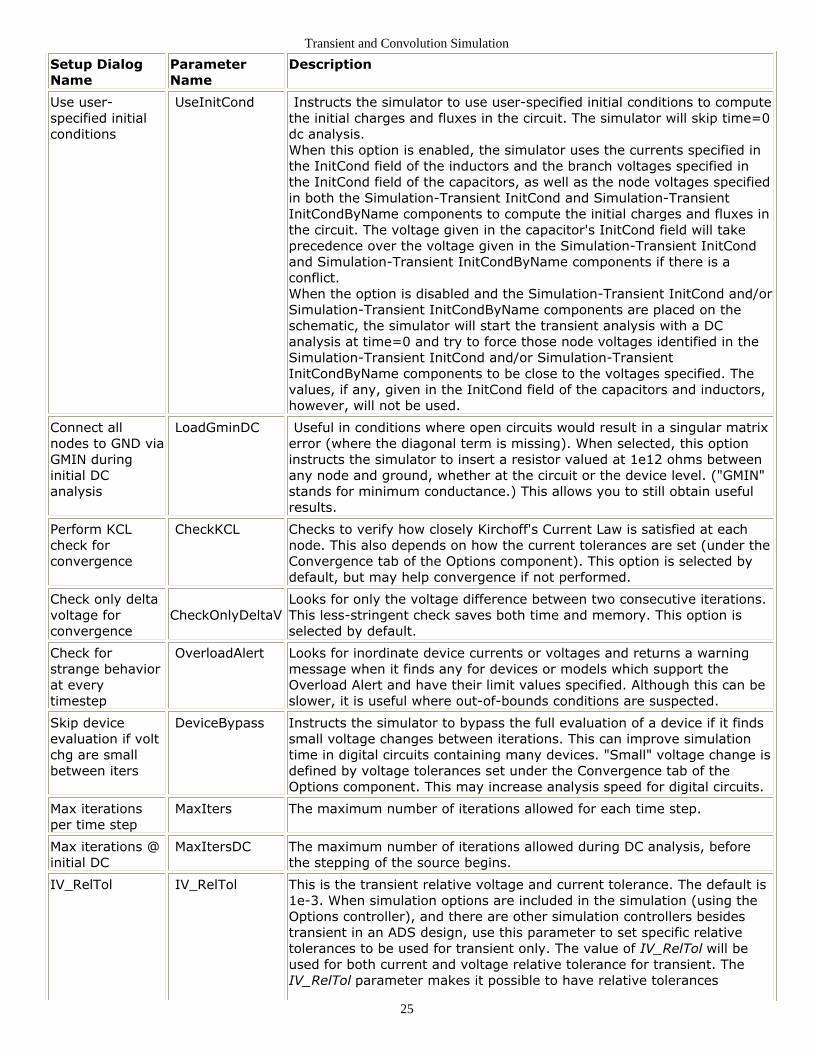
Use user-specified initialconditions

UseInitCond Instructs the simulator to use user-specified initial conditions to computethe initial charges and fluxes in the circuit. The simulator will skip time=0dc analysis.When this option is enabled, the simulator uses the currents specified inthe InitCond field of the inductors and the branch voltages specified inthe InitCond field of the capacitors, as well as the node voltages specifiedin both the Simulation-Transient InitCond and Simulation-TransientInitCondByName components to compute the initial charges and fluxes inthe circuit. The voltage given in the capacitor's InitCond field will takeprecedence over the voltage given in the Simulation-Transient InitCondand Simulation-Transient InitCondByName components if there is aconflict.When the option is disabled and the Simulation-Transient InitCond and/orSimulation-Transient InitCondByName components are placed on theschematic, the simulator will start the transient analysis with a DCanalysis at time=0 and try to force those node voltages identified in theSimulation-Transient InitCond and/or Simulation-TransientInitCondByName components to be close to the voltages specified. Thevalues, if any, given in the InitCond field of the capacitors and inductors,however, will not be used.

Connect allnodes to GND viaGMIN duringinitial DCanalysis

LoadGminDC Useful in conditions where open circuits would result in a singular matrixerror (where the diagonal term is missing). When selected, this optioninstructs the simulator to insert a resistor valued at 1e12 ohms betweenany node and ground, whether at the circuit or the device level. ("GMIN"stands for minimum conductance.) This allows you to still obtain usefulresults.

Perform KCLcheck forconvergence

CheckKCL Checks to verify how closely Kirchoff's Current Law is satisfied at eachnode. This also depends on how the current tolerances are set (under theConvergence tab of the Options component). This option is selected bydefault, but may help convergence if not performed.

Check only deltavoltage forconvergence

CheckOnlyDeltaV

Looks for only the voltage difference between two consecutive iterations.This less-stringent check saves both time and memory. This option isselected by default.

Check forstrange behaviorat everytimestep

OverloadAlert Looks for inordinate device currents or voltages and returns a warningmessage when it finds any for devices or models which support theOverload Alert and have their limit values specified. Although this can beslower, it is useful where out-of-bounds conditions are suspected.

Skip deviceevaluation if voltchg are smallbetween iters

DeviceBypass Instructs the simulator to bypass the full evaluation of a device if it findssmall voltage changes between iterations. This can improve simulationtime in digital circuits containing many devices. "Small" voltage change isdefined by voltage tolerances set under the Convergence tab of theOptions component. This may increase analysis speed for digital circuits.

Max iterationsper time step

MaxIters The maximum number of iterations allowed for each time step.

Max iterations @initial DC

MaxItersDC The maximum number of iterations allowed during DC analysis, beforethe stepping of the source begins.

IV_RelTol IV_RelTol This is the transient relative voltage and current tolerance. The default is1e-3. When simulation options are included in the simulation (using theOptions controller), and there are other simulation controllers besidestransient in an ADS design, use this parameter to set specific relativetolerances to be used for transient only. The value of IV_RelTol will beused for both current and voltage relative tolerance for transient. TheIV_RelTol parameter makes it possible to have relative tolerances


26

specifically for transient.

Setting Up Optional Parameters

Following is information on setting up the Tran Options portion of the simulation. Thefollowing table describes the parameter details. Names listed in the Parameter Namecolumn are used in netlists and on schematics.

Transient Simulation Options

SetupDialogName

ParameterName

Description

Levels Select the degree of simulation information to be reported.

Statuslevel

StatusLevel Prints information about the simulation in the Status/Summary part of theMessage Window.- 0 reports little or no information, depending on the simulation engine.- 1 and 2 yield more detail.- Use 3 and 4 sparingly since they increase process size and simulation timesconsiderably.The type of information printed may include the sum of the current errors ateach circuit node, whether convergence is achieved, resource usage, andwhere the dataset is saved. The amount and type of information depends onthe status level value and the type of simulation.

Deviceoperatingpoint level

DevOpPtLevel Enables you to save all the device operating-point information to the dataset. Ifthis simulation performs more than one Transient analysis (from multipleTransient controllers), the device operating point data for all Transient analyseswill be saved, not just the last one. Default setting is None.

None None No information is saved.

Brief Brief Saves device currents, power, and some linearized device parameters.

Detailed Detailed Saves the operating point values which include the device's currents, power,voltages, and linearized device parameters.

Output solutions

Output allinternaltime points

OutputAllPoints Causes the simulator to save simulation results at all internal timepoints; thisoption is on by default. Deselecting this option causes results to be saved atleast as often as the Max timestep option but some of the intermediate pointswill be suppressed. For simulations that take many small timesteps due toautomatic timestep control, but whose output is still well-sampled at Maxtimestep, this can make the resulting datasets smaller and make the post-processing of the data faster.

Defining the Noise Parameters

Following is information on setting up the Tran Noise portion of the simulation. Thefollowing table describes the parameter details. Names listed in the Parameter Namecolumn are used in netlists and on schematics.


27

Transient Simulation Noise Parameters

SetupDialogName

ParameterName

Description

Noisebandwidth

NoiseBandwidth Enables the generation of pseudorandom noise at each timestep.NoiseBandwidth controls the bandwidth of the generated noise and must beless than or equal to 1/(2*MaxTimeStep). If this parameter is not specified oris zero, no noise is generated.

Noise scale NoiseScale A multiplicative scaling applied to all generated noise.

Setting the Fundamental Frequencies

Following is information on setting up the frequency portion of the simulation. Thefollowing table describes the parameter details. Names listed in the Parameter Namecolumn are used in netlists and on schematics.

Transient Simulation Frequency Parameters


28

SetupDialogName

ParameterName

Description

Fundamental Frequencies

Edit Edit the Frequency and Order fields, then click Add to add the frequency to thelist in the Select area.

Frequency Freq[n] The frequency of the fundamental(s). Change value by typing over the entry inthe field. Select the units (None, Hz, kHz, MHz, GHz) from the drop-down list.

Order Order[n] The maximum order (harmonic number) of the fundamental(s) that will beconsidered. Change value by typing over the entry in the field.

Select Contains the list of fundamental frequencies and their orders. Use the Edit areato add fundamental frequencies to this window.- Add - Adds a frequency to the list.- Cut - Removes selected frequency from the list.- Paste - Enables you to move an item cut from the list to a new position.

Maximummixingorder

MaxOrder Determines how many mixing products are to be transformed for the multi-toneharmonic balance simulation. A mixing term, or mixing product, is a combinationof two or more fundamentals or their successive harmonics. Mixing products willoccur when there are multiple frequencies in a circuit.For example, consider having a simulation with Freq[1]=f1, Order[1]=4,Freq[2]=f2, Order[2]=5, and MaxOrder=3. The mixing products that are to betransformed are f1-f2, 2f1-f2, f1-2f2, f1+f2, 2f1+f2, and f1+2f2.If Maximum order is 0 or 1, no mixing products are simulated. If the MaxOrder isnot given, then it will be set to the largest order of the fundamental.

Compute HB Solution

Write InitialGuess forHB

HB_Sol Check this box to generate a transient initial guess for a harmonic balancesimulation.

File HB_OutFile Enter the name of the file for the transient initial guess. Be sure to use the filename when running the harmonic balance simulation. If no file name is entered(and Write Initial Guess for HB has been selected), then the name of the designwill be used as the default name.

ApplyWindow

HB_Window Applies a window to the time domain data. This window helps to minimize thespectral leakage when multiple frequency tones are present. The window type isa Blackman window. For multi-tone applications, it is recommended to enablethe Apply Window option.

Detect steadystate

SteadyState When enabled, causes the transient simulator to determine if the circuit reachessteady state. If steady state is reached, then the time value and frequency ofoscillation (if simulating an oscillator) will be reported. At least one frequencyand order pair (Freq[1] and Order[1]) must be specified when selecting thisparameter. For a transient assisted harmonic balance simulation, enableSteadyState for the simulator to generate a transient initial guess (whichcaptures the steady state portion of the waveform) for later use in the harmonicbalance simulation. The simulator will stop when a steady state has beenreached and transform just the last period of the solution. Thus, the transientsimulation may end earlier than the StopTime when steady state is reached.


29

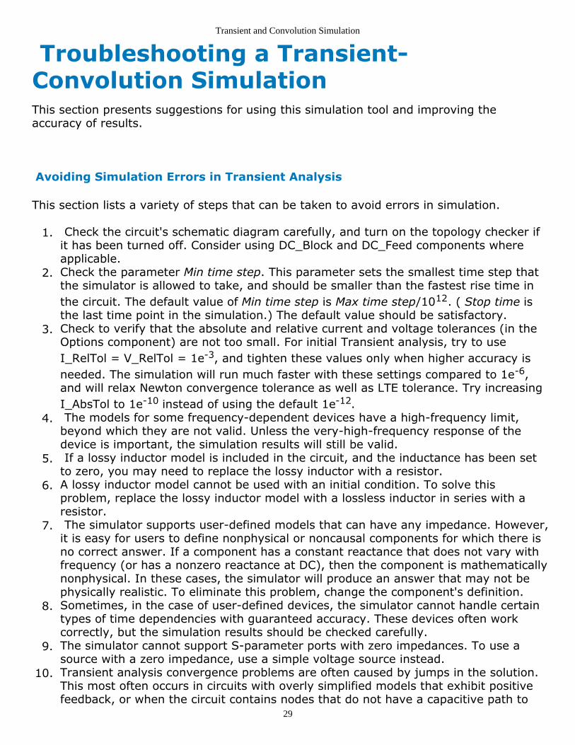
Troubleshooting a Transient-Convolution SimulationThis section presents suggestions for using this simulation tool and improving theaccuracy of results.

Avoiding Simulation Errors in Transient Analysis

This section lists a variety of steps that can be taken to avoid errors in simulation.

Check the circuit's schematic diagram carefully, and turn on the topology checker if1.it has been turned off. Consider using DC_Block and DC_Feed components whereapplicable.Check the parameter Min time step. This parameter sets the smallest time step that2.the simulator is allowed to take, and should be smaller than the fastest rise time inthe circuit. The default value of Min time step is Max time step/1012. ( Stop time isthe last time point in the simulation.) The default value should be satisfactory.Check to verify that the absolute and relative current and voltage tolerances (in the3.Options component) are not too small. For initial Transient analysis, try to useI_RelTol = V_RelTol = 1e-3, and tighten these values only when higher accuracy isneeded. The simulation will run much faster with these settings compared to 1e-6,and will relax Newton convergence tolerance as well as LTE tolerance. Try increasingI_AbsTol to 1e-10 instead of using the default 1e-12. The models for some frequency-dependent devices have a high-frequency limit,4.beyond which they are not valid. Unless the very-high-frequency response of thedevice is important, the simulation results will still be valid. If a lossy inductor model is included in the circuit, and the inductance has been set5.to zero, you may need to replace the lossy inductor with a resistor.A lossy inductor model cannot be used with an initial condition. To solve this6.problem, replace the lossy inductor model with a lossless inductor in series with aresistor. The simulator supports user-defined models that can have any impedance. However,7.it is easy for users to define nonphysical or noncausal components for which there isno correct answer. If a component has a constant reactance that does not vary withfrequency (or has a nonzero reactance at DC), then the component is mathematicallynonphysical. In these cases, the simulator will produce an answer that may not bephysically realistic. To eliminate this problem, change the component's definition.Sometimes, in the case of user-defined devices, the simulator cannot handle certain8.types of time dependencies with guaranteed accuracy. These devices often workcorrectly, but the simulation results should be checked carefully.The simulator cannot support S-parameter ports with zero impedances. To use a9.source with a zero impedance, use a simple voltage source instead.Transient analysis convergence problems are often caused by jumps in the solution.10.This most often occurs in circuits with overly simplified models that exhibit positivefeedback, or when the circuit contains nodes that do not have a capacitive path to


30

ground. Add a small capacitor from the troublesome node to ground and give acomplete capacitance model when specifying the nonlinear device model parameters.Generally analog circuits are sensitive to truncation error due to their relative long11.time constants. Use LTE time step control to ensure the accuracy of the results. Alsotry relaxing TruncTol by increasing this value to 10 times or more to relax LTEtolerance.Try different integration methods. Backward Euler (Gear1 or Mu=0 in Trapezoidal)12.and Gear2 are stable for all stable and some unstable differential equations.However, trapezoidal rule are stable only on stable differential equations. Switch toGear1 or Gear2 when trapezoidal rule fails on unstable differential equations. Add break points. Use piecewise linear source to add break points to the region13.where the waveform changes abruptly.

Solving Convergence Problems

Nonconvergence is a numerical problem encountered by the simulator when it cannotreach a solution, within a given tolerance, after a given number of iterations.

There is no single solution for solving convergence problems in transient and convolutionanalysis. Several ways to approach those problems are listed below.

Make sure that you have specified an appropriate value for Max time step. Reducethis value if necessary to ensure enough time points for sharp edges.Vary Integration coefficient mu in the case of high-Q circuits.Increase the time-point iteration limit, Max iterations per time step. Increase thisvalue to 50 or more to increase the possible number of Newton iterations on eachtime step.If the circuit includes a GaAsFET , reduce the value of the transit time TAU in thedevice model itself.Adjust the current and voltage relative and absolute tolerances in the Optionscomponent. Note the following guidelines:The relative tolerance parameters have a greater effect on simulation speed andaccuracy than the absolute tolerance parameters.Each order-of-magnitude change in accuracy (for example, from 10-3 to 10-4) willresult in approximately three times as many time points in the simulation.

Typical Convergence Problems

If you can attribute nonconvergence to any of the following areas, try these tips:

Capacitor model problems:

Use simplified device models that do not include capacitance model or incompletecapacitance model give a complete capacitance model when specifying nonlineardevice model parameters, in junction capacitance, include both depletion (at least)


31

and diffusion capacitances.Discontinuous jumps in waveforms when circuit contains nodes have no capacitivepath to ground add small capacitor to ground or specify Cmin.Capacitance model does not conserve charge GaAsFET Statz's, MOSFET Meyer'scapacitance models switch to charge based model.Large floating capacitors that are similar to the small-floating resistor problem in DC(finite precision problem) check capacitance unit, use smaller capacitance.Discontinuous capacitance models in user defined model, SDD device fix the model.

Slow Transient analysis:

Make sure I_RelTol and V_RelTol are set to 1e-3 or not set at all.Decrease these values when higher accuracy is needed.

Oscillator circuit does not oscillate:

Apply a short pulse at the beginning of the simulation.Avoid using Gear2 or backward Euler.

Circuit exhibits ringing or divergence:

Reduce Mu value from 0.5 toward 0 if trapezoidal rule is used.Use Gear1 or Gear2.

Circuit does not converge at first time point:

Reduce Min time step.

Avoiding Simulation Errors in Convolution Analysis

This section lists a variety of tips that can be used to avoid errors in simulation.

Using Convolution:

Don't set any convolution parameters (let the adaptive algorithm figure it out).Set ImpMaxFreq first (larger than signal bandwidth).Set convolution parameters on component, not controller, when possible.Don't allowed measured data to be extrapolated (either set ImpMaxFreq or providemore data).

Convolution Modeling for Time-Domain Simulation:

In time-domain simulation, simulate devices that can only be defined in thefrequency domain:

Transmission lines with dispersionDevices with frequency-dependent lossMeasured frequency-domain data


32

Convolution is the keyInverse Fourier transform of frequency-domain data produces the impulseresponse h(t)The impulse response is convolved with time-domain signal

Time and Frequency Range:

Impulse response is computed from the inverse Fourier transform of frequency-domain response. Frequency is uniformly sampled from 0 to some upper value.Upper frequency sets the time-domain spacing of the impulse responseFrequency spacing sets the length of the impulse response

Adaptive Impulse Response Calculation:

Estimate of system bandwidth is made from source frequencies and rise times - initialguess at fmax.Build a trial impulse response with 32 timepoints - very coarse frequency spacing.Build a second impulse response with 64 timepoints - less coarse frequency spacing.Keep doubling the number of timepoints until a good impulse response is obtained -increase fmax, decrease Df.y11 and y12 may be sampled with different fmax and Df.Adaptive calculation is only done if ImpDeltaFreq is not specified - don't setImpDeltaFreq if you don't have to.

Good Impulse Responses:

Compare impulse responses with N and 2N points. The second impulse response istwice as long in time domain and has half the frequency spacing.An impulse is considered "good" when no appreciable energy is present in the secondhalf of the impulse response.If energy is present in the second half, implies either that the impulse is not longenough or it is noncausal.If not good, Controller keeps doubling the length.Controller also tries doubling the maximum frequency, giving smaller impulsetimesteps.

Interpolation:

The impulse response is sampled with a uniform timestep, but is not guaranteed tomatch the simulation timestep. The simulation may even be using a variabletimestep.


33

Interpolate the signal v(t) to match the timepoints in the impulse response.Don't interpolate the impulse response because the Fourier transform of theinterpolated impulse response would no longer match the original frequencyresponse.

Impulse Evaluation:

Signal response at time zero extends back to minus infinity.Evaluate the integral as a sum.

Solving an Invalid Impulse Response

This is the most commonly encountered problem during convolution. It does notnecessarily imply noncausality but means that significant energy is present in the secondhalf of the impulse response. In addition, simulation results may or may not be valid.

Set ImpMaxFreq or ImpDeltaFreq. Set ImpMaxFreq first, typically only for measureddata.For every component that generates this message, fix each component one at a timeto simplify the design.

Viewing an Impulse Response


34

In an S-parameter simulation, analyze over the given frequency spacing andmaximum frequency - inverse Fourier transform the response by plotting ts(x) .In the time domain, apply an impulse and simulate plot the transient result - thepulse rise time is used to set fmax and thus can influence the impulse response.

Setting ImpMaxFreq and ImpDeltaFreq

Generally a good impulse response can be found without manually setting ImpMaxFreqand ImpDeltaFreq.

If ImpMaxFreq is set, the adaptive algorithm tries different lengths but doesn'tmodify fmax.If ImpDeltaFreq is set, the adaptive algorithm is disabled and the impulse iscomputed from ImpDeltaFreq and ImpMaxFreq.Set ImpMaxFreq on the component, then set ImpDeltaFreq on component ifnecessary, and finally, set ImpMaxFreq on the transient controller if necessary.For transmission lines, set ImpMaxFreq to at least n/td, where td is the delay timeand n is a small integer (2-3).For lowpass and bandpass filters, set ImpMaxFreq to at least twice the upperpassband edge.

Measured Data with S2P Component

The algorithm that computes the impulse response has no special knowledge of thecomponent it's working on and assumes data is available at any desired frequency. Ithas no knowledge of:

flow and fhigh of measured data

frequency spacing of measured dataS2P interpolates and extrapolates data as needed.Be sure to supply good data to prevent dangerous extrapolation extends down to DCand up to fmax.

Set ImpMaxFreq on S2P component to match frequency limits in datafile (avoidextrapolation).Typically there is not enough frequency-domain data in the S2P file for use in thesimulation.

Given a pulse with a rise time of tr, the equivalent bandwidth in Hertz is 0.35/tr(0.1 ns rise time represents a 3.5 GHz bandwidth).Package models typically must be measured up to 10x higher than the signalfrequency to represent transmission line effects well.

Solving a Noncausal Impulse Response


35

This is the second most commonly encountered problem during convolution. The Time-domain simulation starts at time zero and moves forward in time, computing the value ofnext timepoint from all previous timepoints. And the Controller deals with this byintroducing a delay to force causality. Length of delay set to ImpNoncausalLength(default=32) with timestep set by default ImpMaxFreq.

Simulation results will not be accurate because of the added delay, especially if the delayis added in a critical timing or phase path.

All physically realizable devices are causal (the output is dependent only on past statesand not any future states) while noncausal devices are nonphysical. Some ADScomponents, user-defined data or equations may be noncausal.

Frequency-dependent real part with constant imaginary part, for example resistanceas a function of frequency without any reactance.Constant real and constant non-zero imaginary part.Negative time delays.INDQ, CAPQ, PLCQ, SLCQ have problems in some modes.

Comparing Time-Domain and Steady-State Results

Certain circuit elements such as microstrip, discontinuities, and so on, are represented bysimplified models in a transient analysis. A few planar discontinuities are also treated asideal short or open circuits. Therefore, results from transient or convolution simulationmay differ from those for steady-state simulation on the same circuit, depending upon thetypes of elements used in the circuit. (A convolution simulation should yield results closerto those of a steady-state simulation.)

The frequency of operation also plays a major role. At low frequencies, simplified modelsor short-circuits may be valid approximations for certain dispersive models.

Setting Max Frequency and Other Convolution Parameters

In general, the synthesized impulse response accurately represents the frequency domainfunction over the frequency range specified by the convolution control parameter MaxFrequency. The simulation techniques require negligible spectral energy outside thisfrequency range. An accurate solution is not guaranteed if this principle is not obeyed.Therefore, setting Max Frequency correctly is the most important aspect of any transientsimulation using convolution-based devices.

Max Frequency is similar to choosing the number of harmonics in a harmonic balancesimulation or a time step in SPICE. In these cases you must estimate the value of theparameter prior to the simulation. Examination of the results reveals whether theparameter was chosen correctly. The built-in estimation of Max Frequency is always agood starting point.


36

The remaining convolution-control parameters described below are best used with theirdefault values for any causal device, such as a microstrip transmission line.

The Discrete convolution mode option, by causing a periodic extension of the frequencyresponse, generally leads to the most accurate and efficient description of the device fromDC to Max Frequency. Provided Max Frequency is set correctly, the frequency responsebeyond Max Frequency is irrelevant, because no significant spectral energy exists beyondthis value. The PWL Continuous option always leads to a low-pass response (which may bedesirable in cases where a low-pass response is being modeled). The discrete mode ismany times faster than the continuous mode.

Delta frequency defines the frequency spacing with which the convolution-based devicesare sampled in the frequency domain. If Delta frequency is not specified, the simulatoradaptively samples the frequency function until an appropriate value is determined. If youare unsure about the correct value of Delta frequency, simply allow the simulator todecide.

Non-causal fcn imp response length adjusts the length of the impulse responseassociated with the treatment of noncausal frequency responses (see discussion below).

Smoothing window type specifies the smoothing window to be applied to the time-domain impulse responses that are derived from noncausal frequency functions (such asHilbert transforms). The window reduces ripple in the approximation caused bydiscontinuities in the frequency function. (Refer to Dealing with Noncausal FrequencyResponses". (cktsimtrans))

Max impulse sample points places an upper limit on the allowed impulse-responselength. It is mainly used when Max Frequency is specified but Delta Frequency is not. It isnecessary to increase this value (default = 4096) if you specify a frequency response thatrequires a long impulse response.

Relative impulse truncation factor and Absolute impulse truncation factor areused to remove redundancy from the impulse responses. Setting them to a small valueleads to longer impulse responses and a more accurate description of the frequencyresponse of a convolution-based device. The simulator uses them to make decisions aboutthe relative sizes of individual members of an impulse response.

Dealing with Noncausal Frequency Responses

A causal system has the property that if the input is zero for t < t1, then the output is also

zero for t < t1. The value of t1 is usually defined to be 0. Therefore, the impulse response

of a causal system is zero for negative time. This may be stated in the frequency domainby saying that the real and imaginary parts of a causal frequency response are related bythe Hilbert transform: the Kramers-Kronig relation. Only causal frequency-domain transferfunctions can be handled directly by means of transient simulation methods.


37

However, there are many ideal frequency functions that are noncausal but are extremelyvaluable in processing signals (such as Hilbert transforms). The transient simulatorprovides a way to use these functions in defining the frequency response of a nonlineardevice.

A frequency response is considered noncausal if it has one of the following forms:

R + jIR(w) + j0R + jI(w)

When you select Non-causal fcn imp response length, non-causal frequency functions areapproximated by a digital filter that introduces a time delay in the impulse response. Thistime delay is sufficient to make the apparent impulse response causal. Non-causal fcn impresponse length defines the length of this filter. The Smoothing window type can beselected to reduce Gibb's phenomenon, which may be present if the non-causal frequencyresponse contains discontinuities. Increasing non-causal leads to a more accuratedescription of the frequency function over the chosen band set by Max Frequency.However, increasing non-causal causes a longer delay through the filter and a longersimulation time. Only even values of non-causal are allowed. If an odd value is specified,the simulator adds 1 and issues a warning. The delay associated with the causalapproximation is given by the equation: (noncausal/2-1)/(2*max Frequency).

If a non-causal frequency response is specified which does not fit into one of the formsdescribed above, the simulator will assume it is a causal function. This will almostcertainly cause unexpected and erroneous results. Noncausal frequency responses shouldbe avoided if possible.

The concept of causality is not an issue when using the harmonic balance simulator. Allexcitations and responses are sums of sinusoids and exist for all time. For this reason, anybounded frequency response can be simulated. When moving from harmonic balance totransient simulation, it must be remembered that non-causal frequency functions cannotbe simulated directly. Only a band-limited approximation to these functions can besimulated. This is particularly important when using SDD weighting functions.

Using Measured and Simulated S-Parameter Data

The ability to handle convolution-based devices allows the user of measured or simulatedS-parameter data to describe a wide variety of devices and circuits. A dataset or filecontaining the S-parameter values can be used to integrate the frequency response into atime-domain simulation. This adds a tremendous amount of flexibility to the number andtypes of devices and circuits which can be used in a simulation.

When S-parameter data is used, it is important that the frequency response be adequatelysampled over the entire bandwidth to ensure negligible interpolation errors when theimpulse response is being calculated. The Max Frequency parameter should never be setto a value which is greater that the maximum S-parameter data frequency. doing so will


38

lead to erroneous results as the available data would have to be extrapolated. S-parameter data must also extend all the way down to DC.

Documents

Transient and Convolution Simulationedadownload.software.keysight.com/eedl/ads/2011/pdf/cktsimtrans.pdf · Transient and Convolution Simulation 1 Advanced Design System 2011 ... HiSIM2