Embed Size (px)
Citation preview
Journal of The Electrochemical Society, 149 ~8! G461-G473~2002!0013-4651/2002/149~8!/G461/13/$7.00 © The Electrochemical Society, Inc.
G461
Transient Adsorption and Desorption in Micrometer ScaleFeaturesMatthias K. Gobbert, a,* ,z Samuel G. Webster,a and Timothy S. Caleb,*aDepartment of Mathematics and Statistics, University of Maryland, Baltimore County, Baltimore,Maryland 21250, USAbFocus Center-New York, Rensselaer: Interconnections for Gigascale Integration, Rensselaer PolytechnicInstitute, Troy, New York 12180-3590, USA
We present a Boltzmann equation-based model for transport and reaction in micrometer-scale features such as those found inintegrated circuit fabrication. We focus on the adsorption and desorption of one species to understand the transient responses tostep changes at the reactor scale. The transport model has no adjustable parameters; the assumptions are detailed. Adsorption anddesorption reactions and rates are written as simple reversible Langmuir rate expressions. Kinetic parameter values are chosen fordemonstration. Results for the transient behavior of number density, flux to the surface, and the surface coverage are related tothose that might occur during the adsorption and purge steps in an atomic layer deposition process. We conclude that forreasonable surface kinetics, the time scale for transport is much shorter than the time scale for adsorption and desorption and thatan analytical model provides reasonable estimates for processing times.© 2002 The Electrochemical Society.@DOI: 10.1149/1.1486452# All rights reserved.
Manuscript submitted August 3, 2001; revised manuscript received February 12, 2002. Available electronically June 17, 2002.
c ois, afeo
eoalhisnd
hiul
ionadeth
nn. Ttio
s
omthetrap
vefac, bals
alusch;
rear
hisfac
ee acus-di-
nu-dis-of aningandeen
-gastwo-cal
be
ys
ns
d
In an ideal atomic layer deposition~ALD ! process, the depositionof solid material on the substrate is accomplished one atomimolecular layer at a time, in a self-limiting fashion; this propertyresponsible for the recent interest in ALD. To accomplish thisrepresentative ALD process consists of repeating a sequence oactant flows and reactor purges. In the first step of a cycle, a gasspecies~A! is directed into the reactor, and~ideally! one monolayeradsorbs onto the surface. After purging the reactor, a second gasreactant~B! is directed through the reactor. A self-limiting chemicreaction forms the next layer of deposited film. By repeating tcycle of reactant flows and purges, a film of ideally uniform acontrolled thickness is deposited.1-4
Although ALD has the potential to deposit films of uniformthickness, to keep average rates at reasonably high levels,switching frequencies of reactants and purges are desired. A pfrequency that is too high may lead to nonuniform film depositon the feature scale, on the wafer scale, or both. As a start towunderstanding species transport in features during ALD, we mothe adsorption of species A and the desorption that occurs duringfollowing purge in one cycle of a ALD process. We use a Boltzmaequation-based transport model with no adjustable parameterschemical reaction model used for the adsorption and desorprates are those found in typical mechanistic representationsimple reversible Langmuir adsorption.
We consider the case in which the flux of reactive species frthe source volume to the wafer surface is constant with time, eiat zero or at some selected value. Essentially, we idealize thesients at the reactor scale, and focus on modeling feature scalecesses in response to these idealized steps in concentration abowafer surface. More general boundary conditions at the interbetween the wafer surface and the reactor volume are possiblethe results presented below provide considerable insight. Weassume that the process is isothermal in time and space.
For an introduction to a deterministic approach to feature sctransport and reaction modeling and simulation that has beenfor deposition and etch processes, see Ref. 5, 6. That approavalid for processes for which a pseudo-steady assumption holdsi.e.,for which changes on the feature scale are slow relative to thedistribution of fluxes in the feature. On the other hand, transientscentral to ALD, and we need to start with a transient model. In tpaper, we consider cases for which the fluxes to the wafer surare constant with time~with the exception of step changes!. For
* Electrochemical Society Active Member.z E-mail: [email protected]
r
re-us
us
ghse
rdle
henof
rn-ro-theeuto
eedis
-e
e
transients that are present on the time scale of processes, sdiscussion on programmed rate processing in Ref. 7. For a dission on the dimensionality of transport modeling relative to themensionality of surface representation, see Ref. 8.
We describe the model in the next section, then outline themerical approach in the following section. We then present andcuss some simulation results for the adsorption and purge stepsALD process. Preliminary results for adsorption without considerdesorption and with different choices of reference quantitieswith a less precise estimate for the equilibrium fluxes have bpresented.9
The Model
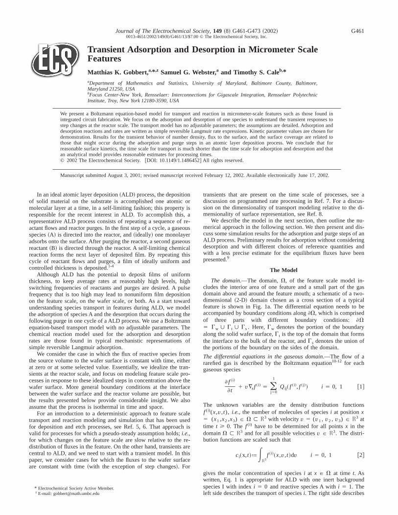
The domain.—The domain,V, of the feature scale model includes the interior area of one feature and a small part of thedomain above and around the feature mouth; a schematic of adimensional~2-D! domain chosen as a cross section of a typifeature is shown in Fig. 1a. The differential equation needs toaccompanied by boundary conditions along]V, which is comprisedof three parts with different boundary conditions:]V5 Gw ø G t ø Gs. Here,Gw denotes the portion of the boundaralong the solid wafer surface,G t is the top of the domain that formthe interface to the bulk of the reactor, andGs denotes the union ofthe portions of the boundary on the sides of the domain.
The differential equations in the gaseous domain.—The flow of ararefied gas is described by the Boltzmann equation10-12 for eachgaseous species
] f ~ i!
]t1 v¹xf ~ i! 5 (
j50
1
Qij~ f ~ i!, f ~ j!! i 5 0, 1 @1#
The unknown variables are the density distribution functiof (i)(x,v,t), i.e., the number of molecules of speciesi at positionx5 (x1 ,x2 ,x3) P V , R3 with velocity v 5 (v1 , v2 , v3) P R3 attime t > 0. The f (i) have to be determined for all pointsx in thedomainV , R3 and for all possible velocitiesv P R3. The distri-bution functions are scaled such that
ci~x,t !ªER3
f ~ i!~x,v,t !dv i 5 0, 1 @2#
gives the molar concentration of speciesi at x P V at time t. Aswritten, Eq. 1 is appropriate for ALD with one inert backgrounspecies I with indexi 5 0 and reactive species A withi 5 1. Theleft side describes the transport of speciesi. The right side describes
theofli-demu
ho
k-
sg
oati
l
ma
ax
th
lve
the
by
thesimi-
ure
thefor
r-
e-
Journal of The Electrochemical Society, 149 ~8! G461-G473~2002!G462
the effect of collisions among molecules of all species, in whichcollision operatorsQij model the collisions between moleculesspeciesi and j. The following paragraphs show how we treat colsional transport of reactive species in a background gas. Thisvation is important to arrive at the appropriate dimensionless forlation of the Boltzmann equation for free molecular flow.
Assuming that the reactive speciesj 5 1 is an order of magni-tude less concentrated than the background gas 0, it can be sthat it is justified to keep only the collision operatorsQi0 and neglectQi1 in every equationi 5 0, 1. If we also assume that the bacground gas is uniformly distributed in space (¹xf (0) 5 0), at equi-librium (] f (0)/]t 5 0), and inert~does not react with the speciej 5 1!, then the equation forf (0) is decoupled from the remaininone for the reactive species and consists in fact ofQ00( f (0), f (0))5 0 only, which has as a solution a Maxwellian10,11
f ~0!~x,v,t ! 5 M0ref~v !ª
c0ref
@2p~v0`!2#3/2 expS 2
uvu2
2~v0`!2D @3#
wherec0ref andv0
` denote a reference concentration and the thermdynamic average speed, respectively. The reference concentrcan be chosen from the ideal gas law as
c0ref 5
P0
RgT@4#
where the partial pressure of species 0 is given byP0 5 x0Ptotal
based on the given mole fractionx0 , andRg denotes the universagas constant; see Table I. The temperatureT in this paper is theconstant and spatially uniform temperature in Table I. The theraverage speed, which is used in the Maxwellian, is given by
v0` 5 AR0T 5 AkB
m0T 5 ARg
v0T @5#
based on the molecular weightv0 . The universal gas constantRg
and the universal Boltzmann constantkB are related throughAvogadro’s numberNA by Rg 5 NAkB ; see Table I. Writing(v0
`)2 5 R0T results in another common representation of the Mwellian
M0ref~v ! 5
c0ref
~2pR0T!3/2 expS 2uvu2
2R0TD @6#
Note that the Maxwellian is designed to have the same units asdensity functionsf (i).
Using the explicit solution for the background species, we sothe linear Boltzmann equation for the reactive species
Figure 1. ~a! Schematic of a two-dimensional domain defining lengthL andaspect ratioA. ~b! Numerical mesh for the feature withL 5 0.25 mm andaspect ratioA 5 4.
ri--
wn
-on
l
-
e
] f ~1!
]t1 v¹xf ~1! 5 Q1~ f ~1!! @7#
with the linear collision operatorQ1( f (1))ªQ10( f (1),M0ref). Notice
that decoupling from the background gas relied materially onassumption that it is an inert gas.
Define a reference Maxwellian also for the reactive species
M1ref~v ! 5
c1ref
@2p~v1`!2#3/2 expS 2
uvu2
2~v1`!2D @8#
wherec1ref and v1
` denote again a reference concentration andthermodynamic average speed for the species. They are chosenlarly as for the background species, see Table I.
The reference quantities for the nondimensionalization procedare listed in Table II. The reference concentrationc* and referencespeedv* are chosen equal to the corresponding quantities forreactive species. After defining the reference length appropriatethe domain size asL* 5 1 mm, we obtain on one hand the refeence time for transport fromt* 5 L* /v* . The mean free pathl isabout 100mm at the operating conditions listed in Table I and d
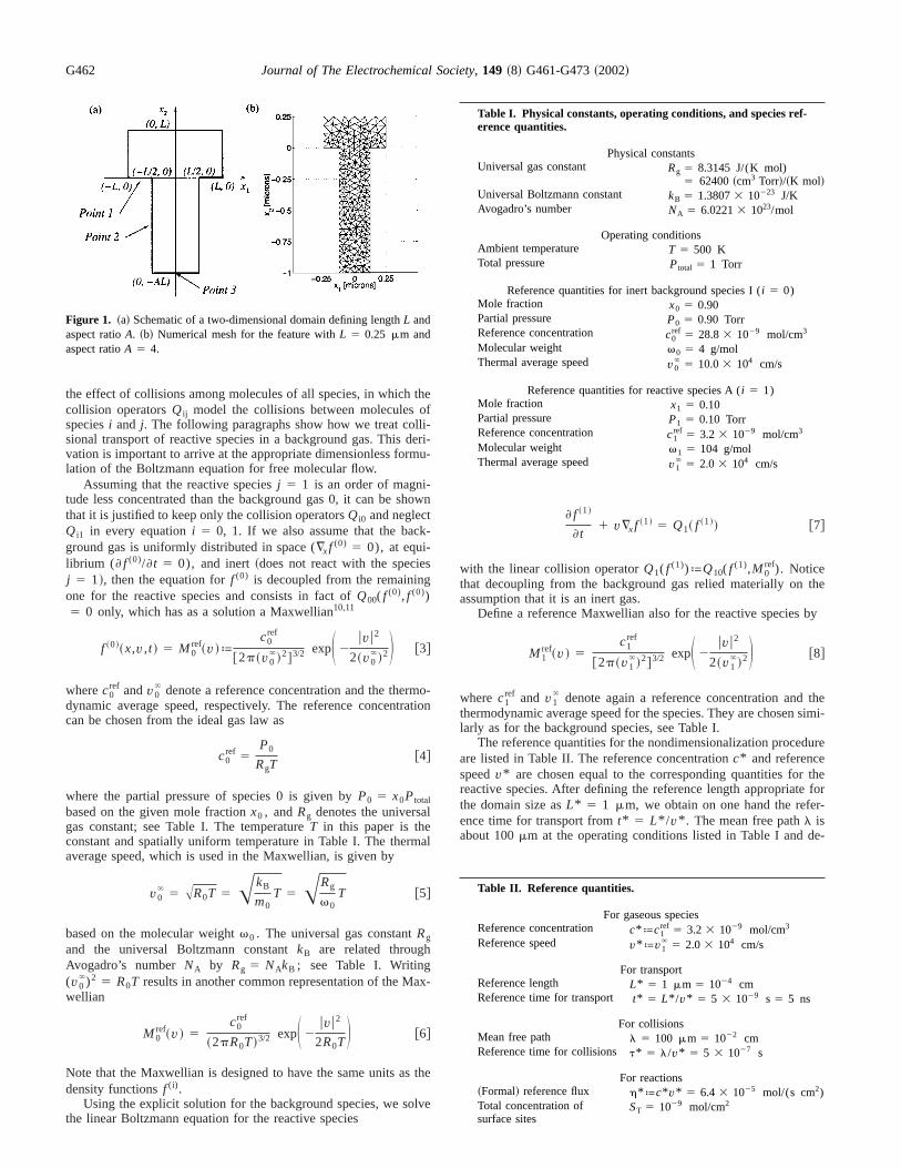
Table I. Physical constants, operating conditions, and species ref-erence quantities.
Physical constantsUniversal gas constant Rg 5 8.3145 J/(K mol)
5 62400~cm3 Torr!/~K mol!Universal Boltzmann constant kB 5 1.38073 10223 J/KAvogadro’s number NA 5 6.02213 1023/mol
Operating conditionsAmbient temperature T 5 500 KTotal pressure Ptotal 5 1 Torr
Reference quantities for inert background species I (i 5 0)Mole fraction x0 5 0.90Partial pressure P0 5 0.90 TorrReference concentration c0
ref 5 28.83 1029 mol/cm3
Molecular weight v0 5 4 g/molThermal average speed v0
` 5 10.03 104 cm/s
Reference quantities for reactive species A (i 5 1)Mole fraction x1 5 0.10Partial pressure P1 5 0.10 TorrReference concentration c1
ref 5 3.2 3 1029 mol/cm3
Molecular weight v1 5 104 g/molThermal average speed v1
` 5 2.0 3 104 cm/s
Table II. Reference quantities.
For gaseous speciesReference concentration c*ªc1
ref 5 3.2 3 1029 mol/cm3
Reference speed v*ªv1` 5 2.0 3 104 cm/s
For transportReference length L* 5 1 mm 5 1024 cmReference time for transport t* 5 L* /v* 5 5 3 1029 s 5 5 ns
For collisionsMean free path l 5 100 mm 5 1022 cmReference time for collisions t* 5 l/v* 5 5 3 1027 s
For reactions~Formal! reference flux h*ªc* v* 5 6.4 3 1025 mol/(s cm2)Total concentration ofsurface sites
ST 5 1029 mol/cm2
he
III
ucndhtre
olt
-
oranpr
andre-
po-n
ted
onby
ent
the
he
ov-
lu-
ffi-nioncifi-
Journal of The Electrochemical Society, 149 ~8! G461-G473~2002! G463
termines a reference time for collisions~the mean collision time! byt* 5 l/v* . The ratio of those times or lengths is equal to tKnudsen number Kn5 l/L* 5 t* /t* .
The choices of dimensionless variables are listed in TableThey result in the dimensionless Maxwellian
M1ref~ v ! 5
c1ref
@2p~ v1`!2#3/2 expS 2
uvu2
2~ v1`!2D @9#
where the dimensionless groupsc1ref and v1
` are included in TableIV. The dimensionless Boltzmann equation is obtained by introding the dimensionless variables in Table III. Notice that the left-haside is nondimensionalized with respect to transport, while the righand side is nondimensionalized with respect to collisions. Thissults in the Knudsen number appearing in the dimensionless Bmann equation for the reactive species
] f ~1!
] t1 v • ¹x f ~1! 5
1
KnQ1~ f ~1!! @10#
Since Kn for gaseous flow on the feature scale is large, Kn@ 1 ~seeTable IV!; we obtain the equation of free molecular flow
] f ~1!
] t1 v • ¹x f ~1! 5 0 @11#
The surface reaction model.—We model the adsorption of molecules of A as reversible adsorption on a single site13
A 1 vAv @12#
whereAv is adsorbed A, andv stands for a surface site available fadsorption. Although there are additional reaction steps for ALDother practical processes, this adsorption/desorption reaction
Table III. Dimensionless variables.
Time t 5t
t*
Lengths x 5x
L*
Velocities v 5vv*
, vi` 5
v i`
v*
Concentrations ci 5ci
c*, ci
ref 5ci
ref
c*
citop 5
citop
c*, ci
ini 5ci
ini
c*
Density distributions f ~ i! 5~v* !3
c*f ~ i!
f itop 5
~v* !3
c*fitop
f iini 5
~v* !3
c*f i
ini
Maxwellians M iref 5
~v* !3
c*M i
ref
Collision operators Qij 5~v* !3t*
c*Qij ,
Qi 5~v* !3t*
c*Qi
Fluxes, reaction rates h i 5h i
h*, R1 5
R1
h*
Fractional surface coverage qA 5SA
ST
.
-
--
z-
do-
vides a good vehicle through which to demonstrate our transportreaction modeling methodology, and it provides useful insightgarding modeling requirements.
The total molar concentration of surface sites available for desition is denoted byST , see Table II. IfSA denotes the concentratioof adsorbed molecules of A, the differenceST 2 SA is the concen-tration of vacant sites, and the reaction rate can be written as
R1 5 k1f ~ST 2 SA!h1 2 k1
bSA @13#
whereh1 denotes the flux of species to the surface, which is relato the distribution function of Eq. 1 by
h1~x,t ! 5 En • v8 . 0
un • v8u f ~1!~x,v8,t !dv8 x P Gw @14#
Here,Gw denotes the points at the wafer surface andn [ n(x) is theunit outward normal vector atx P Gw . Notice that the integral isover all velocities pointing out of the domain due to the conditin • v8 . 0. The evolution of the concentration of sites occupiedA at every point x at the wafer surfaceGw is given by
dSA~x,t !
dt5 R1~x,t ! x P Gw @15#
Notice that this model assumes that there is no significant movemof molecules along the surface.
If we nondimensionalize the reaction rate with respect toreference fluxh* and introduce the fractional surface coverageqA
5 SA /ST P @0,1#, we obtain the dimensionless reaction rate
R1 5 g1f ~1 2 qA!h1 2 g1
bqA @16#
with the dimensionless coefficients given in Table IV. Making tdifferential equation forSA dimensionless, we obtain
dqA~ x,t !
d t5 apR1~ x, t ! x P Gw @17#
with the prefactorap 5 (h* t* )/ST . This differential equation issupplied with an initial condition that represents the fractional cerageqA
ini at the initial time.Note that it is in general impossible to find a closed-form so
tion qA( t ) to the differential equation Eq. 17, because the coecients involvingh1 are not constant. But if this flux is constant, theEq. 17 becomes a first-order linear ordinary differential equatwith constant coefficients and can be solved analytically. Specally, at each point on the feature surface, we have the problem
dqA~ t !
d t5 2apbqA~ t ! 1 apg1
f h1 qA~0! 5 qAini @18#
Table IV. Dimensionless groups.
For species A (i 5 1)Dimensionless reference concentration c1
ref 5 1.0Dimensionless reference speed v1
` 5 1.0
For transport and collisionsKnudsen number Knªl/L* 5 100
For reactionsReaction coefficients for Reaction 1 g1
f 5 STk1f ,
g1b 5
ST
h*k1
b
Prefactor ap 5h* t*
ST5 0.323 1023
e-atio
mise
resth.
at
the
um-
ce
en-
darye-
by
fhe
iser-el
en-liza-ore
rtial
or
the
Journal of The Electrochemical Society, 149 ~8! G461-G473~2002!G464
with ap 5 (h* t* )/ST andb 5 g1f h1 1 g1
b , which has the solution
qA~ t ! 5 qA`~1 2 e2apbt ! 1 qA
inie2apbt @19#
with the equilibrium limit
qA` 5
g1f h1
g1f h1 1 g1
b @20#
provided thath1 is constant. Clearly,qA( t ) → qA` as t → `, hence
the name for the constantqA` . Note that this assumes that the sp
cies fluxes from the source above the wafer are constant. Equ
20 is also the solution of Eq. 16 withR1 set to zero~equilibrium!.
Boundary conditions for the Boltzmann equation.—At the wafersurface,Gw , we use the boundary condition
f ~1!~x,v,t ! 5 @h1~x,t ! 2 R1~x,t !#C1~x!M1ref~v !
n • v , 0 x P Gw @21#
whereh1 is the flux of species 1 to the surface andR1 is the reactionrate of Reaction 1. The boundary condition assumes diffusive esion of molecules,i.e., with the same velocity distribution as threference Maxwellian.10,12 In the absence of a reaction (R1 5 0),the inflowing part of f (1) is then proportional to the flux to thesurfaceh1 , because all molecules are being re-remitted. In the pence of a reaction though, the rate of reemission differs fromincoming flux by the reaction rateR1 , which could have either sign
The factorC1 is chosen as
C1~x! 5 S En • v,0
un • vuM1ref~v !dv D 21
@22#
to guarantee mass conservation in the absence of reactions, thwe require that influx equal to outflux forR1 5 0
En • v,0
un • vu f ~1!~x,v,t !dv 5 En • v.0
un • vu f ~1!~x,v,t !dv
@23#
Notice that C1(x) depends on the positionx P Gw via the unitoutward normal vectorn(x).
Using the reference fluxh* , formally chosen ash* 5 c* v*~see Table II!, the dimensionless boundary condition attainssame form as the dimensional one as
f ~1!~ x,v, t ! 5 @h1~ x, t ! 2 R1~ x, t !#C1~ x!M1ref~ v !
n • v , 0 x P Gw @24#
with the dimensionless flux to the surface
h1~ x, t ! 5 En • v8.0
un • v8u f ~1!~ x,v8, t !dv8 @25#
and with
C1~ x! 5 S En • v,0
un • vuM1ref~ v !dv D 21
@26#
The top of the domain of the feature scale modelG t forms theinterface to the bulk of the gas domain in the reactor, and we assthat the distribution off (1) is known there. More precisely, we assume that the inflow has a Maxwellian velocity distribution, hen
n
-
-e
is,
e
f ~1!~x,v,t ! 5 f 1topª
c1top
@2p~v1`!2#3/2 expS 2
uvu2
2~v1`!2D
n • v , 0 x P G t @27#
Using the dimensionless variables in Table III results in the dimsionless boundary condition
f ~1!~ x,v, t ! 5 f 1top 5
c1top
@2p~ v1`!2#3/2 expS 2
uvu2
2~ v1`!2D
n • v , 0 x P G t @28#
On the sides of the domainGs, which are perpendicular to themean wafer surface, we use specular reflection for the bouncondition to simulate an infinite domain. This condition can immdiately be stated in dimensionless form as
f ~1!~ x,v, t ! 5 f ~1!~ x,v8, t ! n • v , 0 x P Gs @29#
with
v8 5 v 2 2n~n • v ! @30#
Finally, we assume that the initial distribution of gas is given
f ~1!~x,v,t ! 5 f 1iniª
c1ini
@2p~v1`!2#3/2 expS 2
uvu2
2~v1`!2D
x P V t 5 0 @31#
with a Maxwellian velocity distribution; in particular, the choice oc1
ini 5 0 results in no gas of species 1 in the domain initially. Tdimensionless initial condition is then
f ~1!~ x,v, t ! 5 f 1ini 5
c1ini
@2p~ v1`!2#3/2 expS 2
uvu2
2~ v1`!2D
x P V t 5 0 @32#
If the reference concentration in the reference Maxwellianchosen asc1
ref 5 c1top and there are no surface reactions, the ref
ence Maxwellian will be the exact equilibrium solution of the modby construction.
Numerical
This paper reports on numerical results obtained in two dimsions, and the numerics are stated in 2-D form here; the generation to three dimensions is straightforward, but considerably mcomputationally intense. To simplify notation, the carets (• ) usedto indicate dimensionless variables are omitted in this section.
The solutionf (1)(x,v,t) to the kinetic equation Eq. 11 togethewith the boundary conditions Eq. 24, 28, and 29, and the inicondition Eq. 32 depends on xP V , R2, v P R2, and t > 0.Neglecting also the superscript off (1) in this section to simplifynotation, Eq. 11 forf (x,v,t) in two dimensions reads explicitly
] f
]t1 v ~1!
] f
]x11 v ~2!
] f
]x25 0 @33#
wherev (1) and v (2) denote the components of the velocity vectv 5 (v (1), v (2)) P R2 in the x1 andx2 directions, respectively.
We approach the problem by discretizing the components ofvelocity vector in Cartesian coordinates byvk1
(1) , k1 5 0, . . . , K1
2 1, in thev (1) variable and byvk2
(2) , k2 5 0, . . . , K2 2 1 in the
Journal of The Electrochemical Society, 149 ~8! G461-G473~2002! G465
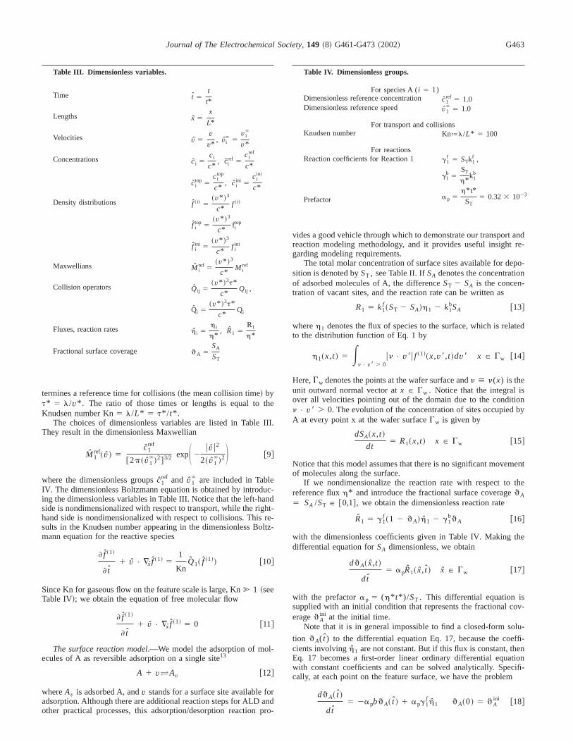
Figure 2. Adsorption step: dimensionless number density for a feature with aspect ratioA 5 4 for g1f 5 1.0 andg1
b 5 0.01 at times~a! 10.0 ns,~b! 40.0 ns,~c! 80.0 ns,~d! 1.0 ms,~e! 2.0 ms,~f! 3.0 ms. Note the different scales on thex1 and thex2 axes.
yf
v (2) variable. The velocity discretization is then defined byvk
5 (vk1
(1) ,vk2
(2)), k 5 0, . . . , K 2 1, with K 5 K1K2 , using the for-
mulask1 5 k 2 K1k2 andk2 5 bk/K1c.Now expand the unknownf for the reactive species in velocit
space
f ~x,v,t ! 5 (k50
K21
f k~x,t !wk~v ! @34#
where thewk(v), k 5 0, 1, . . . ,K 2 1, form an orthogonal set o
du
etha
o
ith
ith
Journal of The Electrochemical Society, 149 ~8! G461-G473~2002!G466
basis functions in velocity space with respect to some inner pro^ • , • &C , namely, ^wk ,wk&C 5 qk Þ 0 for all k and ^w l ,wk&C
5 0 for all l Þ k. Following ideas in Ref. 14, it is possible to maka judicious choice of basis functions such that it also holds^v (1)wk ,wk&C 5 qkvk1
(1) and^v (2)wk ,wk&C 5 qkvk2
(2) for all k as well
as ^v (1)w l ,wk&C 5 0 and^v (2)w l ,wk&C 5 0 for all l Þ k.To obtain an equivalent system of equations for the vector
coefficient functions
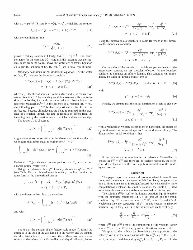
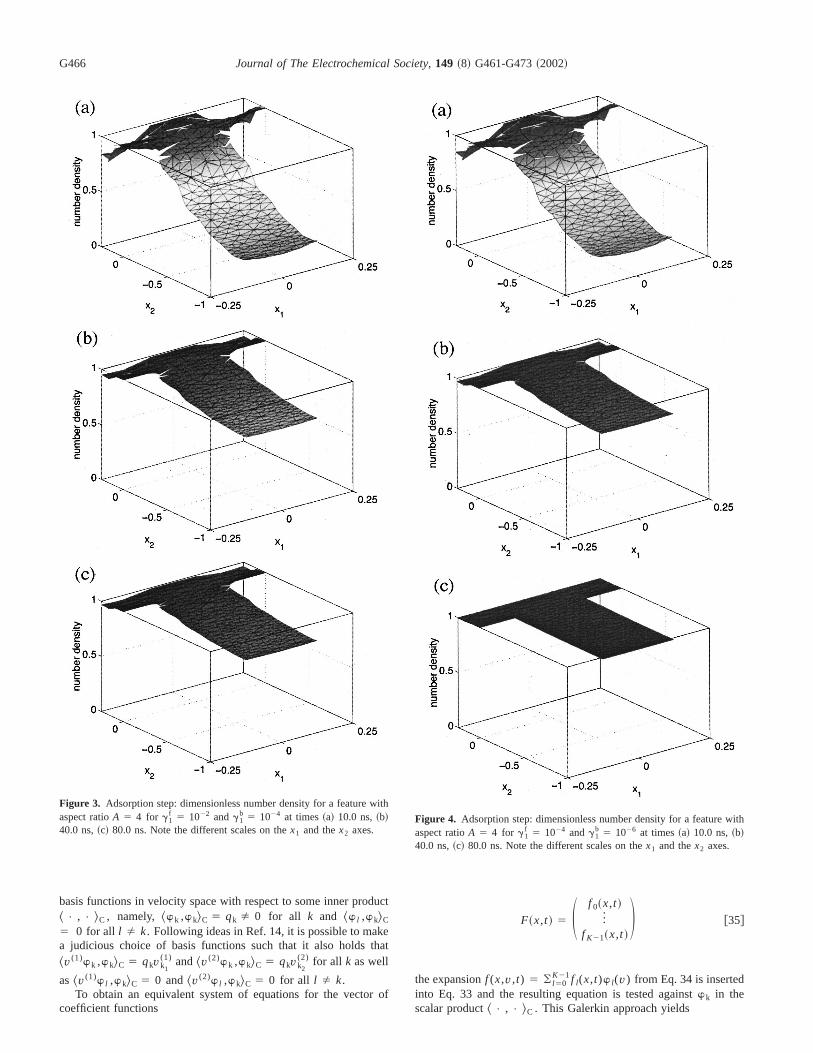
Figure 3. Adsorption step: dimensionless number density for a feature waspect ratioA 5 4 for g1
f 5 1022 andg1b 5 1024 at times~a! 10.0 ns,~b!
40.0 ns,~c! 80.0 ns. Note the different scales on thex1 and thex2 axes.
ct
t
f
F~x,t ! 5 S f 0~x,t !]
f K21~x,t !D @35#
the expansionf (x,v,t) 5 ( l 50K21f l(x,t)w l(v) from Eq. 34 is inserted
into Eq. 33 and the resulting equation is tested againstwk in thescalar product • , • &C . This Galerkin approach yields
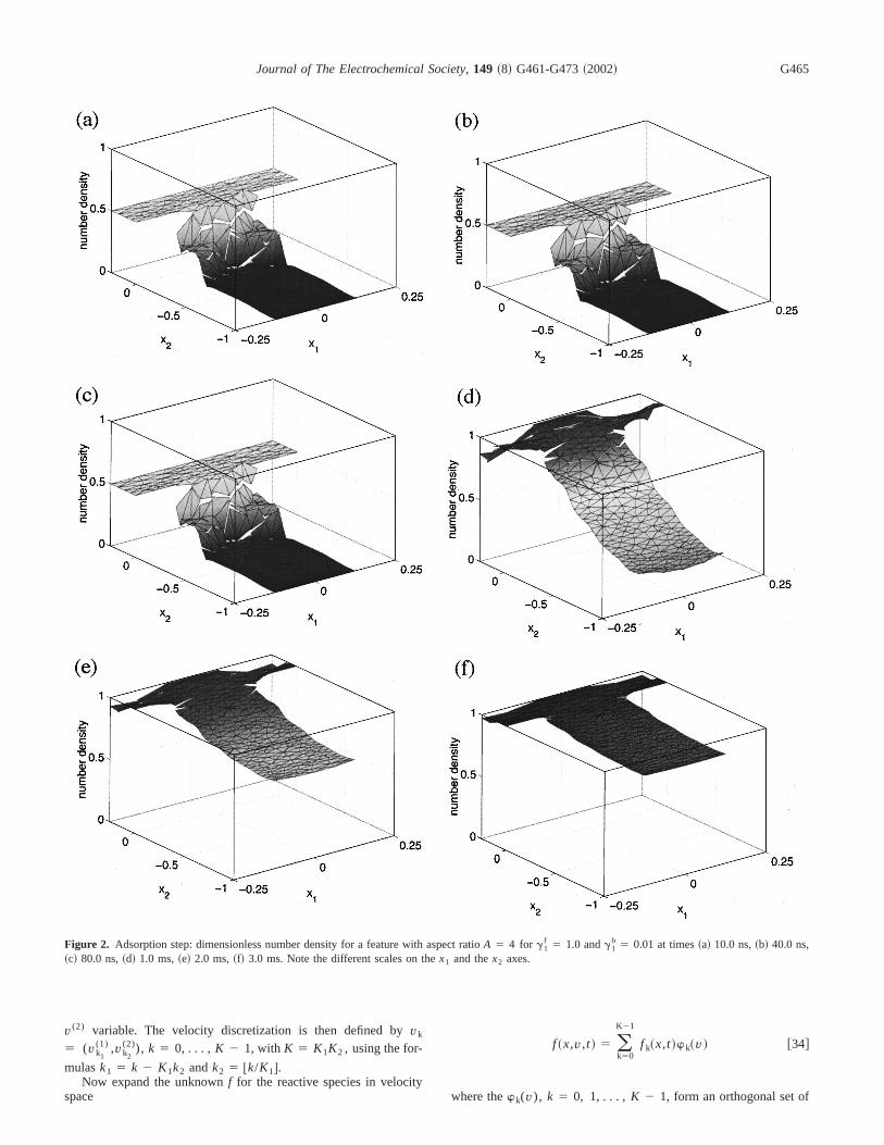
Figure 4. Adsorption step: dimensionless number density for a feature waspect ratioA 5 4 for g1
f 5 1024 andg1b 5 1026 at times~a! 10.0 ns,~b!
40.0 ns,~c! 80.0 ns. Note the different scales on thex1 and thex2 axes.
tem
-
cal
Journal of The Electrochemical Society, 149 ~8! G461-G473~2002! G467
(l 50
K21
^w l ,wk&C
] f l
]t1 (
l 50
K21
^v ~1!w l ,wk&C
] f l
]x1
1 (l 50
K21
^v ~2!w l ,wk&C
] f l
]x25 0 @36#
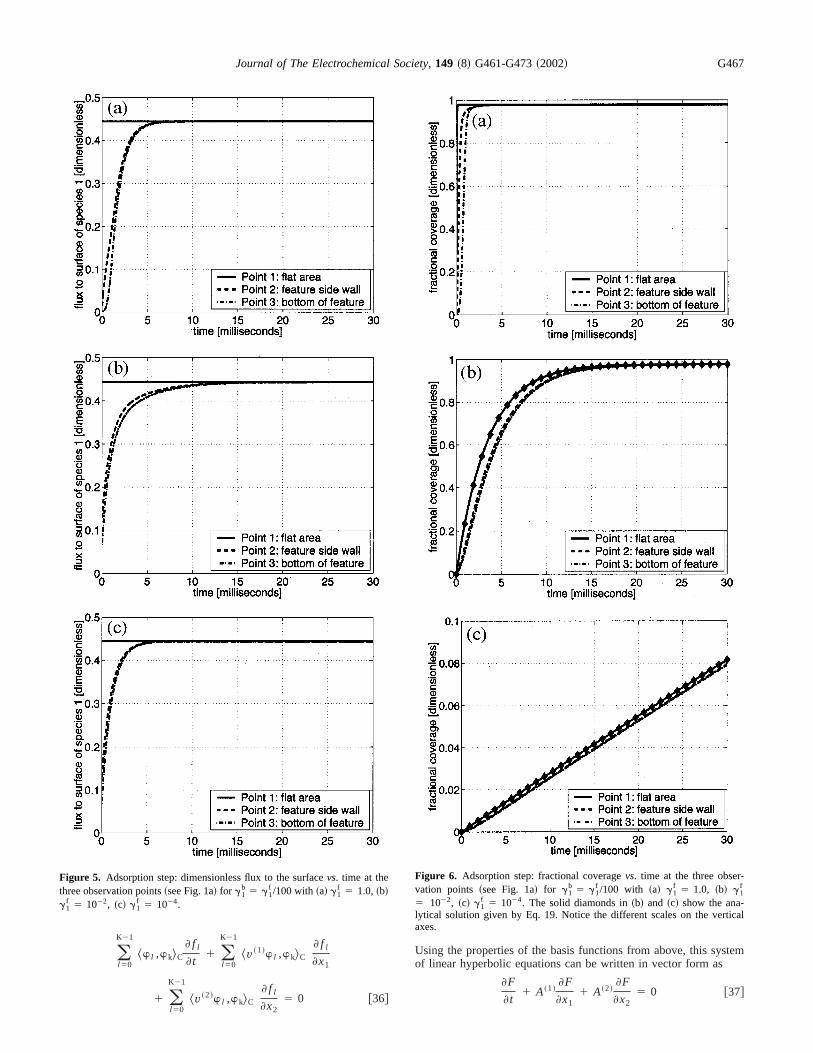
Figure 5. Adsorption step: dimensionless flux to the surfacevs. time at thethree observation points~see Fig. 1a! for g1
b 5 g1f /100 with~a! g1
f 5 1.0,~b!g1
f 5 1022, ~c! g1f 5 1024.
Using the properties of the basis functions from above, this sysof linear hyperbolic equations can be written in vector form as
]F
]t1 A~1!
]F
]x11 A~2!
]F
]x25 0 @37#
Figure 6. Adsorption step: fractional coveragevs. time at the three observation points ~see Fig. 1a! for g1
b 5 g1f /100 with ~a! g1
f 5 1.0, ~b! g1f
5 1022, ~c! g1f 5 1024. The solid diamonds in~b! and ~c! show the ana-
lytical solution given by Eq. 19. Notice the different scales on the vertiaxes.
n
tane tre-blehoeodut
disooatTh
theetionififor
rpThpr
V.
ee
etoptepns
d o
oin
ful
th
s.
no
of
urceonially
tofur-
thetion
triesse
in
rtfer
s and
leded asnorface
, it
akesface.nt
arlyon-ture
co-he
rfaces,
fi-
d 3
theuth.the4,ndsten
q.
Journal of The Electrochemical Society, 149 ~8! G461-G473~2002!G468
with diagonal matricesA(1), A(2) P RK3K that have the entriesAkk
(1) 5 vk1
(1) and Akk(2) 5 vk2
(2) . First mathematical results based othis approach can be found in Ref. 15, 16.
This system of linear hyperbolic equations is now posed in sdard form amenable for numerical computations. However, duits large sizeK, the irregular structure of the domain, and thequirement to compute for long times, it still poses a formidachallenge. It is solved using the discontinuous Galerkin metimplemented in the code DG,17 which is well-suited to the task. SeRef. 18, 19 for more detailed information on the numerical meth
The demonstration results presented in this paper are compusing four discrete velocities in eachx1 and x2 direction; hence,there areK 5 16 equations. Most results were checked againstcretizations using six discrete velocities in each direction, and gagreement was found for each of these comparisons. The spdomain was meshed coarsely to save on computation time.mesh for the domain is shown in Fig. 1b. As shown below,coarse mesh and the value ofK are sufficient to show that the timscale for transport is much faster than the time scale for adsorpfor reasonable adsorption chemistries. In turn, this leads to a sigcantly simpler model that has the analytical solution of Eq. 19the surface fractions.
Results
In this section, we report some simulation results for the adsotion step and the purge step that might be part of an ALD cycle.model is given by the dimensionless equations presented in thevious section. Some parameter values used are listed in Table Iaddition, we need to specify the~dimensionless! reaction parametersin Eq. 16; they are specified below. To complete the model, we nto choose the initial condition for the~dimensionless! gas concen-tration throughout the domainc1
ini and for the fractional coveragqA
ini , as well as the coefficient in the boundary condition at theof the domainc1
top; these values are different for the adsorption sand the purge step, and are specified in the following subsectio
In order to analyze the behavior of the fluxh1 to the surface andof the fractional surface coverageqA over time, three points on thewafer surface are chosen as shown in Fig. 1a. Point 1 is locatethe flat area of the wafer surface at (20.75L,0); during adsorption,we expect the fractional coverage to increase fastest at this pPoint 2 is located half-way down the trench and hasx2 coordinate20.5AL; it initially sees less of the gas and take longer to reachcoverage. Point 3 is located at the bottom of the feature at (2AL, 0!;for features with large aspect ratios, it takes yet longer times for
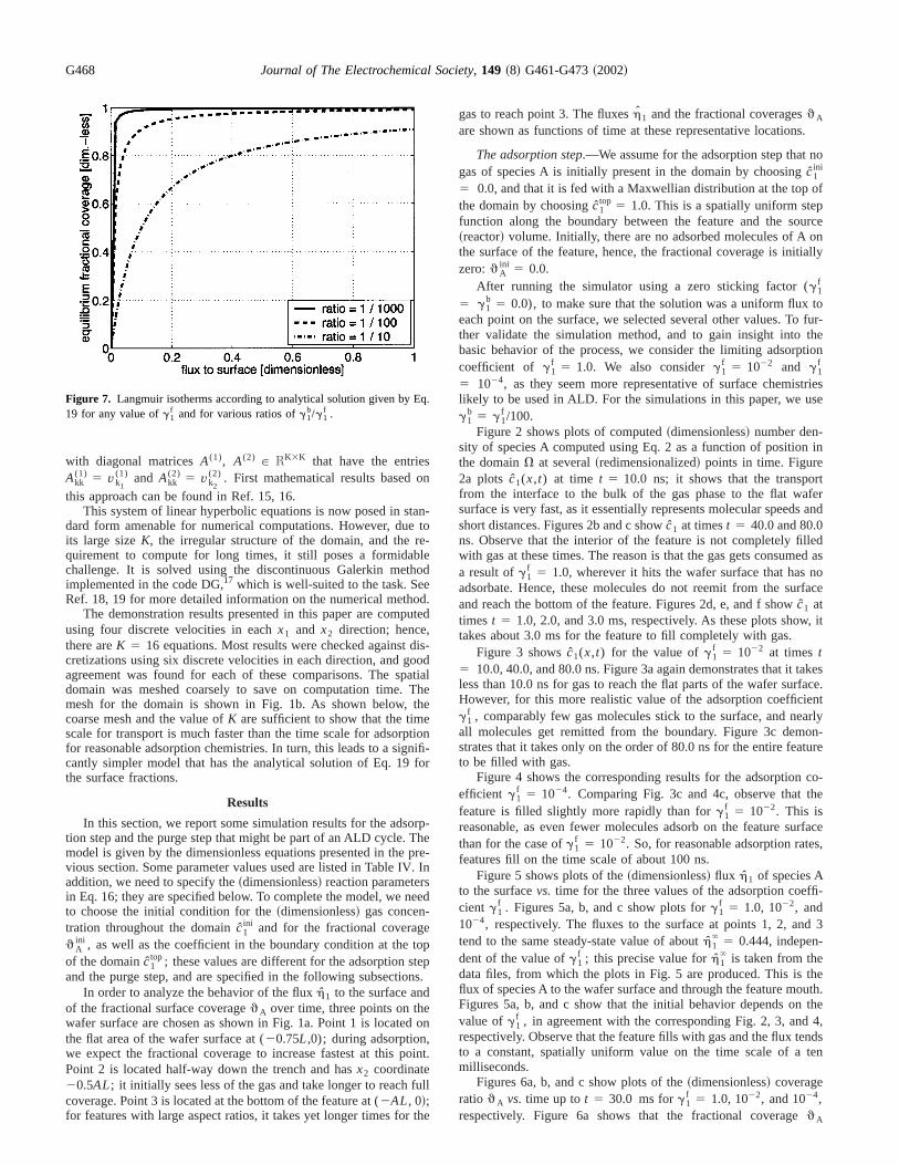
Figure 7. Langmuir isotherms according to analytical solution given by E19 for any value ofg1
f and for various ratios ofg1b/g1
f .
-o
d
.ed
-diale
n-
-ee-In
d
.
n
t.
l
e
gas to reach point 3. The fluxesh1 and the fractional coveragesqA
are shown as functions of time at these representative location
The adsorption step.—We assume for the adsorption step thatgas of species A is initially present in the domain by choosingc1
ini
5 0.0, and that it is fed with a Maxwellian distribution at the topthe domain by choosingc1
top 5 1.0. This is a spatially uniform stepfunction along the boundary between the feature and the so~reactor! volume. Initially, there are no adsorbed molecules of Athe surface of the feature, hence, the fractional coverage is initzero:qA
ini 5 0.0.After running the simulator using a zero sticking factor (g1
f
5 g1b 5 0.0), to make sure that the solution was a uniform flux
each point on the surface, we selected several other values. Tother validate the simulation method, and to gain insight intobasic behavior of the process, we consider the limiting adsorpcoefficient of g1
f 5 1.0. We also considerg1f 5 1022 and g1
f
5 1024, as they seem more representative of surface chemislikely to be used in ALD. For the simulations in this paper, we ug1
b 5 g1f /100.
Figure 2 shows plots of computed~dimensionless! number den-sity of species A computed using Eq. 2 as a function of positionthe domainV at several~redimensionalized! points in time. Figure2a plots c1(x,t) at time t 5 10.0 ns; it shows that the transpofrom the interface to the bulk of the gas phase to the flat wasurface is very fast, as it essentially represents molecular speedshort distances. Figures 2b and c showc1 at timest 5 40.0 and 80.0ns. Observe that the interior of the feature is not completely filwith gas at these times. The reason is that the gas gets consuma result ofg1
f 5 1.0, wherever it hits the wafer surface that hasadsorbate. Hence, these molecules do not reemit from the suand reach the bottom of the feature. Figures 2d, e, and f showc1 attimes t 5 1.0, 2.0, and 3.0 ms, respectively. As these plots showtakes about 3.0 ms for the feature to fill completely with gas.
Figure 3 showsc1(x,t) for the value ofg1f 5 1022 at timest
5 10.0, 40.0, and 80.0 ns. Figure 3a again demonstrates that it tless than 10.0 ns for gas to reach the flat parts of the wafer surHowever, for this more realistic value of the adsorption coefficieg1
f , comparably few gas molecules stick to the surface, and neall molecules get remitted from the boundary. Figure 3c demstrates that it takes only on the order of 80.0 ns for the entire feato be filled with gas.
Figure 4 shows the corresponding results for the adsorptionefficient g1
f 5 1024. Comparing Fig. 3c and 4c, observe that tfeature is filled slightly more rapidly than forg1
f 5 1022. This isreasonable, as even fewer molecules adsorb on the feature suthan for the case ofg1
f 5 1022. So, for reasonable adsorption ratefeatures fill on the time scale of about 100 ns.
Figure 5 shows plots of the~dimensionless! flux h1 of species Ato the surfacevs. time for the three values of the adsorption coefcient g1
f . Figures 5a, b, and c show plots forg1f 5 1.0, 1022, and
1024, respectively. The fluxes to the surface at points 1, 2, antend to the same steady-state value of abouth1
` 5 0.444, indepen-dent of the value ofg1
f ; this precise value forh1` is taken from the
data files, from which the plots in Fig. 5 are produced. This isflux of species A to the wafer surface and through the feature moFigures 5a, b, and c show that the initial behavior depends onvalue ofg1
f , in agreement with the corresponding Fig. 2, 3, andrespectively. Observe that the feature fills with gas and the flux teto a constant, spatially uniform value on the time scale of amilliseconds.
Figures 6a, b, and c show plots of the~dimensionless! coverageratio qA vs. time up tot 5 30.0 ms forg1
f 5 1.0, 1022, and 1024,respectively. Figure 6a shows that the fractional coverageqA
Journal of The Electrochemical Society, 149 ~8! G461-G473~2002! G469
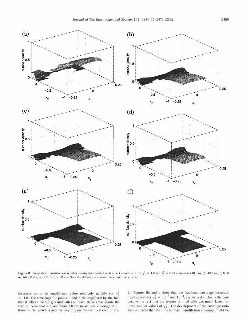
Figure 8. Purge step: dimensionless number density for a feature with aspect ratioA 5 4 for g1f 5 1.0 andg1
b 5 0.01 at times~a! 10.0 ns,~b! 40.0 ns,~c! 80.0ns, ~d! 1.0 ms,~e! 2.0 ms,~f! 3.0 ms. Note the different scales on thex1 and thex2 axes.
fact
t aig
seseforiot be
increases up to its equilibrium value relatively quickly forg1f
5 1.0. The time lags for points 2 and 3 are explained by thethat it takes time for gas molecules to reach those areas insidefeature. Note that it takes about 3.0 ms to achieve coverage athree points, which is another way to view the results shown in F
thell
.
2f. Figures 6b and c show that the fractional coverage increamore slowly forg1
f 5 1022 and 1024, respectively. This is the casdespite the fact that the feature is filled with gas much fasterthese smaller values ofg1
f . The development of the coverage ratalso indicates that the time to reach equilibrium coverage migh
d
ds
ical
asith
Journal of The Electrochemical Society, 149 ~8! G461-G473~2002!G470
inversely proportional to the value ofg1f , by comparing Fig. 6a and
b; Fig. 6c showsqA still in its initial linear phase and cannot be usefor this comparison.
The observations in Fig. 5 and 6 justify the approximation ofh1
in Eq. 18 by the constant, spatially uniform fluxh1` 5 0.444. Using
this value in Eq. 19 with initial conditionqAini 5 0.0, we are able to
obtain an analytical representation ofqA( t ). This analytical predic-tion is incorporated into the Fig. 6b and c as the solid diamonObserve the good agreement with the simulation results.
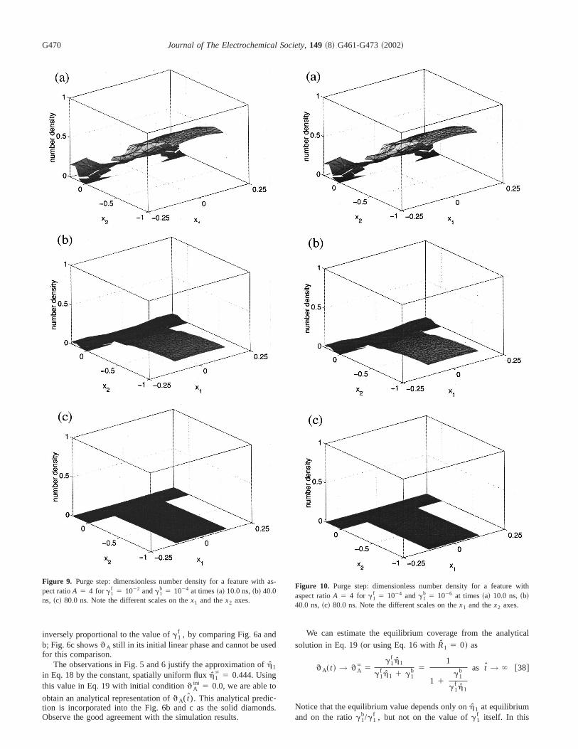
Figure 9. Purge step: dimensionless number density for a feature withpect ratioA 5 4 for g1
f 5 1022 andg1b 5 1024 at times~a! 10.0 ns,~b! 40.0
ns, ~c! 80.0 ns. Note the different scales on thex1 and thex2 axes.
.
We can estimate the equilibrium coverage from the analyt
solution in Eq. 19~or using Eq. 16 withR1 5 0! as
qA~ t ! → qA` 5
g1f h1
g1f h1 1 g1
b 51
1 1g1
b
g1f h1
as t → ` @38#
Notice that the equilibrium value depends only onh1 at equilibriumand on the ratiog1
b/g1f , but not on the value ofg1
f itself. In this
-Figure 10. Purge step: dimensionless number density for a feature waspect ratioA 5 4 for g1
f 5 1024 andg1b 5 1026 at times~a! 10.0 ns,~b!
40.0 ns,~c! 80.0 ns. Note the different scales on thex1 and thex2 axes.
eve
F
to
Journal of The Electrochemical Society, 149 ~8! G461-G473~2002! G471
study,h1 → 0.444 andg1b/g1
f 5 1/100, and we calculate the valuqA
` ' 0.977974, which is in excellent agreement with the observalues of 0.977975 and 0.977817 from the data used to generate6a and b, respectively.
Also based on the analytical result, we can predict the time
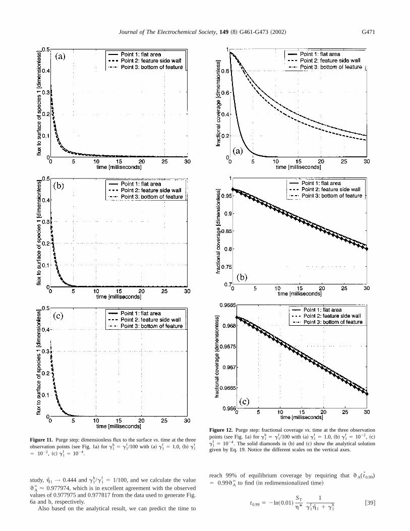
Figure 11. Purge step: dimensionless flux to the surfacevs. time at the threeobservation points~see Fig. 1a! for g1
b 5 g1f /100 with ~a! g1
f 5 1.0, ~b! g1f
5 1022, ~c! g1f 5 1024.
dig.
reach 99% of equilibrium coverage by requiring thatqA( t0.99)5 0.99qA
` to find ~in redimensionalized time!
t0.99 5 2ln~0.01!ST
h*1
g1f h1 1 g1
b @39#
Figure 12. Purge step: fractional coveragevs. time at the three observationpoints~see Fig. 1a! for g1
b 5 g1f /100 with ~a! g1
f 5 1.0, ~b! g1f 5 1022, ~c!
g1f 5 1024. The solid diamonds in~b! and ~c! show the analytical solution
given by Eq. 19. Notice the different scales on the vertical axes.
Journal of The Electrochemical Society, 149 ~8! G461-G473~2002!G472
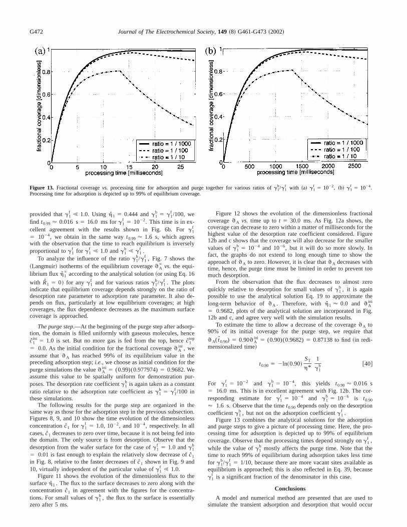
Figure 13. Fractional coveragevs. processing time for adsorption and purge together for various ratios ofg1b/g1
f with ~a! g1f 5 1022, ~b! g1
f 5 1024.Processing time for adsorption is depicted up to 99% of equilibrium coverage.
ely
o od
ghurf
p-ce
ee
urnt
thectioles
intth
f
thetha-ly
naler theurealler
the
too
ero
the
ig.
at
or-
n
ionpro-m
emee asuse
d toccur
provided thatg1f ! 1.0. Usingh1 5 0.444 andg1
b 5 g1f /100, we
find t0.99 ' 0.016 s5 16.0 ms forg1f 5 1022. This time is in ex-
cellent agreement with the results shown in Fig. 6b. Forg1f
5 1024, we obtain in the same wayt0.99 ' 1.6 s, which agreeswith the observation that the time to reach equilibrium is inversproportional tog1
f for g1f ! 1.0 andg1
b ! g1f .
To analyze the influence of the ratiog1b/g1
f , Fig. 7 shows the~Langmuir! isotherms of the equilibrium coverageqA
` vs. the equi-librium flux h1
` according to the analytical solution~or using Eq. 16
with R1 5 0! for any g1f and for various ratiosg1
b/g1f . The plots
indicate that equilibrium coverage depends strongly on the ratidesorption rate parameter to adsorption rate parameter. It alsopends on flux, particularly at low equilibrium coverages; at hicoverages, the flux dependence decreases as the maximum scoverage is approached.
The purge step.—At the beginning of the purge step after adsortion, the domain is filled uniformly with gaseous molecules, henc1
ini 5 1.0 is set. But no more gas is fed from the top, hencec1top
5 0.0. As the initial condition for the fractional coverageqAini , we
assume thatqA has reached 99% of its equilibrium value in thpreceding adsorption step;i.e., we choose as initial condition for thpurge simulations the valueqA
ini 5 (0.99)(0.977974)5 0.9682. Weassume this value to be spatially uniform for demonstration pposes. The desorption rate coefficientg1
b is again taken as a constaratio relative to the adsorption rate coefficient asg1
b 5 g1f /100 in
these simulations.The following results for the purge step are organized in
same way as those for the adsorption step in the previous subseFigures 8, 9, and 10 show the time evolution of the dimensionconcentrationc1 for g1
f 5 1.0, 1022, and 1024, respectively. In allcases,c1 decreases to zero over time, because it is not being fedthe domain. The only source is from desorption. Observe thatdesorption from the wafer surface for the case ofg1
f 5 1.0 andg1b
5 0.01 is fast enough to explain the relatively slow decrease oc1
in Fig. 8, relative to the faster decreases ofc1 shown in Fig. 9 and10, virtually independent of the particular value ofg1
f ! 1.0.Figure 11 shows the evolution of the dimensionless flux to
surfaceh1 . The flux to the surface decreases to zero along withconcentrationc1 in agreement with the figures for the concentrtions. For small values ofg1
b , the flux to the surface is essentialzero after 5 ms.
fe-
ace
-
n.s
oe
e
Figure 12 shows the evolution of the dimensionless fractiocoverageqA vs. time up to t 5 30.0 ms. As Fig. 12a shows, thcoverage can decrease to zero within a matter of milliseconds fohighest value of the desorption rate coefficient considered. Fig12b and c shows that the coverage will also decrease for the smvalues ofg1
b 5 1024 and 1026, but it will do so more slowly. Infact, the graphs do not extend to long enough time to showapproach ofqA to zero. However, it is clear thatqA decreases withtime, hence, the purge time must be limited in order to preventmuch desorption.
From the observation that the flux decreases to almost zquickly relative to desorption for small values ofg1
b , it is againpossible to use the analytical solution Eq. 19 to approximatelong-term behavior ofqA . Therefore, with h1 ' 0.0 and qA
ini
5 0.9682, plots of the analytical solution are incorporated in F12b and c, and agree very well with the simulation results.
To estimate the time to allow a decrease of the coverageqA to90% of its initial coverage for the purge step, we require th
qA( t0.90) 5 0.90qAini 5 (0.90)(0.9682)5 0.87138 to find~in redi-
mensionalized time!
t0.90 5 2ln~0.90!ST
h*1
g1b @40#
For g1f 5 1022 and g1
b 5 1024, this yields t0.90 ' 0.016 s5 16.0 ms. This is in excellent agreement with Fig. 12b. The cresponding estimate forg1
f 5 1024 and g1b 5 1026 is t0.90
' 1.6 s. Observe that the timet0.90 depends only on the desorptiocoefficientg1
b , but not on the adsorption coefficientg1f .
Figure 13 combines the analytical solutions for the adsorptand purge steps to give a picture of processing time. Here, thecessing time for adsorption is depicted up to 99% of equilibriucoverage. Observe that the processing times depend strongly ong1
f ,while the value ofg1
b mostly affects the purge time. Note that thtime to reach 99% of equilibrium during adsorption takes less tifor g1
b/g1f 5 1/10, because there are more vacant sites availabl
equilibrium is approached; this is also reflected in Eq. 39, becag1
f is a significant fraction of the denominator in this case.
Conclusions
A model and numerical method are presented that are usesimulate the transient adsorption and desorption that would o
uiseedpa
omr
eosu
an, t
e
mur aceeco-
daroman
Real
l
teirchcle
os
try
ries,
la-
-
ture
. K.
Journal of The Electrochemical Society, 149 ~8! G461-G473~2002! G473
during ALD over micrometer scale features during integrated circfabrication. The assumptions for the Boltzmann equation-bamodel are presented, and no adjustable parameters are ussimple reversible Langmuir adsorption model is used; kineticrameter values are chosen for demonstration purposes.
We consider the case in which the flux of reactive species frthe source volume to the wafer surface is constant in time, eithezero or at some selected values;i.e., we idealize transients at threactor scale, to focus on modeling feature scale transients. Mgeneral boundary conditions at the interface between the waferface and the reactor volume are certainly possible.
We present results for transients in number density, flux,surface coverage, and show that for reasonable surface kineticstime scale for transport~'100 ns! is much shorter than the timscale for adsorption and desorption~milliseconds to seconds!. Thishas significant implications for integrated multiscale process silation, as it allows the resolution in time to be of the same ordeprocess transients. Thus, previous integrated multiscale prosimulation efforts can be extended to model pattern scale effduring transients.20-22 These transients can be intrinsic or prgrammed to optimize some process or product property.8
Acknowledgments
M.K.G. acknowledges support by the National Science Fountion under grant DMS-9805547. T.S.C. acknowledges support fMARCO, the Defense Advanced Research Projects Agency,New York State Office of Science, Technology, and Academicsearch through the Interconnect Focus Center. The authorsthank the International Erwin Schro¨dinger Institute for TheoreticaPhysics~Vienna, Austria! for the kind hospitality and support whilewriting this paper. We also acknowledge support of the WittgensAward 2000 of P. Markowich, financed by the Austrian ReseaFund. Finally, we are grateful to C. Ringhofer and J.-F. Remawithout whose help this work would not have been possible.
Rensselaer Polytechnic Institute assisted in meeting the publication cof this article.
td. A-
at
rer-
dhe
-sssts
-
d-so
n
,
ts
References
1. M. Ritala and M. Leskela,Nanotechnology,10, 19 ~1999!.2. M. Leskela and M. Ritala,J. Phys. IV,5, 937 ~1995!.3. T. Suntola,Thin Solid Films,216, 84 ~1992!.4. H. Simon and J. Aarik,J. Phys. D,30, 1725~1997!.5. T. S. Cale, T. P. Merchant, L. J. Borucki, and A. H. Labun,Thin Solid Films,365,
152 ~2000!.6. T. S. Cale and V. Mahadev, inThin Films, Vol. 22, p. 175, Academic Press, New
York ~1996!.7. T. S. Cale, T. P. Merchant, and L. J. Borucki, inProceedings of the Advanced
Metallization Conference in 1998, Materials Research Society, p. 737~1999!.8. T. S. Cale, D. F. Richards, and D. Yang,J. Comput.-Aided Mater. Des.,6, 283
~1999!.9. M. K. Gobbert and T. S. Cale, inFundamental Gas-Phase and Surface Chemis
of Vapor-Phase Deposition II, M. T. Swihart, M. D. Allendorf, and M. Meyyappan,Editors, PV 2001-13, p. 316. The Electrochemical Society Proceedings SePennington, NJ~2001!.
10. C. Cercignani,The Boltzmann Equation and Its Applications, Springer-Verlag, NewYork ~1988!.
11. C. Cercignani,Rarefied Gas Dynamics: From Basic Concepts to Actual Calcutions, Cambridge University Press, New York~2000!.
12. G. N. Patterson,Introduction to the Kinetic Theory of Gas Flows, University ofToronto Press, Ontario, CN~1971!.
13. R. I. Masel,Principles of Adsorption and Reaction on Solid Surfaces, Wiley Inter-science, New York~1996!.
14. C. Ringhofer,Acta Numer.,6, 485 ~1997!.15. M. K. Gobbert and C. Ringhofer, inIMA Volumes in Mathematics and Its Appli
cations, Springer-Verlag, New York, Accepted for publication.16. M. K. Gobbert and C. Ringhofer,Multiscale Modeling and Simulation, Submitted.17. J.-F. Remacle, J. Flaherty, and M. Shephard,SIAM J. Sci. Comput. (USA),Ac-
cepted for publication.18. Discontinuous Galerkin Methods: Theory, Computation and Applications; Lec
Notes in Computational Science and Engineering, B. Cockburn, G. E. Karniadakis,and C.-W. Shu, Editors, Vol. 11, Springer-Verlag, New York~2000!.
19. M. K. Gobbert, J.-F. Remacle, and T. S. Cale, Unpublished work.20. M. K. Gobbert, T. P. Merchant, L. J. Borucki, and T. S. Cale,J. Electrochem. Soc.,
144, 3945~1997!.21. T. P. Merchant, M. K. Gobbert, T. S. Cale, and L. J. Borucki,Thin Solid Films,365,
368 ~2000!.22. T. S. Cale, M. O. Bloomfield, D. F. Richards, K. E. Jansen, J. A. Tichy, and M
Gobbert, inIMA Volumes in Mathematics and Its Applications, Springer-Verlag,New York, Accepted for publication.