Transforming Constraint Diagrams

Jim Burton∗ Gem Stapleton†

Ali Hamie‡

Visual Modelling GroupUniversity of Brighton, Brighton, UK

August 17, 2009

Abstract

Constraint diagrams were proposed by Kent for the purposes of formal soft-ware specification in a visual manner. They have recently been formalized andgeneralized, making them more expressive. This paper presents a collection oftransformations that can be applied to the so-called unitary α fragment of con-straint diagrams. The transformations can be used to define inference rules in amore succinct manner than in earlier systems. We establish that the transforma-tions are sufficient to transform any given unitary α-diagram into any other unitaryα-diagram. Therefore, they are sufficient for formalizing any inference rules be-tween such diagrams.

1 IntroductionVisual languages play an important role in the design and implementation of software.For example, the Unified Modelling Language (UML) [20] is now an industry standardvisual notation designed specifically for use by software engineers and is used through-out the software development process, from capturing domain requirements through toimplementation. Under some circumstances (such as in a safety critical environment;see, for example, [19]) it is desirable, perhaps even essential, to produce formal modelsof software. In part, such application areas serve to motivate the need for the precisespecification of the UML at both a syntactic and semantic level; the pUML group wasset up with this goal in mind [18].

Part of the creation of a formal model is likely to involve specifying constraints suchas system invariants and operation contracts which, within the UML, is achieved byusing the Object Constraint Language (OCL) [22]. The OCL is the only purely textualpart of the UML and, therefore, does not fit with the UML’s diagrammatic theme.Building on the formal diagrammatic reasoning systems of Shin [13], Hammer [1] and∗ j.burton@brighton.ac.uk† g.e.stapleton@brighton.ac.uk‡ a.a.hamie@brighton.ac.uk

62

others, Kent introduced constraint diagrams [11] which are designed to complementthe visual components of the UML and to specify constraints like the (symbolic) OCL.Constraint diagrams can also be used independently of the UML.

In figure 1 there is a constraint diagram which expresses an invariant that we mightwish to place on a video rental store system: there is a member that can only borrowfilms that are in the collections of the stores which they have joined. The semantics ofconstraint diagrams will be explained more fully later, but the blob acts as an existentialquantifier, the arrows allow us to make statements about binary relations and the closedcurves represent sets (or classes).

canBorrow

collectionjoined

Member. Film

Store

Figure 1: A constraint diagram.

At first glance, constraint diagrams appear intuitive and, perhaps, unambiguous, butit was not until a formalization of their semantics was attempted that a range of ambi-guities was noticed [8]. Indeed, only when a formalization was eventually obtained [5]did the complexity of interpreting these diagrams become apparent. Whilst in manyexamples constraint diagrams are “well-matched to meaning” [9] there are also manysituations where their intuitiveness breaks down. This led to the development of gen-eralized constraint diagrams [14]. Both of these constraint diagram notations share acommon fragment, which is considered in this paper. For this fragment, we set up atransformation system which forms the basis of a reasoning system for both constraintdiagrams and generalized constraint diagrams.

There are various ways in which reasoning will need to be performed when usingformal methods. First, there is reasoning about the model; for example, when onewishes to show that the model is consistent or that the post-condition of one operationimplies the precondition of another. Secondly, a programmer will need to use someinformal reasoning to determine an appropriate implementation that conforms to thespecification. Thirdly, at a later stage, one might also wish to formally prove thatthe implementation does indeed conform to the model. Formal reasoning has beeninvestigated for constraint diagrams [4, 16] but as yet no inference rules have beendefined for generalized constraint diagrams.

An aim of this paper is to define a transformation system for so-called unitary α-diagrams which can be used to subsequently define inference rules for either constraintdiagrams or generalized constraint diagrams. Section 2 provides a brief overview ofunitary diagrams. We also present a formalization of the syntax of unitary diagrams in

63

section 2. Our transformations are defined in section 3, focusing separately on thosewhich remove syntax and those which add syntax. Finally, in section 4, we show howthe transformations can be used as a basis for inference rules.

2 Unitary DiagramsWe follow a typical approach of formally defining the syntax at an abstract level [10].In this way, we disregard the many aspects of drawn diagrams that are irrelevant to theirsemantic meaning, such as the shape and relative location of curves. To aid intuition,we include a informal presentation of the concrete syntax, since this is used to guidethe work, but all formal aspects are conducted at the abstract level.

2.1 Concrete SyntaxThe concrete syntax of a visual language defines, in our case, diagrams as drawn im-ages. We proceed to sketch the concrete syntax of so-called unitary constraint dia-grams. We make occasional reference to semantics to aid the readers’ understanding.For the purposes of this paper, the semantics are not particularly important, which iswhy we do not include their precise formalization.

Unitary constraint diagrams consist of closed curves (some of which may be la-belled) drawn in the plane and which represent sets. The spatial relationships betweenthe curves makes assertions about the relationships between the represented sets. Forexample, the diagram in figure 1 contains six curves, three of which are labelled. Theplacement of one curve inside another makes a subset assertion, whilst non-overlappingcurves make a disjointness assertion. So, Member and Film are disjoint, for example.

In the regions formed by the curves we can place graphs, whose nodes are either alldots or all asterisks; these graphs are called existential spiders and universal spiders re-spectively. Existential spiders represent the existence of an element. In figure 1, there isone existential spider that has exactly one node placed inside Member . For simplicityof presentation, we will assume there are no universal spiders, although the transforma-tions we define can easily be extended to cope with their inclusion. Similarly, we alsoassume that the existential spiders are placed in single zones; this constraint to singlezones gives what are called α-diagrams [16]. The curves in a diagram subdivide theplane into minimal regions: such a region is a connected component of the plane lessthe images of the curves. In figure 1, there are seven minimal regions. Of particularimportance is the notion of a zone in a diagram, d. A zone is a set of minimal regionsthat can be described as being inside some (possibly no) curves but outside the restof the curves in d. Semantically, a zone represents the set which is the intersection ofthe sets represented by the curves it is inside less the union of the sets represented bythe curves that it is outside. In figure 1, every minimal region is also a zone and thereare no zones that are not also minimal regions. However, this need not be the case:sometimes, zones consist of more than one minimal region and such zones are said tobe disconnected. Zones can be shaded. The use of shading places an upper bound onthe cardinality of the represented sets: in a shaded zone, all of the elements must berepresented by spiders.

64

Finally, arrows are used to make statements about binary relations: the set of ele-ments (or element) represented by the arrow’s source is related to precisely the set ofelements represented by the arrow’s target under the relation represented by the arrow’slabel. For example, in figure 1 the arrow labelled joined sourced on the existential spi-der, e, asserts that the set of elements to which e is related under the relation joined isa subset of Store. In addition, if we restrict the domain of collection to Store then weobtain a subset of Film which includes all of the films that can be borrowed by e.

So far, we have described unitary diagrams which consist of curves, spiders placedin zones or sets of zones, shading, and arrows. Further examples of unitary diagramscan be seen throughout the paper; we discuss the syntax of d1 when presenting theformalization below. We refer the reader to [5] for further examples and more precisedetails on the concrete syntax and the semantics of constraint diagrams, and to [14]for similar information on generalized constraint diagrams. For the purposes of thispaper, it is the formal, abstract, syntax that is important and the next section includesthose details necessary for our transformations to be defined. Unitary diagrams can bejoined together using logical connectives, such as ∧, to make compound diagrams; it isunitary diagrams for which we define transformations.

We have placed a restriction on spiders so that they can only have one node, mean-ing that they are placed inside single zones. This restriction yields α-diagrams whichform a fragment of (non-unitary) generalized constraint diagrams that is not reduced inexpressive power: given any generalized constraint diagram there exists a semanticallyequivalent diagram that contains only spiders placed inside single zones. However,there are constraint diagrams that are not semantically equivalent to any α-diagram,but only if they contain universal spiders. That is given a constraint diagram contain-ing only existential spiders, one can reduce it to an α-diagram,as in [16]. We note thatexcluding universal spiders does decrease the expressive power but, as stated above,our work easily adapts to the case where they are permitted.

2.2 Abstract SyntaxOur formal definition of the syntax of unitary diagrams adapts that in [14]. In theabstract syntax we identify labelled curves with their labels; curve labels are drawnfrom the set LC. Further, at the abstract level, the unlabelled curves are formalizedas elements of an arbitrary (but specified) set UC. We consider the elements of UC tocorrespond directly to the unlabelled curves of drawn diagrams. In a drawn diagram, azone can be described by the curves that contain it and the curves that do not containit. We use this insight to formalize zones at an abstract level.

Definition 2.1. A zone is a pair, (in, out) where in ∩ out = ∅ and in∪out ⊆ LC∪UC.

The set of all zones is denoted Z . To illustrate the concept, the shaded zone infigure 2 can be described by z = ({A}, {B, uc}) where uc denotes the unlabelledcurve. There are two spiders placed in this zone; we cannot formalize a spider byidentifying it with the zone in which it is placed. However, this provides the basis oftheir formalization: a spider will essentially be defined as a number together with azone. In our example, the two spiders are written as s1(z) and s2(z).

65

.A

d1 d2

.B

l

.A

.l

Figure 2: Formalizing the syntax.

Definition 2.2. A spider is of the form si(z) where i is a natural number and z is azone. The habitat of si(z) is z and we say that si(z) inhabits z.

The set of all spiders is denoted S. We now proceed to formalize arrows. Toidentify the arrows in a drawn diagram, it is sufficient to state their source and target,together with their label. For example, in figure 2, the arrow can be described by thetriple (l, s1(z), uc) (recall, uc is the unlabelled curve and z = ({A}, {B, uc})). Wedraw arrow labels from a fixed set AL.

Definition 2.3. An arrow end is either a curve drawn from LC ∪UC or a spider drawnfrom S. An arrow is an ordered triple (l, s, t) where l ∈ AL, and s and t are arrowends called the source and target respectively.

Definition 2.4. A unitary diagram is a tuple, d = (Z,Z∗, S,A), which satisfies thefollowing:

1. Z = Z(d) is a finite set of zones such that for each pair of zones (in1, out1) and(in2, out2) in Z(d) we have in1 ∪ out1 = in2 ∪ out2. That is, the zones are alldescribed using the same curves. We define C(d) = in1 ∪ out1.

2. Z∗ = Z∗(d) is a set of shaded zones such that Z∗(d) ⊆ Z(d). That is, all of theshaded zones are in the diagram.

3. S = S(d) is a finite set of spiders such that for each spider si(z) ∈ S(d),z ∈ Z(d). That is, spiders are placed in zones of the diagram.

4. A = A(d) is a set of arrows such that for each arrow (l, s, t) in A(d), s and tare in S(d) ∪ C(d). That is, arrows are sourced and targeted on components ofthe diagram.

So, d1 in figure 2 is formalized as the tuple (Z,Z∗, S,A) where:

1. Z is comprised of the following zones.

• ({A}, {B, uc}),• ({A,B}, {uc}),• ({B}, {A, uc}),

66

• ({B, uc}, {A}),• ({uc}, {A,B}),• (∅, {A,B, uc})

2. Z∗ = {({A}, {B, uc})},

3. S = {s1({A}, {B, uc}), s2({A}, {B, uc})}, and

4. A = {(l, s1({A}, {B, uc}), uc)}.

Semantically, d1 asserts that the set A − B contains at least two elements, x and y,through the use of the two existential spiders, the shading asserts that there are no moreelements in that set (i.e. |A − B| = 2), and that x is related to some set of elements,say x.l, under the relation l such that x.l ∩ A = ∅. The diagram d2 makes a weakerstatement, asserting that there are at least two elements in A, at least one of which isrelated to some set of elements, under l, that is disjoint from A. In fact, we can deduced2 from d1 and, if we had a set of sound and (possibly) complete inference rules thenwe could prove that d2 does indeed follow semantically from d1.

3 TransformationsTo facilitate elegant definitions of inference rules for unitary diagrams, we define di-agram transformations, which are purely syntactic and represent the addition or re-moval of a piece of syntax. For example, we can remove the curve B from d1 infigure 2, transforming it into d2; this remove curve transformation will be formalizedbelow. The transformations defined will be applicable under specified syntactic con-ditions, which are not related to sound reasoning, but are intended to merely constrainthe transformation to ensure the result of its application is a diagram. The benefit ofmaking transformations which are purely syntactic and unrelated to reasoning is thatthis facilitates their use in a wide number of (reasoning) contexts.

3.1 Transformations that remove syntaxWe start with the simplest transformation, that which removes an arrow.

Transformation 1. Remove arrow

We can transform a diagram by removing an arrow. In figure 3, the arrow, a, labelled ris removed from d1 to give d2.Formal definition Let d1 be a unitary diagram such that there exists an arrow a inA(d1). The diagram d2 can be obtained from d1 removing a using the remove arrowtransformation, denoted d1

−a−→ d2, where d2 = (Z(d1), Z∗(d1), S(d1), A(d1)−{a}).

67

.A

d1 d2

-a

r .A

Figure 3: Transforming a diagram by removing an arrow.

Transformation 2. Remove shading

We can transform a diagram by removing the shading from a zone. In figure 4, theshading is removed from the zone ({B}, {A}) in d1 to give d2.

A

d1 d2

-z*

AB B

Figure 4: Transforming a diagram by removing shading from a zone.

Formal definition Let d1 be a unitary diagram and let z be a zone such that z ∈Z∗(d1). The diagram d2 can be obtained from d1 using the remove shading transfor-

mation, denoted d1−z∗−→ d2, where d2 = (Z(d1), Z∗(d1)− {z}, S(d1), A(d1)).

Transformation 3. Remove spider

Our next transformation removes a spider from a unitary diagram. We need to providea constraint (i.e. a precondition) on when this transformation can be applied in order toensure that the result is a diagram. To formally define the remove spider transformation,we need to refer to the set of arrows sourced on, or targeting, a spider. Later, we alsoneed to identify curves that are the source or target of an arrow. Here, we provide somenotation that is convenient for identifying these sets.

Definition 3.1. Let d be a unitary diagram and let s be a spider in S(d). The set ofarrows which are either sourced or targeted on s in d, denoted A(s, d), is

A(s, d) = {(l, σ, τ) ∈ A(d) : σ = s ∨ τ = s}.

If an arrow a is sourced or targeted on s then we say a touches s. Similarly, we definethe set of arrows which touch a curve c in a diagram d, denoted A(c, d):

A(c, d) = {(l, σ, τ) ∈ A(d) : σ = c ∨ τ = c}.

68

We can transform diagrams by removing a spider provided it is not touched by anarrow. In figure 5 s is removed from d1 to give d2.

d1 d2

-s. .r

.r

s

Figure 5: Transforming a diagram by removing a spider.

Formal definition Let d1 be a unitary diagram such that there exists a spider s ∈ S(d1)which is not touched by any arrow, that isA(s, d) = ∅. The diagram d2 can be obtainedfrom d1 by removing s under the remove spider transformation, denoted d1

−s−→ d2,where d2 = (Z(d1), Z∗(d1), S(d1)− {s}, A(d1)).

Transformation 4. Remove zone

We can transform a diagram by removing any zone which is not the habitat of anyspider. In figure 6 the zone ({A,B}, ∅) is removed from d1 to give d2.

d1 d2

-z

A B A B

Figure 6: Transforming a diagram by removing a zone.

Formal definition Let d1 be a unitary diagram such that there exists a zone z in Z(d1)which is not the habitat of any spider. Then the diagram d2 can be obtained fromd1 by removing z under the remove zone transformation, denoted d1

−z−→ d2, whered2 = (Z(d1)− {z}, Z∗(d1)− {z}, S(d1), A(d1)).

Transformation 5. Remove curve

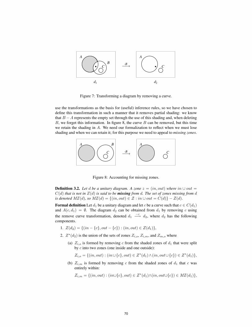
We can remove a curve provided it is not touched by any arrow. In figure 7 the curvelabelled B is removed from d1 to give d2.

In diagram d1 in figure 7, the region inside the curve labelled A is partially shaded.We could choose to define the transformation which removes B so that it removesthis partial shading or leaves as shaded all zones which were shaded in the original.Actually, there are various choices for how to define a remove curve rule. We want to

69

d1 d2

-B

A

BC.

A

C.

Figure 7: Transforming a diagram by removing a curve.

use the transformations as the basis for (useful) inference rules, so we have chosen todefine this transformation in such a manner that it removes partial shading: we knowthat B−A represents the empty set through the use of this shading and, when deletingB, we forget this information. In figure 8, the curve B can be removed, but this timewe retain the shading in A. We need our formalization to reflect when we must loseshading and when we can retain it; for this purpose we need to appeal to missing zones.

-B

A

C

B A

C

Figure 8: Accounting for missing zones.

Definition 3.2. Let d be a unitary diagram. A zone z = (in, out) where in ∪ out =C(d) that is not in Z(d) is said to be missing from d. The set of zones missing from dis denoted MZ (d), so MZ (d) = {(in, out) ∈ Z : in ∪ out = C(d)} − Z(d).

Formal definition Let d1 be a unitary diagram and let c be a curve such that c ∈ C(d1)and A(c, d1) = ∅. The diagram d2 can be obtained from d1 by removing c usingthe remove curve transformation, denoted d1

−c−→ d2, where d2 has the followingcomponents.

1. Z(d2) = {(in− {c}, out− {c}) : (in, out) ∈ Z(d1)},

2. Z∗(d2) is the union of the sets of zones Zi,o, Zi,m, and Zm,o where

(a) Zi,o is formed by removing c from the shaded zones of d1 that were splitby c into two zones (one inside and one outside):

Zi,o = {(in, out) : (in∪{c}, out) ∈ Z∗(d1)∧ (in, out∪{c}) ∈ Z∗(d1)},

(b) Zi,m is formed by removing c from the shaded zones of d1 that c wasentirely within:

Zi,m = {(in, out) : (in∪{c}, out) ∈ Z∗(d1)∧(in, out∪{c}) ∈ MZ (d1)},

70

(c) Zm,o is formed by removing c from the shaded zones of d1 that c wasentirely outside:

Zm,o = {(in, out) : (in∪{c}, out) ∈ MZ (d1)∧(in, out∪{c}) ∈ Z∗(d1)},

3. S(d2) = {si(in− {c}, out− {c}) : si(in, out) ∈ S(d1)},

4. A(d2) = A(d1).

3.2 Transformations that add syntaxThe transformations that we define for adding syntax are counterparts of those whichremove syntax. For the first two transformations no examples are given since they arevery similar to their remove syntax counterparts.

Transformation 6. Add arrow

Formal definition Let d1 be a unitary diagram and let (l, s, t) be an arrow such thats, t ∈ S(d) ∪ C(d) and (l, s, t) 6∈ A(d1). The diagram d2 can be obtained by adding(l, s, t) to d1 using the add arrow transformation, denoted d1

+a−→ d2, where d2 =(Z(d1), Z∗(d1), S(d1), A(d1) ∪ {(l, s, t)}).

Transformation 7. Add spider

Formal definition Let d1 be a unitary diagram such that there exists a zone z ∈ Z(d1)and a spider si(z) 6∈ S(d1) where z ∈ Z(d1). The diagram d2 can be obtained byadding s to d1 using the add spider transformation, denoted d1

+s−→ d2, where d2 =(Z(d1), Z∗(d1), S(d1) ∪ {s}, A(d1)).

Transformation 8. Add shading

We can transform a diagram by adding shading to a zone. In figure 9, shading is addedto the zone ({A,C}, {B}) in d1 to give d2.

d1 d2

+z*

A B

C

A B

C

Figure 9: Transforming a diagram by adding shading to a zone.

Formal definition Let d1 be a unitary diagram and z ∈ Z(d1)−Z∗(d1). The diagramd2 can be obtained from d1 by adding shading to z using the add shading transforma-

tion, denoted d1+z∗−→ d2, where d2 = (Z(d1), Z∗(d1) ∪ {z}, S(d1), A(d1)).

71

d1 d2

+z

A Bf

A Bf

CC

Figure 10: Transforming a diagram by adding a zone.

Transformation 9. Add zone

We can transform a diagram by adding a missing zone. Figure 10 shows the additionof the missing zone ({A,B}, {C}) to d1 to give d2.Formal definition Let d1 be a unitary diagram and z be a zone such that z ∈ MZ (d1).The diagram d2 can be obtained from d1 by adding z using the add zone transformation,denoted d1

+z−→ d2, where d2 = (Z(d1) ∪ {z}, Z∗(d1), S(d1), A(d1)).

Transformation 10. Add curve

There are a number of ways of adding a curve to a diagram: the new curve can be addedin such a way that it is entirely outside of all existing curves, or is entirely containedwithin one other curve, and so on. The relationship between the new curve and theexisting curve can be captured by appealing to its relationship with the existing zones:the existing zones are either completely inside the new curve, completely outside thenew curve, or split by the new curve. Thus, we parametrise the transformation ofadding a curve to a diagram d1 using two subsets of zones which we call Zin and Zout,where Zin∪Zout = Z(d1); those zones which will fall inside the new curve are in Zin,those outside in Zout and those that will be split are in Zin ∩Zout. The case of addinga curve which splits every zone in d1, for instance, is that of choosing Zin = Zout =Z(d1). Figure 11 shows an example of adding a curve with Zin = {(∅, {A,B})} andZout = Z(d1)− Zin.

In addition, each spider can be inside or outside the new curve. Thus, we alsosupply a two-way partition of the spider set, Sin and Sout, allowing us to specify thehabitats of the spiders after the curve addition. We must place constraints on the choiceof Sin and Sout to ensure consistency with the manner in which the curve is added.For instance, we cannot place a spider si(z) in the set Sin if z ∈ Zout −Zin, since the‘new’ habitat of the spider will not be present in the diagram after the curve addition.Consequently, we only have a choice about whether a spider, si(z), is in Sin or Sout ifz ∈ Zin ∩ Zout. Note that this is a syntactic constraint and not related to soundness.An appropriate choice of Zin, Zout, Sin and Sout allows the user to add curves in anyof the possible ways.

Recall that the set LC ∪ UC is the abstract set that corresponds to the labelled andunlabelled curves that can appear in any diagram at the concrete syntax level. The setC(d), for any unitary diagram d, is a subset of LC ∪ UC.

72

d

+c

A

r B

C

. .A

r B

. .

1 d2

Figure 11: Transforming a diagram by adding a curve.

Formal definition Let d1 be a unitary diagram and let c be a curve that is not in d1,that is c ∈ (LC ∪ UC) − C(d). Let Zin and Zout be subsets of Z(d1) such thatZin ∪ Zout = Z(d1). Let Sin and Sout be a two-way partition of S(d1) such that

1. for all si(z) in Sin, z ∈ Zin and

2. for all si(z) in Sout, z ∈ Zout.

The diagram d2 can be obtained by adding the curve c to d1 using the add curve trans-formation, denoted d1

+P−→ d2, where P = (c, Zin, Zout, Sin, Sout) and d2 has thefollowing components:

1. Z(d2) = Zin+c ∪ Zout+c where

(a) Zin+c is formed by adding c to the zones of d1 that we wish to contain c ind2: Zin+c = {(in ∪ {c}, out) : (in, out) ∈ Zin},

(b) Zout+c is formed by adding c to the zones of d1 that we wish to exclude cin d2: Zout+c = {(in, out ∪ {c}) : (in, out) ∈ Zout}.

2. Z∗(d2) = Z∗in+c ∪ Z∗out+c where

(a) Z∗in+c = {(in ∪ {c}, out) : (in, out) ∈ Zin ∩ Z∗(d1)},(b) Z∗out+c = {(in, out ∪ {c}) : (in, out) ∈ Zout ∩ Z∗(d1)}.

3. S(d2) = Sin+c ∪ Sout+c where

(a) Sin+c = {si(in ∪ {c}, out) : si(in, out) ∈ Sin},(b) Sout+c = {si(in, out ∪ {c}) : si(in, out) ∈ Sout}.

4. A(d2) = A(d1).

3.3 Completeness of the TransformationsThe set of transformations defined above is complete because we can use them to trans-form any unitary diagram into any other unitary diagram, although the resulting systemis (intentionally) not sound. The completeness of the transformation system means thatthese transformations are sufficient for describing a set of sound and complete inferencerules for the unitary α-diagram fragment of both constraint diagrams and generalizedconstraint diagrams.

73

Theorem 1. Let d1 and dn be unitary diagrams. Then there exists a sequence ofdiagrams, (d1, d2..., dn) such that for each i, where 1 < i ≤ n, the diagram di canbe obtained from di−1 by the application of one of the above transformations. In otherwords, the given set of transformations is complete.

Sketch. The transformations which remove syntax can be used repeatedly to transformd1, regardless of its content, into the diagram (∅, ∅, ∅, ∅). The transformations whichadd syntax can then be used to build d2.

Although there will often be faster ways to transform one diagram into another, wecan rely on the ‘brute force’ method of removing all diagrammatic elements from d1 toproduce the empty diagram then adding the elements of d2. This relies on choosing theright order in which to apply the transformations, depending on their pre-conditions ofsyntactic well-formedness; for instance, before using remove spider (transformation 3)to remove a spider s which is the source of an arrow a in d1, we must first use removearrow (transformation 1) to remove a from d1.

4 Using Transformations to Define Inference Rules

We are able to use the transformations to define inference rules in a variety of ways.The motivation for using transformations in this way is by analogy with software en-gineering. Functional and modular abstraction leads to systems with less code dupli-cation and which are easier to understand and maintain. In a similar way, the shorterinference rule definitions that result from abstracting syntactic details into transforma-tions are easier to state, reason about and check for errors. We are able to composetransformations in the definition of rules which make several changes to a diagram in asimilar way to composing referentially transparent functions in a functional program-ming language. To use the transformations when defining inference rules, we may needto place further conditions on when the transformation can be applied to ensure sound-ness. In the case of the erasure of a spider, such a condition would be that the habitatis not shaded.

We have defined a set of sound inference rules for the unitary α fragment of gen-eralized constraint diagrams, and present three of their definitions below as examples.Work on establishing a complete set for this fragment is ongoing. Four transformationscan immediately be used as sound inference rules: remove arrow, remove shading,remove curve and add zone. The other transformations need not result in a semanticconsequence of the diagram to which they are applied. Some transformations are usedby several rules; for instance, (at least) five of inference rules that we have so far de-fined use the add arrow transformation. An add shaded zone inference rule makes useof two transformations. We have also begun work on defining inference rules whoseapplication results in a compound diagram, and expect a significant proportion of theseinference rules to use more than one of the transformations defined here, particularlyas compared to the unitary fragment, because the compound inference rules tend to bemore complex.

74

A

.B

C.l

d1

A

.C.l

d2

A

.C.l

d3

l A

.C.l

d4

l

Figure 12: Using transformations to define inference rules.

To illustrate how we use the transformations to define sound inference rules, weconsider an example. Figure 12 shows a proof of d4 from d1. First, we apply theremove curve transformation to d1 giving d2. We note that the remove curve transfor-mation can be used directly as an inference rule; that is, applying the remove curvetransformation always results in a semantic consequence of the diagram to which thetransformation is applied. Next, we apply an add arrow rule to give d3. Unlike theremove curve transformation, we cannot add arrows in arbitrary ways and obtain a se-mantic consequence. The information provided by the new arrow must be deduciblefrom the information already present in the diagram and, as stated, we have defined anumber of rules which add arrows. The rule used to obtain d3 from d2 is called Addarrow: contour to spider. Before defining the rule, we define the empty curves of adiagram, or those within which every zone is shaded.

Definition 4.1. Let d be a unitary diagram. Define the empty curves of d, denotedEC (d), as follows.

EC (d) = {c ∈ C(d) : ∀(in, out) ∈ Z(d) c ∈ in⇒ (in, out) ∈ Z∗(d)}.

Definition 4.2. Add arrow: contour to spider. Let d1 be a unitary diagram such that:

1. there is an arrow (l, s, t) in A(d1) such that t ∈ EC (d1), and

2. there is a spider σ ∈ S(d1) such that S(t, d1) = {σ}.

Let d2 be the diagram obtained by adding the arrow (l, s, σ) to d1 using the add arrowtransformation. Then we may replace d1 with d2.

As an example of the reuse of transformations, we include a second inference rulewhich adds an arrow to a diagram. Informally, diagram d1 in figure 13 tells us that

75

the sum of the images of the relation r when restricted to the elements of A is theempty set. This information is provided by the arrow labelled r which is sourced on Aand targets the shaded and unlabelled curve. It follows that we can add an arrow withthe same source and label which targets any other empty curve without changing themeaning of the diagram. The inference rule Add arrow: empty set allows us to do thisand is used in d2 to add an arrow with the same source and label as the arrow in d1 butwhich targets B.

A

B

rA

B

r

r

d1 d2

Figure 13: An application of the inference rule Add arrow: empty set.

Definition 4.3. Add arrow: empty set. Let d1 be a unitary diagram which satisfies:

1. there is an arrow (l, s, t) in A(d1) where t ∈ EC (d1),

2. there is a curve t1 ∈ EC (d1) where (l, s, t1) 6∈ A(d1).

Let d2 be the diagram obtained by adding the arrow (l, s, t1) to d1 using the addarrow transformation. Then we may replace d1 with d2.

Returning to figure 12, we obtain d4 from d3 using a combination of two transfor-mations: add zone and add shading. The diagram d3 asserts that A ∩ C = ∅ since Aand C do not overlap, but we can assert this disjointness using a shaded zone, namely({A,C}, ∅), justifying that d4 is a semantic consequence of d3. This intuition is for-malized in the following inference rule.

Definition 4.4. Add shaded zone. Let d1 be a unitary diagram and z be a zone suchthat z ∈ MZ (d1). Let d2 be the diagram obtained by applying the add zone transfor-mation to add z to d1 obtaining d′1, then applying the add shading transformation toshade z in d′1 obtaining d2. Then we can replace d1 by d2.

5 Extending to Compound DiagramsThe defined transformations focus on unitary diagrams. In both constraint diagramsand generalized constraint diagrams, logical operators are used to form so-called com-pound diagrams, albeit in rather different manners in the two notations. Our transfor-mations can also be used in the context of compound constraint diagrams and gener-alized constraint diagrams. For instance, figure 14 shows two compound constraint

76

diagrams, the second of which is a consequence of the first. In the first diagram wehave two unitary diagrams joined by a ∧ connective and, in one of those diagrams, d1,an arrow labelled r is shown. The diagram d2 includes the source and target of thearrow in d1 but not the arrow itself. Applying the add arrow transformation to add thisarrow to d2 is a sound inference step and results in the second compound diagram.

A B

.r

d1

. A B

.d2

. A B

.r

d1

. A B

.r

d3

.

Figure 14: A constraint diagram and the add arrow transformation.

Since non-unitary inference rules sometimes have more complex postconditions,they are more likely to make use of several syntactic transformations than are unitaryinference rules. An illustration of this is is given by the rule excluded middle for zones,adapted from [16]. This rule states that an unshaded zone either contains exactly thenumber of spiders depicted, or the zone must contain at least one more spider thandepicted. Therefore, the conclusion of the rule is a disjunction of two diagrams, wherethe add spider transformation had been applied to the first, and the add shading trans-formation applied to the second. An example is shown in figure 15. The diagrams d2

and d3 are copies of d1 except that transformations have been used to add a spider tozone {A,B} in the first and to shade the same zone in the second.

A

r B

..A

r B

..A

r B

.. .

d1d2 d3

Figure 15: Illustrating Excluded middle for zones.

Definition 5.1. Excluded middle for zones. Let d0 be a unitary constraint diagram,let z be a non-shaded zone in d0, or z ∈ Z(d0)− Z∗(d0), and let s be a spider not inS(d0). Let d1 be the diagram obtained by using the add spider transformation to add sto z in d0, and let d2 be the diagram obtained by using the add shading transformationto add shading to z in d0. Then d0 can be replaced by d1 ∨ d2.

6 ConclusionIn this paper we have presented a series of transformations that can be applied to unitarydiagrams (either constraint diagrams or their generalized form) and established that

77

they are complete. They provide a basis for defining inference rules, as illustrated insection 4, for both constraint diagrams and generalized constraint diagrams. Definingtransformations with the right level of generality allows us to use them flexibly in thedefinition of inference rules. In the future, we plan to use these transformations to builda sound and, ideally, complete reasoning system for generalized constraint diagrams.

We are in the process of creating a proof assistant for reasoning with the abstractsyntax of constraint diagrams [2] which is intended to form a flexible basis for graph-ical tools. The implementation of the tool uses the notion of modular, purely syntactictransformations combined with preconditions to form inference rules in a manner veryclose to the abstract definitions of the rules. This might in fact be called a “tradi-tional” software engineering solution to the problem of creating such a tool. This closesymmetry and the fact that the tool uses a dependently typed language to create typeswhich correspond directly to abstract diagrams, transformations and inference rules,helps when establishing the correctness of the tool.

Also in the context of tool support, significant research has been directed towardsthe automated generation and layout of Euler diagrams, which form the bases of con-straint diagrams, including [3, 6, 15, 21]. Moreover, other work has focused on how toadd spiders to the drawn Euler diagrams [12]. Thus, much work has been conducted onhow to automatically draw concrete diagrams from their abstract syntax. This diagramdrawing functionality provides a basis for making interactive proof assistants and the-orem provers accessible to a range of users, not just those familiar, and confident withusing, the abstract syntax. Already, fully automated theorem provers have been devel-oped for Euler diagrams [17] and spider diagrams [7]. Thus, whilst significant furtherwork is required to develop tool support for constraint diagrams, there is already a firmbasis on which we can build.

Acknowledgements. Jim Burton thanks the UK EPSRC for support through a DTAstudentship. Gem Stapleton acknowledges support from the UK EPSRC, grant numberEP/E011160/1, for the Visualization with Euler diagrams project(www.eulerdiagrams.com).

References[1] Barwise, J. and E. Hammer, Diagrams and the concept of logical system, in:

G. Allwein and J. Barwise, editors, Logical Reasoning with Diagrams, OxfordUniversity Press, 1996 .

[2] Burton, J., Diagrams and intuitive formal specifications, in: P. Bottoni, M. B.Rosson and M. Minas, editors, Visual Languages and Human-Centric Computing,IEEE (2008), pp. 262–263.

[3] Chow, S. and F. Ruskey, Drawing area-proportional Venn and Euler diagrams,in: Proceedings of Graph Drawing 2003, Perugia, Italy, LNCS 2912 (2003), pp.466–477.

[4] Fish, A. and J. Flower, Investigating reasoning with constraint diagrams, in: Vi-sual Language and Formal Methods 2004, ENTCS 127 (2005), pp. 53–69.

78

[5] Fish, A., J. Flower and J. Howse, The semantics of augmented constraint dia-grams, Journal of Visual Languages and Computing 16 (2005), pp. 541–573.

[6] Flower, J. and J. Howse, Generating Euler diagrams, in: Proceedings of 2ndInternational Conference on the Theory and Application of Diagrams (2002), pp.61–75.

[7] Flower, J., J. Masthoff and G. Stapleton, Generating readable proofs: A heuristicapproach to theorem proving with spider diagrams, in: Proceedings of 3rd In-ternational Conference on the Theory and Application of Diagrams, LNAI 2980(2004), pp. 166–181.

[8] Gil, J., J. Howse and S. Kent, Towards a formalization of constraint diagrams,in: Proc IEEE Symposia on Human-Centric Computing (HCC ’01), Stresa, Italy(2001), pp. 72–79.

[9] Gurr, C. and K. Tourlas, Towards the principled design of software engineeringdiagrams, in: Proceedings of 22nd International Conference on Software Engi-neering (2000), pp. 509–518.

[10] Howse, J., F. Molina, S. J. Shin and J. Taylor, On diagram tokens and types, in:Proceedings of 2nd International Conference on the Theory and Application ofDiagrams (2002), pp. 146–160.

[11] Kent, S., Constraint diagrams: Visualizing invariants in object oriented mod-elling, in: Proceedings of OOPSLA97 (1997), pp. 327–341.

[12] Mutton, P., P. Rodgers and J. Flower, Drawing graphs in Euler diagrams, in:Proceedings of 3rd International Conference on the Theory and Application ofDiagrams, LNAI 2980, pp. 66–81.

[13] Shin, S. J., “The Logical Status of Diagrams,” CUP, 1994.

[14] Stapleton, G. and A. Delaney, Evaluating and generalizing constraint diagrams,Journal of Visual Languages and Computing 19 (2008), pp. 499–521.

[15] Stapleton, G., J. Howse, P. Rodgers and L. Zhang, Generating euler diagramsfrom existing layouts, in: Layout of (Software) Engineering Diagrams, ElectronicCommunications of the EASST (2008), pp. 16–31.

[16] Stapleton, G., J. Howse and J. Taylor, A decidable constraint diagram reasoningsystem, Journal of Logic and Computation 15 (2005), pp. 975–1008.

[17] Stapleton, G., J. Masthoff, J. Flower, A. Fish and J. Southern, Automated theoremproving in Euler diagrams systems, Journal of Automated Reasoning 39 (2007),pp. 431–470.

[18] The Precise UML Group, Untitled, http://www.cs.york.ac.uk/puml/index.html(1997).

79

[19] UK Ministry of Defence, The procurement of saftey critical software in defenceequipment (1993).

[20] Unified Modelling Language, Untitled, http://www.uml.org/ (2006).

[21] Verroust, A. and M. L. Viaud, Ensuring the drawability of Euler diagrams for upto eight sets, in: Proceedings of 3rd International Conference on the Theory andApplication of Diagrams, LNAI 2980 (2004), pp. 128–141.

[22] Warmer, J. and A. Kleppe, “The Object Constraint Language: Precise Modelingwith UML,” Addison-Wesley, 1998.

80