Embed Size (px)
Citation preview

'Atc •, I.......
•
TRANSFORMATIONS IN REGRESSION:A ROBUST ANALYSIS
by
1R. J. Carroll
and
David Ruppert2
RUIUling Title: ROBUST TRANSFORMATIONS
Keywords: Power transfonnations, Box-Cox model, robust estimation, influencefunctions, bounded influence, likelihood-raLio-type tests.
AMS 1970 Subject Classifications: Primary 62G35, 62J05.
Abstract
We consider two approaches to robust estimation for the Box-Cox power
transfonnation "model. one approach maximizes weighted, modified likelihoods.
A second approach bounds the self-standardized gross-error sensitivity, a
measure of the potential influence of outliers pIoneered by KrasKer and
Welsch (JASA, 1982).
Among our primary concerns is the performance of these estimators on
actual data. ln examples that we study, there seem to be only minor
dIfferences beuween these three estlmators, but they behave rather differently
than the maximum likelihood estimator or eSLimators that bound only the
lTIfluence of the residuals.Confidence limits for the transfonnatlon parameter can be obtained by
using a large-sample nonnal approximation or by modified likelihood-ratIo
testIng.These examples show that model selection, determinatIon of the trans
fonnation parameter, and outlier identification are fundamentally inter
connected.
lDepartment of Statistics, UnIversity of North Carolina aL Chapel Hill.bUpporred by the AIr Force Office of Scientific Research Contract No.AFOSR F49620 82 C 0009.
2Department of Statistics, UnIversity of North Carolina aL Chapel Hill.supporLed by the National SCIence FoundatlOn Grant MCS 8l0074~.

1. Introduction
Transformations have long been used to bring data into a fonn which
satisfies, at least approximately, the assumptions of a convenient parametric
model. The choice of a transformation has often been made in an ad hoc
tria1-and-error fashion. In a seminal paper, Box and Cox (1964) suggested
en1argmg the parametric model to include transformation parameters, and
then estimating these parameters simultaneously with the parameters in the
original model. Specifically, they considered the model
where yeA) is a transformed response variab1e~ A is a transformation parameter,
x is a p-dimensiona1 vector of explanatory variables, S is a vector of unknown
regression coefficients, and £ is N(O,a2) distributed. They focused on the
power transformation family, modified slightly to include the log-trans-
fonnation:
(1.2) yeA) = (yA-1)/A
= log( y)
if A ~ 0
if A = O.
•
•
They used either maximum likelihood or Bayes estimation to simultaheously
estimate B, a, and A. Unfortlmate1y, the maximum likelihood estimator (MLE)
is very sensitive to outliers (Carroll, 1982), and it can be highly ineffi-
cient if the distribution of £ has heavier tails than the normal distribu-
tion. For the classical regression model with normally distributed errors,
the MLE is just the least squares estimator and methods have been proposed
for handling the non-robustness. These methods mclude regression d1agnostics
(Be1sley, Kuh, and Welsch, 1980; Cook and Weisberg, 1982) and robust estima
tion (Krasker and Welsch, 1982).
-2-
Useful diagnostic methods for transformation problems have been
tit introduced by Atkinson (1981, 1982, 1983) and Cook and Wang (1982).
In a review of recent advances in regression methodology, Hocking (1983)
and the discussants to his paper comment upon the role of robust estimation
and regression diagnostics in data analysis. They contrast two tasks before
the statistician, the identification of influential points and the
accommodation of outliers.
At least some of these authors appear to imp1itit1y assume that
case-deletion diagnostics are the most suitable method for the identifica
tion of influential points. They all agree that the automatic accommoda
tion of outliers by the unthinking use of a robust estimator is undesirable.
With some exceptions, the overall impression is that the usefulness of
robust methods is in doubt.
-e We agree that robust estimators should not be used blindly. However,
when analyzing the examples presented later in this paper, we found that
robust fits to the data provided quite a bit to think about. Both the
weights given to the cases and the residuals from the robust fits can
provide useful diagnostic information. Also, the score function evaluated
at each case (with the parameter set at the robust estimate) can aid in
the identification of influential points.
The most sensible view would seem to be that case-deletion diagnostics
should be used in conjunction with robust methods and their associated
diagnostics, and vice-versa. We believe our examples make a strong case
for this compromise approach. Many but not all find that case-deletion
diagnostics are often easier to devise for specific purposes and implement
than are robust methods, especially in linear models. While case-deletion
~iagnostics have proved to be useful and the arguments listed above are
powerful, they do have some potential drawbacks that need to be kept in

-e
•
•
-3-
mind anu which we hope will be the focus of future discussion. The first
difficulty is a cornmon form of masking, i.e., after deletion of one or two
influential points a hitherto unsuspected observation emerges as extremely
influential; see our first example for just such a circwnstance. This leads
to the little discussed problem of when to stop the sequential deletion of
influential points; see Dempster and Gasko-Green (1981). In larger data
sets it is likely to be groups of observations that have influence and not
merely a single point; the identification of such a group by single
case-deletion is likely to be tedious, and group-deletion methods have not
been well-discussed and seem difficult to implement.
Not all robust methods are inunune to the masking difficulty. However,
robust estimates and their associated diagnostics do give us a different
look at the data. Even in the small data sets we examine below, the
robust methods single out groups of observations for further study, groups
which are not identified by one pass through a single case-deletion diag
nostic. It is because of this experience that we believe, an interaction
between case-deletion and robustness will be especially fruitful, for com
plex, moderate-sized data sets as well as larger data sets.
Robust estimators for the Box-Cox transformation parameter have been
proposed by Carroll (1980, 1982) and Bickel and Doksum (1981). These esti
mators are designed to handle only outliers in the errors (Ei ) , not outliers
in the explanatory variables (xi)' For regression problems, the so-called
bounded-influence regression estimators (Hampel, 1978; Krasker, 1980;
Krasker and Welsch, 1982; Huber, 1983) are designed to handle outliers in
both E and x. These estimators are obtained by generalizing to multiparameter
problems the work of Hampel (1968, 1974), which for a univariate parametric
family finds the estimator with minimum asymptotic variance, subject to a bound
on the gross-error-sensitivity and Fisher-consistency at the parametric model.

•
-4-
In this paper, we generalize bounded-influence regression estimators to
the Box-Cox transfonnation problem and obtain estimators botmding the influence
of outliers in both € and x. We also introduce a Hampel-type estimator which
botmds the influence function for (3, (J and A. 'The latter estimator is
constructed to handle observations which greatly affect the derivative with
respect to A of the log-likelihood, as well as observations which are out
liers in € or x.
Since our estimators are M-estimators, their asymptotic properties can be
established by known techniques. Hence, rather than establishing these
technical details, we study the behavior of these estimators on actual data
sets.
In general, we find that the estimators we introduce do handle outliers
rather well, and they can be used to gain new insights into the structure of
a data set. The selection of a regression model, the estimation of A, and
the identification of outliers are intrinsically connected. In parti0l1ar,
we often find that an observation outlying in both € and x can be handled
equally well by either removing it, or else by slightly enlarging the model
and possibly also changing the value of A. When an outlier is identified
it is well worthwhile to consider whether it is an indication of an inade
quate model. The examples suggest that in some cases the primary task of
a robust estimator will be to identify observations to be'set aside or
inadequacies in the model. After these corrections, a robust estimator may
not be needed; maximum likelihood estimation may suffice. In the context
of regression, Welsch (1983) states " ... 1 feel that if one does not have
high confidence in the X data, it is essential to compare a least squares
estimate with a botmded-influence estimate". We agree and add that this
comparison should also be made when one does not have complete confidence in
the model. Snee (1983) concurs when he states that "[Robust methods] can be

-e
-5-
useful if we use them to fit the bulk of the data and then focus our attention
on the remaining aberrant points or set of points seeking to understand why
they are different".
2. The Estimators
We will introduce two classes of estimators, those based "on pseudo-,
likelihoods and those based on the bounded influence ideas of Hampel (1968,
1974) and Stahel (1981).
2.1 The MLE. Suppose that we observe (y.,x.), i=l, .•. ,n that are1 1
independently distributed according to the model given by equations (1.1) and
(1. 2). Letfi
C(A) = TI (y~/n)A-li=l 1
be the nth root of the Jacobian of (Yl" .. 'Yn) -+- (yiA), .•. , y~A)). Then,
apart from a constant, the log-likelihood is
(2.1)
•
•
where 0* = O/C(A). The MLE maximizes (2.1).
2.2 Pseudo-likelihood estimators. In the evolution of robust estimators
for an ordinary linear regression, ruch insight was gained and many advances
were made through the idea of pseudo-likelihoods. Basically, this idea
involves modifying the usual log-likelihood so as to obtain estimators with
certain desirable properties. The estimators of Huber (1973), Mallows,
and Schweppe all can be looked at in this way. (The last two estimators are
discussed in Peters, Samarov, and Welsch (1982) and Krasker and Welsch (1982).)
For the estimation of power transformations, a first step towards a
development of pseudo-likelihood estimators has already taken place, and in
this section we will carry the idea further. We will introduce the general

-6-
class and ultimately nominate one member of this class for detailed study in
e the examples.
Let pee) be any function with derivative wee), and let {(si,ti )} be
sets of weights between. zero and one. We define the logarithm of the
pseudo-likelihood to be
(2.2)N (:\) T
- Is. t. {log a+p( (Y. -x. S)/(at.C(:\)))}..111 1 1 11=
The pseudo-likelihood estimators are in principle defined to maximize (2.2).
If p(x) = x2/2 and s· = t. = 1, then (2.2) reduces to the usual1 1
log-likelihood (2.1), so that the pseudo-likelihood estimators include the
MLE. If
(2.3) p' (x) = W(x) =
=
x
K sign (x)
Ixl~ K
Ixl> K
and s. = t. = 1, we get the lfuber-type estimators proposed by Carroll (1980)1 1
and Bickel and Doksum (1981). As a further protection against massive out-
liers in the response, Carroll (1982) proposed using the function
(2.4) p' (x) = w(x)
= -We-x) =
=
x
a
o~ x < a
a~x<b
= a(c-x)/(c-b) b~x<c
= o x~c,
The form (2. 4) is a type of ''Hampel'' function, andwith s. = t. = 1.1 1
Carroll (1982) shows that it can be particularly useful in designed experi-
ments which have large outliers; see this last paper for computational
conventions.

-7-
The estimators which appear in the literature are useful and provide
protection against outliers in the response for certain designed experiments,
but they are all susceptible to the joint influence of outliers in the
response and the design, see Cook and Wang (1982). The purpose of the
tenns {(s.,t.)} in (2.2) is to provide some protection against the effects1 1
of response outliers occurring at high-leverage design points. The parti-
cular choice of {(s.,t.)} turns out to be crucial. We have had some success1 1
with the following method, which is derived from a formal solution of the
optimality problem given in equation (3.3) of Krasker and Welsch (1982).
Let ax > 1 be a constant and by iteration find the pxp matrix A solving
-1 N TA = N Lw .X.x.
i=! X,l 1 1
where the design weights w . satisfy (recall that p = dimension of xJ.')x,J.
-e(2.5) . . T -1 -1w . =mm{l,pa (x.A x.) }X,J.X J. 1
The quantity (x~A-lx.)! is a robust version of the .Mahalanobis distance of x.1 1 J.
from the centroid of the design and w . measures the potential for downweightingx,J.
of the i th observation caused by x. being outlying.1
If we choose s· = w . and t. = 1, we have a Mallows-type transformation,J. X,l J.essentially using a weighted log-pseudo-likelihood which automatically down-
weights any outlying design points. We have had more success with the
Schweppe-type idea wherein s. = t. = w ., which more strongly downweights]. J. x,].
outlying responses when they occur at high leverage design points. The cost
of using this extra weighting is a loss of efficiency for clean data.
The member of the class of pseudo-likelihood estimators which is used
e in the examples is described here; throughout the paper it will be denoted
the pseudo-MLE. In equation (2.5), choose a = 1.4 and definexs:=t.=w ..J. ]. x,].

-8-
For fixed A, the estimates of (S,o) will formally satisfy
(2.6)
(2.7)
(2.8)
(2.9)
NI x.w .w . r.(A) = 0,
i=l 1 X,l r,l 1
N 2 2I w .{w .r.(A) - I} = 0, wherei=l X,l r,l 1
r.(A) = (y~A)_ X~S)/(0W .C(A))1 1 1 X,l
w . = ~(r.(A))/r.(A).r,l .1 1
For each fixed A, we obtain a preliminary estimate of (B,o) by solving
(2.6)-(2.7) using the Huber function (2.3) with K = 1.5; this is accomplished
through a standard iteratively reweighted least squares algoritlun. We then
do one step of the algoritlun towards the solution to (2.6)-(2.7) using the
.e Hampel function (2.4) with a = 1.5, b. = 3.0, c = 7.0. This defines for
each fixed A a value of the logaritlun of the pseudo-likelihood (2.2) using
the Hampel p (.) function. The result is maximized for A between -1. 0 and
1. 0 by a grid search. AI though the Hampel p ( .) flm,ction is not convex, in
all examples we have found a unique maximum on [-1,1].
The procedure, besides giving an estimator of A, also yields a design
diagnostic and a response diagnostic. The design diagnostic is simply a
listing as an index plot of the squared weights {w2 .}; we choose squaresX,l
because they are more dramatic to the eye. The response diagnostic is a
standard one. We can rewrite (2.6) into the more standard iteratively
reweighted least squares format
N (A) TLw . x. (Y. -x.B) = 0 ,i=l r,l 1 1 1
-9-
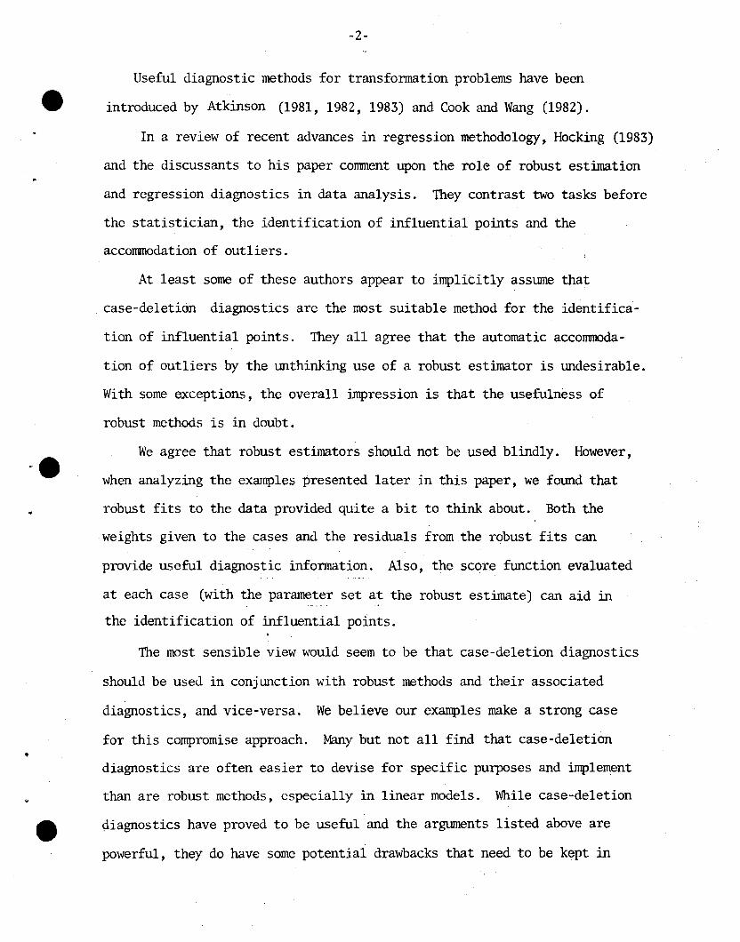
\\here the response diagnostic is
w . = ~(r.(~))/r.(~) .r,l 1 1
As we shall show in the examples, the estimate of >.., the design diagnostics,
the response diagnostics, and the residuals from the robust fit provide a
wealth of useful infonnation.
2.4 Bounded influence estimators. None of the estimators introduced so
far has a bounded influence function, though in the examples we have studied,
Schweppe-type estimators handle outliers reasonably well. A bounded
influence transfonnation [BIT(a)] estimator, depending on the constant a,
can be constructed by a method applicable for general parametric estimation
problems. The method is given by Stahel (1981) and has its origins in work
by Hampel (1968, 1974). Let 8 = (8,0,>") and let f(Yi,x i ;8) be the density
of yi given Xi \\hen 8 obtains. Denote the gradient of the log-likelihood by
£(y. ,x. ;8) = 'V8log fey. ,x. ;8). Now let A be a matrix solving1 1 1 1
(2.7)
\\here
(2.8)
-1 R 2 .tA = n 2 E {w (y,x. ;8) [£(y,x. ;8)] [R.(y,x. ;8)] },i=l Y 1 1 1
t -1 _1w(y,X;8) = min{l,av'p+2[(£(y,x;8) A (£(Y,x;8)] Z} ,
a > 1, and of course (p+2) is the munber of parameters being estimated. ThenA
8 solves
(2.9)n A ALw(y. ,x. ;8)[£(y. ,x. ;8)] = o.
. 1 1 1 1 11=
The matrix A is a robust version of the second moment matrix of £(y,x;8)
and (2.8) shows that the weights are based upon a Maha1anobis-type distance
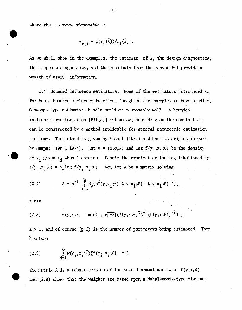
-10-
of t(y. ,x. ;8) from the centroid of U(y. ,x. ;8): i=l, ... ,nl. As a -+ co,1 1 1 1
w(Yi,Xi ;8) -+ 1 for all i and 8 converges to the MLE.
The influence function evaluated at (y.,x.) is1 1
A -1 A A
IF(y. ,x. ;8) = B w(y. ,x. ;8)t(y. ,x. ;8)·1111 ·11
where
-1 ~ Z A A t AB = n l. E {w (y,x.;8)t(y,x.;8)t (y,x.;8)} .i=l Y 1 1 1
The asymptotic covariance matrix of 6 is V = B-lAB-l . A measure of influence
motivated by Krasker and Welsch is
Yz = max[IF(y. ,x. ;8) tv-lIF(y. ,x. ;8)]! = max[t(y. ,x. ;6)tA- l t(y. ,x. ;8)]!ill 1 1 ill 1 1
Stahel (1981) calls YZ the self-standardized gross-error sensitivity.
"Self-standardized" refers to the fact that the influence flmction is being
normed by the estimator's own asymptotic covariance matrix. By the construc
.e tion of 8,
Yz ~ a.
Note that (ajas)t(y.,x.;8) is linear in E. but (ajaa)t(y.,x.;8) is quadratic1 1 111
in Ei . Thus as IEil -+ co, the weight w(Yi,xi ;8) goes to zero sufficiently
fast so that
w{y. ,x. ;8) II (ajaB)t(y. ,x. ;8) II -+ o.·1111
Therefore, as far as estimation of B is concerned, 8 is similar to regression
M-estimates with a "psi function" which redescends to 0, and we can expect
the BIT to be somewhat similar to the pseudo-MLE. For the regression problem,
this fact was noted by Hampel (1978).
Since (ajaA)t(y.,x. ;8) is a function of log(y.), if y. is either close to1 1 1 1
o or large, then the ith observation may have a high influence even if IEil
is small and x. has only small leverage. Among the estimators we consider,1
only the BIT bounds this source of influence. We define

-11-
which measures the downweighting of the ith observation due to this total
influence being large.
Both 8 and A were estimated by an iterative algorithm that was modeled
on the Krasker-Welsch algorithm of Peters, Samarov, and Welsch (1982).
'The weighting of .Q,(Yi,xi ;8) introduces a bias, which we suspect is
appreciable only for a. 'The bias could be removed (asymptotically) by
subtracting a suitably defined constant vector a from .Q,(y. ,x. ;8). However,1 1
a depends on 8 and we have not been able to find a convergent algorithm
for estimating a, 8, and A.
3. Confidence Intervals for A
Large-sample confidence intervals for A can be constructed using either
(i) the asymptotic normal distribution of (A-A) or (ii) modified likelihood- .
.e ratio tests.
Confidence intervals for Awere derived from likelihood-ratio tests in
the original paper of Box and Cox (1964). A modification of their method
is possible for thepseudo-MLE (or, more generally, when the estimator of
A is defined as the minimizer of a real-valued fmction). As discussed by
Carroll (1980, 1982), let Lmax(A) be the max~ over S and a of (2.2)
with A held fixed. To text HO: A=AO' we use the test statistic
where the correction factor

·e
-12-
N 2 N 2 2-1D = ( I ~(r./at.)~.w ./t.) ( I ~k(r./at.)~.w.) ,
i=1 1 1 1 X,l 1 i=1 1 1 1 X,l
is introduced so that T(AO) is asymptotically (as n ~ 00 and a ~ 0 simul
taneously) chi-square with 1 d.f. when HO holds. See Bickel and Dokstml
(1981) for an introduction to "small-a" asymptotics .. Also see Schrader and
Hettmansperger (1980) for a similar correction factor. The correction factor
is based on small-a theory, and we have found that this test will tend to
be conservative when the noise is large relative to the signal, as occurs
especially in the first example.
We saw no way to develop a likelihood-ratio-type test for BIT. But this
estimator is approximately normally distributed and its covariance matrix can
A and B are estimated by using expectation
with respect to the empirical distribution of (Yi'xi ) in the definitions of
A and B. For example.
A -1 N A "t "B= n I w(y.,X.;8)~(y.,x.;8)~ (y.,x.;8).
. 1 1 1 1 1 1 11=
4. Examples
4.1 Introductory remarks. In this section we will apply the following
estimators to three previously published data sets:
1) MLE = the maximum likelihood estimator
2) The pseudo-MLE of section 2.

-13-
3) BIT(l.s) = the bounded influence estimator with a = 1.5.
4) BIT(1.3) = the bounded influence estimator with a = 1.3.
When calculating the first two estimators and their confidence inter
val s, the parameter A was restricted to 1ie between -1.0 and +1.0. When
calculating BIT(l.s) and BIT(1.3), no restrictions were placed on A.
4.2 Salinity data. These data were obtained during collaboration
with members of the Curriculum in Marine Sciences at the University of North
Carolina and were used in Ruppert and Carroll (1980) to illustrate several
robust regression estimators. Atkinson (1983) used them to illustrate
regression diagnostics and power transformations. The response is salinity
or salt concentration (SAL) in North Carolina's Pamlico Sound measured
biweekly during the spring seasons of years 1972 through 1977. The explana
tory variables are salinity lagged by 2 weeks (SALLAG), TREND which is the
number of biweekly periods since the beginning of the spring season, and
the volume of river discharge into the sound (DSQ-IG). The data were a
minor part of a larger study aimed at predicting brown shrimp harvest.
The salinity data is a seemingly manageable, yet extremely complex, data
set. In the interest of clarity and for future researchers, it may be
worthwhile to describe the physical background of the data. Water salinity
SAL was measured at certain marshy areas located near the estuaries of the
major rivers which empty into Pamlico Sound; these areas were chosen because
this environment was thought to be of importance during the growth cycle of
brown shrimp. The physical structure suggests that the salinity measure
ments in the nursery areas will exhibit some autocorrelation within years,
and we found this correlation convenient to express through the lagged salinity
SALLAG. River discharge DSa-IG measures the volume of river water flowing
into the sound. Originally, it was thought that the higher the river flow,

-14-
the more fresh water would diffuse into the brown shrimp breeding grounds,
thus lowering salinity. Inspection of the data revealed periods of
very heavy discharge, see for example data points #5, #16. The marine
biologists working with us suggested that these large values of DSCHG
represented a real change in the system, in that at some point the
rivers would be flowing so fast that increases in DSCHGwould not lead- - .- -~ -
to much increased fresh water diffusion into the breeding areas, and hence
past some point the effect of increased DSCHG would be negligible or possibly
even vositive. We handled this phenomenon in an ad hoc fashion by
simply setting DSCHG equal to 26.0 whenever it actually exceeded 26.0.
In Ruppert and Carroll (1980), large DSCHG values were left unchanged
to obtain a data set with anomalous observations for testing robust
procedures. As we shall see, much of the problem with analyzing these
data can be traced to those points with recorded DSCHG L 26.0. A
linear time trend TREND was also added into the model because North
Carolina usually warms quickly in spring, which suggests possible
evaporation and increased salinity.
Incidentally, the salinity data analyzed here did not form a part
of the final prediction model used by the North Carolina Department
of Fisheries, although our experience gained in working with these data
was helpful. The final model, based on only· six years of data, was
used blindly but successfully by the Fisheries Department for four years,
1978-1981.
'lhere are an almost infinite variety of models which can be fit to
the salinity data. We shall study only two such models. When trans
forming the response SAL it seems sensible to simultaneously transform
the lagged response SALLAG. While we believe it is certainly permis
sible for illustrative purposes to consider models that only trans-

-15-
form the response SAL and not the lagged response, it is important to
4It keep in mind some reasonable alternatives.
The bivariate relationship between SAL and SALLAG is fairly linear with
no apparent outliers; see Figure 4.1. A scatter diagram (not shown here) of
SAL and TREND suggests a possible weak linear or quadratic relationship.
Figure 4.2 is a scatter diagram of the residual of SAL regressed on SALLAG
plotted against DSCHG. DSCHG is distributed with a noticeable positive
skewness. The rather linear relationship between these residuals and DSCHG
·e
when DSCHG is below about 26 seems to break down for larger values of DSCHG.
Observations #5 and #16 have IIUlch higher values of SAL than would be
expected if the linear relationship held across all values of DSCHG.
These observations also are high leverage points.
Observation #3 is also somewhat unusual. It has the third highest
value of DSCHG, very low values of SAL and SALLAG, and the lowest
possible value of TREND. However, in regard to the relationship between
SAL and SALLAG, TREND, and DSCHG, #3 does conform reasonably well with
the bulk of the data. In Figure 4.2 cases #9, #15 and #17 appear as some-
what outlying.
Atkinson (1983) uses these data to illustrate diagnostic methods.
He considers what we shall call the BASIC model, wherein a transfonned
value of water salinity SAL is regressed linearly on lagged salinity,
rlver discharge and TREND. He first modifies #16 from 33.443 to 23.443,
leading to ~ = 0.46. Using a "constructed variable", he flnds that
observation #3 is highly influential for estimating A, since after"'-
deleting it we obtain A = -0.15. With #16 corrected and #3 deleted,
Atkinson suggests the log transformation. The entire process is
effectively the same as having deleted both #3 and #16.

-16-
Despite the fact t:hat: the BASIC model does not transfonn the pre
dictor lagged salinity, we will illustrate our methods on this model so as
to compare them with Atkinson's. In Table 4.1 we exhibit details of
estimates and diagnostics. The pseudo-MLE suggests that it is #5 and
#16 which do not fit the data well, while #3 is an unusual design point;
in light of Atkinson's analysis, the emergence of #5 as possibly
influential strongly suggests masking. Somewhat more expected1y the BIT
methods identify #16 as an outlier with #3 and then #5 as possibili-
ties.
The results of our analysis indicate the possibility that the effect
of observation #S is being masked by #3 and #16. That this is the case
is illustrated by Table 4.2, where we array the various estimates of A
having deleted the COmbinations (3,16) (5,16) and (3,5,16). Observation
#5 is highly influential for the MLE of Aafter #3 and #16 are deleted.
This is classic case of masking, one of the better examples we have seen
with real data.
The Cook and Wang LD transformation d1agnostic 1S not immune to the
masking in #5. For the full data, their diagnostic clearly identifies
#3 and #16 as potential problems, but no hint: is given that #5 might be
unusual. After deleting #3 and #16, we recalculated the diagnostic, at
which point #~ becomes an obvious candidate for special treatment.
The analysis of the BASIC model shows that in using diagnostics
such as Atkinson's or Cook and Wang's to see if a point has a
potentially large impact on the MLE for the transfonnation parameter A,
the careful analyst must be concerned with masking and should recompute
the diagnostics after case de1et:ion. While we do not claim that our methods,
and especially our estimates, should be used blindly and will be immune
to masking, we do hope that this example illustrrates that robust methods

•
-17-
can provide valuable and non-redlUldant infonnation to the data analyst.
We' now tum to a model in which lagged salinity is also transfonned;
this is the TRANSFORMED model
(4.1) SAL(A) ; S + S SALLAG(A)+ S TREND + S DSCHGa 1 2 3'
As discussed previously, graphical methods and Figure 4.2 suggest that
it is #5 and #16 that are very lUlusua1, #9, #15, #17 somewhat less so,
and that in fact #3 conforms reasonably well with the bulk of the data.
To some extent this is confinned by the robust method analyses, which are
given in Table 4.3. Certainly #5, #16 are real outliers, but #3 appears to
fit the data reasonably well, although it is an lUlusua1 design point.
Observation #3 only becomes an outlier if one attempts to transfonn SAL
but not SALLAG.
At this point in time analogues to the LD diagnostic of Cook and Wang
have not been developed for the TRANSFORMED model (4.1), although it was
very easy to modify our programs to construct the robust estimates and
diagnostics for this new model. It is interestlng to study Table 4.3,
where observation #3 has an enonnous effect on the estimate of A only when
#5 is included in the model. This fact may serve as a test for future
diagnostics applied to model (4.1).
As stated at the outset, the salinity data are complex. For example,
we have performed residual analyses on each of the models presented
here, and the reader may wish to verify why we are not entirely satisfied
with the results. Other analyses may also be contemplated; we have used
our techniques on a model segmented at river discharge = 25, a model in
which lagged river discharge is used rather than simple river discharge,
and others. We have chosen the two models in this section not because
they are the best possible, but rather because they are simple and

-18-
illustrate that our robust estimates and diagnostics can be used as an
infonnative tool and not merely as a black box.
4.3 Stack loss data. This is an often analyzed data set; see among
others Brownlee (1965), Daniel and Wood (1980), Andrews (1974), Dempster
and Gasko-Green (1981). Observations 1, 3, 4. and 21 have been identi
fied as outliers by these authors, with the second and fourth authors
suggesting that observation 2 may also be outlying. Atkinson (1982)
fotmd that the MLE of A is 0.30 for the first order model in the three
explanatory variables with all observations included, while if. #21 is
excluded then the MLE is ~ = 0.48. Atkinson also considered a second
order model.
We have only considered the first order model. The robust esti
mators and their associated diagnostics are given in Table 4.4; the
estimators agree among themselves and with Atkinson that A about 1
is reasonable. The pseudo-MLE diagnostics indicatethatobserva
tions #2, #4 and #21 are not well fit by the model, with #1, #17 also
being tmusual design points. The BIT methods suggest that #2, #4
and #21 are very poorly fit by the model, and suggest that #3, #16 are
worth further investigation. If for each observation we evaluate the deri
vative of the log-likelihood with respect to A evaluated at the BIT (1.3)
estimate, then #2, #3, #4 and #21 stand out; their absolute values all
exceed 64.0, while no other exceeds 38.0.
The Cook and Wang LD diagnostic originally identifies #21 as possibly
interesting; although LD(#2l) is only about 0.70 it still stands out.
After removing #21, observation #16 now stands out, but LD(#16) is
extremely small being only about 0.25. We think it would be unusual to
continue the diagnostic-deletion process. At this point the diagnostic
process would probably delete #21, take A = 1 and begin ordinary regression

. ~
·e
-19-
diagnostic-deletion.
All the methods identified #21 as having the biggest potential for
trouble. The methods we have introduced also identify potential diffi
culties with #2, #3 and #4. Faced with the conclusion that at least 4
of 21 data points do not fit a model, the analyst might reasonably question
either the model or the data. One could attempt to accommodate the first
4 data points by changing the model, as many previous authors have done
by suggesting "second order" models. Alternatively, following Daniel and
Wood, one might question whether the first 4 observations are really
valid data points.
We believe that for the first order model in the stack loss data,
the robust estimates and diagnostics we have introduced provide valuable
information. Combining previous d1agnostics with our methods appears to
have been quite successful.
4.4 Artificial data of Cook and Wang. This is an eleven
case data set created by Cook and Wang (1983). These artificial data have
the property that the model log y. = x.+s. fits the first ten cases, but111
the model Ey = BO+Blx f1ts the complete data. Cook and Wang's LD
diagnostic identifies #11 as particularly influential, because it is
unusual in both the design and the response.
The various estimates of the transformation parameter A are repro-
duced in Table (4.5), both with and without Case #11. Clearly, Lhe MLE is
dramatically affected by #11, as are the BIT estimates. The pseudo-MLE
method downweights #11 sufflciently as to effectively exclude it from the
analysis. The fact that the pseudo-MLt aULomatically downweighLs any
unusual d.eslgn point is the property which makes it an effective esti-
mat ion technique in this example.

-20-
The pseudo-MLE and BIT methods also contaIn useful dwgnostlc infotm1-
e tion..An index plot or simply the mnnbers listed for the complete data
tell us through the BIT methods that both #10 and HI are potentially
interesting, since the other nine case weights equal one. The pseudo-MLE
suggests that Doth #lu and #11 are unusual design points, but that #11
is a response outlier as well. The reduced data analyses support This
conclusion.
COOK and Wang conclude their analysis after deleting #11, having
noted that when applied to the complete daTa their LD diagnostic identi
fies only #11 as potentially interesting. Of course, they have the
somewhat unusual advantage of knowing the model which is intended
to fit the data. In practice we would be faced with the problem of
whether to repeat The diagnostic process. .tlecause of the potential for
masking found in the salinity data, for illustratlve purposes we repeaTed
the COOK and Wang dlagnostic analysis on the reduced data set, without #11.
For the reduced data without #11, the Cook and Wang 10 dlagnosTic
strongly suggests further study of #10, since LD(#lO) ; 3.3 and all other
LD statistics are below 1. 2. There is a potential masking effect here in
the LD statistics: #10 was not seen to be potentially influential for the
complete data set. If we were to delete #10 as well as #11, the MLE
becomes ~ = 0.15 with an associated 95% confidence interval which
includes [-1.0, 1.0]. In combination with the BIT and pseudo-MLE
analyses, the last confidence interval suggests that #11 is a design and
response outlier, while #10 is a somewhat unusual design point that
contains information about the transformation parameter A.
It is probably not useful to draw too strong a conclusion from a
small, specially constructed artificial data set. It seems clear from
this example that no single method will suffice. It seems most sensible to

-21-
combine the infonnation given from robust estimates, their associated
diagnostics, specially constructed diagnostics such as Cook and Wang's LD
statistic, and standard procedures such as the confidence intervals.
5. Conclusions
The classic work is robust estimation dealt with location parameters
and was concerned with heavy-tailed deviations from the nonnal distribution.
Earlier work on robust regression, e.g. Huber (1973), also concentrated on
distributional robustness. However, regression models are at best only
approximately correct, and they easily can break down at the extreme points
of the factor space. Therefore, it was natural that techniques, such as
the Krasker-Welsch (1982) estimator, that bound the influence of such points
would be developed for linear models.
The use of transfonnations is a power~ul technique for model building,
since transformed data will often fit a simpler model than the raw data.
As when using standard (untransformed) regression models, here too, one
needs to guard against the possibility that one or a few extreme points in
the factor space will overwhelmingly affect the data analysis, especially
the choice of a transfonnation.
We have introduced several estimation techniques for the Box-Cox (1964)
transfonnation model that, unlike the MLE, are relatively insensitive to
outliers in both the design and in the residual. In several examples, these
estimators proved valuable not only at the final estimation stage of the
analysis, but also at the preliminary model identification stage. For
model selection purposes, the robust estimators should be viewed as useful
supplements to the diagnostic techniques of Atkinson (1982, 1983) and
Cook and Wang (1983).

-22-
MOdel selection, the identification of outliers, and the choosing of a
transformation must be done simultaneously. Also, the masking of some
outliers by other outliers is a potential problem. For these reasonS, at
least, diagnostic information from as many sources as feasible should be
used.

·e
REFERENCES
ANDREWS, D.F. (1974). A robust method for multiple linear regression.Technometrics, 16, 5?3-531. ._- .... .
ATKINSON, A.C.. (1981) ..Two graphical displays for outlying and influentialobservations in regression. Biometrika, 68. 13-20.
ATKINSON, A.C. (1982). Regression diagnostics, transformations and constructed variables (with discussion). JRSS-B, 44, 1-36.
ATKINSON, A.C. (1983). Diagnostic regression analysis and shifted powertransformations. Technometrics, ~i, 23-33.
BELSLEY, D.A., KUH, E., and lVELSCH, R.E. (1980). Regression Diagnostics.New York: Wiley.
BICKEL, P.J., and OOKSUM, K.A. (1981). .An analysis of transformationrevisited. J. Am. Statist. Assoc., 76, 296-311
BOX, G.E.P. and COX, D.R. (1964). .An analysis of transfonnations (withdiscussion). J. Roy. Statist. Soc., Ser. B, 26, 211-246. .
BROl~LEE, K.A. (1965). Statistical Theory and Methodology in Scienceand Engineering. New York: Wiley.
CARROLL, R.J. (1980)~ A robust method for testing transfonnations toachieve approximate normality. J. Roy. Statist. Soc., Series B,. 42, 71-78 ..
CARROLL, R.J. (1982). Two examples of transformations when there arepossible outliers. Applied Statistics, 31, 149-152.
COOK, R.D. and WANG, P.C. (1983). Transformation and influential casesin regression. Technometrics,~, 337-343.
COOK, R.D. and WEISBERG, S. (1982). Residuals and Influence in Regression.New York and London. Chapman and RaH.
DANIEL, C. and WOOD, F.S. (1980). Fitting Equations to Data, 2nd Edition.New York: Wiley.
Dfl-.1PSTER, A.P., and GASKO-GREEN, M. (1981). New tools for residualanalysis. Ann. Statist., ~, 945-959.
HAMPEL, F.R. (1968). Contributions to the TheOik of Robust Estimation.Ph.D. Thesis. University of California, Ber e1ey.
HAMPEL, F.R. (1974). The influence curve and its role in robust estimation.J. Amer. Statist. Assoc., 62. 1179-1186.

HAMPEL, F.R. (1978). Optimally bounding the gross-error-sensitivity and theinfluence of position in factor space. 1978 Proceedin~s of the ASAStatistical Computing Section. ASA, Washington, D.C., 59-64.
HOCKING, R.R. (1983). Developments in linear regression methodology:1959-1982 (with discussion). Technometrics, 25, 219-249.
HUBER, P.J. (1964). Robust estimation of a location parameter. Ann. Math.Statist., 35, 73-101.
HUBER, P.J. (1973). Robust regression: asymptotics, conjectures andMOnte Carlo. Ann. Statist., ~, 799-821.
HUBER, P.J. (1983). Minimax Aspects of bounded-influence regression.J. Am. Statist. Assoc., 78,66-80.
KRASKER, W.S. (1980). Estimation in linear regression models withdisparate data points. Econometrica, 48, 1333-1346.
KRASKER, W.S. and WELSCH, R.E. (1982). Efficient bounded-influenceregression estimation. J. Am. Statist. Assoc., 77, 595-604.
PETERS, S.C., SAMAROV, A.M., aIld WELSCH, R.E. (1982). Computationalprocedures for bounded-influence and robust regress"ion. Center forComputational Research in Economics and Management Science. Alfred P.Sloan School of Management Science. MIT.
RUPPERT, D. and CARROLL, R.J. (1980). Trimmed least squares estimation inthe linear model. J. Am. Statist. Assoc., ~, 828-838.
SCHRADER, R.M. and HETIMANSPERGER, T.P. (1980). Robust analysis of variancebased upon a likelihood-ratio criterion. Biometrika, 67, 93-10l.
SNEE, R.D. (1983). Discussion of "Developments .in linear regressionmethodology: 1959-1982" by R.R. Hocking. Technometrics, 25, 230-237.
STAHEL, W. A. (1981). _R_ob-;u~s_t..:..e_ST-c_ha-..:..e..:..t.,...zun.........-~e_n_:--..I.....n_f....in..:..i-;:t..,.e..:..s..:..ima~l_e..,....,.'-t_i_ma--.,...ll_· t....a_e..;..tund Schaetzungenvon Kovarlanzmatrlzen. .D. Dlssertatl0n. SwissFederal Institute of Technology, Zurich.

Table 4.1 Analysis of transformations for the BASIC salinity modelusing all the data. The 95% confidence intervals andstandard errors are as described in the text, as are thecase weights.
Weights for Selected CasesMethod Estimate 95% Standard
of A C.l. Error 113 liS 119 #15 1116 1117
MLE 0.97 (0.17,1.00) 0.75
Pseudo-MLE 0.69 (-0. ~4,1.00) Residual 1.00 0.00 0.82 0.55 0.00 0.71Design 0.40 0.09 0.72 1.00 0.02 1.00
BIT(1. 5) 0.51 0.36 0.43 0.51 0.46 0.55 0.04 0.89
BIT(1. 3) 0.51 0.27 0.17 0.24 0.28 0.26 0.03 0.46~e

Table 4.2 Analysis of transfonnations for the TRANSFORMED salinitymodel (4.1) us ing all the data. Note here that bothsalinity and lagged salinity are transformed.
Weights for Selected CasesMethod Estimate 95% Standard
of A C. I. Error #3 #5 #9 #15 #16 #17
MLE 0.66 (-0.16,1.00) 0.46
Pseudo-MLE 1.00 (-0.72,1. 00) Residual 1.00 0.00 0.84 0.52 0.00 0.69Design 0.40 0.09 0.72 1.00 0.02 1.00
BIT(1. 5) 0.94 0.41 1.00 0.33 0.42 0.42 0.06 0.53·eBIT(1.3) 1.06 0.41 0~95 f() .14 0,30 0.23 0.03 0.33

Table 4.3 Estimates of A for selected observations excluded. TheBASIC and TRANSFORMED models are described in the text;the latter transforms the predictor lagged salinity,while the fonner does not.
K)DEL
Estimator BASIC TRANSFORMED
Observations None 16 3,16 5,16 3,5,16 None 16 3,16 5,16 3,5,16deleted
MLE .97 .46 -.15 .70 .39 .66 .50 .22 1.0 1.0
Pseudo-MLE .69 .71 .22 .79 .40 1.0 1.0 1.0 1.0 1.0
·e BIT(1.3) .51 .50 .25 .80 .45 1.06 1.09 1.06 1.16 1.19

Table 4.4 Estimates of A for the complete stack10ss data. A firstorder model was used.
Weights rOT Selected Cases
Method Estimate 95% Standard#1 112 fJ3 1#4 '#21of A C.L Error
MLE 0.30 (-0.18,0.74) 0.38
Pseudo-t-n..E 0.49 (0.13,0.74) Residual 1.00 0.17 1.00 0.06 0.00Design 0;50 0.45 1.00 1.00 0.72
BITe!. 5) 0.39 0.29 1.00 0.72 1.00 0.47 0.27
BIT(1. 3) 0.41 0.23 1.00 0.37 0.88 0.25 0.13,e

Table 4.5 Estimates of A for the Data of Cook and Wang.
A
Estimator A 95% CI SE Weights for Selected Cases
no #11
Complete Data
MLE 0.71 (0.04,1.00)
Pseudo-MLE -0.14 (-0.66,0.88) 1.00 Residual 0.000.39 Design 0.01
BIT(1.3) 0.49 0.30 0.31 0.21
Reduced Data (Case #11 Excluded)Je MLE -0.18 (-1.00,0.57)
Pseudo-MLE -0.25 (-O. 72 ,0.86) 1.00 Residual0.23 Design .
BITe1. 3) -0.34 0.90 1.00

•List of Figures
Figure 4.1 Scatter diagram of salinity against lagged salinity withselected cases identified.
Figure 4.2 Scatter diagram of salinity residuals against dischargewith selected cases identified. Salinity residual isthe residual of salinity regres~ed on lagged salinity.

•
11
15
• •• ·23
1~ • •9 •• ••..
..11
S ..It .. .. ·15L 16]N
Je I ..1'I 9
•.. .. ·17
1
.. 6
"4
5 ·5
"3
~ 5
Figure 4.1
1 9 11
lilOOED SAL1N1TY
1'3 15 11

3•.5
•3. D
• 9
2. .5
-'2 •.5.15
-'3. 0 "17
-'3.5c
'2'2 '2'3 '2t '25 '21 '3'20 '21 '2"- '28 '2.9 '30 '31 '3'2 '3'3 '3t
e Figure 4.2 D1S CHAR GE