Embed Size (px)
Citation preview
Transfers within the Extended Family:
Theory and Evidence from South Africa
Olivier Donni∗
Eliane El Badaoui†
(November 2009)
Abstract
In this paper, we provide a theoretical framework for examining labor supply in
extended families. The labor supply is discrete and the self-selection of families
into the nuclear or extended household structures is endogenous to labor force
participation. We take into account the size of scale economies in consumption
and the monetary transfers within the extended household. The main structural
components of the model are shown to be identifiable. The model is then estimated
using South African data from the 1997 OHS.
JEL Classification: D13; J12; J22; O12
Key-words: Extended Family, Monetary Transfers, Labor Supply.
∗THEMA - Universite de Cergy-Pontoise, 33 Boulevard du Port, 95011 Cergy-Pontoise, France.E-mail: [email protected].†THEMA - Universite de Cergy-Pontoise, 33 Boulevard du Port, 95011 Cergy-Pontoise, France.
E-mail: [email protected].

1 Introduction
It is not uncommon, in many developing countries, to find several adults, couples or
families living together and sharing their resources. The extended household structure,
often considered as the core source of income insurance, affects the incentives to work
of household members.1 More specifically, if income sharing is prevalent in extended
households then economic policies may produce unexpected outcomes. Therefore, in
countries where various possible combinations of families exist, a specific analysis of la-
bor force participation allowing for money transfers within family is critical for assessing
the incidence of economic and social policies.
The influence of a large-size family on the behavior of household members incorpo-
rates special features. Importantly, the extended household structure may improve the
alternatives for child care arrangements since persons other than the mother may as-
sume child care responsibilities, freeing the mother for a labor market activity (Berhman
and Wolfe, 1984). Given that economies of scale depress the shadow price of consump-
tion, workers in extended families may be encouraged to modify their labor market
participation in favor of leisure, taking into consideration the labor market states of
the other members of the household.2 Kochar (2000) finds, for instance, that sons
contribute to household public goods such as consumer durables and ceremonial ex-
penditures enabling their father to work less. Foster and Rosenzweig (2002) estimate a
collective model of household division and find that gains from coresidence arise from
cost-sharing a household-specific public good and lower barriers to information-sharing
on farming techniques. The existence of scale economies in production makes desirable
the coresidence. Thus the consumption of public goods and the increasing returns in
household production make larger the optimal household size - which is typically the
case of households in poor rural economies (Lanjouw and Ravallion, 1995; Deaton and
Paxson, 1998; Fafchamps and Quisumbing, 2003). Given the monitoring advantages
of the household, cash and in-kind transfers within the extended family are expected
to be larger when members live under the same roof than when they live in different
housing. These transfers may, in turn, have a disincentive effect on workforce partic-1An extended household is “a household unit including any family members outside the core nuclear
family unit” (Angel and Tienda, 1982).2Technically, a decrease in the price of consumption will negatively affect the participation rate only
if the income effect prevails over the substitution effect.
2

ipation (Bertrand et al., 2003). Lastly, multi-person households are often thought to
affect negatively the participation rate because of a self-selection process of household
members. If adult’s membership in household results from a rational choice, then the
household structure is not exogenously taken. In fact, extended households may group
together individuals with low resources - or low taste for effort - who choose to remain
with their parents, children or married siblings.
In this paper, we develop an empirical model of labor supply taking into account
the sharing of resources among persons living in the household, and the economies
of scale in consumption. While the decisions in nuclear families are described by the
unitary approach, the decisions in extended families are Pareto-optimal and represented
by an income sharing rule. We assume a Barten type technology function so that,
due to economies of scale, the price of consumption is lower in the extended family.
The constitution of an extended family is endogenous to the discrete labor supply
decisions. In the first step, each family composed of a single or a couple decides whether
to constitute an extended family or not. This decision is endogenous to labor force
participation in that it is likely determined by the size of scale economies and the
families’ taste for consumption. In the second step, each single or couple living in an
extended family decides, taking into account the monetary transfers of the other persons
living under the same roof, whether to participate in the labor market on a full-time
basis or to stay out of it. We show that this model is completely identified from a sample
of singles, couples and extended families. In particular, the rule that determines the
distribution of resources between families and a measure of scale economies can be
recovered. We then apply this model to South African micro-data.
The identification strategy is inspired from the work of Gronau (1991), Couprie
(2007), Browning et al. (2008), and Lewbel and Pendakur (2009). The extended
family household is composed of nuclear families, the utility functions of which can be
recovered from the observation of the participation decisions of nuclear families living
alone - supposing that the utility function of a nuclear family is the same whether it
lives alone or with another family. The observation of the decision to participate in the
labor market of persons living in extended family households allows us to identify the
economies of scale and the levels of internal income transfers.
3

Structural models of family labor supply remain scarce about some important fea-
tures relative to developing countries among which the presence of multi-person house-
holds.3 In the empirical application of this paper, we use data from South Africa, a
country whose labor market is traditionally characterized by a significantly high level of
unemployment.4 The specificities of the South African labor market, together with the
availability and the quality of the data, have attracted attention from the profession.
In particular, studies by Case and Deaton (1998), Duflo (2000, 2003), and Bertrand
et al. (2003) using the Old Age Pension program, have discovered the existence of
bargaining within the extended family. These authors have also pointed out money
transfers from older to younger that affect younger’s decisions to participate in the
labor market. In the nuclear family, Quisumbing and Maluccio (2003) examine the in-
trahousehold allocation of resources between husband and wife and show that the share
of budget devoted to children’s education increases more with wife’s assets brought at
marriage than with husband’s. Like the labor market, the family structure in South
Africa displays some important features. In fact, the size and structure of households
have undergone dramatic changes over the last decade (Wittenberg and Collinson, 2005;
Pirouz, 2005). One of the main drivers of population growth dynamics and household
structure changes among South African population is the HIV/AIDS. South Africa has
more people with HIV/AIDS than any other country in the world. The virus plays a
major role in reshaping households and constitutes a critical source of changes in labor
supply in the country (see for instance, Thirumurthy et al., 2008).
The remainder of this paper is structured as follows. The theoretical model is
developed in the next section. Section 3 formulates parametric and non-parametric
identification. South African micro-data used in the empirical analysis are presented
in section 4. In section 5, we expose the empirical estimation and report the results of
the structural model. Section 6 concludes.3The studies of Newman and Gertler (1994) on rural landholding households in Peru, and Gong and
van Soest (2002) on the labor supply of married women in Mexico City remain to note.4Note that despite the high level of unemployment, the informal sector remains relatively small
compared to other countries in Sub Saharan Africa, Latin America, and Asia (even if it shows growthduring the recent years).
4
2 The Theoretical Model
In this section, we consider a very simple model with two types of households: nuclear
family households and extended family households. The nuclear household is defined
as either a single adult or a married couple - with or without children. The extended
household consists of two nuclear families living together. We first examine how the
participation in the labor market of nuclear and extended family households is decided,
and then discuss the factors that affect the decision of families to cohabitate.
In the remainder of this paper, we shall use the following notational conventions:
each couple and single family is indexed by i or j ∈ N ≡ a sample of single and couple
families; the extended families that include two couple families, two single families or
a couple family and a single family are then characterized by two indices i and j. The
structure of the nuclear family is described by an index r or s, where r/s = 1 for
single families and r/s = 2 for couple families (i.e., the index can be interpreted as the
number of adults in the family). The individuals are constrained on the labor market
so that only full-time jobs are offered to workers; hence working time of each person can
take only two distinct values. The number of alternatives offered to a nuclear family of
structure r is simply equal to 2r, and that offered to an extended family of structures
r and s is equal to 2r+s. The alternatives of a nuclear family are indexed by k or
l ∈ {1, . . . , 2r}.
2.1 The Behavior of Nuclear Families
To begin with we consider a nuclear family consisting of a single adult or a married
couple (with or without children) who make decisions about leisure and consumption.
The quantity of goods consumed in a family i choosing alternative k is denoted by cik.
The utility obtained by family i of structure r from alternative k is then equal to:
urik = γrk(zi) + βrk(zi) ·(cik)ρ
ρ(1)
where ρ is a parameter comprised between zero and one,5 βrk(zi) and γrk(zi) are functions
depending on the selected alternative and the structure of the family and zi is a vector5These restrictions on the values of ρ are not necessary. However, they make the interpretation
easier.
5
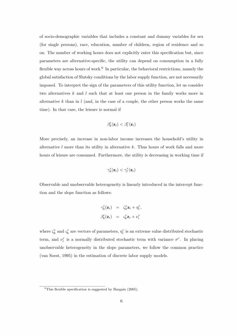
of socio-demographic variables that includes a constant and dummy variables for sex
(for single persons), race, education, number of children, region of residence and so
on. The number of working hours does not explicitly enter this specification but, since
parameters are alternative-specific, the utility can depend on consumption in a fully
flexible way across hours of work.6 In particular, the behavioral restrictions, namely the
global satisfaction of Slutsky conditions by the labor supply function, are not necessarily
imposed. To interpret the sign of the parameters of this utility function, let us consider
two alternatives k and l such that at least one person in the family works more in
alternative k than in l (and, in the case of a couple, the other person works the same
time). In that case, the leisure is normal if
βrk(zi) < βrl (zi)
More precisely, an increase in non-labor income increases the household’s utility in
alternative l more than its utility in alternative k. Thus hours of work falls and more
hours of leisure are consumed. Furthermore, the utility is decreasing in working time if
γrk(zi) < γrl (zi)
Observable and unobservable heterogeneity is linearly introduced in the intercept func-
tion and the slope function as follows:
γrk(zi) = ζrkzi + ηri ,
βrk(zi) = ςrkzi + νri
where ζrk and ςrk are vectors of parameters, ηri is an extreme value distributed stochastic
term, and νri is a normally distributed stochastic term with variance σr. In placing
unobservable heterogeneity in the slope parameters, we follow the common practice
(van Soest, 1995) in the estimation of discrete labor supply models.
6This flexible specification is suggested by Bargain (2005).
6

If there is no income transfer between families, the budget constraint for a nuclear
family i who chooses alternative k is given by:
cik = yi + eik
where eik is the labor income of family i for alternative k and yi is its non-labor
income. Typically, if taxation can be ignored, the labor income is simply defined by
eik =∑
awiahka, where the summation is made over adults a in family i, wia is the
wage rate of adult a and hka is her working hours in alternative k. To show how families
make decisions, we incorporate the budget constraint in the utility function and obtain:
urik = γrk(zi) + βrk(zi) ·(yi + eik)ρ
ρ(2)
The family is then facing 2r alternatives and selects the alternative k∗ that yields the
highest level of utility, that is,
urik∗ = maxk∈{1,...,2r}
urik
One remark is in order here. To make the model as simple as possible, and limit
the number of parameters to estimate, we suppose that the behavior of couples is
consistent with the unitary approach, i.e., the household behaves as a single agent.
The unitary approach can be seen as a reduced-form of the true decision process here;
of course, it does not mean that there is no economies of scale and income distribution
between spouses, but simply that our concern is what happens within the extended
family and not the nuclear families. Note that the unitary representation of spouses’
behavior is not really restrictive here because neither the Slutsky symmetry nor the
negativity are imposed in our model.7 In principle, it would be possible to model
the behavior of couple families by the collective approach, thereby supposing that the
distribution of bargaining power within the family depends on spouses’ wage rates and
some other variables. However, the identification of the “individual” utility functions
may be complicated in practice. Indeed, in the empirical application, we opt for a7The only restriction we impose is the exclusion of distribution factors. However, the empirical
application does not use distribution factors.
7
strategy of identification that exploits a comparison of nuclear families and extended
families. To do so, we need valid instruments to explain the participation to a specific
form of family that we do not have to model the decision of marriage.8
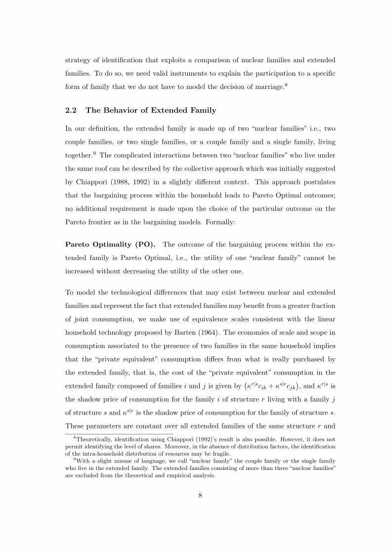
2.2 The Behavior of Extended Family
In our definition, the extended family is made up of two “nuclear families” i.e., two
couple families, or two single families, or a couple family and a single family, living
together.9 The complicated interactions between two “nuclear families” who live under
the same roof can be described by the collective approach which was initially suggested
by Chiappori (1988, 1992) in a slightly different context. This approach postulates
that the bargaining process within the household leads to Pareto Optimal outcomes;
no additional requirement is made upon the choice of the particular outcome on the
Pareto frontier as in the bargaining models. Formally:
Pareto Optimality (PO). The outcome of the bargaining process within the ex-
tended family is Pareto Optimal, i.e., the utility of one “nuclear family” cannot be
increased without decreasing the utility of the other one.
To model the technological differences that may exist between nuclear and extended
families and represent the fact that extended families may benefit from a greater fraction
of joint consumption, we make use of equivalence scales consistent with the linear
household technology proposed by Barten (1964). The economies of scale and scope in
consumption associated to the presence of two families in the same household implies
that the “private equivalent” consumption differs from what is really purchased by
the extended family, that is, the cost of the “private equivalent” consumption in the
extended family composed of families i and j is given by(κr|scik + κs|rcjk
), and κr|s is
the shadow price of consumption for the family i of structure r living with a family j
of structure s and κs|r is the shadow price of consumption for the family of structure s.
These parameters are constant over all extended families of the same structure r and8Theoretically, identification using Chiappori (1992)’s result is also possible. However, it does not
permit identifying the level of shares. Moreover, in the absence of distribution factors, the identificationof the intra-household distribution of resources may be fragile.
9With a slight misuse of language, we call “nuclear family” the couple family or the single familywho live in the extended family. The extended families consisting of more than three “nuclear families”are excluded from the theoretical and empirical analysis.
8

s. The budget constraint is then given by:
κr|scik + κs|rcjk = yi + yj + eik + ejk
If the shadow price of consumption is below one, then there are economies of scale.
Hereinafter, we illustrate how the shadow price are determined.
In the present framework, where all the consumption is equivalently private, the PO
hypothesis essentially means, as explained by Chiappori and Ekeland (2006, 2009),
that there exists a well-behaved rule that determines the sharing of total non-labor
income between the two “nuclear families”. In a first step, the total non-labor income is
allocated between families according to the so-called sharing rule, so that the family i of
structure r cohabitating with family j of structure s receives a share of total non-labor
income equal to φr|s(xi,xj), with
φr|s(xi,xj) + φs|r(xj ,xi) = yi + yj ,
where xi and xj are vectors of variables that influence the distribution of resources
within the extended family. In a second step, each family maximizes its utility with
respect to its budget constraint. The second-stage budget constraint of family i can
thus be written as:
κr|scik = φr|s(xi,xj) + eik.
Thus, the extended household budget constraint can be written:
κr|scik + κs|rcjk = φr|s(xi,xj) + φs|r(xj ,xi) + eik + ejk
In order to interpret scale economies in consumption, let us suppose that the fraction
of joint consumption in a family of structure r living with a family of structure s is
constant and equal to θr|s, and the fraction of private consumption is equal to 1− θr|s.
The consumption of the nuclear family who cohabitates is then equal to:
cik = φr|s(xi,xj) + eik + θs|r[φs|r(xj ,xi) + ejk];
9

By assuming that the consumption values are equal for the two nuclear families, that
is φs|r(xj ,xi) + ejk = φr|s(xi,xj) + eik,
cik = (1 + θr|s)[φr|s(xj ,xi) + eik];
hence, κr|s = 1/(1 + θr|s) and, similarly, we have: κs|r = 1/(1 + θs|r). Note that the
fraction devoted to private consumption certainly depends on the number of persons
living in the nuclear family i. Therefore, the economies of scale that can be exploited
from the extension of the family are likely more limited for a couple family than for a
single family.
If we incorporate the corresponding budget constraint in the utility function of
family i, we obtain:
urij = γrk(zi) +βrk(zi)ρ·(φr|s(xi,xj) + eik
κr|s)ρ (3)
The extended family then selects the alternative k that maximizes this function.
To make things easier, we suppose here that the sharing rule is everywhere continu-
ous, thereby implying that an extension of the “double indifference” condition, due to
Blundell et al. (2007), is satisfied. This condition says, more precisely, the following.
Double Indifference (DI). The utility of one “nuclear family” along the participa-
tion frontier does not depend on the participation decisions of the other one.
The DI hypothesis intuitively means that the drop in leisure, when one person in the
extended family is participating, is compensated exactly by a discontinuous increase
in consumption of this person that preserves the smoothness of each family’s well-
being.10 Technically, a consequence of DI is that the share received by family i is not
indexed by the alternative k chosen by the family j (and conversely) This condition is a
real assumption, albeit not extremely restrictive: the fact that both “nuclear families”
should be indifferent sounds like a natural requirement, especially in a context where
compensations are easy to achieve via transfers of the consumption good.10Note that PO requires that, if one “nuclear family” is indifferent between participating along the
frontier, then the other one is indifferent as well.
10
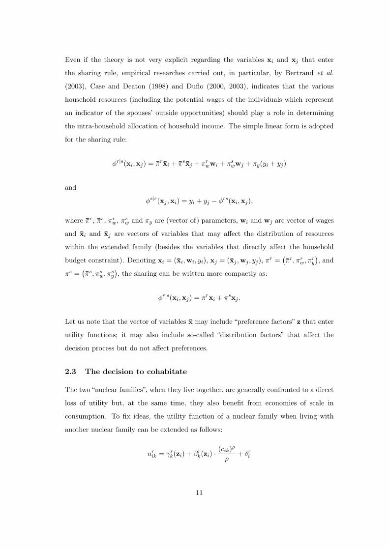
Even if the theory is not very explicit regarding the variables xi and xj that enter
the sharing rule, empirical researches carried out, in particular, by Bertrand et al.
(2003), Case and Deaton (1998) and Duflo (2000, 2003), indicates that the various
household resources (including the potential wages of the individuals which represent
an indicator of the spouses’ outside opportunities) should play a role in determining
the intra-household allocation of household income. The simple linear form is adopted
for the sharing rule:
φr|s(xi,xj) = πrxi + πsxj + πrwwi + πswwj + πy(yi + yj)
and
φs|r(xj ,xi) = yi + yj − φrs(xi,xj),
where πr, πs, πrw, πsw and πy are (vector of) parameters, wi and wj are vector of wages
and xi and xj are vectors of variables that may affect the distribution of resources
within the extended family (besides the variables that directly affect the household
budget constraint). Denoting xi = (xi,wi, yi), xj = (xj ,wj , yj), πr =(πr, πrw, π
ry
), and
πs =(πs, πsw, π
sy
), the sharing can be written more compactly as:
φr|s(xi,xj) = πrxi + πsxj .
Let us note that the vector of variables x may include “preference factors” z that enter
utility functions; it may also include so-called “distribution factors” that affect the
decision process but do not affect preferences.
2.3 The decision to cohabitate
The two “nuclear families”, when they live together, are generally confronted to a direct
loss of utility but, at the same time, they also benefit from economies of scale in
consumption. To fix ideas, the utility function of a nuclear family when living with
another nuclear family can be extended as follows:
urik = γrk(zi) + βrk(zi) ·(cik)ρ
ρ+ δri
11

where δri is a positive constant if cohabitating generates direct advantage in terms of
utility (besides economies of scale and transfers) and a negative constant otherwise.
The optimal decision will result from the trade-off between these advantages and dis-
advantages. If the decision to cohabitate is Pareto-Optimal, then the two generations
will decide to live together on the condition that cohabitating generates a global pos-
itive surplus. The surplus will depend, in particular, on the disagreement associated
to cohabitation for each “nuclear family” and on the income available for each “nuclear
family”, i.e., the “nuclear family” will “buy” the possibility to live alone if the income is
sufficiently important. The surplus will also depend on the specific taste for consump-
tion of each “nuclear family” and on the economies of scale in consumption. The idea is
that, if both “nuclear families” attach importance to consumption, then they will more
easily accept to support the desutility of living together to benefit from economies of
scale.
The decision to cohabitate is even more complicated because it depends on the com-
plete environment of the household. For instance, the existence of several children and
of several parents makes that the negotiation cannot be seen as simply bilateral. A
structural approach then requires to construct a matching model (a la Gale) between
a large number of agents, which is largely beyond the scope of this paper (see Brock
and Durlauf (2001) for a survey of this literature). In the empirical section, we thus
opt for a reduced-form equation for the self-selection into the extended family. From
the discussion that precedes, it must be clear that the error term of this equation will
generally be correlated with the heterogeneity terms νsi . It is reasonable to suppose
that nuclear families that decide to cohabitate have a marked taste for consumption.
3 Identification
We first examine how the parameters can be identified from a sample of nuclear and
extended families. The procedure can be then generalized to a non-parametric identi-
fication.
If, in a first step, the selection problem is ignored, it is clear that the previous
model is (parametrically) identified. As in any mixed logit model, the absolute level
of utility is irrelevant; only difference in utilities can be identified (see Train, 2003, for
12

instance). Hence, the intercept function γrk(zi) must be normalized for one alternative.
For instance, without loss of generality, we use the following identifying restriction:
γrk(zi) = 0, hence ζrk = 0 for k = 1.
In that case, the vector of parameters ζrk for k = 2, . . . , 2r and ςrk for k = 1, . . . , 2r and
r = 1, 2 can be recovered from a sample of single families and nuclear families.
Let us recall that, in an extended family, the utility function for the family i of
structure r can be written as:
urik = γrk(zi) +βrk(zi)ρ·(φr|s(xi,xj) + eik
κr|s)ρ.
The idea of the identification strategy is that, knowing the parameters ζrk and ςrk as well
as α, the sample of extended families will allow one to identify the other parameters
κr|s, κs|r, πr and πs. Instead of formally demonstrating this result, which is rather
intricate, we can give here the intuition. Let us consider two families i and i′ with
exactly the same characteristics z∗i and w∗i , the former is living in an extended family
and the latter in a nuclear family. If the families i and i′ have the same probability
to choose alternative k, then they must have the same level of consumption and, in
particular,φr|s(xi,xj) + eik
κr|s= yi′ + ei′k (4)
This gives one equation. In order to identify (φr|s, φs|r) and (κr|s, κs|r), the observation
of the participation decision of two other persons living in the extended family can
be used11 and generate a second and a third equation. Solving these equations, and
noting that φr|s(xi,xj) + φs|r(xj ,xi) = yi + yj , then gives (φr|s, φs|r) and (κr|s, κs|r).
Interestingly, this intuition remains valid in a non-parametric context provided that
φr|s and κr|s are not stochastic.
The crucial feature in the preceding discussion is the possibility to deal with the
selection problem. To do so, the presence of a regressor that traces out the probability
of selection is necessary. Intuitively, if there exists a set of instruments, independent of11Alternatively, the probabilities can be computed at a different point z∗∗i and w∗∗i . This gives other
equations.
13

families’ participation decisions, with some configuration such that the probability of
living in a nuclear family is equal to one, then the parameter α and the functions βrk(zi)
and γrk(zi) can be identified. If the probability of living in a nuclear family is equal to
zero for another configuration of the instruments, then the other structural components
of the model, the parameter κr|s and the function φr|s(xi,xj) can be identified (see
Heckman, 1990, for instance).
4 Data Description
The source of our data is the October Household Survey (OHS). It is an annual house-
hold survey conducted in South Africa from 1995 until 1999. The OHS provides in-
formation mainly related to employment, unemployment and the size of the informal
sector in the country. Moreover, the survey is rich in information on individuals (work-
ers and non-workers), living within a household, and some general characteristics of
the household. Among the five different annual surveys, the 1997 OHS has the richest
information about household members who are absent temporarily or permanently at
the time of the survey. The survey of 1997 best fits the analysis of labor supply in the
extended family, thus we adopt it for our empirical framework.12
The 1997 OHS includes a population base of 140, 015 on a sample of 29, 811 house-
holds. We examine the household structure and find that the average size of the house-
hold is 4.70. The 1997 data reveal a racial difference in terms of the household size,
with 3.00 members per household in average in the White community, and 4.94 mem-
bers per household for the Black population group (see Table A.2). The labor supply
can be qualified of discrete since, among people aged 15 and more, 26.56% are full-time
workers and 70.13% do not have a job (Table A.3).13 General basic statistics show
that the Whites have the highest average participation rate, while the Blacks have the
highest unemployment rate among all the other racial categories (see Table A.4).
Since we are interested in the outcome associated to employment status, an impor-
tant piece of information required from our data is that concerning remuneration. For12In Table A.1 we present a definition of all the variables used in our empirical analysis.13Note that 88.11% of employees work on a full-time basis, and that part-time workers have on
average 38.74 hours of work during the week preceding the survey (with nearly 60% of all part-timeworkers spending more than 35 hours per week).
14
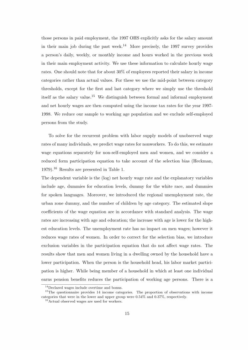
those persons in paid employment, the 1997 OHS explicitly asks for the salary amount
in their main job during the past week.14 More precisely, the 1997 survey provides
a person’s daily, weekly, or monthly income and hours worked in the previous week
in their main employment activity. We use these information to calculate hourly wage
rates. One should note that for about 30% of employees reported their salary in income
categories rather than actual values. For these we use the mid-point between category
thresholds, except for the first and last category where we simply use the threshold
itself as the salary value.15 We distinguish between formal and informal employment
and net hourly wages are then computed using the income tax rates for the year 1997-
1998. We reduce our sample to working age population and we exclude self-employed
persons from the study.
To solve for the recurrent problem with labor supply models of unobserved wage
rates of many individuals, we predict wage rates for nonworkers. To do this, we estimate
wage equations separately for non-self-employed men and women, and we consider a
reduced form participation equation to take account of the selection bias (Heckman,
1979).16 Results are presented in Table 1.
The dependent variable is the (log) net hourly wage rate and the explanatory variables
include age, dummies for education levels, dummy for the white race, and dummies
for spoken languages. Moreover, we introduced the regional unemployment rate, the
urban zone dummy, and the number of children by age category. The estimated slope
coefficients of the wage equation are in accordance with standard analysis. The wage
rates are increasing with age and education; the increase with age is lower for the high-
est education levels. The unemployment rate has no impact on men wages; however it
reduces wage rates of women. In order to correct for the selection bias, we introduce
exclusion variables in the participation equation that do not affect wage rates. The
results show that men and women living in a dwelling owned by the household have a
lower participation. When the person is the household head, his labor market partici-
pation is higher. While being member of a household in which at least one individual
earns pension benefits reduces the participation of working age persons. There is a14Declared wages include overtime and bonus.15The questionnaire provides 14 income categories. The proportion of observations with income
categories that were in the lower and upper group were 0.54% and 0.37%, respectively.16Actual observed wages are used for workers.
15
significant positive parameter of the Inverse of the Mill’s Ratio (IMR) for both men
and women.
The empirical application of this paper relies upon the theoretical framework that
considers three family types. In terms of defining family types, we divide individuals
in four different age groups: “under 18”, “18-40”, “41-64”, and “64 and more”. In Table
A.5 in the Appendix, we provide age group repartition for the total population and
a distinct repartition according to marital status. Then we defined couples. Three
types of couples exist: young couple, middle-age couple and old couple, corresponding
respectively to the second, third and fourth age group.17 First, we define nuclear
couple household a man and woman who are married or living together as a couple.
Observations of households where more than one couple lives are excluded. Second,
we define single-nuclear family every single, widow or divorced adult living alone. We
dropped all observations of households where an old single person lives and/or where an
old couple lives. Thus, the extended household structure is one adult and one couple
who cohabitate. This classification does not exclude the case where these families
might have children. With respect to the theoretical model developed, we restricted
the empirical analysis to these family structures, and hence dropped all households
where other possible extended household structures might appear.18 We exclude from
the analysis households where at least one individual aged “18-24” lives, and we define
children those who are less than 18.
After controlling for missing values, we are left with a total number of 8,212 ob-
servations among which 5,605 observations are for couple families, 2,111 are for single
adult families and the rest is for extended families. In 42.5% of extended families,
only one member has a paid job and in 31% of the cases two members are employed.
For 3,075 couple families, only one of the two partners is employed and in 90% of the
observations it is the husband. In 29% of couple families in our sample both wife and
husband work. For single families, up to 65% of men are working and nearly 48% of
women have a job. In Table 2, we report some statistics of the labor market for the dif-17Note that the couple type is defined relatively to the husband age. However, we kept observations
with both partners from working age population.18For instance, we do not consider 1,009 households where a single adult or/and a couple lives with
an old person. However, in the South African context, the amount of pensions might have an importantimpact especially that the South African social pension is so generous (Duflo, 2003).
16

ferent household structures we composed. We can see that labor market participation
is lower in extended families. More specifically, employment dummy falls from 0.650 to
0.375 for single men and from 0.478 to 0.299 for single women. Similarly, it decreases
from 0.780 to 0.673 for married men and from 0.340 to 0.274 for married women. In our
study sample, weekly working hours are 48.2 for married men, 42.6 for married women,
48.6 for single men and 44.6 for single women. In Figure 1 we plot the distribution of
the working hours per week from the sample of employed men and women.
As the labor choice in our study is discrete, every person in nuclear or extended
households chooses whether to participate in the labor market on a full time basis or to
stay out of it. In the empirical part of our study, we fix the week time endowment at 80
hours, and if the person decides to join the labor market the number of working hours
per week is 45.19 The net hourly wage rates that are used result from the previous two-
stage estimation. The non-labor income includes disability grant, state maintenance
grant, private maintenance by father/former spouse (not living in the same household at
the moment of the survey), care dependency grant, foster care grant, and any financial
support.
5 The Empirical Specification and the Estimation
5.1 The likelihood function
In the data, the unit of observation is the household. Thus, every household constituted
of a single adult or a couple, either living alone or cohabitating within an extended
family, is considered one observation. The observations are indexed by i or j. A
household where a single adult and a couple live together (for instance, if the ith family
cohabitates with the jth family) constitutes an extended household.
For the reasons which were previously exposed, the self-selection of families between
these types of demographic structures is certainly not exogenous to labor supply deci-
sions. To model the latter we have thus to formulate a selection equation. For extended
families, we observe a large range of variables characterizing both families that may af-19The regulation of working hours in South Africa states that ordinary hours of work, i.e., excluding
overtime, may not be more than 45 hours per week. Any additional hour has to be considered overtimefor which a specified amount of additional remuneration is prescribed. Note that overtime is limitedto 10 hours per week and may not exceed 3 hours per day. Furthermore, our total data sample showsthat, in average, both men and women work 45 hours per week.
17

fect the decision to cohabitate (including both families’ income).20 For nuclear families,
we have limited information about the single(s) or the couple(s) with which this family
could match. To exploit the maximum of variables in the specification of the selection,
the idea is then to use two selection equations, one for each type of nuclear family. To
do so, for each family i of structure r in the data set, we define a dummy variable pri
which is equal to one if the family i does not cohabitate with another family and equal
to zero otherwise. The selection equation can then be written as:
pr∗i = αrxi − εp,ri ,
where pr∗i is a latent variable, such that
pri = 1
pri = 0
if
if
pr∗i > 0,
pr∗i ≤ 0,
and εp,ri is a stochastic term that is normally distributed with zero mean and unit
variance. If the ith family and the jth family live together, then pr∗i ≤ 0 and ps∗j ≤ 0.
To construct the likelihood function, we then distinguish two regimes depending on the
type of the household.
A. The Contribution of Nuclear Families. To compute the contribution to the
likelihood function of the observation of a family i of structure r living alone, the
random terms that represent taste heterogeneity has to be decomposed as follows:
νri = ωri εν,ri + σrεp,ri (5)
where εν,ri and εp,ri are normally distributed stochastic terms with zero mean and unit
variance. The decision to participate in the labor market will be endogenous to the
decision to cohabitate if σr 6= 0.
Following the discussion that precedes, let us note that the family i will live alone if and
only if εp,ri < αrxi. The probability that the family i lives alone and actually chooses
20Nevertheless, the characteristics of all the families that were potentially candidates for the consti-tution of the extended family are not observed.
18

alternative k∗ is then given by
Pr(k = k∗) = Φ(αrxi)×∫ αrxi
−∞Fk∗(ε
p,ri ) · φ(εp,ri ) · dεp,ri (6)
where
Fk∗(εp,ri ) =
∫ +∞
−∞
exp (urik∗)∑2r
k=1 exp(urik) · φν|ε (νri | ε
p,ri ) · dνri
is the conditional probability of choosing alternative k∗ when εp,ri is given, φ and Φ(·)
designate respectively the density function and the cumulative function of the (univari-
ate or multivariate) standardized normal distribution, and φν|ε the density function of
the conditional distribution of νri given εp,ri . The first term on the left-hand-side of
expression (6) is the marginal probability of not cohabitating; the second term is the
conditional probability of selecting alternative k∗ provided that the family does not
cohabitate with another family.
B. The Contribution of Extended Families. The introduction of taste hetero-
geneity is much easier if the random terms of the two families are not correlated. Hence
we shall adopt this assumption here. The family i of structure r and the family j of
structure s will live together if and only if εp,ri > αrxi and εp,sj > αsxj . In the extended
family, the joint probability that the family i selects alternative k∗ and that the family
j selects alternative l∗ is given by
Pr(k = k∗, l = l∗) = [1− Φ(αrxi)]× [1− Φ(αsxj)]
×∫ +∞
αrxi
Fk∗(εp,ri ) · φ(εp,ri ) · dεp,ri
×∫ +∞
αsxj
Fl∗(εp,sj ) · φ(εp,sj ) dεp,sj
where Fk∗(εp,ri ) and Fl∗(ε
p,sj ) are defined as above. The contribution to the likelihood
is thus simply the product of the conditional probability of choosing alternative k∗ and
that of choosing alternative l∗, given that both families cohabitate.
19
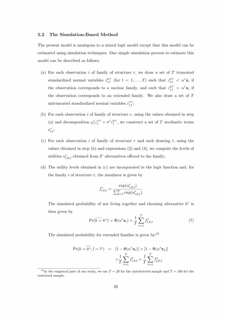
5.2 The Simulation-Based Method
The present model is analogous to a mixed logit model except that this model can be
estimated using simulation techniques. One simple simulation process to estimate this
model can be described as follows.
(a) For each observation i of family of structure r, we draw a set of T truncated
standardized normal variables εp,ri,t (for t = 1, . . . , T ) such that εp,ri,t < αrxi if
the observation corresponds to a nuclear family, and such that εp,ri,t > αrxi if
the observation corresponds to an extended family. We also draw a set of T
untruncated standardized normal variables εν,ri,t ;
(b) For each observation i of family of structure r, using the values obtained in step
(a) and decomposition ωri εν,ri + σrεp,ri , we construct a set of T stochastic terms
νri,t;
(c) For each observation i of family of structure r and each drawing t, using the
values obtained in step (b) and expressions (2) and (3), we compute the levels of
utilities uri,k,t obtained from 2r alternatives offered to the family;
(d) The utility levels obtained in (c) are incorporated in the logit function and, for
the family i of structure r, the simulator is given by
f ri,k,t =exp(uri,k,t)∑2r
k=1 exp(uri,k,t)
The simulated probability of not living together and choosing alternative k∗ is
then given by ˜Pr(k = k∗) = Φ(αrxi)×1T
T∑t=1
f ri,k,t (7)
The simulated probability for extended families is given by:21
˜Pr(k = k∗, l = l∗) = [1− Φ(αrxi)]× [1− Φ(αsxj)]
× 1T
T∑t=1
f ri,k,t ×1T
T∑t=1
fsj,k,t
21In the empirical part of our study, we use T = 20 for the unrestricted sample and T = 100 for therestricted sample.
20
5.3 Empirical Results
Our theoretical model is estimated separately on the 8,212-observation sample as well
as on the reduced sample of no-children households - as the model might be not well
adapted to treat of children presence within the household. The remaining 2,571 ob-
servations that do not enter Table A.6 constitute the restricted sample of households
without children.22
5.3.1 A. Participation to Nuclear vs. Extended Families
Table 3 shows the estimation results of the participation to nuclear families for singles
and couples, respectively. The parameter estimates of the unrestricted sample are
qualitatively similar to those of the restricted sample. The coefficients xs01 and xc01
of the dummy variables of the age category “18-40” are significant for single adults
and for couples, and show that younger single adults are more likely to be members
of extended families while couples with men aged “18-40” are more likely to be in
nuclear families compared to those where men are aged “41-64”. Moreover, it seems
that single White adults are more likely to be in nuclear families than their Black,
Asian and Colored counterparts. This might be due to privacy desire and/or to worker
migration. Similarly, a big proportion of extended couple families are from the non-
White population.
Importantly, we observe in both the restricted and unrestricted samples that higher
wages affect negatively the single adult’s participation decision to extended family,
while wages of married men and women seem not to affect the couple’s cohabitation
decision. In our sample, single adult females are more likely to be in nuclear families
than single adult males. The estimated parameters of the urban dummy - significant in
the unrestricted sample only - are negative meaning that living in urban areas increases
the probability of cohabitation of an adult and a couple. This result contrasts with
the common thought according to which nuclear family structures are predominant
in urban areas whereas extended family structures are more prevalent in rural areas
(Burch, 1967). This negative urban parameter estimate might be due to the fact that we
consider a specific structure of extended family in our empirical study. In contrast to the22Among these observations, 1,196 are for single-nuclear families, 1,267 for couple-nuclear families,
and 108 for extended families.
21

traditional view, one might think that there exists a difference in family arrangements
among Whites and Blacks. More precisely, for some reasons of cultural preferences
and affordability, White South Africans succeed to maintain the nuclear family system,
while non-White South Africans remain in extended families independently from the
living area.
The empirical research of the consequences of living in an extended family on indi-
vidual’s labor supply is crucial given the endogeneity of belonging to extended family
in labor supply decision (interdependency of choices). Thus our empirical study relies
on the availability of instruments that explain the decision of a single adult or a couple
to cohabitate but do not explain labor supply. The 1997 OHS data provide information
on parents and family members of questioned persons like whether mother, father or
sister aged more than 15 are still alive and whether there exists an adult family member
who does not live in the household. By introducing these variables in the participation
equation to nuclear family, we find that having his/her own mother still alive affects
negatively the single adult’s participation to extended family. However, this effect dif-
fers among people belonging to the“18-40”age group and those belonging to the“41-64”
age group. In particular, if we look at the estimated parameters xs09 and xs13 we con-
clude that single adults aged more than 40 are more likely to be in nuclear families
when the mother is still alive. Similarly, the negative sign of xs14 shows that older
adults are more likely to live alone even if their fathers are still alive. These effects are
significant solely in the unrestricted sample. Furthermore, we notice that single adults
- with or without children - who live in extended families are more likely to have a
family member who does not live in the same household. The reason for that could be
the necessity in extended families for at least one member to leave in order to work and
help supporting the family or to get more privacy. However, extended family members
are less likely to have a sister aged more than 15 still alive. This result is consistent
with the unrestricted sample as well as the restricted sample. Concerning couples, we
observe that living in an extended family is negatively affected when the wife is aged
less than or equal to 40 and her mother is alive. The presence of a family member
who is not living in the household at the moment of the survey affects positively the
couple’s decision to cohabitate.
22

5.3.2 B. Labor Supply Estimation Results
We start by reporting, from Table 4, the estimates of the parameters of single adults’
labor supply, separately for men and women. For these estimations we take “not work-
ing” as the base category, and therefore all the parameters are interpreted as changes
in probability of working relative to not working. The slope parameters of the utility
functions relative to the decisions of not working - β0sm and β0sf - and working - β1sm
and β1sf - are positive and significant for single men and women. Given that β1sm and
β1sf are positive, an increase in the wage rate implies a substitution of leisure to work
for men and women, as the price of leisure increases, and the individual probability
to work increases. Non-participation probability is increasing with non-labor income,
since β0sm and β0sf are greater than β1sm and β1sf , respectively. Thus, leisure is a
normal good. A similar analysis is valid for couples concerning their decisions not to
work or not. In fact, the estimations give the labor supply of couples when the base
category corresponds to the case where both husband and wife do not work. Three
other alternative categories remain. Table 4 shows the estimated slope parameters of
all possible alternatives: β00c, β01c, β10c and β11c. The results confirm the fact that
leisure is a normal good as β.. is smaller when the number of working hours is higher.
Essentially, this is verified for the β..s’ estimations except for the β11c that is slightly
larger than β10c; yet this difference is not significant.
The decision to participate in the labor market is endogenous to the decision to
cohabitate. There is a non-observed heterogeneity that affects the decision to partic-
ipate to nuclear family εp,ri that also affects labor decision. Although not significant,
the positive sign of the parameters of the truncated standard normal, σs and σc, that
enter the taste heterogeneity expression shows that being member of an extended fam-
ily decreases the labor market participation of the single adults and/or the couples.
Furthermore, there is a non-observed heterogeneity captured by the individual random
effects. The estimated parameters ωs and ωc represent the marginal utility on con-
sumption for singles and couples. These results are similar for the unrestricted and
restricted samples.
In Table 5 and Table 6, we present the estimates of the parameters of the intercept
of the utility function for single adults - men and women separately - and for cou-
23

ples, respectively. In both the restricted and unrestricted samples, the White single’s
probability to participate in the labor market is lower with respect to the other race
groups for both men and women. Young single men and women are more likely to work
than those aged more than 40. Moreover, living in an urban area affects negatively the
participation decision of single men and positively that of single women. The param-
eter estimates of the unrestricted sample show that while single men labor supply is
not affected by the presence of young children, single women reduce their labor supply
in the presence of children; this reduction is higher when children are younger. The
corresponding results for couples are as follows. The labor supply of Whites decreases
when at least one of the two partners is working relative to the other race categories.
Here again, the participation of women in the labor market is negatively affected by
the presence of young children (see Alternatives 2 and 4). However, the participation
decision of married men when their wives are not working is positively affected by the
existence within the household of children aged “0-3”. Furthermore, the couples where
the husband is aged “18-40” are more likely to have at least one of both partners work-
ing compared to couples where the husband is older than 40. Finally, the probability of
observing a couple where the wife is employed while the husband is not increases when
the couple lives in urban areas.
5.3.3 C. Sharing Rule Parameters
The estimation results show that, at the mean sample, the single’s share of non-labor
income constitutes 25.15% of total non labor income in the unrestricted sample and
11.26% in the restricted sample. The distributions of single’s share are represented in
Figure 2 for both the restricted and unrestricted samples.
In Table 7 we present the results of the estimated parameters of the sharing rule in
families where a single adult and a couple cohabitate. These parameters represent the
impact of a marginal change in one of the variables on the non-labor income accruing to
the single adult when he/she is part of an extended family. According to our estimates,
a R 1 increase in the non-labor income induces an increase in adult’s share of 0.065.
Moreover, an increase in the single adult’s hourly wage rate reduces his/her share from
non-labor income. At the mean of hours worked by singles, an increase of R 2,480
reduces single’s share of non-labor income of R 273. The husband’s labor income has
24
no effect on the adult’s share. However, an increase in wife’s labor income induces a
significant increase in adult’s share of total non-labor income. More precisely, a R 1
increase of labor income (that is equivalent to an annual increase of R 2,178 in her labor
income at the mean of hours worked by women in the extended family) translates into
an increase in the amount of non-labor income accruing to the single adult of R 2,802.
The estimated parameter of male dummy is 0.027 and 0.052 in the unrestricted and
restricted samples, respectively. It supports the idea that single men who cohabitate
with couples get a higher share of non-labor income than do single women. Although not
significant, the presence of children in the household reduces single’s share of non-labor
income. Living in urban areas relative to rural areas has no effect on the intrahousehold
allocation of non-labor income. However, we notice a difference among race categories
so that single White adults have a smaller share than singles of other races. We also
find that belonging to the age category “18-40” has a small positive effect on non-labor
income accruing to singles in extended families.
Concerning the economies scale in consumption resulting from cohabitation, the
estimates are given in Table 8. As presented in the theoretical model, we introduced
different parameters for the singles and the couples. For the singles, we also distinguish
between men and women. Thus, we estimate κc, κm and κf in the unrestricted and
restricted samples for couples, single males and single females, respectively. We find
that κm and κf are lower than unity, a proof that there exists a significant gain for
adults from cohabitating. These economies of scale are about 75% for single men and
67% for single women in the unrestricted sample. Concerning couples who decided to
cohabitate and to share their resources, we find that there are no economies of scale; yet
the result remains valid as the gains from cohabitation are already exploited when living
in couple. Unexpectedly, in the restricted sample, the parameters of scale economies
are 0.345 and 0.244, respectively for single men and single women. One might explain
this result by supposing that, in extended families without children, a single accepts a
low share from the intrahousehold allocation provided that he/she benefits from high
economies of scale in consumption.23
23Nevertheless, we note that κm and κf in the restricted sample remains low though.
25
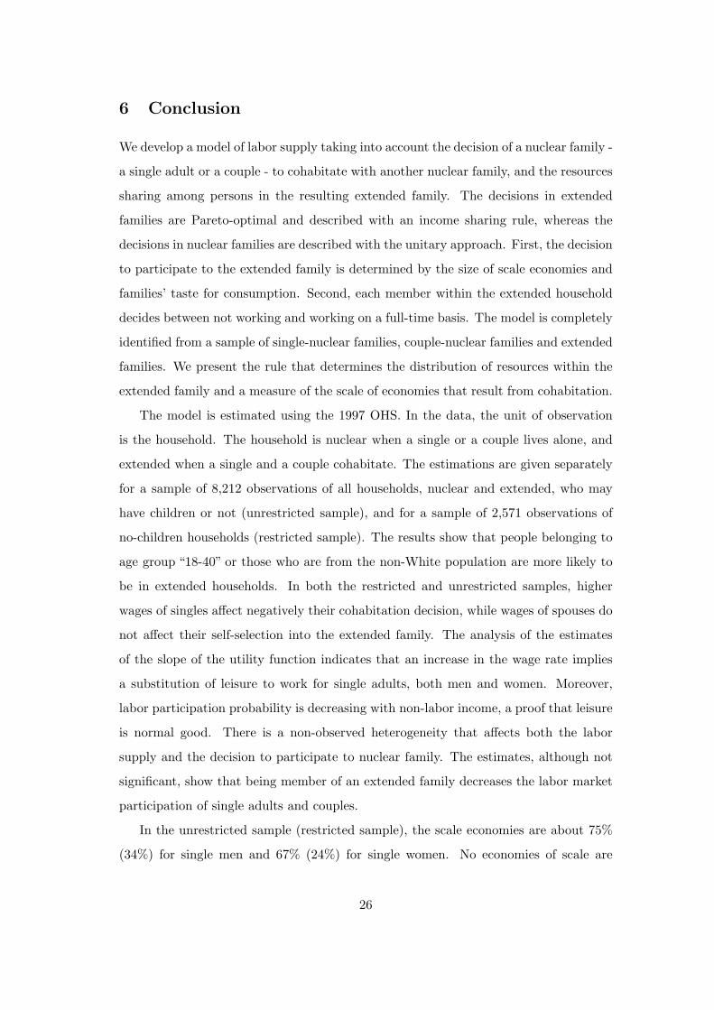
6 Conclusion
We develop a model of labor supply taking into account the decision of a nuclear family -
a single adult or a couple - to cohabitate with another nuclear family, and the resources
sharing among persons in the resulting extended family. The decisions in extended
families are Pareto-optimal and described with an income sharing rule, whereas the
decisions in nuclear families are described with the unitary approach. First, the decision
to participate to the extended family is determined by the size of scale economies and
families’ taste for consumption. Second, each member within the extended household
decides between not working and working on a full-time basis. The model is completely
identified from a sample of single-nuclear families, couple-nuclear families and extended
families. We present the rule that determines the distribution of resources within the
extended family and a measure of the scale of economies that result from cohabitation.
The model is estimated using the 1997 OHS. In the data, the unit of observation
is the household. The household is nuclear when a single or a couple lives alone, and
extended when a single and a couple cohabitate. The estimations are given separately
for a sample of 8,212 observations of all households, nuclear and extended, who may
have children or not (unrestricted sample), and for a sample of 2,571 observations of
no-children households (restricted sample). The results show that people belonging to
age group “18-40” or those who are from the non-White population are more likely to
be in extended households. In both the restricted and unrestricted samples, higher
wages of singles affect negatively their cohabitation decision, while wages of spouses do
not affect their self-selection into the extended family. The analysis of the estimates
of the slope of the utility function indicates that an increase in the wage rate implies
a substitution of leisure to work for single adults, both men and women. Moreover,
labor participation probability is decreasing with non-labor income, a proof that leisure
is normal good. There is a non-observed heterogeneity that affects both the labor
supply and the decision to participate to nuclear family. The estimates, although not
significant, show that being member of an extended family decreases the labor market
participation of single adults and couples.
In the unrestricted sample (restricted sample), the scale economies are about 75%
(34%) for single men and 67% (24%) for single women. No economies of scale are
26
observed for couples. The parameters of the sharing rule show that the share devoted
to the single adult is positively related to the household non-labor income. Furthermore,
the adult’s share in non-labor income decreases in his/her wage rate but increases in
both husband and wife wages. The estimated parameter of male dummy shows that
single males have a higher share than single female adults.
References
[1] Angel, R. and M. Tienda. 1982. “Determinants of Extended Household Structure:Cultural Pattern or Economic Need?” American Journal of Sociology 87, 1360-1383.
[2] Bargain, O. 2005. “On Modeling Household Labor Supply with Taxation”. IZADiscussion Papers, No. 1455.
[3] Barten, A. 1964. “Family Composition, Prices, and Expenditure Patterns”, in Hart,P.E., G. Mills and J.K. Whitaker (eds.), Econometric Analysis for National Eco-nomic Planning, London, Butterworths.
[4] Behrman, J. and B. Wolfe. 1984. “Labor Force Participation and Earnings Deter-minants for Women in the Special Conditions of Developing Countries”. Journal ofDevelopment Economics 15, 259-288.
[5] Bertrand, M., S. Mullainathan and D. Miller. 2003. “Public Policy and ExtendedFamilies: Evidence from Pensions in South Africa”. World Bank Economic Review17, 27-50.
[6] Blundell, R., P-A. Chiappori, T. Magnac and C. Meghir. 2007. “Collective LabourSupply: Heterogeneity and Nonparticipation”. Review of Economic Studies 74, 417-445.
[7] Brock W.A. and S. Durlauf. 2001. “Interaction-Based Models”, in Heckman J.J.and E. Leamer (eds), Handbook of Econometrics, Vol. 5, Chap. 54, pp. 3297-3380,Amsterdam: Elsevier.
[8] Browning, M., P-A. Chiappori and A. Lewbel. 2008. “Estimating ConsumptionEconomies of Scale, Adult Equivalence Scales, and Household Bargaining Power”.Boston College Working Papers in Economics, No. 588, revised 2008.
[9] Burch, T.K. 1967. “The Size and Structure of Families: A Comparative Analysis ofCensus Data”. American Journal of Sociology 32, 347-363.
27

[10] Case, A. and A. Deaton. 1998. “Large Cash Transfers to the Elderly in SouthAfrica”. Economic Journal 108, 1330-1361.
[11] Chiappori, P-A. 1988. “Rational Household Labor Supply”. Econometrica 56, 63-89.
[12] Chiappori, P-A. 1992. “Collective Labor Supply and Welfare”. Journal of PoliticalEconomy 100, 437-467.
[13] Chiappori, P-A. and I. Ekeland. 2006. “The Micro Economics of Group Behavior:General Characterization”. Journal of Economic Theory 130, 1-26.
[14] Chiappori, P-A. and I. Ekeland. 2009. “The Microeconomics of Efficient GroupBehavior: Identification”. Econometrica 77, 763-799.
[15] Couprie, H. 2007. “Time Allocation within the Family: Welfare Implications ofLife in a Couple”. Economic Journal 117, 287-305.
[16] Deaton, A. and C. Paxson. 1998. “Economies of Scale, Household Size and theDemand for Food”. Journal of Political Economy 106, 897-930.
[17] Duflo, E. 2003. “Grandmothers and Granddaughters: Old-Age Pensions and In-trahousehold Allocation in South Africa”. World Bank Economic Review 17, 1-25.
[18] Duflo, E. 2003. “Child Health and Household Resources in South Africa: Evidencefrom the Old Age Pension Program”. American Economic Review 90, 393-398.
[19] Fafchamps, M. and A. Quisumbing. 2003. “Social Roles, Human Capital, and theIntrahousehold Division of Labor: Evidence from Pakistan”. Oxford Economic Pa-pers 38, 47-82.
[20] Foster, A. and M. Rosenzweig. 2002. “Household Division, and Rural EconomicGrowth”. Review of Economic Studies 69, 839-869.
[21] Gong, X. and A. van Soest. 2002. “Family Structure and Female Labor Supply inMexico City”. Journal of Human Resources 37, 163-191.
[22] Gronau, R. 1991. “The Intrafamily Allocation of Goods - How to Separate theAdult from the Child”. Journal of Labor Economics 9, 207-235.
[23] Heckman, J. 1979. “Sample Selection Bias as a Specification Error”. Econometrica47, 153-61.
28

[24] Heckman, J. 1990. “Varieties of Selection Bias”. American Economic Review 80,331-338.
[25] Kochar, A. 2000.“Parental Benefits from Intergenerational Coresidence: EmpiricalEvidence from Rural Pakistan”. Journal of Political Economy 108, 1184-1209.
[26] Lanjouw, P. and M. Ravallion. 1995. “Poverty and Household Size”. EconomicJournal 105, 1415-1434.
[27] Lewbel, A. and K. Pendakur. 2009. “Tricks with Hicks: The EASI Demand Sys-tem”. American Economic Review 99, 827-863.
[28] Newman, J.L. and P.J. Gertler. 1994. “Family Productivity, Labor Supply, andWelfare in a Low Income Country”. Journal of Human Resources 29, 989-1026.
[29] Pirouz, F. 2005. “Have Labour Market Outcomes Affected Household Structure inSouth Africa? A Descriptive Analysis of Households”. University of the Witwater-srand WP 05/100.
[30] Quisumbing, A. and J. Maluccio. 2003. “Resources at Marriage and IntrahouseholdAllocation: Evidence from Bangladesh, Ethiopia, Indonesia, and South Africa”.Oxford Bulletin of Economics and Statistics 65, 283-328.
[31] Thirumurthy, H., J.G. Zivin, and M. Goldstein. 2008. “The Economic Impact ofAIDS Treatment: Labor Supply in Western Kenya”. Journal of Human Resources43, 511-552.
[32] Van Soest, A. 1995.“Structural Models of Family Labor Supply: A Discrete ChoiceApproach”. Journal of Human Resources 30, 63-88.
[33] Wittenberg, M. and M. Collinson. 2005. “Restructuring Households in Rural SouthAfrica: Reflections on Average Household Size in the Agincourt Sub-District 1992-2003”. School of Economics, University of Cape Town and University of the Witwa-tersrand.
29

Table 1: Estimation ResultsParticipation Model and Wage Regression
Participation Equation Wage Equation
Males Females Males Females
Age 0.249∗∗∗ 0.219∗∗∗ 0.107∗∗∗ 0.071∗∗∗
Age2 -0.003∗∗∗ -0.003∗∗∗ -0.001∗∗∗ -0.001∗∗∗
White 0.039 -0.106∗∗∗ 0.499∗∗∗ 0.358∗∗∗
Black 0.080 -0.012 0.067 -0.052English 0.341∗∗∗ 0.294∗∗∗ 0.385∗∗∗ 0.305∗∗∗
Afrikaans 0.156∗∗ 0.270∗∗∗ 0.109∗∗ 0.052Married 0.349∗∗∗ -0.213∗∗∗ 0.246∗∗∗ 0.056∗∗∗
Educ1 0.384∗∗ 0.494∗∗∗ -0.079 0.116Educ2 0.460∗∗∗ 0.140 0.391∗∗∗ 0.100Educ3 0.078 -0.265∗∗ 0.644∗∗∗ 0.501∗∗∗
Educ4 0.345∗∗∗ -0.111 1.196∗∗∗ 1.134∗∗∗
Educ1*Age -0.012∗∗∗ -0.010∗∗ 0.005 -0.002Educ2*Age -0.011∗∗∗ -0.003 -0.002 0.005Educ3*Age -0.002 0.009∗∗∗ -0.003 0.002Educ4*Age -0.003 0.016∗∗∗ -0.006∗∗∗ 0.007∗∗
Urban zone 0.037∗ 0.217∗∗∗ 0.469∗∗∗ 0.419∗∗∗
Unemployment Rate -0.040∗∗∗ -0.019∗∗∗ 0.002 -0.005∗∗
Household Head 0.717∗∗∗ 0.224∗∗∗
Own House -0.545∗∗∗ -0.337∗∗∗
Child0 3n 0.054∗∗∗ -0.034∗∗∗
Child4 6n -0.009 -0.035∗∗∗
Child7 12n -0.055∗∗∗ -0.051∗∗∗
Pension dummy -0.203∗∗∗ -0.152∗∗∗
Inverse Mills Ratio 0.168∗∗∗ 0.153∗∗∗
Constant -3.869∗∗∗ -4.070∗∗∗ -1.796∗∗∗ -1.202∗∗∗
Obs. 34,013 41,337 13,061 9,320
(1) Significance levels of 10%, 5% and 1% are noted ∗, ∗∗ and ∗∗∗, respectively;(2) English and Afrikaans are dummies for spoken languages;(3) The unemployment rate is represented by region (for the 9 provinces in South
Africa), separately for men and women;(4) Pension dummy=1 if there is at least one individual in the household who has
a pension;(5) Child0 3n, Child4 6n, and Child7 12n are the number of children aged 0-3, 4-6,
and 7-12 years, respectively;(6) Household head is a dummy for whether the person is the head of the household
and Own house is the dummy for whether household’s members are owner oftheir house;
(7) There are 4 dummies for the education levels that go from the junior primary(Educ1 ) to the university (Educ4 ). No education is the reference category.
30
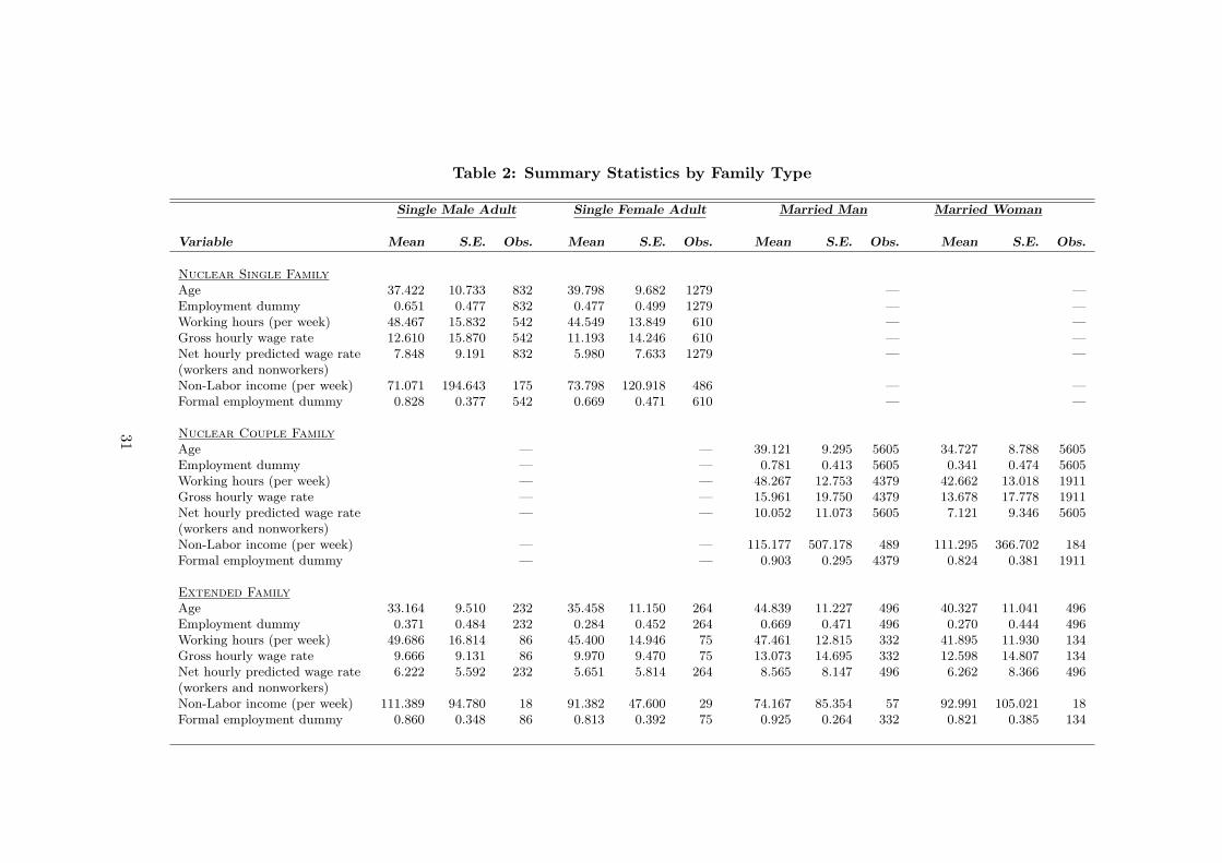
Table 2: Summary Statistics by Family Type
Single Male Adult Single Female Adult Married Man Married Woman
Variable Mean S.E. Obs. Mean S.E. Obs. Mean S.E. Obs. Mean S.E. Obs.
Nuclear Single FamilyAge 37.422 10.733 832 39.798 9.682 1279 — —Employment dummy 0.651 0.477 832 0.477 0.499 1279 — —Working hours (per week) 48.467 15.832 542 44.549 13.849 610 — —Gross hourly wage rate 12.610 15.870 542 11.193 14.246 610 — —Net hourly predicted wage rate 7.848 9.191 832 5.980 7.633 1279 — —(workers and nonworkers)Non-Labor income (per week) 71.071 194.643 175 73.798 120.918 486 — —Formal employment dummy 0.828 0.377 542 0.669 0.471 610 — —
Nuclear Couple FamilyAge — — 39.121 9.295 5605 34.727 8.788 5605Employment dummy — — 0.781 0.413 5605 0.341 0.474 5605Working hours (per week) — — 48.267 12.753 4379 42.662 13.018 1911Gross hourly wage rate — — 15.961 19.750 4379 13.678 17.778 1911Net hourly predicted wage rate — — 10.052 11.073 5605 7.121 9.346 5605(workers and nonworkers)Non-Labor income (per week) — — 115.177 507.178 489 111.295 366.702 184Formal employment dummy — — 0.903 0.295 4379 0.824 0.381 1911
Extended FamilyAge 33.164 9.510 232 35.458 11.150 264 44.839 11.227 496 40.327 11.041 496Employment dummy 0.371 0.484 232 0.284 0.452 264 0.669 0.471 496 0.270 0.444 496Working hours (per week) 49.686 16.814 86 45.400 14.946 75 47.461 12.815 332 41.895 11.930 134Gross hourly wage rate 9.666 9.131 86 9.970 9.470 75 13.073 14.695 332 12.598 14.807 134Net hourly predicted wage rate 6.222 5.592 232 5.651 5.814 264 8.565 8.147 496 6.262 8.366 496(workers and nonworkers)Non-Labor income (per week) 111.389 94.780 18 91.382 47.600 29 74.167 85.354 57 92.991 105.021 18Formal employment dummy 0.860 0.348 86 0.813 0.392 75 0.925 0.264 332 0.821 0.385 134
31

Table 3: Estimation Results of Participation to Nuclear Families
Unrestricted Sample Restricted Sample———————————– ———————————
Parameter Variable Estimates Estimates
Single Adults
xs00 constant 2.385 (0.362) 2.980 (0.642)xs01 age ad -0.250 (0.107) -0.599 (0.246)xs02 adult’s (log) hourly wage 0.190 (0.042) 0.167 (0.078)xs03 white ad 0.525 (0.144) 0.242 (0.230)xs04 black ad 0.211 (0.212) 0.425 (0.359)xs05 english ad -0.704 (0.230) -0.731 (0.376)xs06 afrikaans ad -0.481 (0.211) -0.291 (0.368)xs07 urban dummy -0.244 (0.071) -0.175 (0.140)xs08 male ad dummy -0.355 (0.066) -0.250 (0.139)xs09 mother ad 0.307 (0.134) 0.096 (0.283)xs10 father ad -0.090 (0.175) -0.277 (0.354)xs11 sister15 ad 0.359 (0.071) 0.547 (0.125)xs12 adult nohh ad -0.676 (0.078) -1.098 (0.155)xs13 mother ad * age ad -0.342 (0.162) -0.231 (0.343)xs14 father ad * age ad -0.341 (0.192) -0.240 (0.386)
Couples
xc00 constant 0.847 (0.313) 0.255 (0.692)xc01 age m 0.259 (0.087) 0.499 (0.231)xc02 husband’s (log) hourly wage -0.058 (0.037) 0.008 (0.081)xc03 wife’s (log) hourly wage 0.039 (0.041) -0.059 (0.090)xc04 white m 0.612 (0.102) 0.565 (0.187)xc05 black m 0.139 (0.166) 0.450 (0.351)xc06 english m -0.035 (0.181) 0.111 (0.371)xc07 afrikaans m 0.050 (0.164) 0.258 (0.354)xc08 urban dummy -0.109 (0.062) -0.006 (0.139)xc09 mother m 0.138 (0.073) -0.081 (0.134)xc10 father m 0.300 (0.106) 0.470 (0.233)xc11 mother f -0.027 (0.081) -0.042 (0.147)xc12 father f 0.078 (0.108) 0.073 (0.194)xc13 sister15 m 0.070 (0.064) 0.145 (0.127)xc14 sister15 f -0.008 (0.064) 0.061 (0.124)xc15 adult nohh -0.264 (0.063) 0.019 (0.121)xc16 mother m * age m -0.068 (0.106) 0.078 (0.259)xc17 father m * age m -0.164 (0.128) -0.343 (0.298)xc18 mother f * age f 0.171 (0.093) 0.068 (0.203)xc19 father f * age f 0.090 (0.123) -0.089 (0.249)
(1) Extensions ” m”, ” f ” and ” ad” denote characteristics relative to married man, marriedwoman and single adult, respectively;
(2) Standard errors are in parentheses.
32
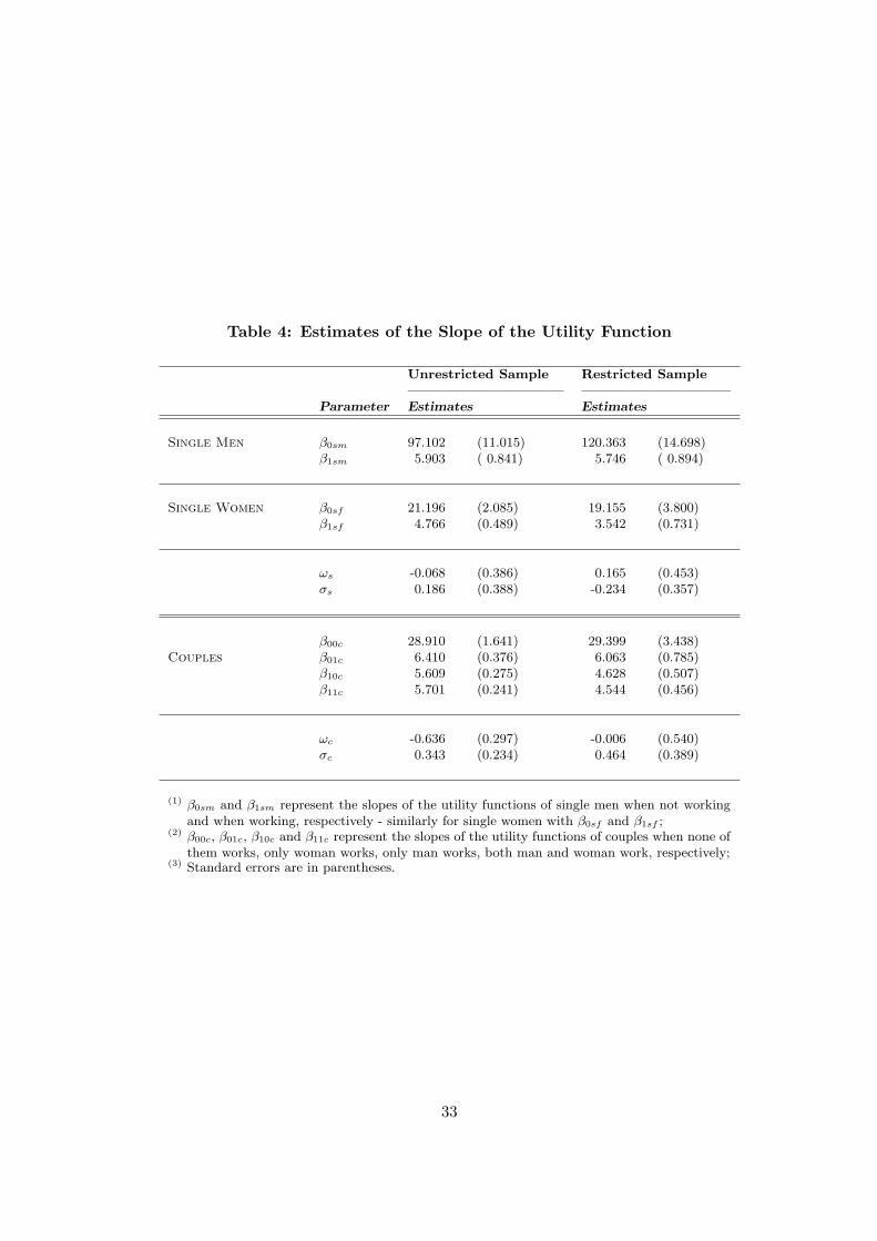
Table 4: Estimates of the Slope of the Utility Function
Unrestricted Sample Restricted Sample———————————– ———————————
Parameter Estimates Estimates
Single Men β0sm 97.102 (11.015) 120.363 (14.698)β1sm 5.903 ( 0.841) 5.746 ( 0.894)
Single Women β0sf 21.196 (2.085) 19.155 (3.800)β1sf 4.766 (0.489) 3.542 (0.731)
ωs -0.068 (0.386) 0.165 (0.453)σs 0.186 (0.388) -0.234 (0.357)
β00c 28.910 (1.641) 29.399 (3.438)Couples β01c 6.410 (0.376) 6.063 (0.785)
β10c 5.609 (0.275) 4.628 (0.507)β11c 5.701 (0.241) 4.544 (0.456)
ωc -0.636 (0.297) -0.006 (0.540)σc 0.343 (0.234) 0.464 (0.389)
(1) β0sm and β1sm represent the slopes of the utility functions of single men when not workingand when working, respectively - similarly for single women with β0sf and β1sf ;
(2) β00c, β01c, β10c and β11c represent the slopes of the utility functions of couples when none ofthem works, only woman works, only man works, both man and woman work, respectively;
(3) Standard errors are in parentheses.
33
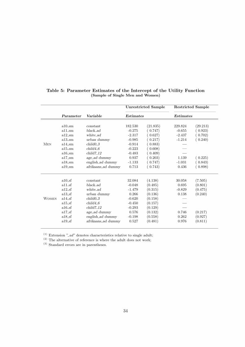
Table 5: Parameter Estimates of the Intercept of the Utility Function(Sample of Single Men and Women)
Unrestricted Sample Restricted Sample———————————– ———————————
Parameter Variable Estimates Estimates
a10 sm constant 182.530 (21.835) 229.824 (29.213)a11 sm black ad -0.275 ( 0.747) -0.655 ( 0.923)a12 sm white ad -2.317 ( 0.627) -2.437 ( 0.702)a13 sm urban dummy -0.985 ( 0.217) -1.214 ( 0.240)
Men a14 sm child0 3 -0.914 ( 0.883) —a15 sm child4 6 -0.223 ( 0.608) —a16 sm child7 12 -0.483 ( 0.409) —a17 sm age ad dummy 0.937 ( 0.203) 1.139 ( 0.225)a18 sm english ad dummy -1.133 ( 0.747) -1.031 ( 0.843)a19 sm afrikaans ad dummy 0.713 ( 0.743) 0.436 ( 0.898)
a10 sf constant 32.084 (4.138) 30.058 (7.505)a11 sf black ad -0.048 (0.485) 0.695 (0.801)a12 sf white ad -1.479 (0.315) -0.829 (0.475)a13 sf urban dummy 0.266 (0.136) 0.138 (0.240)
Women a14 sf child0 3 -0.620 (0.158) —a15 sf child4 6 -0.450 (0.157) —a16 sf child7 12 -0.293 (0.129) —a17 sf age ad dummy 0.576 (0.132) 0.746 (0.217)a18 sf english ad dummy -0.198 (0.558) 0.262 (0.927)a19 sf afrikaans ad dummy 0.527 (0.481) 0.976 (0.811)
(1) Extension ” ad” denotes characteristics relative to single adult;(2) The alternative of reference is where the adult does not work;(3) Standard errors are in parentheses.
34

Table 6: Parameter Estimates of the Intercept of the Utility Function(Sample of Couples)
Unrestricted Sample Restricted Sample———————————– ———————————
Parameter Variable Estimates Estimates
Alternative 2
a01 c0 constant 61.455 (4.665) 63.302 (9.829)a01 c1 black m -0.031 (0.491) 0.757 (0.863)a01 c2 white m -2.022 (0.265) -2.460 (0.478)a01 c3 urban dummy 0.510 (0.157) 0.190 (0.318)a01 c4 child0 3 -0.354 (0.153) —a01 c5 child4 6 -0.008 (0.151) —a01 c6 child7 12 0.155 (0.136) —a01 c7 age m dummy 0.194 (0.137) 0.289 (0.287)a00 c8 english m dummy -0.250 (0.546) 0.911 (0.917)a00 c9 afrikaans m dummy 0.742 (0.482) 1.141 (0.846)
Alternative 3
a10 c0 constant 65.312 (4.582) 69.514 (9.685)a10 c1 black m 0.177 (0.320) 0.292 (0.615)a10 c2 white m -1.527 (0.175) -1.781 (0.312)a10 c3 urban dummy 0.051 (0.087) -0.196 (0.184)a10 c4 child0 3 0.240 (0.086) —a10 c5 child4 6 0.083 (0.089) —a10 c6 child7 12 -0.092 (0.082) —a10 c7 age m dummy 0.949 (0.082) 1.392 (0.172)a10 c8 english m dummy 0.102 (0.356) 0.427 (0.663)a10 c9 afrikaans m dummy 0.788 (0.313) 0.548 (0.606)
Alternative 4
a11 c0 constant 63.554 (4.591) 67.996 (9.704)a11 c1 black m 0.406 (0.340) 0.806 (0.670)a11 c2 white m -2.210 (0.189) -2.229 (0.355)a11 c3 urban dummy -0.676 (0.105) -1.120 (0.220)a11 c4 child0 3 -0.169 (0.099) —a11 c5 child4 6 -0.077 (0.101) —a11 c6 child7 12 -0.015 (0.092) —a11 c7 age m dummy 1.214 (0.095) 2.005 (0.196)a11 c8 english m dummy 0.872 (0.376) 1.740 (0.712)a11 c9 afrikaans m dummy 1.748 (0.333) 1.872 (0.658)
(1) Alternative 1: both husband and wife do not work; Alternative 2: wife works andhusband does not; Alternative 3: husband works and wife does not, Alternative 4:both husband and wife work;
(2) Extensions ” m” and ” f ” denote characteristics relative to married men and women,respectively;
(3) Standard errors are in parentheses.
35
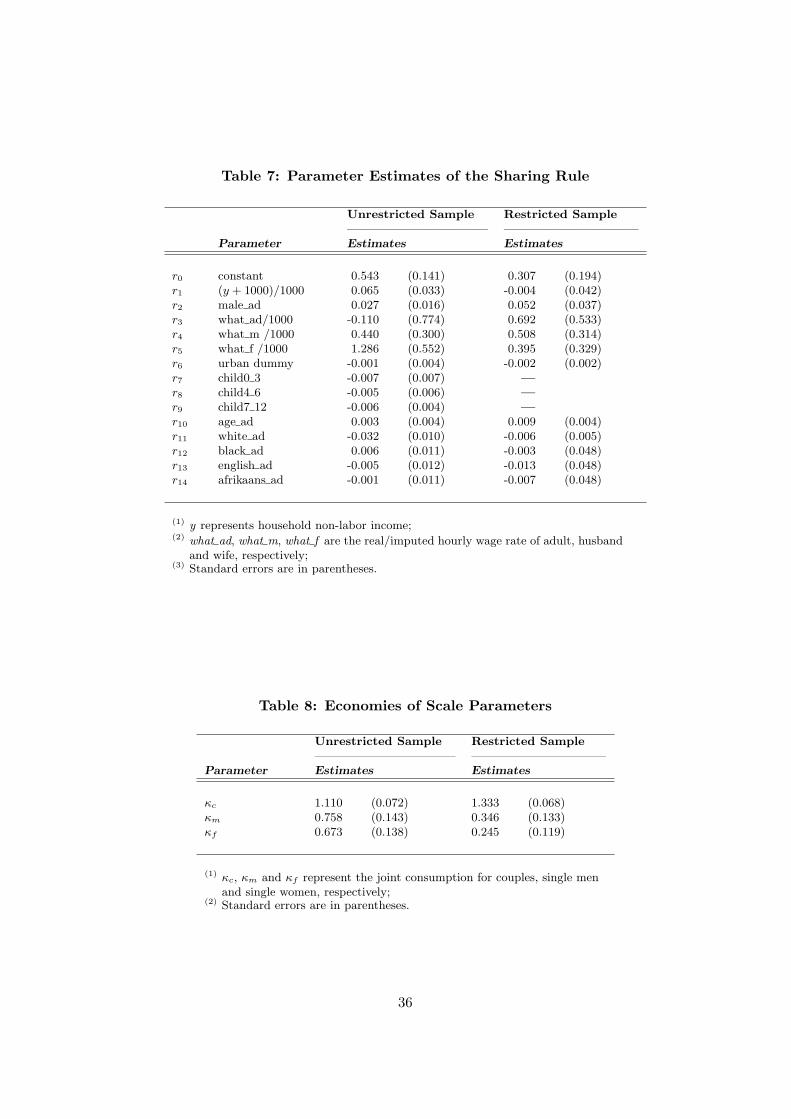
Table 7: Parameter Estimates of the Sharing Rule
Unrestricted Sample Restricted Sample———————————– ———————————
Parameter Estimates Estimates
r0 constant 0.543 (0.141) 0.307 (0.194)r1 (y + 1000)/1000 0.065 (0.033) -0.004 (0.042)r2 male ad 0.027 (0.016) 0.052 (0.037)r3 what ad/1000 -0.110 (0.774) 0.692 (0.533)r4 what m /1000 0.440 (0.300) 0.508 (0.314)r5 what f /1000 1.286 (0.552) 0.395 (0.329)r6 urban dummy -0.001 (0.004) -0.002 (0.002)r7 child0 3 -0.007 (0.007) —r8 child4 6 -0.005 (0.006) —r9 child7 12 -0.006 (0.004) —r10 age ad 0.003 (0.004) 0.009 (0.004)r11 white ad -0.032 (0.010) -0.006 (0.005)r12 black ad 0.006 (0.011) -0.003 (0.048)r13 english ad -0.005 (0.012) -0.013 (0.048)r14 afrikaans ad -0.001 (0.011) -0.007 (0.048)
(1) y represents household non-labor income;(2) what ad, what m, what f are the real/imputed hourly wage rate of adult, husband
and wife, respectively;(3) Standard errors are in parentheses.
Table 8: Economies of Scale Parameters
Unrestricted Sample Restricted Sample———————————– ———————————
Parameter Estimates Estimates
κc 1.110 (0.072) 1.333 (0.068)κm 0.758 (0.143) 0.346 (0.133)κf 0.673 (0.138) 0.245 (0.119)
(1) κc, κm and κf represent the joint consumption for couples, single menand single women, respectively;
(2) Standard errors are in parentheses.
36

Table A.1: List of the Variables of Interest
Variable name Definition of the variable
Male ad Dummy variable for male adults in single nuclear household.
Black iWhite i
Two dummies related to a person’s race.
Age i Dummy variable for whether individual i belongs to age category“18-40”.
Afrikaans iEnglish i
Two dummies defining the most often spoken languages.
Educ1 i ; Educ2 iEduc3 i ; Educ4 i
Dummy variables of i’s education level.
Child0 3Child4 6Child7 12
Dummy variables for children aged 0-3, 4-6 and 7-12, respec-tively.
Child0 3nChild4 6nChild7 12n
Number of children by category age: 0-3, 4-6 and 7-12, respec-tively.
Mother i Dummy for whether person i’s mother is alive.
Father i Dummy for whether person i’s father is alive.
Sister15 i Dummy for whether person i’s sister (aged 15 and more) is alive.
Adult nohh i Dummy for whether person i has at least one child alive and notliving in household.
Note: i ∈ (ad,m, f) represents the characteristics relative to single adults, married men and marriedwomen.
Table A.2: Average Household Size, Workers, Migrants, and Births by Pop-ulation Group
Sample All persons Persons above 15 Workers Migrants Births
Total 4.70 3.01 1.48 1.36 4.46
Black 4.94 3.07 1,38 1.36 4.76White 3.00 2.35 1.63 1.10 2.75Asian 4.43 3.37 1.79 1.09 3.62Colored 4.65 3.12 1.73 1.29 4.15
37

Table A.3: Job Type for People Aged 15 and More
Sample Full-time Part-time Casual No job
Total 26.56% 2.06% 1.25% 70.13%
Males 36.17% 1.99% 1.44% 60.40%Females 19.03% 2.11% 1.10% 77.76%
Black 21.92% 1.95% 1.10% 75.04%White 46.98% 2.85% 0.63% 49.55%Asian 40.49% 2.57% 1.26% 55.60%Colored 38.85% 2.11% 2.54% 56.50%
Note: People were asked if, during the last 7 days, they had a full-time, part-time or casual job. If the answer is NO, they are asked ifthey have actually a job from which they were absent the previousweek.
Table A.4: Employment Status of Working Age Population(Persons Aged Between 15 and 65)
Unemployment rate Participation rate
Sample Definition 1 Definition 2 Definition 1 Definition 2
Total 21.94% 38.04% 43.62% 54.94%
Males 17.48% 29.82% 53.86% 63.33%Females 27.36% 46.65% 35.43% 48.25%
Black 27.31% 46.18% 39.10% 52.80%White 4.01% 6.05% 61.64% 62.98%Asian 9.75% 12.95% 54.91% 56.93%Colored 14.28% 21.43% 57.19% 62.40%
(1) Definition 1 is the narrow definition of unemployment;(2) Definition 2 is the broader definition of unemployment that accepts as unemployed
those who did not search for work in a 4-week reference period but who report beingavailable for work and say they would accept if a suitable job were offered.
38
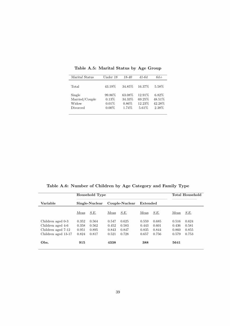
Table A.5: Marital Status by Age Group
Marital Status Under 18 18-40 41-64 64+
Total 43.19% 34.85% 16.37% 5.58%
Single 99.86% 63.08% 12.91% 6.82%Married/Couple 0.13% 34.33% 69.25% 48.51%Widow 0.01% 0.86% 12.23% 42.28%Divorced 0.00% 1.74% 5.61% 2.38%
Table A.6: Number of Children by Age Category and Family Type
Household Type Total Household—————————————————————————– ———————
Variable Single-Nuclear Couple-Nuclear Extended
Mean S.E. Mean S.E. Mean S.E. Mean S.E.
Children aged 0-3 0.352 0.564 0.547 0.625 0.559 0.685 0.516 0.624Children aged 4-6 0.358 0.562 0.452 0.583 0.443 0.601 0.436 0.581Children aged 7-12 0.951 0.895 0.843 0.847 0.835 0.844 0.860 0.855Children aged 13-17 0.824 0.817 0.521 0.728 0.657 0.756 0.579 0.753
Obs. 915 4338 388 5641
39
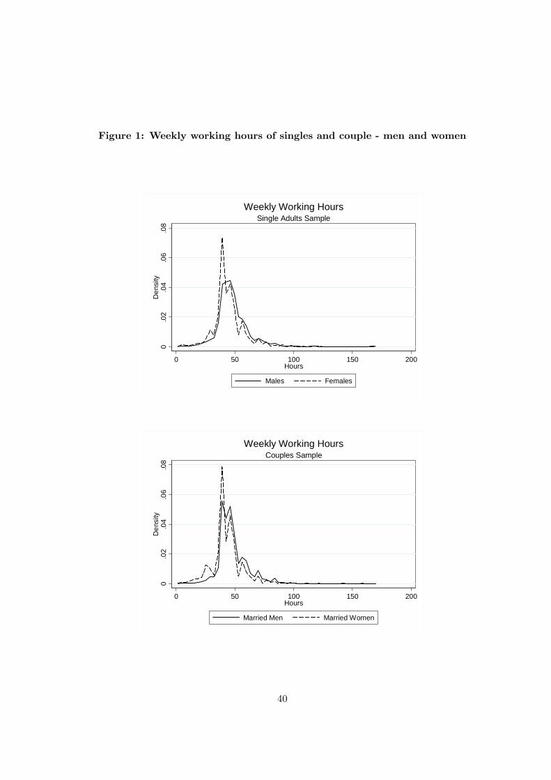
Figure 1: Weekly working hours of singles and couple - men and women
0.0
2.0
4.0
6.0
8D
ensi
ty
0 50 100 150 200Hours
Males Females
Single Adults SampleWeekly Working Hours
0.0
2.0
4.0
6.0
8D
ensi
ty
0 50 100 150 200Hours
Married Men Married Women
Couples SampleWeekly Working Hours
40

Figure 2: Sharing Rule Distribution
020
4060
Den
sity
.22 .24 .26 .28Single Adult Share
Unrestricted SampleDistribution of Adult's Share in Extended Households
020
4060
Den
sity
.08 .09 .1 .11 .12 .13Single Adult Share
Restricted SampleDistribution of Adult's Share in Extended Households
41