Embed Size (px)
Citation preview

1
Transfer Report
Yanting Shen
Trinity College
University of Oxford
Supervised by: Professor David Clifton
Professor Robert Clarke
Professor Zhengming Chen
25 September 2016

2
Abstract
We set out to use machine learning techniques to analyse ECG data to improve risk evaluation of
cardiovascular disease in a very large cohort study of the Chinese population. We performed this
investigation by (i) detecting “abnormality” using 3 one-class classification methods, and (ii)
predicting probabilities of “normality”, arrhythmia, ischemia, and hypertrophy using a multiclass
approach.
For one-class classification, we considered 5 possible definitions for “normality” and used
10 automatically-extracted ECG features along with 4 blood pressure features. The one-class
approach was able to identify abnormality with area-under- curve (AUC) 0.83, and with 75.6%
accuracy.
For four-class classification, we used 86 features in total, with 72 additional features
extracted from the ECG. Accuracy for this four-class classifier reached 75.1%. The methods
demonstrated proof-of-principle that cardiac abnormality can be detected using machine learning
in a large cohort study.
Our work contributes to the existing field of ECG risk evaluation by formulating a four-
class model for clinical integration of time-series data to electronic data records (EHR); proposing
a framework to reweight the posterior for an imbalanced training set; and proposing a framework
to evaluate the model against several “silver” standards when the “gold” standard is absent.
Related Publication
Shen, Y, Yang, Y, Parish, S et al., (2016). Risk prediction for cardiovascular disease using ECG
data in the China Kadoorie Biobank. EMBC 16: 38th Annual International Conference. (Accepted)

3
Table of Contents
Abstract .......................................................................................................................................... 2 Related Publication................................................................................................................................. 2
1. INTRODUCTION................................................................................................................. 4
2. MACHINE LEARNING FOR ECG RISK EVALUATION: EXISTING STUDIES .... 6 2.1 Feature extraction models ................................................................................................................ 6 2.2 Classification ..................................................................................................................................... 8 2.3 Other Machine learning models for time-series analysis ............................................................ 12 2.4 Conclusion ....................................................................................................................................... 13
3. DATASET DESCRIPTION ............................................................................................... 15 3.1 ECG time-series .............................................................................................................................. 15 3.2 ECG features ................................................................................................................................... 15 3.3 Blood pressure data ........................................................................................................................ 16 3.4 Textual labels .................................................................................................................................. 16 3.5 Health Insurance Data ................................................................................................................... 18
4. PREPROCESSING AND VISUALISATION .................................................................. 19 4.1 Feature Selection ............................................................................................................................. 19 4.2 Visualisation .................................................................................................................................... 20 4.3 Signal Quality Evaluation .............................................................................................................. 21 4.4 Feature Extraction .......................................................................................................................... 21
5. ANALYSIS .......................................................................................................................... 22 5.1 One-class classification ................................................................................................................... 22 5.2 Four-class classification ................................................................................................................. 26 5.3 Results and Discussion ................................................................................................................... 27
6. CONCLUSIONS AND FUTURE WORK ............................................................................ 31 6.1 Summary of work to date .............................................................................................................. 31 6.2 Immediate future work .................................................................................................................. 33 6.3 Plan until completion ...................................................................................................................... 39 6.4 Risk assessment ............................................................................................................................... 40
Appendix ...................................................................................................................................... 42 Appendix A: Gaussian Process Regression ........................................................................................ 42 Appendix B: The Gaussian Process Latent Variable Model ............................................................ 46 Appendix C: Support Vector Machines ............................................................................................ 48
Bibliography ................................................................................................................................ 52

4
1. INTRODUCTION
Cardiovascular disease (CVD), including coronary heart disease, cerebrovascular disease,
peripheral arterial disease, rheumatic heart disease, congenital heart disease, deep vein thrombosis,
and pulmonary embolism, is the leading cause of mortality worldwide [1] and in China [2]. An
estimated 3.76 million people died from CVD in China in 2013 [1]. There are large geographical
and economic variations of CVD mortality in China [2], suggesting appropriate measures may be
taken for prevention and effective treatment of the disease. For example, the World Health
Organisation advises people with high CVD risk to access early detection and management
facilities [1]. Studies have shown effective reduction of CVD mortality rates by promoting
awareness of risk factors and adopting lifestyle changes [1]. Identifying risks to the Chinese
population will help provide advice to people to improve their lifestyle and help clinicians to
discover appropriate treatments for specific conditions; this promises to reduce mortality and
healthcare expenditure. Many CVD risk factors have been identified by long-term follow-up
studies, such as obesity [3-5], diabetes [6], metabolic syndrome [7], smoking [1], and hypertension
[8], among many others. Recently, multiple biochemical and genetic risk factors have been
identified via conventional follow-up approaches, and by machine learning in large datasets [9].
While much research has been focusing on the effects of certain risk factors, personalised
medicine requires integrating all risk factors to which a person is exposed and then predicting risks
for specific diseases, so that preventative measures may be taken. Examples of research for this
purpose include [10], in which mathematical models were established by scoring systems using
multiple risk factors (blood pressure, total cholesterol, high-density lipoprotein cholesterol,
smoking, glucose intolerance, and left ventricular hypertrophy) as inputs to predict the risks of

5
myocardial infarction, coronary heart disease, CVD, and death from these diseases. With an
increasing number of risk factors being identified, and especially with abundant genetic and
lifestyle data now available, it can be expected that such an approach will face difficulty as the
“healthy” range of the newly-identified factors are hard to obtain or quantify.
Machine learning has the advantage of estimating the associations between risk factors and
diseases without prior knowledge of accurate reference values of the risk factors. This approach
has grown popular in risk evaluation and diagnostics for chronic diseases [11-14]. In CVD,
Knuiman et al. have predicted coronary mortality in the Busselton cohort using a discriminative
decision tree [15]; Lapuerta et al. used a neural network in the prediction of coronary disease risk
from serum and lipid profiles [16]; and Das et al. performed heart disease diagnosis using
ensembles of neural networks [17].
The electrocardiogram (ECG), being an important measurement of cardiac function that is
relatively easy to obtain, is surprisingly seldom used in prediction. This report attempts to address
the need for risk metrics that include ECG-derived features by analysing CVD risks associated
with abnormal ECG, using the China Kadoorie Biobank ECG dataset. This report includes two
risk evaluation tasks: (i) “abnormality” detection and (ii) prediction of probabilities of “normal”,
“arrhythmia”, and “ischemia”. Since abnormality is relatively rare in this database, novelty
detection (the aim of which is to classify an under-sampled “abnormal” class) is an appropriate
approach to address the first task. To address the second task we build models of “normality”,
“arrhythmia”, and “ischemia” on which probabilistic prediction of the “borderline” data will be
based.
This report includes a summary of existing studies on machine learning models for ECG

6
risk evaluation, followed by analysis of the two risk evaluation tasks. For the first task we compare
prediction performance of three one-class algorithms: (i) a generative KDE, (ii) a discriminative
KDE, and (iii) a discriminative SVM. They will be compared under five different assumptions for
the “normal” class. For the second task we propose a set of inclusion criteria for defining the four
classes corresponding to “normality”, “arrhythmia”, “ischemia”, “hypertrophy”, and present
classification accuracy using a support vector regression (SVR) with additionally extracted
features. Finally, the 4-class model was used to predict the “borderline” data which are not
assigned class membership, and compared with disease endpoints from the Health Insurance (HI)
dataset.
2. MACHINE LEARNING FOR ECG RISK
EVALUATION: EXISTING STUDIES
The typical 3-step framework for machine learning risk analysis with ECG data is 1) feature
extraction, 2) classification, and 3) model evaluation [9]. Risk evaluation tasks are usually
evaluated by how accurately the model predicts the labels that are used as the “gold standard”.
Examples of gold standards include human experts, and standard databases such as the MIT-BIH
arrhythmia database. Therefore, the literature involving risk analysis of ECG data is often referred
to as ECG classification, and the aim is to increase classification accuracy, sensitivity, and
specificity with respect to the gold standard.
2.1 Feature extraction models
For feature extraction, the most commonly used algorithms include the wavelet transform [17-19],
genetic algorithms for searching for candidate features [17], dynamic time warping (DTW) [20,
21], principle component analysis (PCA) [22], adaptions of the k-nearest neighbour (kNN)

7
algorithm for feature extraction [20], symbolic aggregate approximation (SAX) [20], correlation-
based feature selection [23], linear forward selection [23], power-spectrum methods [22],
Lyapunov exponents [18], fractal dimension [18], and morphology filtering [22], among many
others.
A classic example for improving classification accuracy is to discover novel patterns in
time-series [20], where Syed et al. improved risk stratification after acute coronary syndrome by
7 to 13% using three computational ECG biomarkers: morphologic variability (MV), symbolic
mismatch (SM), and heart rate motifs (HRM). MV, which quantifies the energy difference between
consecutive heart beats, was extracted by a process that included dynamic time warping to remove
the effect of time distortions in the ECG caused by respiration and other contributing physiological
factors. SM which measures the inter-patient difference was modelled via kNN novelty detection
after iterating a max- min clustering algorithm with a DTW distance metric. HRM was extracted
by symbolic aggregate approximation (SAX). These features are all unintuitive to human
inspection, but which were shown to be useful indicators of risk using the ECG.
Kim et al. proposed a robust arrhythmia classification algorithm using an extreme learning
machine, and used morphology filtering combined with PCA to classify 6 beat types [22]. Ye et
al. used morphological and dynamical features based on the wavelet transform and independent
component analysis (ICA) for classification of 16-class ECG beats [24]. They built decision
systems involving the fusion of results from two ECG leads, and reported 99.3% classification
accuracy.
El-Dahshan et al. used a hybrid involving genetic algorithms and wavelets to denoise the
ECG [17]. Goletsis et al. classified ischemic beats with a genetic algorithm which thresholds five

8
criteria describing ST segment changes, T wave alternans, and the patient’s age [25]. Their
sensitivity and specificity were both above 90%.
Arif et al. used the discrete wavelet transform to classify 6 beat types from ECG data with
99.5% accuracy, by using a KNN [26]; this work used PCA for feature reduction. Povielli et al.
proposed a novel approach that represents time-series data by a reconstructed phase space, and
tested the resulting feature space for use with arrhythmia and speech reorganization datasets; this
work used artificial neural network approaches [27].
2.2 Classification
For classification, the most commonly used classifiers include the support vector machine (SVM,
Appendix C) [19, 21, 22, 28-34], the multi-layer perceptron (MLP) [21-23, 34-36], the extreme
learning machine (ELM)[18, 22, 29] , random forests [34, 37], k-nearest neighbour (kNN) [21],
Bayesian decision making (BDM) [21], other artificial neural networks (ANNs) including aspects
of least-square methods (LSM) [21], polynomial classifiers [38], ensembles [39], fuzzy finite state
machines [40], stochastic Petri nets [40], decision trees [41], evolution algorithms [18], self-
organising maps [35], radial basis function networks [22], and straightforward linear regression
[34].
For example, Mitra et al. detected arrhythmia from ECG data using an incremental back
propagation neural network (IBPLN) and reported accuracy up to 87.7% [23]. They selected
features using correlation-based methods and linear forward selection. Fergus et al. predicted
preterm delivery of infants using a polynomial classifier on ECG and achieved 96% sensitivity,
90% specificity, and 95% AUC [38]. Tantimongcolwat et al. used a back-propagation neural
network (BNN) and a direct kernel self-organising map (DK-SOM) for detection of ischemic heart

9
disease on magneto-cardiograms (MCG), and achieved accuracy of to 80.4% on 125 individuals
[35]. Sun et al. achieved high performance in ECG classification with a reusable neuron
architecture (RNA) [36].
Kurz et al. developed a simple point-of-care risk stratification for acute coronary syndrome
(ACS) called “Acute Myocardial Infarction in Switzerland” (AMIS), and tested on 7520
participants. The study reported that the AMIS model outperformed several clinically-accepted
risk score systems [41]. Their classifier was based on Average One-Dependence Estimator (AODE)
and a J48 decision tree with a sequential backward deletion process for feature selection.
Hsich et al. used random survival forests to identify important risk factors for survival in
patients with systolic heart failure and achieved similar accuracy to a Cox proportional hazard
regression model; they found that the random forest offered more intuitive illustration of important
risk factors (and interactions between multiple risk factors) [37].
Arsanjani et al. used an ensemble-boosting algorithm to classify myocardial perfusion after
single- photon emission computed tomography (SPECT) for coronary artery disease in a large
population (n = 1181), and compared results with those from a clinically-used risk score involving
total stress perfusion deficit (TPD) and two human experts [39]. Their results outperformed TPD
and human experts in terms of ROC (0.94) and achieved at least as good sensitivity, specificity,
and accuracy.
2.2.1 The SVM as a robust classifier
The SVM has been shown to be particularly robust in many settings and has thus been used in
clinical studies either as the only classifier or as a comparison with the proposed algorithm. Its
mathematical formulation can be found at Appendix C. For example, Moavenin et al. improved

10
the basic SVM with a kernel-Adatron algorithm and compared to results from a MLP in the
classification of 6 arrhythmia beat types [42]. It was concluded that the SVM significantly
outperformed the MLP. Khorrani et al. used continuous wavelet transforms, discrete wavelet
transforms, and discrete cosine transforms for feature extraction; they performed arrhythmia
classification with an MLP and a kernel-Adaptron SVM using two-lead ECG [43]. This study also
confirmed that the SVM outperformed the MLP. Melgani et al. demonstrated the general
superiority of SVM compared to kNN and RBF networks in ECG classification, and improved the
SVM algorithm by using particle swarm optimisation (PSO); their study reported 89.7% accuracy
in the classification of 40,438 beats [44].
Similarly, Artis et al. conducted automated screening of arrhythmia using the discrete
wavelet transform. They trained two class classifiers (normal and arrhythmia) on the MIT-BIH
database and tested on a clinical cohort [45]. They reported that the highest accuracy was obtained
by an SVM, compared to an MLP and a Gaussian mixture model (GMM).
An SVM was used to classify signal quality of ECG and EEG, and achieved 92% accuracy
compared to human labels [30]. Khandoker et al. used an SVM to detect obstructive sleep apnea
syndrome (OSAS) from 8-hour ECG recordings and achieved 92.85% accuracy [31]. Kampouraki
et al. used an SVM for heart-beat time-series classification using long-term ECG recordings [32].
Bsoul et al. developed a real-time sleep apnea monitor, called “Apnea MedAssist”, which used an
SVM, and reported a sensitivity of 96% [33]. The algorithm requires only 1-minute ECG
recordings. Li et al. used an SVM to classify ventricular fibrillation and tachycardia classification
with 14 features [28]. They used a genetic algorithm for feature selection, and achieved 96.3%
accuracy, 96.2% sensitivity, and 96.2% specificity. Uebeyli et al. classified normal and partial
epilepsy from ECG using an SVM and achieved 99.44% accuracy, using wavelet coefficients as

11
features [19]. Yu et al. improved ICA for ECG beat classification by “independent component
rearrangement” and achieved 98.7% accuracy in 8 beat types using a probabilistic neural network
and a SVM [46]. Clifton et al. proposed a predicted and personalised multivariate early-warning
system using a one-class SVM and proposed a new way to parametrize the method for clinical
tasks using partial AUROC [47].
2.2.2 Classifiers outperforming SVMs
A number of models have been reported to outperform SVMs. For example, Özdemir et al. used
six machine learning classifiers (KNNs, LSMs, SVMs, Bayesian decision marking, dynamic time
warping, and ANNs) to detect falls from gyroscope, accelerometer, and magnetometer data [21].
They tested on a set of 2,520 trials comprising 20 voluntary falls and 16 types of daily living
activities. The best results were achieved by the KNN and LSM, with sensitivity, specificity, and
accuracy all above 99%.
Karpagachelvi showed that an extreme learning machine was superior to an SVM in ECG
classification because the former can optimise its parameters to best tune its discrimination of
classes, as well as identifying the best subset of features for the task [29]. Compared with the SVM,
another study concluded that methods such as MLPs, and RBF networks, and extreme learning
machine were more accurate and faster [22] for their task.
Zavar et al. reported that the SVM was outperformed by an evolutionary model in seizure
detection from ECG, in which feature extraction was performed via Lyapunov exponents, fractal
dimension, and wavelet entropy [18]. Monte-Moreno et al. estimated blood glucose and blood
pressure from the photoplethysmogram acquired from pulse oximeters with 410 participants using
ridge linear regression, MLPs, SVMs, and random forests, where the best result was achieved by

12
the latter [34].
2.3 Other Machine learning models for time-series analysis
Machine learning is readily applied to medical monitoring with time-series vital signs. For
example, Pullinger et al. implemented an automated system which calculates an early warning
score (EWS), and after implementing the automated system, the percentage of patients being
assigned an accurate EWS score increased from 52.7% to 92.9% [48]. In medical monitoring,
changes in time-series vital signs often indicate changes in underlying disease condition. Such
deviation from the “normal state” can be modelled by novelty detection approaches.
A Gaussian process (GP), which models the time-series as a distribution over functions, is
a one of the methods that are especially suitable to model the “normal state” for time-series data,
therefore we give a more detailed account here. The mathematical basics of GP can be found in
Appendix A.
Dürichen et al. proposed a multitask Gaussian process that can learn the correlation
between multiple vital signs [49]. The “abnormal state” can be classified by thresholding on the
resulting predicted risk scores using probabilistic extreme value theory (EVT) [50]. For example,
Clifton et al. generalised conventional univariate EVT for multivariate, multimodal problems [51],
and further extended the Generalised Pareto Distribution (GPD), which is followed by the extreme
values of any identical and independent distributed (i. i. d.) random variables from non-degenerate
distributions, to apply to high-dimensional data [52].
In [53], the “abnormality” in time-series was detected in a Gaussian process framework
using EVT. The functions from the output of a Gaussian process were mapped to probability

13
density z, then a distribution (𝑧) was defined over those densities; finally, an extreme function
distribution 𝐹(𝑟) was used to characterise the extremes of 𝐺(𝑧), where r is the Mahalanobis radius
from the “normal” model M. This approach showed the potential to classify “true” abnormality
from “extreme-but-normal” examples in time-series physiological data.
The strengths of Gaussian process regression include 1) the fact that it is a non-parametric
approach, and many other methods have been shown to relate to Gaussian process. For example,
relevant vector machines can be presented as a special case of a GP [54]; 2) The property that the
joint distribution is a Gaussian makes use of the convenient properties of Gaussian, i.e. the
conditional and marginal distributions are also Gaussian, which enables analytical solution in
many cases; 3) GP is intrinsically Bayesian, as shown in the inference of regression and
classification (Appendix A); 4) GP makes use of the so-called “kernel trick” which reduces
computational cost in many cases. An additional merit of GP for classification, compared to
probabilistic SVMs (which transforms some linear transformation of the discrimination boundary
through a sigmoid function) is that GP classification takes account into the predictive variance of
the latent function assumed to generate the data, 𝑓(𝒙). The main limitation of GP regression is that
the basic computational complexity is O(𝑛3), due to the inversion of an n by n matrix (where n is
the number of data), which therefore can be intractable for large datasets. Many approximation
strategies have been proposed for using GPs with large datasets, such as reduced rank
approximation of the Gram Matrix, greedy approximation, approximation with fixed
hyperparameters, and approximate the marginal likelihood and its derivatives. Details of
approximation algorithms can be found at chapter 8 of [54], and is omitted here.
2.4 Conclusion
There is a large body of literature concerning ECG classification, which reports high classification

14
accuracy, especially concerning arrhythmia classification. The SVM is reported as being one of
the most commonly-used and robust classifiers for ECG-based analyses, and is often used as a
point of comparison when a new model is proposed. Novelty detection approaches and algorithms
exploiting Gaussian process regression may be applied to ECG signal analysis for characterizing
the dynamical aspects of a time-series, which offers particular appeal in the setting of ECG analysis.
While these models yield high classification accuracy, they are mostly limited to a nearly-
balanced, small sample size chosen from distinctive groups labelled by clinical experts, and using
long ECG recordings. In comparison, the major challenges of our research include 1) a large
sample size (n = 25019) and short ECG recording length (t = 10s); 2) noisy labels due to a lack of
human expert labelling; 3) unbalanced classes with a large number of data points in the “middle
ground” between different classes; 4) the substantial time elapsed between clinical outcome and
ECG acquisition, as described in Chapter 3. These unique challenges pose the following research
questions that this research aims to address:
How should we integrate heterogeneous data types in the electronic health records (EHR),
and in particular, how should we handle the time-series data in a robust manner?
How should we handle datasets with heavily disproportional representation of classes?
With the absence of the “gold” standard, and the presence of several “silver” standards (as
is typical in clinical applications), how should we evaluate the models in a principled way?
In the following sections we will propose our solutions to the above questions, and, in the
conclusion and future work section, we will discuss ways to further provide more precise solutions
by using more advanced machine learning models.

15
3. DATASET DESCRIPTION
The China Kadoorie Biobank (CKB) is a prospective cohort study of over 520,000 adults from 10
areas in China during 2004-2008 [55]. Data were collected using questionnaires; physiological
measurements were recorded at baseline and all participants provided a blood sample. Information
on cause of death rates was collected from health insurance data, and from mortality and disease
registries. After five years, approximately 25,000 surviving participants were resurveyed with
further questionnaires, ECG measurements, and blood collection. We have institutional ethics
approval to use the data. Public access to the CKB data can be found at
http://www.ckbiobank.org/site/Data+Access.
The data available for our study include:
3.1 ECG time-series
Standard 12-lead ECG (10-s duration, 500Hz) was recorded on 24,369 participants using a Mortara
ELIx50 device in 2013-2014. Also available is a “typical cycle” from each lead for each participant,
which was generated by the device using a proprietary algorithm.
3.2 ECG features
The Mortara device provides 19 features (Table 2) which were automatically extracted from the
“typical cycles” for each participant. A schematic representation of a selection of these features is
shown in Figure 1.

16
Figure 1 Schematic representation of key ECG features for Lead I
3.3 Blood pressure data
Systolic blood pressure and diastolic blood pressure were recorded twice on each individual using
standard methods.
3.4 Textual labels
The Mortara device automatically provides up to 10 textual labels from 236 possibilities for each
participant, such as sinus rhythm, normal ECG, and atrial fibrillation. These labels were produced
by application of the Minnesota coding system which is a heuristic scheme defined [56]. Sinus
rhythm and normal ECG are the most commonly-observed textual labels in our dataset,
representing 83.2% and 44.1% of all records, respectively.
The outputs of the Mortara device included a label for abnormality for the waveform
(abnormal ECG), which was coded as 1 for abnormality and 0 for normality.
3.4.1 Labels for one-class novelty detection:
Sinus rhythm, normal ECG, and abnormal ECG=0 were the only three labels available in our
dataset that were used as potential criteria for defining normality. There were 19,925, 10,550, and
17
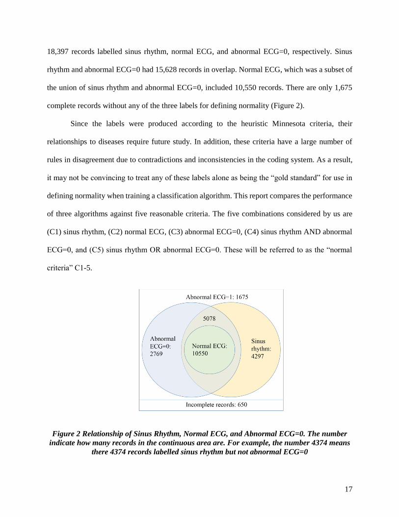
18,397 records labelled sinus rhythm, normal ECG, and abnormal ECG=0, respectively. Sinus
rhythm and abnormal ECG=0 had 15,628 records in overlap. Normal ECG, which was a subset of
the union of sinus rhythm and abnormal ECG=0, included 10,550 records. There are only 1,675
complete records without any of the three labels for defining normality (Figure 2).
Since the labels were produced according to the heuristic Minnesota criteria, their
relationships to diseases require future study. In addition, these criteria have a large number of
rules in disagreement due to contradictions and inconsistencies in the coding system. As a result,
it may not be convincing to treat any of these labels alone as being the “gold standard” for use in
defining normality when training a classification algorithm. This report compares the performance
of three algorithms against five reasonable criteria. The five combinations considered by us are
(C1) sinus rhythm, (C2) normal ECG, (C3) abnormal ECG=0, (C4) sinus rhythm AND abnormal
ECG=0, and (C5) sinus rhythm OR abnormal ECG=0. These will be referred to as the “normal
criteria” C1-5.
Figure 2 Relationship of Sinus Rhythm, Normal ECG, and Abnormal ECG=0. The number
indicate how many records in the continuous area are. For example, the number 4374 means
there 4374 records labelled sinus rhythm but not abnormal ECG=0

18
3.4.2 Labels for four-class classification:
For 4-class classification of “normal”, “arrhythmia”, “ischemia” and “hypertrophy”, it is
important to construct class models as precisely as possible. We also require criteria for the 4-class
setting, and here we consider schemes according to [57] which are shown in Table 1.
Table 1 Four class inclusion criteria and class sizes
3.5 Health Insurance Data
The Health Insurance data of 25,001 out of the 25,019 participants were also available, which
includes 5 versions of 80 endpoints. The 5 versions each represents a data source: death certificates,
underlying cause of death from death certificates, routine disease report data, health insurance
event data, and any of the above. The endpoints are disease classes and sub-classes, including
vascular disease, malignant neoplasms, disease of the respiratory system, infectious and parasitic
disease, diabetes, liver cirrhosis, chronic kidney disease, stroke, disorders of the eye lens, and
external causes. These endpoints happened prior to ECG acquisition, for up to 5 years. The time
of onset of these causes were also provided, as well as 1,126,619 procedures (ranging from
“dimming the light on the ward” to surgery) associated with these causes. Due to the sparsity of
the data, cardiovascular diseases from all data sources were used as labels to compare with the
Class Number (%) Inclusion criteria
Normal 10803 (43.2) Normal ECG
Arrhythmia 2162 (8.6) Abnormal rhythm, atrial
fibrillation, early
repolarization, preexcitation,
premature ectopic beats,
ectopia, blocks, uncertain
rhythm
Ischemia 1868 (7.5) Explicitly stated “ischemia”
Hypertrophy 3761 (15.0) Hypertrophy or enlargement
Unclassified 6425 (25.7) None of the above

19
model predictions.
4. PREPROCESSING AND VISUALISATION
4.1 Feature Selection
Table 2 Mortara features and 4 blood pressure features. Features are excluded either because
they can be expressed as functions of other features or because they are constant
Included features Explanation
Age
Average RR interval
QRS offset
P wave duration
PR interval
QRS duration
QT duration
P axis
QRS axis
T axis
SBP first
SBP second
DBP first
DBP second
Average distance between two R peaks
End of the QRS complex
Interval between Q wave onset and T wave offset
Determined by deflects of P wave in different leads
Interval between Q wave onset and T wave offset
Determined by deflects of P wave in different leads
Determined by deflects of QRS wave in different leads
Determined by deflects of T wave in different leads
Systolic blood pressure in the first resurvey
Systolic blood pressure in the second resurvey
Diastolic blood pressure in the first resurvey
Diastolic blood pressure in the first resurvey
Excluded Features
Ventricular rate
R peak
P wave onset
P wave offset
QRS onset
T wave offset
𝑄𝑇𝑐 duration
𝑄𝑇𝑐𝐵 duration
𝑄𝑇𝑐𝐹 duratiob
=60000
𝐴𝑉𝑒𝑟𝑎𝑔𝑒 𝑅𝑅 𝑖𝑛𝑡𝑒𝑟𝑣𝑎𝑙
always at 500ms
= 𝑄 𝑜𝑓𝑓𝑠𝑒𝑡 − 𝑃𝑅 𝑑𝑢𝑟𝑎𝑡𝑖𝑜𝑛 − 𝑄𝑅𝑆 𝑑𝑢𝑟𝑎𝑡𝑖𝑜𝑛
= 𝑃 𝑜𝑛𝑠𝑒𝑡 + 𝑃 𝑑𝑢𝑟𝑎𝑡𝑖𝑜𝑛
= 𝑃𝑅 𝑑𝑢𝑟𝑎𝑡𝑖𝑜𝑛 + 𝑃 𝑜𝑛𝑠𝑒𝑡
= 𝑄 𝑜𝑛𝑠𝑒𝑡 + 𝑄𝑇 𝑑𝑢𝑟𝑎𝑡𝑖𝑜𝑛
=𝑄𝑇 𝑑𝑢𝑟𝑎𝑡𝑖𝑜𝑛
√𝑎𝑣𝑒𝑟𝑎𝑔𝑒 𝑅𝑅 𝑖𝑛𝑡𝑒𝑟𝑣𝑎𝑙
=𝑄𝑇 𝑑𝑢𝑟𝑎𝑡𝑖𝑜𝑛
(𝑎𝑣𝑒𝑟𝑎𝑔𝑒 𝑅𝑅 𝑖𝑛𝑡𝑒𝑟𝑣𝑎𝑙)1/3
Of the 19 features available from the Mortara device, 9 were excluded because they can be
expressed as functions of other features or because they have constant values. These are shown in

20
Table 2. We removed records with missing values for any of the features, and data for 24,369
participants were thus retained for use in our study.
4.2 Visualisation
We performed a 2-D visualisation of the 14-dimensional feature space according to the 5 normal
criteria, C1-C5, using a Gaussian process latent variable model (GPLVM), which projects high-
dimensional data into a lower-dimensional subspace. See appendix B for mathematical details.
Here we use GPLVM instead of Principle Component Analysis (PCA) because PCA assumes
linear relation of the latent variables and the observed variables, while we prefer to relax this
assumption by using a dimension reduction method that can capture nonlinear relations. It may be
seen from figures 3 that substantial overlap exists between the “normal” and “abnormal” classes,
and among normal, arrhythmia, ischemia, and hypertrophy classes, as is expected for a complex,
realistic medical application.
Figure 3 2-D visualisation of 500 normal and 500 abnormal data randomly selected according
to the criteria C5 (left) and 100 data points randomly selected from each of the four classes
(right)

21
4.3 Signal Quality Evaluation
A Signal Quality Index (SQI) was evaluated for all 12-lead ECG signals independently using in-
house software [58]. The SQI ∈ [0, 1], depends on the agreement of two peak detectors concerning
the positions of the R-peaks. Close agreement yields a high SQI, which corresponds to high signal
quality.
97.11% of all 12-lead waveforms were deemed to be of high quality (SQI≥0.9). Each lead
has at least 92% data with SQI≥0.9. Lead V4 has the highest proportion (99.2%) of good-quality
signals (SQI≥0.9). The signal quality of our dataset is therefore deemed to be sufficient to classify
at least 92% of the 24,369 participants with complete ECG records.
4.4 Feature Extraction
6 additional features are extracted from the “typical cycles” from each of the 12 leads: amplitudes
of P, Q, R, S, and T waves relative to the baseline, and ST level (which was approximated as the
level of the ECG observed at the time given by the QRS offset). The baseline was approximated
as the average level of the segment between P offset and Q onset, because this segment is used to
define ST deviation in the clinic. The positions of the onsets and offsets of these waves are
provided by the Mortara device (part of the Mortara features, Figure 4).

22
Figure 4 Schematic plot of the new features defined by us (red stars): amplitudes of P, Q, R,S,
T waves, and ST level. The occurrence of onsets and offsets of these waves are given by the
Mortara device and are shown by the blue arrows.
5. ANALYSIS
5.1 One-class classification
We present three methods to predict the posterior probability of a feature vector belonging to the
abnormal class, and hence predict their cardiovascular disease risk. The entire analysis process is
illustrated in Figure 5, and is described in detail as follows:
5.1.1 Cross-validation and partitioning of training and test sets
We performed 5-fold cross-validation by permuting the entire dataset and assigning a different 20%
for each fold of cross-validation. Results shown later are the mean values over this 5-fold cross-
validation. All sets were normalised column-wise according to the mean and standard deviation of
the training set.
5.1.2 Balancing of the test sets
To make a fair comparison between the normal criteria C1-C5 which have different class ratios
(i.e. balance between normal and abnormal data), we used the accuracy in balanced sets and AUC

23
in both balanced and unbalanced sets for model evaluation.
We therefore created a balanced test set (a subset of the unbalanced test set), containing all
abnormal test data and the same number of normal data. The training set remained unbalanced.
Figure 5 Analysis framework for one-class classification

24
5.1.3 Statistics
The definitions we used for accuracy, true positive rate (TPR), and false positive rate (FPR) are:
𝑎𝑐𝑐𝑢𝑟𝑎𝑐𝑦 =𝑇𝑃+𝑇𝑁
𝑇𝑃+𝑇𝑁+𝐹𝑃+𝐹𝑁 (1)
𝑇𝑃𝑅 =𝑇𝑃
𝑇𝑃+𝐹𝑁 (2)
𝐹𝑃𝑅 =𝑇𝑃
𝑇𝑃+𝐹𝑁 (3)
where TP: true positive, TN: true negative, FP: false positive, FN: false negative.
5.1.4 Generative KDE
We adapted the model described in [50]. In brief, the “normal” class probability density
function (pdf) was learned from the training set by placing a multivariate Gaussian distribution on
each 14-dimensional data point. For ease of computation, we performed k-means clustering to
summarise the “normal” data with 500 cluster centres in the 14-dimensional space. Only the most
“normal” (i.e., those labelled “normal ECG”) were used in clustering. The data likelihood is
calculated via:
𝑝(𝒙) =1
𝑁(2𝜋)𝐷2 𝜎𝐷
∑ 𝑒−
|𝒙−𝒙𝑖|2
2𝜎2𝑁𝑖=1 (4)
A novelty score, y, is then calculated using equation 5.
𝑦(𝒙) = − log 𝑝(𝒙) (5)
We propose treating this novelty score as a univariate summary of the 14-dimensional data,
which may then subsequently used by probabilistic models to predict the probability of test data
belonging to the abnormal class. First we learn the likelihood 𝑝(𝑦|𝐶) in the training set, by
performing a kernel density estimation of the class-specific pdf. For the unbalanced test set, the

25
prior P(C) is set to the class ratio of the training set; for the balanced set, the class prior equals 0.5.
The posterior is
𝑝(𝐶|𝑦) =𝑝(𝑦|𝐶)𝑝(𝐶)
𝑝(𝑦) (6)
The posterior 𝑃𝑡𝑒𝑠𝑡(𝐶|𝑦) is thresholded at 0.5 for classification.
5.1.5 Discriminative KDE
Alternatively we can feed the novelty score into a discriminative framework by solving the
inference problem 𝑝(𝐶|𝑦) directly [59]. The posterior is learned in the training set by binning y
and calculating the frequency of observing a particular class in a bin (figure 6). For example, for
“normal” class C0, the posterior in each bin is calculated as the proportion of data points belonging
to C0 in that bin. Ideally, the bin size should be determined by cross-validation [50]. In this report,
the bin size was set to y = 1. The posterior of a set with a different prior, in this report the balanced
test set, is calculated according to equation 7. Similarly, the posterior is thresholded at 0.5 for
classification.
Figure 6 Learning the posterior by binning the novelty score y. the distribution of y was
binned and in each bin the frequency of observing the class C was calculated to estimate the
posterior in the training set.

26
𝑃𝑡𝑒𝑠𝑡(𝐶|𝑦) =𝑃𝑡𝑟𝑎𝑖𝑛(𝐶|𝑦)𝑃𝑡𝑟𝑎𝑖𝑛(𝑦)𝑃𝑡𝑒𝑠𝑡(𝐶)
𝑃𝑡𝑟𝑎𝑖𝑛(𝐶)𝑃𝑡𝑒𝑠𝑡(𝑦) (7)
5.1.6 Discriminative SVM for one-class classification
To compare the results of KDE we also used an SVM. See appendix C for mathematical
formulations of SVM. Here we use Gaussian kernel and select the coefficients C and σ by grid
search via 5-fold cross-validation on the training set. The classification score is mapped to
probabilities and thus the training set posterior 𝑝(𝐶|𝑦) is learned. For an unbalanced test set, the
posterior is estimated to be equal to the training set, while the balanced test set posterior is
reweighted using equation 7.
5.2 Four-class classification
5.2.1 Constructing the training and test sets
We obtained balanced training and test sets by taking all data from the smallest class (Table 1),
and the same number of data points from each of the other classes were randomly selected to
construct the training and test sets for 5-fold cross-validation. For example, the four-class balanced
training-and-test set contains 1868 × 4 = 7472 datapoints. To illustrate the distinctiveness of each
class, three-class and two-class classifications of any combinations of the “normal”, “ischemia”,
“arrhythmia”, and “hypertrophy” were also performed for comparison using the same approach to
balance classes.
5.2.2 Training the 4-class model
A 𝑃(𝐶|𝑦) was estimated for each of the classes using support vector regression (Appendix C) in
a one-vs-all approach; i.e. the regressor 𝑖 was learned in a training set with only the class 𝑖 labelled

27
1 and other classes were labelled 0. The class probability 𝑃(𝐶|𝒙) was calculated from the predicted
value of the regressor i according to equation 8 (See Appendix C for the derivation of this equation).
Finally the data point was classified to the class i which maximises the probability:
𝑃𝑖(𝐶𝑖|𝒙) =𝑒
−|1−𝑦𝑖|
𝜎𝑖
2𝜎𝑖 ∑ 𝑃𝑗(𝐶𝑗|𝒙)4𝑗=1
, 𝑖 = 1,2,3,4 (8)
5.2.3 Risk prediction
The 4-class model were used to predict the 24,344 participants with complete features in the health
insurance dataset, using cardiovascular endpoints from all data sources for comparison. All
participants predicted as arrhythmia, ischemia, or hypertrophy were included in the “Predicted
CVD” class.
5.3 Results and Discussion
5.3.1 One-class classification
Under all 5 criteria C1-C5, data from the normal class take overall lower novelty scores than data
from the abnormal class, as shown in figure 7. However, the two classes are largely overlapped in
the peak area of the abnormal class, suggesting that the generative KDE may not be able to separate
them easily. Figure 7 shows the likelihood under the criteria C5, and the results for other criteria
were similar.

28
Figure 7 Likelihood using the normal criteria on C5
In order to rule out the influence of different test sets to classification accuracy, we first
evaluated the performance of the discriminative SVM and generative KDE with the same
(unbalanced) test set. Considering the substantiate overlap shown by the visualisation (Figure 3)
and the likelihood (Figure 7), the generative KDE and discriminative SVM have relatively high
AUC. Under criterion C5, the AUC is high for both methods. The SVM model achieved higher
AUC for all criteria, suggesting it may be a more robust method than the KDE (Figure 8 and Table
3).
Table 3 AUC under normal criteria C1-C5 in the same test set
Normal
Criteria
C1 C2 C3 C4 C5
SVM
KDE
0.82
0.73
0.78
0.73
0.79
0.73
0.80
0.75
0.80
0.79

29
Figure 8 ROC curves of the same unbalanced test set under the five normal criteria
Using the balanced set, the discriminative SVM achieved high accuracy, 71.1% to 75.6%,
for all 5 criteria, while the generative KDE has a comparable result (74.8%) using criterion C5
(Table 4). The discriminative KDE has similar AUC values as the generative KDE, but lower
accuracy, which implies a better optimisation of this method may be needed. Figure 8 shows that
the most distinctive normal criterion is different for each method. For the generative KDE and the
discriminative SVM the best-performing criterion is C5, and C1, respectively, suggesting different
algorithms may favour different criteria.
Table 4 AUC and Accuracy of predicting the 5 normal criteria by generative KDE,
discriminative KDE, and discriminative SVM in the balanced sets.
Discriminative SVM Generative KDE Discriminative KDE
AUC Accuracy % AUC Accuracy % AUC Accuracy %
C1
C2
C3
C4
C5
0.79
0.79
0.82
0.80
0.83
71.7
71.6
77.1
73.7
75.6
0.73
0.73
0.72
0.75
0.81
67.2
63.5
65.1
64.5
74.8
0.73
0.73
0.72
0.75
0.80
59.6
61.1
59.3
61.4
60.6

30
It is unexpected that the most stringent criterion, C3, being the subset of all other 4 criteria,
has not yielded best results with any of the algorithms considered. The criterion C5 is predicted
accurately by both the generative KDE and the discriminative SVM, suggesting that it may be
more appropriate for use as the “gold standard” for training algorithms for one-class classification.
5.3.2 Four-class classification
The four-class classification results using support vector regression are shown in Figure 9.
Accuracies between the two classes on the nodes; numbers in the centres of the triangle are
classification accuracies of the 3 classes on the nodes of the triangle. The red and black numbers
are results with and without the 72 features derived from the ECG, over and above the basic set of
the 10 features provided by the Moratra device and the 4 blood pressure features, respectively.
The 72 new features improved the results in all cases, most markedly in classifications
involving ischemia and hypertrophy. This agrees with our expectation since the 10 Mortara
features do not contain information concerning the amplitudes of the peaks, while ischemia and
hypertrophy were highly correlated with amplitude abnormalities, especially ST-levels, and R-S
amplitudes.
It is encouraging that the classification accuracies with the new features are 30 to 50
percentage points higher than those that would be obtained by chance, suggesting machine learning
methods can achieve high agreement with clinical knowledge, without resorting to a complex rule-
based system.
In comparison with the HI dataset endpoints, 8,597 participants who were labelled CVD
negative in the HI dataset were predicted with CVD, while 1607 participants labelled CVD positive

31
were predicted as being “normal”. The substantial time difference between ECG acquisition and
the endpoint onsets (as well as the short duration of the ECG recordings) are major contributors to
this discrepancy. It is possible that participants may have developed or recovered from CVD during
the time elapsed between the label in the health insurance dataset and the acquisition of ECG data.
Figure 9 Classification accuracies (see the text for description)
Table 5 Comparison of predicted CVD with health insurance records
Predicted CVD Predicted Normal
CVD positive
CVD negative 1882
8597
1607
12258
6. CONCLUSIONS AND FUTURE WORK
6.1 Summary of work to date
We have addressed the task of risk evaluation using ECG of about 25,000 participants by (i)
building three novelty detection (one-class classification) models to detect abnormality with a
generative KDE, a discriminative KDE, and a discriminative SVM, and (ii) a 4-class model for

32
probabilistic risk prediction of normal, arrhythmia, ischemia, and hypertrophy using 82 features
extracted from ECG times series and 4 blood pressure data from about 25,000 participants, using
support vector regression. We tested the validity of our one-class and four-class models with
Mortara labels (i.e., those from a complex, heuristic clinical algorithm). Subsequently we used our
four-class model to predict four-class probabilistic risk scores on the same cohort, and then
compared our results with their disease history in the health insurance dataset.
Specially, to address the second research question proposed at the end of section 2, we have
proposed a framework that reweights the posterior trained in a highly unbalanced training set. This
method is especially desirable in novelty detection, where balancing the training set means loss of
the majority of the data.
The first task of this research was to detect “abnormality”, by exploring different one-class
novelty detection algorithms under various criteria of “normality”. The algorithms favoured
criteria C5, which was the least stringent of all possibilities. In view of the relatively good
performance of the discriminative SVM, in the second task of this study we modelled the “normal”,
“arrhythmia”, “ischemia”, and “hypertrophy” using multiclass support vector regression, aiming
to produce accurate models for prediction of the unclassified data points according to the labels.
The encouraging results suggest the multiclass models may be appropriate to predict the
probability of class membership of the “borderline” data that are otherwise difficult to classify.
We can further improve the classification accuracy by extracting more features, such as heart-rate
variability and T-wave alternans.
Our novelty detection task is not a typical supervised machine learning problem, due to the
absence of the “gold” standard. We proposed systematical evaluation of the model against all

33
“silver” standards, and base our evaluation on the assumption that if our predictions are sufficiently
close to the silver standards, they are also sufficiently close to the latent “gold” standard.
The 𝑃𝑖(𝐶𝑖|𝒙) in the four-class model (eq. 8) used in classification is actually a “pseudo-
posterior”, because it was calculated from the probability of regression scores, whose pdf was
calculated in a parametric approach (via the Laplace distribution). The regression score itself does
not have a probabilistic interpretation, and we can make the model more mathematically sound by
calculating the “true posterior” according to eq. 6 and predict four probabilistic risk scores for each
participants. Also, the four classes (normal, ischemia, arrhythmia, and hypertrophy) are treated as
independent so far. With a “true posterior” we can produce conditional risk scores based on any
relationships that may exist between the four classes.
The original 10s signal may lend more information than the “typical cycle” as the former
contains more time-dependent information than the latter. The length of the signal is a major
limitation to our feature extraction, because many informative features such as ST-level need
longer (> 60s) signals to be evaluated accurately [60]. Features may be extracted from the 10s
signal using recurrent neural networks (RNN) and compared with clinical indices such as the
Sokolow Index [61]. Future work will link our analysis of ECG data to other epidemiology data
such as body mass index (BMI), blood pressure, and stroke risk scores available via the China
Kadoorie Biobank.
6.2 Immediate future work
6.2.1 Further analysis
Our immediate future work will include (i) performing additional analyses with existing models
to better compare with the literature, reporting on metrics that would permit direct comparison; (ii)

34
producing Bayesian probabilistic risk scores to introduce “rejection options” (e.g., “cannot
classify”) and conditional risk scores; and (iii) comparing our features with the clinical-standard
Sokolow index [62] to evaluate the improvement to this well-understood but simplistic existing
method, and iv) conceptualise our framework of evaluating against multiple “silver” standards
with the absence of the “gold” standard using latent variable model. We denote the latent “gold”
standard 𝑍 = {𝑧𝑛}, and the noisy obervations of 𝑍, i.e. the silver standards as 𝑇 = {𝑡𝑛𝑘}, with the
superscript indexing the “silver” standards and subscript indexing the participant, and model
𝑃(𝑇|𝑍) using appropriate parametric (for example multinomial) or nonparametric models, and
study the joint distribution 𝑃(𝑋, 𝑇), where 𝑋 is data matrix.
We will also perform a retrospective analysis taking advantage of the occurrence time of
the diseases in the health insurance data, to illustrate how our prediction improves as we exclude
distant evets from ECG acquisition, and further validate our models in the time domain. These
tasks will likely be completed by December 2016, when we will discuss with our clinical
collaborators about ways to communicate the results of our research to a clinical audience for
publication in the epidemiological literature.
6.2.2 Epidemiology analysis
We will correlate our results with blood pressure, and subsequently after data acquisition, with
body mass index (BMI) and stroke risk scores, to evaluate the contribution of our risk scores to
risk stratification. We will then build robust electronic health record (EHR) models with
heterogeneous data in the CKB database. The latter will involve consideration of probabilistic
models that permit the fusion of categorical data, and which may include sparse techniques for
handling the largely-incomplete records in the dataset. These studies will likely be conducted

35
during Michaelmas Term 2016/2017.
6.2.3 “Omics” data analysis
We will then analyze the genomics and proteomics data in the CKB database. These will be
continuous or categorical data and can be explored by various machine learning models, including
Bayesian non-parametric “Indian buffet processes” for matrices of sparse binary data. Comparison
will be performed with appropriate kernel methods, such as sparse logistic kernel machines. We
will incorporate our ECG risk scores with -omics data to create comprehensive risk scores,
potentially for more disease types than we have initially considered, such as cancer and stroke.
These will likely be conducted from Michaelmas to Hilary Term of 2016/2017.
6.2.4 Deep learning models for ECG analysis
Cardiac activity is a dynamic system which can be accurately modelled by recurrent neural
network (RNN), which differs from feedforward neural network in that there are loops in directed
graphs (Figure 10, courtesy [63]). Funahashi et al. proved that an arbitrary dynamic system can
be modelled accurately by a continuous recurrent neural network (RNN) [64]. However, the main
difficulty in training the RNN is that the conventional backpropagation algorithm requires acyclic
structure, thus cannot be applied directly to RNN. Many algorithms have been proposed for
training of RNN, including BPTT [65, 66], real time recurrent learning (RTRL) [67], etc. However,
they suffer from ‘blowing-up’ or ‘vanishing’ back error derivatives, thus conventional RNN
doesn’t perform well when the time elapse required in the short-term memory is relatively long.
This problem was studied intensively in [68]. Mathematically, Hochreiter et al. gave the local scale
factor between error gradients of arbitrary unit 𝑢 at time point 𝑡 back prop to unit 𝑣 at time 𝑡 − 𝑞
is:

36
∂𝓋v(t−q)
∂𝓋u(t)= ∑ …n
l1=1 ∑ ∏ flm′(netlm(t − m))wlmlm−1
qm=1
nlq−1=1 (9)
where
𝓋k(t) = {fk
′(netk(t))(dk(t) − yt(t)), k is output unit
fk′(netk(t)) ∑ wik𝓋ki (t + 1), k is nonoutput unit
(10)
is the error of arbitrary unit 𝑘 at time point 𝑡, where dk(t) is the target at time 𝑡 for unit 𝑘, if 𝑘 is
an output unit, and
yi(t) = fi(neti(t)) (11)
is the activation of a non-input unit 𝑖 with activation function fi, and
neti(t) = ∑ wijyj(t − 1)j . (12)
If
|flmj(netlm(t − m))wlmlm−1| > 1.0 (13)
the error gradient will explode by the end of backpropagation;
If
|flmj(netlm(t − m))wlmlm−1| < 1.0 (14)
the error gradient will vanish.
Thus to ensure the parameters can be properly learned the gradient must satisfy
|flmj(netlm(t − m))wlmlm−1| = 1.0 (15)
In other words, a simple recurrent neural network (SRN) has only a simple recurrent unit
in its hidden layers which is usually a sigmoidal function (figure 10 left), and because of the
product of multiple sigmoid functions will flatten, an effective RNN structure must contain
addition operations. Hochreiter et al. [69] proposed long short-term memory (LSTM) which
features gated cells instead of the simple recurring unites in SRN. One of the most commonly used
LSTM structure nowadays is the so-called ‘Vanilla network’ proposed by Graves and

37
Schmidhuber [70]. We follow the presentation in [63] and present the illustration (courtesy [63])
and mathematical formulation as follows:
Figure 10 Detailed schematic of the Simple Recurrent Network (SRN) unit (left) and a Long
Short-Term Memory black (right) as used in the hidden layers of a recurrent neural network.
in which
zt = g(Wzxt + Rzyt−1 + bz) (16)
it = σ(Wixt + Riy
t−1 + pi⨀ct−1 + bi) (17)
f t = σ(Wfxt + Riy
t−1 + pf⨀ct−1 + bf) (18)
ct = it⨀zt + f t⨀ct−1 (19)
ot = σ(Woxt + Royt−1 + po⨀ct + bo) (20)
yt = ot⨀h(ct) (21)
where 𝑊 denote the weight matrix for input 𝑥, 𝑅 is the square matrix linking recurrent units, 𝑏 is
the bias vector, 𝑝 is the peephole vector which can be used to make variations on the structure,
with the simplest structure being a unit vector, and functions σ, 𝑔 and ℎ are point-wise non-linear
activation functions: logistic sigmoid is used for as activation function of the gates 𝑖, 𝑜, 𝑓, and

38
hyperbolic tangent is usually used as the block input 𝑧 and output activation function 𝑦.
Central to the LSTM structure is the addition operation which forces constant error carousal
(CEC, equation 15). The input and block output from other memory cells in the hidden layers are
not only fed into the cell state, but also to each of the three gates. In learning phase all 𝑊, 𝑅, and
𝑏 are to be learned, which is analogous to training each memory cell to forget, input, or output
when appropriate. The LSTM net was shown to be able to effectively retain memory of 1000 time
steps [69]. The classic applications of LSTM are on sequential data in which previous data are
informative to the latter data, such as in natural language processing and polymorphic music
modelling, and LSTM is arguable the most effective and efficient algorithm for predicting
sequential data [71]. We refer to [72] for PhD thesis on LSTM, [73] for PhD thesis on training
RNN, [74] for applying LSTM on sequential data, [75] for application on image generation, and
[76] for gated feedback RNN. Helpful tutorials can be found at http://deeplearning4j.org/lstm and
http://people.idsia.ch/~juergen/rnn.html, and open-source software packages can be found at
http://people.idsia.ch/~juergen/rnn.html.
We conclude that the LSTM is appropriate for modelling time-series medical data, yet there
has not been such a study reported in the literature. One way to model ECG, for example, is to use
a subset of “normal” ECG signal as a training set, in which the ECG signal is the input x, prediction
of time point 𝑡 later than 𝑥 being 𝑦(𝑡); this allows us to quantify the divergence of prediction 𝑦(𝑡)
from the original target with some loss function, for example the squared loss. If the error is
sufficiently small, we can subsequently use the training model to quantify ‘abnormal’ or
‘borderline’ ECG signals with the same loss function, thus answering the research question: ‘How
to quantify normality in time-series signal?’

39
Alternatively we can monitor the cell state 𝑐(𝑡) which may contain interesting hidden
patterns in the data, that is, what the model “remembers” in the history of the signal, which may
or may not have a ready clinical interpretation.
LSTM network can also analyze 12-leads simultaneously, by setting 𝒙(𝑡) =
(𝑙1(𝑡), 𝑙2(𝑡), … , 𝑙12(𝑡))𝑇 , where 𝑙𝑖(𝑡) is the signal value of lead 𝑖 at time t. Thus we may discover
cross-lead features in a principled way, parallel to clinical cross-lead indices such as the sokolow
index [62].
In addition, we can adapt the LSTM model for unsupervised learning, by borrowing ideas
from the feedforward deep encoder [77], which uses entropy as the loss function thus eliminating
the need for the noisy class labels.
If LSTM does not prove effective in the first instance, we will perform a model diagnosis
(see section 6.4) and adjust the model or dataset accordingly. In rare cases when the model failure
cannot be explained, we can resort to alternative time-series analysis approaches such as Gaussian
process (Appendix A) or more methods summarized in [60].
6.3 Plan until completion
As illustrated in the Gantt chart (figure 11), there will likely be biomedical conferences in the
summers of 2017 and 2018, and writing and attending for these conferences are planned. A 6-week
study abroad program of the CDT Healthcare Innovation program may take place in the summer
of 2017 at a research group that would benefit my understanding of the methodology (including
collaborating machine learning labs in the USA). From the summer of 2017 focus will be on
writing for confirmation of status, which is due on 1 September, 2017. The writing and preparation
for this will likely take less than 3 months. The following 6 months will be spent on writing-up for
thesis. The final submission deadline is 1 September 2018.

40
Figure 11 The Gantt chart of research timeline. The first 9 months are shown in detail.
6.4 Risk assessment
There is very low foreseeable risk associated with our research, in terms of data acquisition and
implementation of the techniques. All data are stored in the China Kadoorie Biobank (CKB)
database, and acquisition and preparation of data have been made a routine which is expected to
be completed in about two weeks. When implementing the technique, we use the bias-variance
analysis to make decisions on which techniques to evaluate. Given the test set error is high, if the
gap between training and test set errors in the learning plot (figure 12) is large, the model has high
variances (overfitted); if the gap is small, the model has high bias (underfitted). Approaches for
solving underfitting include:
Decrease regularization, or alter the hyperparameters in the Bayesian priors
2016 2017 2018
tasks 10 11 12 1 2 3 4 5 6 summer autumn winter spring summer autumn
further analysis
report sensitivity and specificity
Bayesian probabilistic risk score
reject option
compare with sokolow index
latent variable model
retrospective analysis
epidemiology
request BMI and stroke and EHR data
blood pressure
BMI
stroke risk score
robust EHR models
genomics and proteomics analysis
request genomics and proteomics data
genomics analysis
proteomics analysis
comparison using sparse logistic kernel machines
deep models for ECG analysis
LSTM
conference/paper/presentations
write-up for conferenve e.g. EMBC (2017)
attend conference
study abroad
write-up for conference (e.g. NIPS 2018)
attend conference
write up for journal
submission
confirmation of status report
write-up for thesis
submit thesis
viva
academic skills development
improve writing

41
correspondingly
Decrease training size
Adding more features
Increase nodes or layers in the neural network
If the model is overfitted, we
Increase regularization, or alter the hyperparameters in the Bayesian prior correspondingly
Increase training size
Decrease number of features (wrapper or filter feature selection)
Decrease nodes or layers in the neural network
Obtaining better set of features and learning the hyperparameters by evidence approximation will
help in both cases. These frameworks will ensure the model is trained in the correct direction.
Figure 12 Learning curve for high bias (left) and high variance (right)
Enough time margin is reserved for any contingencies that might arise while writing-up, and

42
writing will start substantially ahead of due dates. I have sufficient funding for my DPhil until 1
September 2019, which should incorporate the research and writing-up of my doctoral programme.
Appendix
Appendix A: Gaussian Process Regression
A Gaussian Process (GP) is defined as a collection of random variables, any finite number
of which have a joint Gaussian distribution [54]. Intuitively, a Gaussian process is a ‘Gaussian
distribution’ (or more precisely a stochastic process) of functions, specified by its covariance
function (also termed kernel function), analogous to the Gaussian destruction for scalar or vector
variables, which are specified by the mean and (co)variance. The mean of a Gaussian process is
often taken as zero to simplify notation, without loss of generality. Therefore, the ‘learning’ phase
of Gaussian process regression is to infer the structures and parameters of the covariance functions.
Inference for Gaussian Process regression
GP is motivated by the potential to use the ‘kernel trick’, as illustrated in the ‘weight-space’ view
of GP: let us define phi(x) as a mapping from the original data space of D dimension to N
dimensional feature space, and let us denote the number of datapoints as n. We model the target
function as
𝑓(𝒙) = 𝝓(𝒙)𝑇𝒘 (A.1)
with w a N dimensional vector.
The likelihood of the dataset can be written down as
𝑝(𝒚|𝑋, 𝒘) = ∏ 𝑝(𝑦𝑖|𝒙𝑖, 𝒘) = ∏1
√2𝜋𝜎𝑛
exp (−(𝑦𝑖 − 𝒙𝑖
𝑇𝒘)2
2𝜎𝑖2
)
𝑛
𝑖=1
𝑛
𝑖=1

43
=1
(√2𝜋𝜎𝑛2)
𝑛2
exp (−−|𝑦−𝑋𝑇𝒘|
2
2𝜎𝑛2
) = 𝒩(𝑋𝑇𝒘, 𝜎𝑛2𝐼) (A.2)
substitute x by 𝝓(𝒙). According to the Bayesian equation, the posterior
𝑝(𝒘|𝒚, 𝐗) =𝑝(𝑦|𝚽,𝒘)𝑝(𝝓(𝒙))
𝑝(𝒚|𝑋) (A.3)
Where 𝚽 is the matrix with column vectors 𝝓(𝒙). If we put a zero mean Gaussian prior for 𝒘
𝒘~𝒩(𝟎, Σ𝑝) (A.4)
We can write down the posterior by ‘completing the square’ [59]
𝑝(𝒘|𝐗, 𝒚) ∝ exp (−1
2𝜎𝑛2
(𝒚 − 𝚽𝑇𝒘)𝑇(𝒚 − 𝚽𝑇𝒘)) exp (−1
2𝒘𝑇Σ𝑝
−1𝒘)
∝ exp (−1
2(𝒘 − �̅�)𝑇(
1
𝜎𝑛2 𝚽𝚽𝑇 + Σ𝑝
−1)(𝒘 − �̅�)) (A.5)
In Bayesian regression the parameter w is marginalized out and give the predictive distribution
for the new data 𝒙∗
𝑝(𝑓∗|𝒙∗, 𝑿, 𝒚) = ∫ 𝑝(𝑓∗|𝝓(𝒙∗), 𝒘)𝑝(𝒘|𝑿, 𝒚)𝑑𝒘 = ∫ 𝝓(𝒙∗)𝑇𝒘𝑝(𝒘|𝑿, 𝒚)𝑑𝒘
= 𝒩(1
𝜎𝑛2 𝝓(𝒙∗)𝑇𝐴−1𝑿𝒚, 𝝓(𝒙∗)𝑇𝐴−1𝝓(𝒙∗)) (A.6)
where
𝐴 = 𝜎𝑛−2𝑿𝑿𝑻 + 𝐸𝑝
−1 (A.7)
where we can see to make prediction we need to invert matrix A which is N by N, which can be
inconvenient if N is large; alternatively, we can write down equation A.6 in its equivalent form
𝑓∗|𝒙∗, 𝑋, 𝒚~𝒩(𝝓∗𝑇Σ𝑝𝚽(𝐾 + 𝜎𝑛
2𝐼)−1𝑦, 𝝓∗𝑇Σ𝑝𝝓∗ − 𝝓∗
𝑇Σ𝑝Φ(𝐾 + 𝜎𝑛2𝐼)−1𝚽𝑇Σ𝑝𝝓∗) (A.8)
where
𝐾 = 𝚽𝑇Σ𝑝𝚽 (A.9)
where we need to invert (𝐾 + 𝜎𝑛2𝐼) which is n by n, which will be more convenient if n<N. In
this formulation the information in x always comes in the form of inner product of feature vectors,

44
and since Σ𝑝 is positive definite, we can define and define (Σ𝑝1/2)𝑇 Σ𝑝
1/2 =Σ𝑝, and 𝑘(𝑥, 𝑥′) =
(𝝓(𝒙)(Σ𝑝
1
2))𝑇𝝓(𝒙)(Σ𝑝
1
2) = 𝝍(𝒙)𝑇𝝍(𝒙), which is called covariance function or kernel. Thus we
can substitute these inner products with kernels directly, without explicitly compute the basis
functions, which is called kernel trick.
An alternative view of GP is the ‘function space’ view, which can simpler notations, and we give
definition of GP in this view.
Definition 1.1 Gaussian Process [54]:
A GP is a collection of random variables, any finite number of which have a joint Gaussian
distribution.
The mean of a stochastic process of a function 𝑓(𝒙) is defined as
𝑚(𝒙) = 𝔼[𝑓(𝒙)] (A.10)
Covariance function is defined as
𝑘(𝒙, 𝒙′) = 𝔼[(𝑓(𝒙) − 𝑚(𝒙))(𝑓(𝒙′) − 𝑚(𝒙′))] (A.11)
And a function follows Gaussian process is denoted
𝑓(𝒙)~𝒢𝒫(𝑚(𝒙), 𝑘(𝒙, 𝒙′)) (A.12)
Intuitively, a GP is to functions what Gaussian distributon is to variables. To make inference, we
use the definition that the joint distribution of the training set 𝒇 and test set 𝒇∗ is Gaussian, and
without loss of generality we take the mean to be zero, thus we can write down the joint distribution
[𝒇𝒇∗
] = 𝒩 (0,𝐾(𝑋, 𝑋) 𝐾(𝑋, 𝑋∗)
𝐾(𝑋∗, 𝑋) 𝐾(𝑋∗, 𝑋∗)) (A.13)
And the predictive distribution can be written down via the ‘split’ of the Gaussian [59]
𝒇∗|𝒙∗, 𝑋, 𝒇~ 𝒩(𝐾(𝑋∗, 𝑋)𝐾(𝑋, 𝑋)−1𝒇, 𝐾(𝑋∗, 𝑋∗) − 𝐾(𝑋∗, 𝑋)𝐾(𝑋, 𝑋)−1𝐾(𝑋, 𝑋∗)) (A.14)

45
For noisy observations, if we assume noise to be mutually independent, we simply add a diagonal
term in the training covariance,
𝑐𝑜𝑣(𝑦𝑝, 𝑦𝑞) = 𝑘(𝑥𝑝, 𝑥𝑞) + 𝜎𝑛2𝛿𝑝𝑞 (A.15)
or
𝑐𝑜𝑣(𝑦) = 𝐾(𝑋, 𝑋) + 𝜎𝑛2𝐼 (A.16)
so the joint distribution
(𝒚𝒇∗
) ~𝒩 (𝟎, [𝐾(𝑋, 𝑋) + 𝜎𝑛
2𝐼 𝐾(𝑋, 𝑋∗)𝐾(𝑋∗, 𝑋) 𝐾(𝑋∗, 𝑋∗)
]) (A.17)
and predictive distribution, which are the key equations of GP regression.
𝒇∗|𝑋, 𝒚, 𝑋∗~𝒩(𝒇∗̅̅̅, 𝑐𝑜𝑣(𝒇∗)) (A.18)
𝒇∗̅̅̅ ≜ 𝔼[𝒇∗|𝑋, 𝒚, 𝑋∗] = 𝐾(𝑋∗, 𝑋)[𝐾(𝑋, 𝑋) + 𝜎𝑛
2𝐼]−1𝒚 (A.19)
𝑐𝑜𝑣(𝑓∗) = 𝐾(𝑋∗, 𝑋∗) − 𝐾(𝑋∗, 𝑋))[𝐾(𝑋, 𝑋) + 𝜎𝑛2𝐼]−1𝐾(𝑋, 𝑋∗) (A.20)
Inference for Gaussian Process classification
There are two general approaches to the task of classification, typically described as generative
and discriminative. The generative approach models the class-conditional distribution 𝑝(𝒙|𝐶),
then calculates the posterior 𝑝(𝐶|𝒙) according to Bayes’ equation (equation 6). The
discriminative approach directly models the posterior 𝑝(𝐶|𝒙). Gaussian process classification is
a discriminative method.
The output of GP regression is a stochastic process which does not naturally lie between
[0,1]. The general idea of using GP for classification is to ‘squash’ the output of GP to lie between
[0,1] with a link function (also termed activation function). The link function is usually chosen to
be logistic regression, which rises naturally if we write posterior as

46
𝑝(𝐶1|𝒙) =𝑃(𝒙|𝐶1)𝑝(𝐶1)
𝑝(𝒙|𝐶1)𝑝(𝐶1)+𝑝(𝒙|𝐶2)𝑝(𝐶2)=
1
1+exp (−𝑎)= 𝜎(𝑎) (A.21)
where
𝑎 = log𝑝(𝒙|𝐶1)𝑝(𝐶1)
𝑝(𝒙|𝐶2)𝑝(𝐶2) (A.22)
𝜎(𝑎) =1
1+exp (−𝑎) (A.23)
The multiclass equivalent is the softmax function, which can be derived similarly. For all
exponential families, the posterior is a logistic function of a linear combination of the input
variables or basis functions.
Suppose we put a GP prior on a latent function, then squash it through a logistic function
to obtain a prior. The inference includes two steps, first to calculate the predictive distribution of
the latent function given a new test set:
𝑝(𝒇∗|𝑋, 𝒚, 𝒙∗) = ∫ 𝑝(𝒇∗|𝑋, 𝒙∗, 𝒇)𝑝(𝒇|𝑋, 𝒚)𝑑𝒇 (A.24)
then squash it into the predictive probability
𝜋∗̅̅ ̅ ≜ 𝑝(𝑦∗ = +1|𝑋, 𝒚, 𝒙∗) = ∫ 𝜎(𝒇∗)𝑝(𝒇∗|𝑋, 𝒚, 𝒙∗)𝑑𝒇∗ (A.25)
The non-Gaussian likelihood in (A.24) makes the integral analytically intractable, thus we need to
either evaluate it by analytical approximation (for example Laplace approximation[78] or
expectation propagation (EP)[79] or numerical solutions based on Monte Carlo. The optimisation
details will not be covered in this report.
Appendix B: The Gaussian Process Latent Variable Model
The Gaussian Process Latent Variable Model (GPLVM) was proposed by Lawrence et al. [80]. It
is a natural extension of the linearity of probabilistic principle component analysis (PPCA) using
a nonlinear kernel. Here we denote 𝒀 = {𝒚1, 𝒚2, … , 𝒚𝑁} as observed high-dimensional variables,

47
and 𝑿 = {𝒙1, 𝒙2, … , 𝒙𝑁} as the low-dimensional variables. PPCA assumes both 𝑿 and 𝒀 are
Gaussian distributed, and 𝒀 is linearly related to 𝑿. Without loss of generality, we use a zero-mean,
univariate Gaussian prior for 𝑿:
𝑝(𝒙𝑛) = 𝒩(𝒙𝑛|𝟎, 𝑰) (B.1)
We can write the conditional distribution as
𝑝(𝒚𝑛|𝒙𝑛, 𝑾, 𝛽) = 𝒩(𝒚𝑛|𝑾𝒙𝒏, 𝛽−1𝑰) (B.2)
where 𝛽 is the precision. There are two ways to marginalise the conditional distribution and
maximize the resulting marginalised likelihood, which will lead to equivalent formulations of
PPCA. The first way is to marginalized over 𝑿 and maximize with respect to 𝑾 [81, 82] and the
other way is to marginalise over 𝑾 and marginalise over 𝑿 [80]. A Gaussian Process will naturally
appear as a result of the latter approach, as shown in more detail here:
Assume 𝒀 is independently identically distributed (i.i.d.), and give a prior of
𝑝(𝑾) = ∏ 𝒩(𝒘𝑖|𝟎, 𝛼−1𝑰)𝐷𝑖=1 (B.3)
where 𝒘𝑖 is the ith row of W, we can write down the marginalised likelihood:
𝑝(𝒀|𝑿, 𝛽) =1
(2𝜋)𝐷𝑁
2 |𝑲|𝐷2
exp (−1
2𝑡𝑟(𝑲−1𝒀𝒀𝑇)) (B.4)
and where D is the original (higher) dimension, and N is the number of data in Y,
𝑲 = 𝛼𝑿𝑿𝑇 + 𝛽−1𝑰 (B.5)
𝑿 = [𝒙1, … , 𝒙𝑁]𝑇 (B.6)
𝐿 = −𝐷𝑁
2log(2𝜋) −
𝐷
2log|𝑲| −
1
2tr(𝑲−1𝒀𝒀𝑇) (B.7)
To maximize 𝐿 we solve for the zero point of the gradient:
𝜕𝐿
𝜕𝑿= 𝛼𝑲−1𝒀𝒀𝑇𝑲−1𝑿 − 𝛼𝐷𝑲−1𝑿 = 𝟎 (B.8)
𝑿 = 𝑼𝑞𝑳𝑽𝑇 (B.9)

48
where q is the number of principle components of interest, 𝑼𝑞 is the N by q matrix with column
vectors the eigenvectors of 𝒀𝒀𝑇. 𝑽𝑇 is an arbituary q by q orthogonal matrix. 𝑳 is the q by q
diagonal matrix with elements:
𝑙𝑗 = (𝜆𝑗
𝛼𝐷−
1
𝛽𝛼)−
1
2 (B.10)
which is equivalent to PPCA, and take limit 𝛼, 𝛽 → ∞, we recover standard PCA.
We recognize that (B.7) is a product of D independent GPs, whose linear covariance function is
given by
𝑲 = 𝛼𝑿𝑿𝑇 + 𝛽−1𝑰 (B.11)
A natural extension is to substitute K with a nonlinear kernel, such as a squared exponential kernel:
𝑘𝑛,𝑚 = 𝛼 exp (−𝛾
2(𝒙𝑛 − 𝒙𝑚)𝑇(𝒙𝑛 − 𝒙𝑚)) + 𝛿𝑛𝑚𝛽−1 (B.12)
Note that due to the nonlinearity of 𝑲 , 𝐿 is no longer convex, therefore we need numeric
optimisation algorithm such as scaled conjugate gradients (SCG) [83], and due to the presence of
local minima the solution is not unique. Note that the solution of PCA is subject to arbitrary
rotation, represented by R, thus is not unique either. Optimisation details is beyond the scope of
this report.
Appendix C: Support Vector Machines
The support vector machine (SVM) was proposed by Vapnik et al. [84]. Let’s consider two-class
first. Suppose the two classes are linearly separable in feature space, that is, the N dimenisal
features can be separate by a N-1 dimensional hyperplane. And we denote this hyperplane
𝑦(𝒙) = 𝒘𝑇∅(𝒙) + 𝑏 (C.1)
where ∅(𝒙) is the basis functions that map the data from the original D dimension to the N

49
dimensional feature space. The hyperplane is called the ‘decision boundary’.
The SVM is a large margin classifier, which means it maximizes the distance between the
decision boundary and the margin. If we denote the class targets as 𝑡𝑛 ∈ {−1,1}, then SVM
requires all data satisfy
𝑡𝑛(𝒘𝑇∅(𝑥𝑛) + 𝑏) ≥ 1, 𝑛 = 1, … , 𝑁. (C.2)
which is easily interpreted as all data should lie within the correct boundary, and the number on
the right-hand side of the inequality can be any arbitrary positive number, because the distance is
𝑡𝑛𝑦(𝒙𝑛)/‖𝒘‖, which can be maximized by solving
𝑎𝑟𝑔 min𝒘,𝑏
1
2‖𝒘‖2 (C.3)
For linearly inseparable data, the SVM relaxes the boundary condition (C.2) by introducing
a non-negative slack variable 𝜉𝑛, and the optimization objective is (C.4) subject to (C.5). The
parameter C controls the trade-off between fitting the data exactly and allowing some data to be
misclassified, to improve generality.
𝐶 ∑ 𝜉𝑛 +1
2‖𝒘‖𝑁
𝑛=1 (C.4)
𝑡𝑛(𝒘𝑇∅(𝑥𝑛) + 𝑏) ≥ 1 − 𝜉𝑛, 𝑛 = 1, … , 𝑁. (C.5)
To implement the optimizations we first introduce a Lagrange multiplier, giving the
Lagrangian equations (C.6) for linearly separable data. If we make use of equations C.7 and C.8,
we can rearrange the Lagrange equation into the dual representation (C.9), which shows the kernel
explicitly, enabling us to apply ‘kernel trick’, by defining the kernel function 𝑘(𝒙𝑛, 𝒙𝑚) =

50
∅(𝒙)𝑇∅(𝒙′) directly, which is often more efficient than calculating the basis function ∅(𝒙)
explicitly. The optimization problem for linearly separable case thus becomes minimizing C.9 with
respect to 𝒂 and subject to C.10 and C.11.
𝐿(𝒘, 𝑏, 𝒂) =1
2‖𝒘‖2 − ∑ 𝑎𝑛[𝑡𝑛(𝒘𝑇∅(𝒙𝑛 + 𝑏)) − 1]𝑁
𝑛=1 (C.6)
𝒘 = ∑ 𝑎𝑛𝑡𝑛∅(𝒙𝑛)𝑁𝑛=1 (C.7)
0 = ∑ 𝑎𝑛𝑡𝑛𝑁𝑛=1 (C.8)
�̃�(𝒂) = ∑ 𝑎𝑛 −1
2∑ ∑ 𝑎𝑛𝑎𝑚𝑡𝑛𝑡𝑚𝑘(𝒙𝑛, 𝒙𝑚)𝑁
𝑚=1𝑁𝑛=1
𝑁𝑛=1 (C.9)
𝑎𝑛 ≥ 0, 𝑛 = 1, … , 𝑁, (C.10)
∑ 𝑎𝑛𝑡𝑛𝑁𝑛=1 = 0. (C.11)
And for linearly inseparable classes is also (C.9), with the boundary condition:
0 ≤ 𝑎𝑛 ≤ 𝐶 (C.12)
∑ 𝑎𝑛𝑡𝑛𝑁𝑛=1 = 0. (C.13)
This formulation is referred to as C-SVM in literature. An equivalent formulation was proposed
by Schölkopf [85]: optimize L̃(𝒂)
�̃�(𝒂) = −1
2∑ ∑ 𝑎𝑛𝑎𝑚𝑡𝑛𝑡𝑚𝑘(𝒙𝑛, 𝒙𝑚)𝑁
𝑚=1𝑁𝑛=1 (C.14)
subject to
0 ≤ 𝑎𝑛 ≤1
𝑁 (C.15)

51
∑ 𝑎𝑛𝑡𝑛𝑁𝑛=1 = 0. (C.16)
∑ 𝑎𝑛𝑁𝑛=1 ≥ 𝜈. (C.17)
Which is referred to as 𝜈 − 𝑆𝑉𝑀, and the parameter 𝜈 has the interpretation as the upperbound of
the fraction of data points lie on the wrong side of the margin, but not necessarily misclassified.
The parameters of SVM are C or 𝜈, and the parameters of the kernel function.
For a K-class SVM (K>2), two common strategies are one-vs-one and one-vs-rest. The
former trains a two-class classifier for every pair of classes, thus K(K-1)/2 classifiers in total, then
classifies the data to the class with the smallest loss 𝐿(𝒘, 𝑏, 𝒂). However the one-vs-one classifiers
do not have readily comparable 𝐿(𝒘, 𝑏, 𝒂). The latter trains K two-class classifiers, for each
classifier only one class is the positive class. Although both approaches will have ambiguous
regions, as shown in [59], the one-vs-rest approach is still the most commonly used multiclass
SVM method [54].
Support vector machine can also perform regression. One of the standard formulations is
the 𝜖 − 𝑖𝑛𝑠𝑒𝑛𝑠𝑖𝑡𝑖𝑣𝑒 support vector regression (SVR). The error function is
𝐸𝜖(𝑦(𝑥) − 𝑡) = {0, 𝑖𝑓|𝑦(𝑥) − 𝑡| < 𝜖
|𝑦(𝑥) − 𝑡| − 𝜖, 𝑜𝑡ℎ𝑒𝑟𝑤𝑖𝑠𝑒 (C.18)
which penalizes only the data lying outside of the ‘𝜖-tube’. The minimization objective is
C∑ 𝐸𝜖(𝑦(𝑥) − 𝑡)𝑁𝑛=1 +
1
2‖𝒘‖2 (C.19)
Subject to
𝑡𝑛 ≤ 𝑦(𝒙𝑛) + 𝜖 + 𝜉𝑛 (C.20)
𝑡𝑛 ≥ 𝑦(𝒙𝑛) + 𝜖 + 𝜉𝑛 (C.21)

52
For probabilistic SVR we follow [86] to model the conditional distribution 𝑝(𝑦|𝑡) as a Laplace
distribution with mean 𝑡 ∈ {0,1}, the merit of which is studies in [87].
𝑝(𝑦|𝑡) = 𝑝(𝑧) =1
2𝜎𝑒
−|𝑧|
𝜎 (C.22)
where 𝑧 = 𝑦 − 𝑡, 𝑎𝑛𝑑 𝜎 was obtained during training through maximum likelihood. We train the
four-class via one-vs-rest approach, and normalize the resulting conditional distribution, giving
the posteriors (Equation 8).
Bibliography
1. WHO. Cardiovascular diseases (CVDs). Reviewed September 2016 [cited 2016 27 Sep]; Available from: http://www.who.int/mediacentre/factsheets/fs317/en/.
2. National Data. 2014 [cited 2016; Available from: http://data.stats.gov.cn/search.htm?s=%E5%BF%83%E8%A1%80%E7%AE%A1.
3. Hubert, H.B., et al., Obesity as an independent risk factor for cardiovascular disease: a 26-year follow-up of participants in the Framingham Heart Study. Circulation, 1983. 67(5): p. 968-977.
4. Caserta, C.A., et al., Cardiovascular risk factors, nonalcoholic fatty liver disease, and carotid artery intima-media thickness in an adolescent population in southern Italy. American journal of epidemiology, 2010: p. kwq073.
5. Artham, S.M., et al., The obesity paradox: impact of obesity on the prevalence and prognosis of cardiovascular diseases. Postgraduate medicine, 2008. 120(2): p. 34-41.
6. Espeland, M., Reduction in weight and cardiovascular disease risk factors in individuals with type 2 diabetes: one-year results of the look AHEAD trial. Diabetes care, 2007.
7. Dekker, J.M., et al., Metabolic syndrome and 10-year cardiovascular disease risk in the Hoorn Study. Circulation, 2005. 112(5): p. 666-673.
8. Colombet, I., et al. Models to predict cardiovascular risk: comparison of CART, multilayer perceptron and logistic regression. in Proceedings of the AMIA Symposium. 2000. American Medical Informatics Association.
9. Gamberger, D., N. Lavrač, and G. Krstačić, Active subgroup mining: a case study in coronary heart disease risk group detection. Artificial Intelligence in Medicine, 2003. 28(1): p. 27-57.
10. Anderson, K.M., et al., Cardiovascular disease risk profiles. American heart journal, 1991. 121(1): p. 293-298.

53
11. Mena, L. and J.A. Gonzalez. Machine Learning for Imbalanced Datasets: Application in Medical Diagnostic. in Flairs Conference. 2006.
12. Oresko, J.J., et al., A wearable smartphone-based platform for real-time cardiovascular disease detection via electrocardiogram processing. IEEE Transactions on Information Technology in Biomedicine, 2010. 14(3): p. 734-740.
13. Rajkumar, A. and G.S. Reena, Diagnosis of heart disease using datamining algorithm. Global journal of computer science and technology, 2010. 10(10): p. 38-43.
14. Sajda, P., Machine learning for detection and diagnosis of disease. Annu. Rev. Biomed. Eng., 2006. 8: p. 537-565.
15. Knuiman, M.W. and H. Vu, Prediction of coronary heart disease mortality in Busselton, Western Australia: an evaluation of the Framingham, national health epidemiologic follow up study, and WHO ERICA risk scores. Journal of epidemiology and community health, 1997. 51(5): p. 515-519.
16. Lapuerta, P., S.P. Azen, and L. LaBree, Use of neural networks in predicting the risk of coronary artery disease. Computers and Biomedical Research, 1995. 28(1): p. 38-52.
17. El-Dahshan, E.-S.A., Genetic algorithm and wavelet hybrid scheme for ECG signal denoising. Telecommunication Systems, 2011. 46(3): p. 209-215.
18. Zavar, M., et al., Evolutionary model selection in a wavelet-based support vector machine for automated seizure detection. Expert Systems with Applications, 2011. 38(9): p. 10751-10758.
19. Übeyli, E.D., Support vector machines for detection of electrocardiographic changes in partial epileptic patients. Engineering Applications of Artificial Intelligence, 2008. 21(8): p. 1196-1203.
20. Syed, Z., et al., Computationally generated cardiac biomarkers for risk stratification after acute coronary syndrome. Science translational medicine, 2011. 3(102): p. 102ra95-102ra95.
21. Özdemir, A.T. and B. Barshan, Detecting falls with wearable sensors using machine learning techniques. Sensors, 2014. 14(6): p. 10691-10708.
22. Kim, J., et al., Robust algorithm for arrhythmia classification in ECG using extreme learning machine. Biomedical engineering online, 2009. 8(1): p. 1.
23. Mitra, M. and R. Samanta, Cardiac arrhythmia classification using neural networks with selected features. Procedia Technology, 2013. 10: p. 76-84.
24. Ye, C., B.V. Kumar, and M.T. Coimbra, Heartbeat classification using morphological and dynamic features of ECG signals. IEEE Transactions on Biomedical Engineering, 2012. 59(10): p. 2930-2941.
25. Goletsis, Y., et al., Automated ischemic beat classification using genetic algorithms and multicriteria decision analysis. IEEE transactions on Biomedical Engineering, 2004. 51(10): p. 1717-1725.
26. Arif, M., Robust electrocardiogram (ECG) beat classification using discrete wavelet transform. Physiological Measurement, 2008. 29(5): p. 555.
27. Povinelli, R.J., et al., Statistical models of reconstructed phase spaces for signal classification. IEEE Transactions on Signal processing, 2006. 54(6): p. 2178-2186.

54
28. Li, Q., C. Rajagopalan, and G.D. Clifford, Ventricular fibrillation and tachycardia classification using a machine learning approach. IEEE Transactions on Biomedical Engineering, 2014. 61(6): p. 1607-1613.
29. Karpagachelvi, S., M. Arthanari, and M. Sivakumar, Classification of ECG signals using extreme Learning Machine. computer and information science, 2011. 4(1): p. 42.
30. Yu, C., et al., A method for automatic identification of reliable heart rates calculated from ECG and PPG waveforms. Journal of the American Medical Informatics Association, 2006. 13(3): p. 309-320.
31. Khandoker, A.H., M. Palaniswami, and C.K. Karmakar, Support vector machines for automated recognition of obstructive sleep apnea syndrome from ECG recordings. IEEE Transactions on Information Technology in Biomedicine, 2009. 13(1): p. 37-48.
32. Kampouraki, A., G. Manis, and C. Nikou, Heartbeat time series classification with support vector machines. IEEE Transactions on Information Technology in Biomedicine, 2009. 13(4): p. 512-518.
33. Bsoul, M., H. Minn, and L. Tamil, Apnea MedAssist: real-time sleep apnea monitor using single-lead ECG. IEEE Transactions on Information Technology in Biomedicine, 2011. 15(3): p. 416-427.
34. Monte-Moreno, E., Non-invasive estimate of blood glucose and blood pressure from a photoplethysmograph by means of machine learning techniques. Artificial intelligence in medicine, 2011. 53(2): p. 127-138.
35. Tantimongcolwat, T., et al., Identification of ischemic heart disease via machine learning analysis on magnetocardiograms. Computers in biology and medicine, 2008. 38(7): p. 817-825.
36. Sun, Y. and A.C. Cheng, Machine learning on-a-chip: A high-performance low-power reusable neuron architecture for artificial neural networks in ECG classifications. Computers in biology and medicine, 2012. 42(7): p. 751-757.
37. Hsich, E., et al., Identifying important risk factors for survival in patient with systolic heart failure using random survival forests. Circulation: Cardiovascular Quality and Outcomes, 2011. 4(1): p. 39-45.
38. Fergus, P., et al., Prediction of preterm deliveries from EHG signals using machine learning. PloS one, 2013. 8(10): p. e77154.
39. Arsanjani, R., et al., Improved accuracy of myocardial perfusion SPECT for detection of coronary artery disease by machine learning in a large population. Journal of Nuclear Cardiology, 2013. 20(4): p. 553-562.
40. Pantelopoulos, A. and N.G. Bourbakis, Prognosis—a wearable health-monitoring system for people at risk: Methodology and modeling. IEEE Transactions on Information Technology in Biomedicine, 2010. 14(3): p. 613-621.
41. Kurz, D.J., et al., Simple point-of-care risk stratification in acute coronary syndromes: the AMIS model. Heart, 2009. 95(8): p. 662-668.
42. Moavenian, M. and H. Khorrami, A qualitative comparison of artificial neural networks and support vector machines in ECG arrhythmias classification. Expert Systems with Applications, 2010. 37(4): p. 3088-3093.

55
43. Khorrami, H. and M. Moavenian, A comparative study of DWT, CWT and DCT transformations in ECG arrhythmias classification. Expert systems with Applications, 2010. 37(8): p. 5751-5757.
44. Melgani, F. and Y. Bazi, Classification of electrocardiogram signals with support vector machines and particle swarm optimization. IEEE Transactions on Information Technology in Biomedicine, 2008. 12(5): p. 667-677.
45. Martis, R.J., et al., Automated screening of arrhythmia using wavelet based machine learning techniques. Journal of medical systems, 2012. 36(2): p. 677-688.
46. Yu, S.-N. and K.-T. Chou, Selection of significant independent components for ECG beat classification. Expert Systems with Applications, 2009. 36(2): p. 2088-2096.
47. Clifton, L., et al., Predictive monitoring of mobile patients by combining clinical observations with data from wearable sensors. IEEE journal of biomedical and health informatics, 2014. 18(3): p. 722-730.
48. Pullinger, R., et al., Implementing an electronic observation and early warning score chart in the emergency department: a feasibility study. European journal of emergency medicine: official journal of the European Society for Emergency Medicine, 2016.
49. Dürichen, R., et al., Multitask Gaussian processes for multivariate physiological time-series analysis. IEEE Transactions on Biomedical Engineering, 2015. 62(1): p. 314-322.
50. Clifton, L., et al., Probabilistic novelty detection with support vector machines. IEEE Transactions on Reliability, 2014. 63(2): p. 455-467.
51. Clifton, D.A., S. Hugueny, and L. Tarassenko, Novelty detection with multivariate extreme value statistics. Journal of signal processing systems, 2011. 65(3): p. 371-389.
52. Clifton, D.A., et al., Extending the generalised pareto distribution for novelty detection in high-dimensional spaces. Journal of signal processing systems, 2014. 74(3): p. 323-339.
53. Clifton, D.A., et al., An extreme function theory for novelty detection. IEEE Journal of Selected Topics in Signal Processing, 2013. 7(1): p. 28-37.
54. Williams, C.K. and C.E. Rasmussen, Gaussian processes for machine learning. the MIT Press, 2006. 2(3): p. 4.
55. Chen, Z., et al., China Kadoorie Biobank of 0.5 million people: survey methods, baseline characteristics and long-term follow-up. International journal of epidemiology, 2011. 40(6): p. 1652-1666.
56. Prineas, R.J., R.S. Crow, and Z.-M. Zhang, The Minnesota code manual of electrocardiographic findings. 2009: Springer Science & Business Media.
57. Ramrakha, P. and J. Hill, Oxford handbook of cardiology. 2012: OUP Oxford. 58. Pimentel, M.A., P.H. Charlton, and D.A. Clifton, Probabilistic estimation of respiratory rate
from wearable sensors, in Wearable Electronics Sensors. 2015, Springer. p. 241-262. 59. Bishop, C., Pattern Recognition and Machine Learning (Information Science and Statistics),
1st edn. 2006. corr. 2nd printing edn. 2007, Springer, New York. 60. Clifford, G.D., F. Azuaje, and P. McSharry, Advanced methods and tools for ECG data
analysis. 2006: Artech House, Inc. 61. Rautaharju, P.M., B. Surawicz, and L.S. Gettes, AHA/ACCF/HRS recommendations for the
standardization and interpretation of the electrocardiogram: part IV: the ST segment, T and U waves, and the QT interval a scientific statement from the American Heart Association Electrocardiography and Arrhythmias Committee, Council on Clinical

56
Cardiology; the American College of Cardiology Foundation; and the Heart Rhythm Society Endorsed by the International Society for Computerized Electrocardiology. Journal of the American College of Cardiology, 2009. 53(11): p. 982-991.
62. Hancock, E.W., et al., AHA/ACCF/HRS Recommendations for the Standardization and Interpretation of the Electrocardiogram: Part V: Electrocardiogram Changes Associated With Cardiac Chamber Hypertrophy A Scientific Statement From the American Heart Association Electrocardiography and Arrhythmias Committee, Council on Clinical Cardiology; the American College of Cardiology Foundation; and the Heart Rhythm Society Endorsed by the International Society for Computerized Electrocardiology. Journal of the American College of Cardiology, 2009. 53(11): p. 992-1002.
63. Greff, K., et al., LSTM: A search space odyssey. arXiv preprint arXiv:1503.04069, 2015. 64. Funahashi, K.-i. and Y. Nakamura, Approximation of dynamical systems by continuous
time recurrent neural networks. Neural networks, 1993. 6(6): p. 801-806. 65. Williams, R.J. and D. Zipser, Gradient-based learning algorithms for recurrent networks
and their computational complexity. Back-propagation: Theory, architectures and applications, 1995: p. 433-486.
66. Werbos, P.J., Generalization of backpropagation with application to a recurrent gas market model. Neural Networks, 1988. 1(4): p. 339-356.
67. Robinson, A. and F. Fallside, The utility driven dynamic error propagation network. 1987: University of Cambridge Department of Engineering.
68. Bengio, Y., P. Simard, and P. Frasconi, Learning long-term dependencies with gradient descent is difficult. IEEE transactions on neural networks, 1994. 5(2): p. 157-166.
69. Hochreiter, S. and J. Schmidhuber, Long short-term memory. Neural computation, 1997. 9(8): p. 1735-1780.
70. Graves, A., et al. Connectionist temporal classification: labelling unsegmented sequence data with recurrent neural networks. in Proceedings of the 23rd international conference on Machine learning. 2006. ACM.
71. Murphy, K.P., Machine learning: a probabilistic perspective. 2012: MIT press. 72. Gers, F., Long short-term memory in recurrent neural networks. 2001, Universität
Hannover. 73. Sutskever, I., Training recurrent neural networks. 2013, University of Toronto. 74. Chung, J., et al., Empirical evaluation of gated recurrent neural networks on sequence
modeling. arXiv preprint arXiv:1412.3555, 2014. 75. Gregor, K., et al., DRAW: A recurrent neural network for image generation. arXiv preprint
arXiv:1502.04623, 2015. 76. Chung, J., et al., Gated feedback recurrent neural networks. CoRR, abs/1502.02367, 2015. 77. Hinton, G.E. and R.R. Salakhutdinov, Reducing the dimensionality of data with neural
networks. Science, 2006. 313(5786): p. 504-507. 78. Williams, C.K. and D. Barber, Bayesian classification with Gaussian processes. IEEE
Transactions on Pattern Analysis and Machine Intelligence, 1998. 20(12): p. 1342-1351. 79. Minka, T.P., A family of algorithms for approximate Bayesian inference. 2001,
Massachusetts Institute of Technology.

57
80. Lawrence, N.D., Gaussian process latent variable models for visualisation of high dimensional data. Advances in neural information processing systems, 2004. 16(3): p. 329-336.
81. Tipping, M.E. and C.M. Bishop, Probabilistic principal component analysis. Journal of the Royal Statistical Society: Series B (Statistical Methodology), 1999. 61(3): p. 611-622.
82. Roweis, S., EM algorithms for PCA and SPCA. Advances in neural information processing systems, 1998: p. 626-632.
83. Nabney, I., NETLAB: algorithms for pattern recognition. 2002: Springer Science & Business Media.
84. Cortes, C. and V. Vapnik, Support-vector networks. Machine learning, 1995. 20(3): p. 273-297.
85. Schölkopf, B., et al., New support vector algorithms. Neural computation, 2000. 12(5): p. 1207-1245.
86. Chang, C.-C. and C.-J. Lin, LIBSVM: a library for support vector machines. ACM Transactions on Intelligent Systems and Technology (TIST), 2011. 2(3): p. 27.
87. Lin, C.-J. and R.C. Weng, Simple probabilistic predictions for support vector regression. National Taiwan University, Taipei, 2004.


![Transfer of Learning [Definition; Kinds of transfer of learning; Factors affecting transfer & Facilitating transfer of learning]](https://img.pdfslide.us/doc/110x75/5a4d1b237f8b9ab059996083/transfer-of-learning-definition-kinds-of-transfer-of-learning-factors-affecting.jpg)