Embed Size (px)
Citation preview
1
Transfer of Satellite Rainfall Uncertainty from Gauged to2
Ungauged Regions at Regional and Seasonal Timescales
3
4
Ling Tang and Faisal Hossain
5
Department of Civil and Environmental Engineering, Tennessee Technological University,
6
Cookeville, TN 38505-0001, USA7
8
George J. Huffman9
Science Systems and Applications, Inc.
10
NASA Goddard Space Flight Center, Laboratory for Atmospheres
11
Greenbelt, MD 20771, USA12131415
16
Submitted to:
17
Journal of H)jr•oineteor•ology
18
Revised: July 7, 201019202122232425
26
Corresponding Author27
28
Dr. Faisal Hossain
29
Department of Civil and Environmental Engineering
30
Tennessee Technological University
31
1020 Stadium Drive, Box 5015
32
Cookeville, TN 38505
33
USA34
https://ntrs.nasa.gov/search.jsp?R=20110008148 2018-06-22T22:35:18+00:00Z
35 ABSTRACT36 Hydrologists and other users need to know the uncertainty of the satellite rainfall data sets across
37 the range of time/space scales over the whole domain of the data set. Here, `uncertainty' refers to
38 the general concept of the `deviation' of an estimate from the reference (or ground truth) where
39 the deviation may be defined in multiple ways. This uncertainty information can provide insight
40 to the user on the realistic limits of utility, such as hydrologic predictability, that can be achieved
41 with these satellite rainfall data sets. However, satellite rainfall uncertainty estimation requires
42 ground validation (GV) precipitation data. On the other hand, satellite data will be most useful
43 over regions that lack GV data, for example developing countries. This paper addresses the open
44 issues for developing an appropriate uncertainty transfer scheme that can routinely estimate
45 various uncertainty metrics across the globe by leveraging a combination of spatially-dense GV
46 data and temporally sparse surrogate (or proxy) GV data, such as the Tropical Rainfall
47 Measuring Mission (TRMM) Precipitation Radar and the Global Precipitation Measurement
48 (GPM) mission Dual-Frequency Precipitation Radar. The TRMM Multi-satellite Precipitation
49 Analysis (TMPA) products over the US spanning a record of 6 years are used as a representative
50 example of satellite rainfall. It is shown that there exists a quantifiable spatial structure in the
51 uncertainty of satellite data for spatial interpolation. Probabilistic analysis of sampling offered by
52 the existing constellation of passive microwave sensors indicate that transfer of uncertainty for
53 hydrologic applications may be effective at daily time scales or higher during the GPM era.
54 Finally, a commonly used spatial interpolation technique (kriging), that leverages the spatial
55 correlation of estimation uncertainty, is assessed at climatologic, seasonal, monthly and weekly
56 timescales. It is found that the effectiveness of kriging is sensitive to the type of uncertainty
57 metric, time scale of transfer and the density of GV data within the transfer domain. Transfer
58 accuracy is lowest at weekly timescales with the error doubling from monthly to weekly.
1

59 However, at very low GV data density (<20% of the domain), the transfer accuracy is too low to
60 show any distinction as a fiinction of the timescale of transfer.
61
62 Keywords: Satellite precipitation, uncertainty, transfer, spatial interpolation, GPM.
63
2
64 1.0 INTRODUCTION
65 Precipitation is arguably one of the most important components of the water cycle over
66 land. One study shows that almost 70-80% of the variability in the terrestrial water cycle can be
67 explained from the spatio-temporal variability observed in precipitation over land (Syed et al.,
68 2004). Existing missions such as the Tropical Rainfall Measurement Mission (TRMM) provide
69 vital precipitation information for water cycle studies (Huffman et al., 2007). Furthermore,
70 planned missions such as the Global Precipitation Measurement (GPM) mission will provide a
71 global hydrologic remote sensing observatory to advance the use of precipitation sensing
72 technologies in scientific inquiry into hydrologic processes (Krajewski et al., 2006). With the
73 global and more frequent precipitation observational capability planned for GPM, such
74 precipitation measuring satellite missions permit us to refine knowledge from physical and
75 hydrologic models that can then be converted to local and global strategies for water resources
76 management (Voisin et al., 2008; Hossain et al., 2007). [Hereafter, because our • focus is on
77 liquid precipitation, the term 'rainfall' will be used as shorthand for `precipitation' for
78 convenience]
79 However, a crucial challenge in advancing satellite rainfall-based surface hydrologic
80 prediction, is the need to bridge the scale incongruity between overland hydrologic processes that
81 evolve at small scales (i.e., < 1 hour and < 5 km) and operational satellite precipitation datasets
82 that will always be restricted to coarser scales from passive microwave sensors (i.e., > 1 hour and
83 > 5 km; Hossain and Lettenmaier, 2006). There are two paths that have historically been
84 followed as a response to this scale incongruity: 1) apply satellite rainfall data available at the
85 native scale for hydrologic prediction (e.g., Harris and Hossain, 2008; Su et al., 2008; Voisin et
86 al., 2008); and 2) apply spatial and spatio-temporal disaggregation (or downscaling) techniques
3
87 to resolve satellite rainfall data at the required smaller space-time scales for hydrologic
88 prediction (e.g., Forman et al., 2009; Bindlish and Barros, 2000). Each option leads to non-
89 negligible uncertainty in hydrologic simulation. In the first case, the major source of this
90 uncertainty is due to the algorithmic and sampling uncertainty (for passive microwave-PMW
91 sensors) of satellite rainfall data at the native scale. In the second case, the primary source of
92 uncertainty is due to the statistical disaggregation technique that further propagates the native
93 scale uncertainty to sub-grid uncertainty in ways that are not well understood (see for example,
94 Rahman et al., 2009). Either way, hydrologists and other users, need to know the uncertainty of
95 the satellite rainfall data sets across the range of time/space scales over the whole domain of the
96 data set. This uncertainty can provide insightful information to the user on the realistic limits of
97 utility that can be achieved with satellite rainfall data sets, for example for hydrologic
98 predictability (Hong et al., 2006), on which we will focus in this paper. While representing the
99 uncertainty structure of satellite rainfall as a function of scale against quality-controlled ground
100 validation datasets remains a critical research problem for GPM, therein lies a paradox. Satellite
101 rainfall uncertainty estimation requires ground validation (GV) precipitation data. On the other
102 hand, satellite data will be most useful over ungauged regions in the developing world (Tang and
103 Hossain, 2009).
104 In-sitar rainfall information from rain gauge networks is generally considered the standard
105 choice for GV data (Villarim and Krajewski, 2007; Habib et al., 2004; McCollum et al., 2002).
106 Such data is often referred to as `reference' or `truth'. However, in-site gauges are point
107 measurements and unless there exists a dense network to adequately capture the space-time
108 variability of rainfall process, its use for validating areal-averaged satellite rainfall data for
109 surface hydrologic processes remains questionable (Ciach and Krajewski, 1999). The work of
4
110 Gebremichael et al. (2003) clearly demonstrates the sensitivity of satellite rainfall uncertainty
111 estimation to gauge density. Thus, in most regions across the globe without adequate in-situ rain
112 gauge coverage, the uncertainty associated with satellite data have been parameterized to
113 sampling configuration of the sensors at this stage (Li et al., 1998; Huffman, 1997). Some
114 examples of this parameterization are the Global Precipitation Climatology Project (GPCP;
115 Huffman, 2005; Huffman et al., 1997) dataset and the TRMM Multi-satellite Precipitation
116 Algorithm (TMPA; Huffman et al., 2007) that now provide an estimate of the Root Mean-
117 Squared Uncertainty (RMSE) of the satellite rainfall estimates on the basis of sampling pattern
118 and the period of rainfall accumulation of interest to the user.
119 While such parameterized methodologies for estimating uncertainty have been useful in
120 providing users with a level of confidence associated with satellite rainfall estimates, such
121 uncertainty is essentially a standard deviation measure of sampling uncertainty. Many of these
122 uncertainty methodologies are based on the conceptual argument that uncertainty (Le, standard
123 deviation, (YE) can be related directly or inversely to observation interval (At), observation period
124 (T), spatial averaging area (A), and rain rate (R):
125
1 1 At 1126 6E – f — ,
R AA
T, parameter°
J(1)
127
128 as expressed by Steiner et al. (2003), among others. In many cases, the functional form of this
129 `predicted' uncertainty is not benchmarked to the realities of the ground observations and hence
130 may not provide a reasonable assessment in indicating the expected reliability for water cycle
131 studies (Gebremichael et al., 2010). Recently, several other parameterized methodologies have
132 evolved based on data assimilation approaches (e.g. Kalman filtering in GsMAP satellite product
5
133 of Ushio et al., 2009). In these approaches, an estimate of uncertainty that is available is
134 essentially related to the methodology of the filtering technique and does not necessarily indicate
135 the actual level of agreement with GV rainfall data. In some instances, however, the uncertainty
136 is estimated by comparing the output of a wide-coverage technique (such as infrared-IR advected
137 PMW) to a more localised but higher accuracy product (such as PMW only; Ushio et al., 2009).
138 There now exists a sufficient body of knowledge on uncertainty metrics and models that
139 we should consider a transition to a more hydrologically-relevant framework in anticipation of
140 the satellite data-rich scenario of GPM. Although existing uncertainty metrics and uncertainty
141 models represent an important first step, most treat uncertainty as a single measure representative
142 for a large space and time domain. This uni-dimensional uncertainty measure is invariably the
143 standard deviation of uncertainty (e.g. Eqn. 1). However, a satellite rainfall product with an
144 uncertainty standard deviation (GE) of X mm/hr over a large space-time domain can be
145 represented by a multiplicity of distinct spatio-temporal patterns of rainfall, each having a
146 distinct response in surface hydrology (see for example, Lee and Anagnostou, 2004).
147 What is therefore needed now for advancing the hydrological application of GPM is a
148 practical methodology that can routinely `transfer' a set of hydrologically-relevant uncertainty
149 metrics from locations/regions having GV-based values to ungauged regions for improving water
150 cycle studies or water resources management. Here, `transfer' is akin to spatial interpolation at
151 non-sampled locations (grid boxes) using measurements from sampled but sparse locations (grid
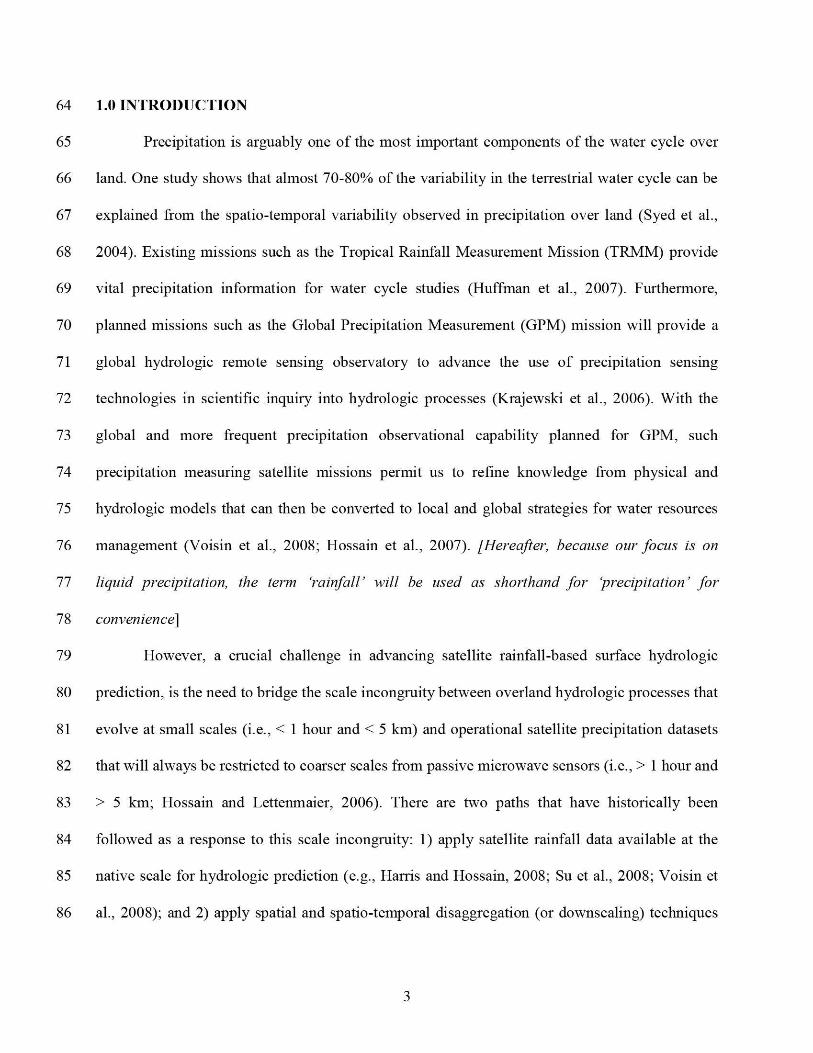
152 boxes). Figure 1 provides a conceptual rendition of this idea of `transfer' of uncertainty based on
153 the concept of spatial interpolation (taken from Ling and Hossain, 2009).
154 This paper analyzes the open issues for developing an appropriate uncertainty transfer
155 scheme that can routinely estimate various uncertainty metrics across the globe by leveraging a
6
156 combination of spatially-dense GV data and temporally sparse surrogate (or proxy) GV data
157 from sources such as the TRMM-like PR sensor anticipated during the GPM era. The TRMM
158 Multi-satellite Precipitation Analysis (TMPA) products 31342RT and 31341RT (Huffman et al.,
159 2007) over the US spanning a record of 6 years are used as a representative example of satellite
160 rainfall. The paper presents a probabilistic analysis of sampling offered by the existing
161 constellation of precipitation-relevant satellite PMW sensors in order to understand the current
162 and expected spatial coverage during the GPM era. A commonly used spatial interpolation
163 technique (kriging), that leverages the spatial correlation of rainfall estimation uncertainty, is
164 then investigated for its effectiveness. This effectiveness is cast in the context of the expected
165 sparseness in GV data expected from TRMM and GPM missions. Finally, important issues
166 needing closure are summarized on the basis of our investigation of transfer of satellite rainfall
167 uncertainty from GV to non-GV regions. To avoid confusion among readers, hereafter, the terms
168 `uncertainty' or `uncertainty metric' will be used to define the quality indices of the satellite
169 rainfall estimate derived at GV locations (such as bias, root mean squared error, probability of
170 detection). The terms `error' or `transfer error' will be used specifically to define the quality of
171 the transfer (spatial interpolation) process of uncertainty metrics at non-GV locations.
172173 2.0 SPATIAL CORRELATION OF SATELLITE RAINFALL UNCERTAINTY
174 The very first requirement for an effective transfer (spatial interpolation) scheme is the
175 presence of a quantifiable spatial structure (or spatial correlation) in the variable being
176 transferred. Therefore, we first investigated the presence of spatial correlation of satellite rainfall
177 uncertainty. First, in order to minimize the error of the GV rainfall data, we used the National
178 Center for Environmental Prediction's (NCEP) 4 km Stage IV NEXRAD rainfall data that is
179 adjusted to precipitation gages and conveniently available as a quality-controlled data mosaic
7
180 over the U.S. (Lin and Mitchell, 2005; Fulton et al., 1998). TMPA's near real-time satellite
181 rainfall data-products from PMW-calibrated Infrared (IR) and merged PMW-IR estimates
182 (labeled 31341 RT and 31342RT, respectively; Huffman et al., 2007) were used as the satellite
183 rainfall data. The data for GV and satellite rainfall data spanned 6 years from 2002 to 2007. The
184 NEXRAD Stage IV GV rainfall data were first remapped to 0.25° 3-hourly resolution for
185 consistency with the native scale of the satellite rainfall products. 31341RT data were also
186 remapped at the 3-hourly time scale. After a thorough quality assessment and quality control
187 (QA/QC), the datasets were organized by season and various regions for the years 2002-2007.
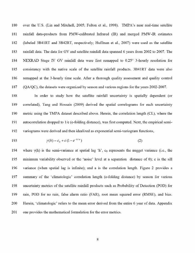
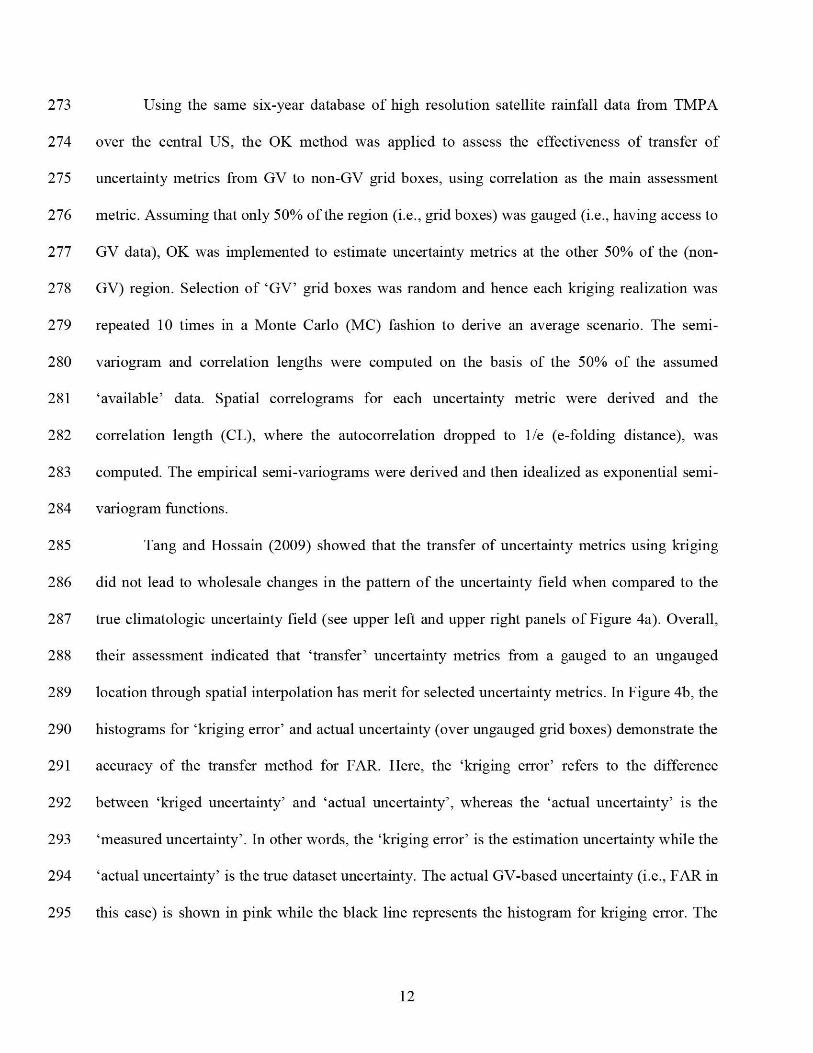
188 In order to study how the satellite rainfall uncertainty is spatially dependent (or
189 correlated), Tang and Hossain (2009) derived the spatial correlograms for each uncertainty
190 metric using the TMPA dataset described above. Herein, the correlation length (CL), where the
191 autocorrelation dropped to 1/e (e-folding distance), was first computed. Next, the empirical semi-
192 variograms were derived and then idealized as exponential semi-variogram functions,
193 7(h) = cp + c (1— e -"') (2)
194 where y(h) is the semi-variance at spatial lag `h', co represents the nugget variance (i.e., the
195 minimum variability observed or the `noise' level at a separation distance of 0); c is the sill
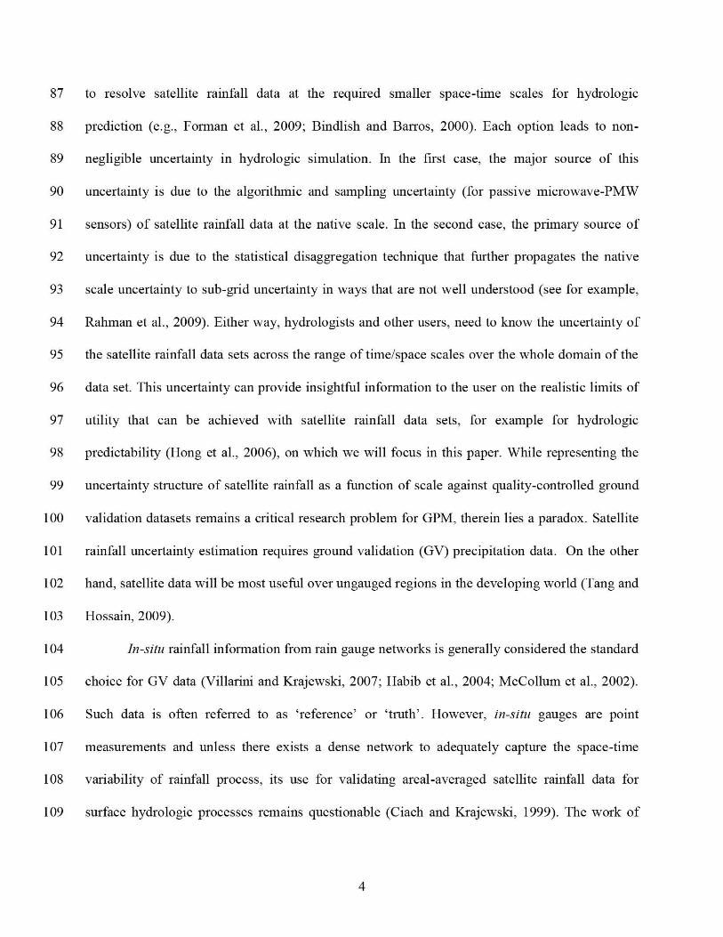
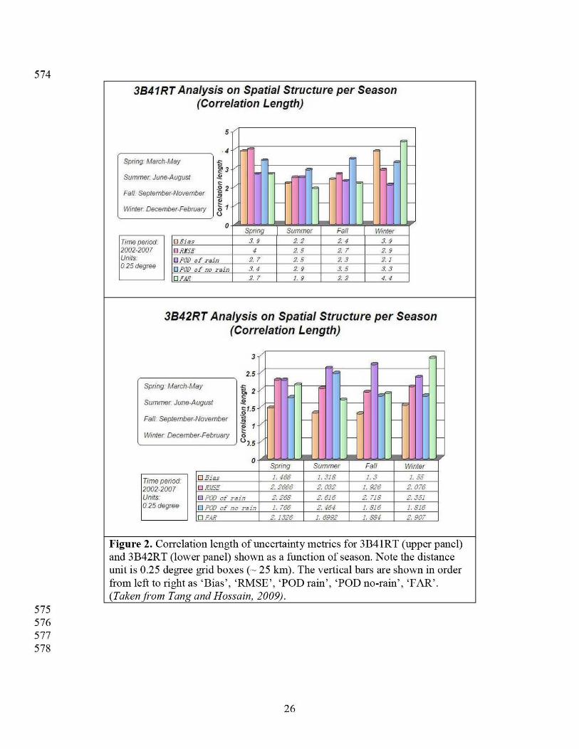
196 variance (when spatial lag is infinite); and a is the correlation length. Figure 2 provides a
197 summary of the `climatologic' correlation length (e-folding distance) by season for various
198 uncertainty metrics of the satellite rainfall products such as Probability of Detection (POD) for
199 rain, POD for no rain, false alarm ratio (FAR), root mean squared error (RMSE), and bias.
200 Herein, `climatologic' refers to the mean error derived from the entire 6 year of data. Appendix
201 one provides the mathematical formulation for the error metrics.
8
202 Figure 2 clearly demonstrates that, at the climatologic (long-term) time scale, satellite
203 rainfall uncertainty can have distinct spatial organization that can be leveraged for spatial
204 interpolation. The correlation lengths for a given uncertainty metric as a function of season
205 appear to be at least 3-5 (0.25°) TMPA grid boxes long. As a rule of thumb, this indicates that
206 the transfer of error from sampled locations may be effective up to 4 grid boxes (— 100 km)
207 away. Another interesting feature that is revealed in this figure is the significantly higher
208 correlation lengths (and spatial organization) observed for 31341RT than 31342RT. This can be
209 traced to the sources of the specific satellite estimates: 31341RT is uniformly computed using a
210 calibration of infrared (IR) brightness temperatures to a combined PMW estimate. The statistics
211 of the uncertainty are spatially very homogenous since they originate from a single probability
212 distribution at regional scales. On the other hand, 31342RT uses a variety of PMW rainfall
213 estimates with gaps filled during a 3-hour sampling period with the 31341RT estimate `as is'.
214 This fill-in causes the 31342RT data to draw on two different probability distributions in space
215 for uncertainty statistics (IR and PMW); the increased spatial heterogeneity in the uncertainty
216 structure leads to shorter correlation length. This analysis shows that any uncertainty transfer
217 scheme should benefit from improvements in the 31342RT product to make it statistically more
218 homogenous in space.
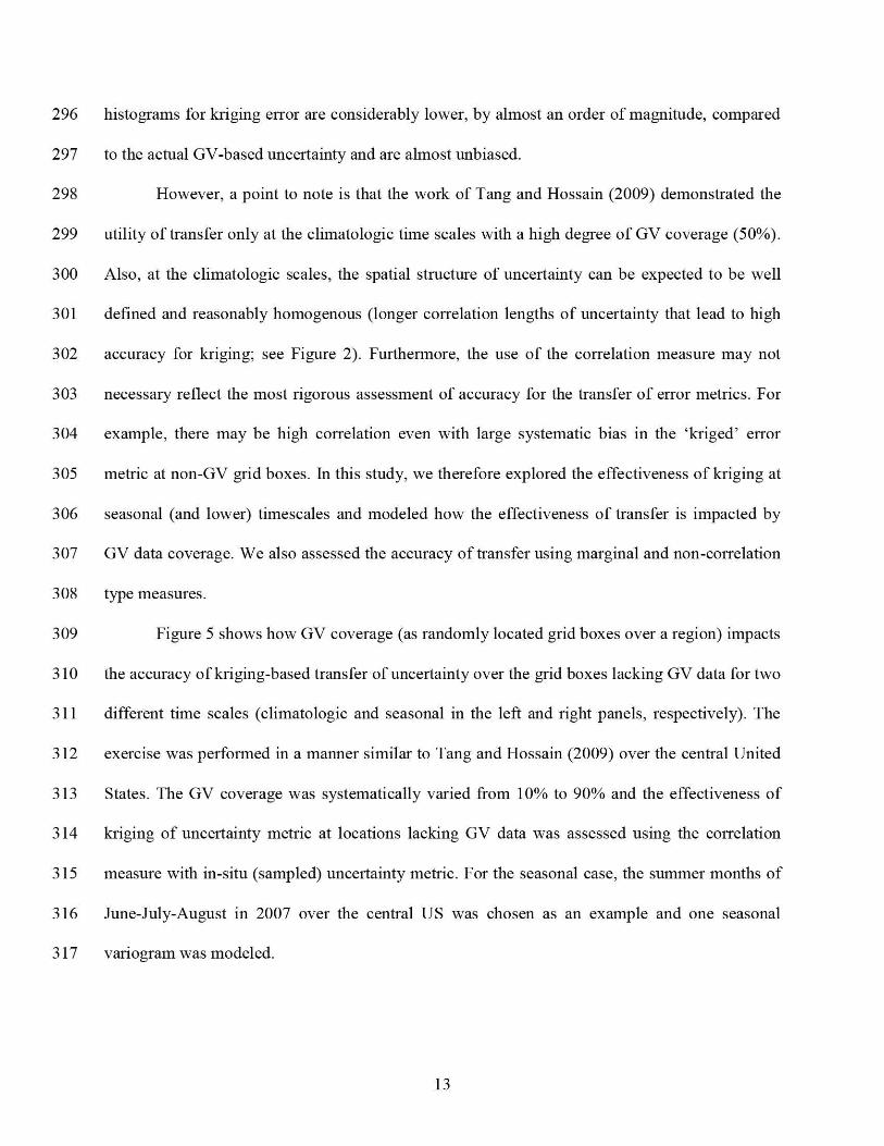
219220 3.0 SPATIAL COVERAGE OFFERED BY CURRENT CONSTELLATION OF PMW221 SENSORS222223 Having observed a distinct spatial organization of uncertainty, we also need to understand
224 the space/time dimension that is implicit in the concept of real-time uncertainty `transfer' over
225 non-GV regions. The space dimension pertains to the regions with spatially sparse GV data due
226 to inadequate in-situ gauge data (such as that shown in Figure 1), which are, of course, recorded
9
227 at fixed positions. The time dimension pertains to the temporally sparse case of using the most
228 accurate rainfall source currently available from space, such as the orbiting TRMM PR as
229 'proxy'-GV data, over regions where there is no ground-based GV data. Depending on how we
230 define GV data, there can be several types of GV `voids' where uncertainty information will be
231 need to be estimated for GPM. For example, if we rely on the `conventional' ground source for
232 GV data, voids will be represented by large and stationary regions having little or no
233 instrumentation. On the other hand, if a `proxy' for GV is defined from orbiting sensors, such as
234 the TRMM PR, or even a highly accurate PMW sensor, then voids will be numerous grid boxes
235 dynamically changing in location with each satellite orbit.
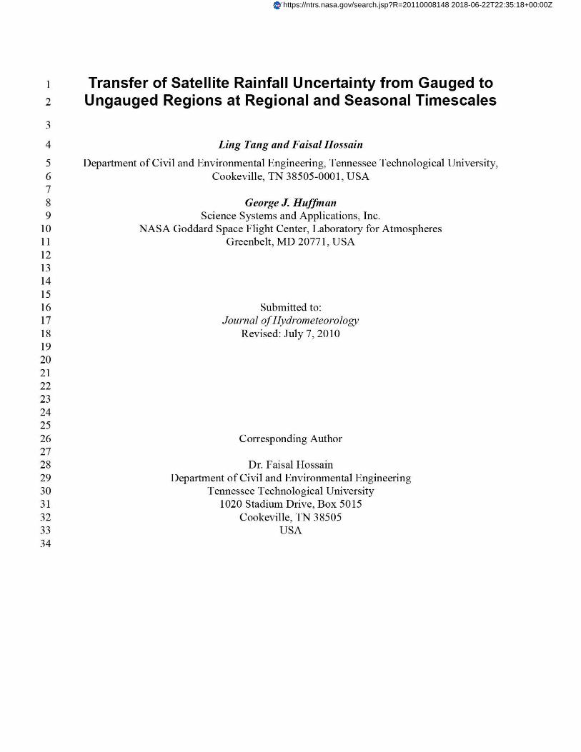
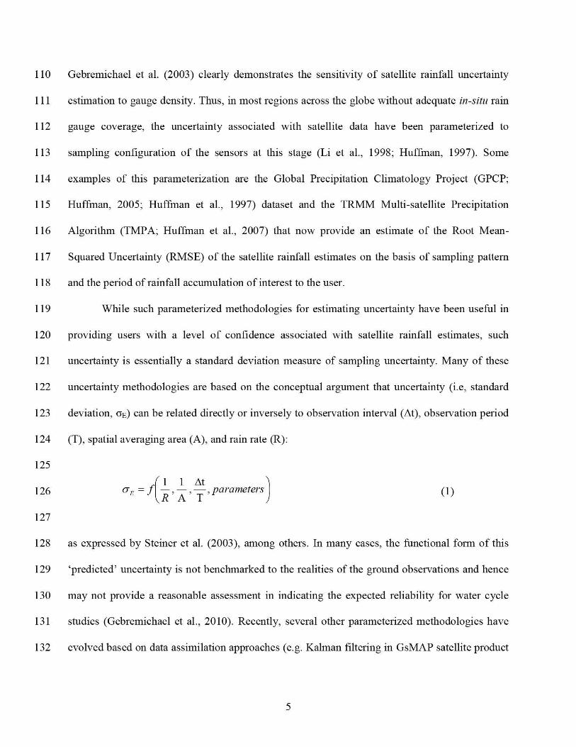
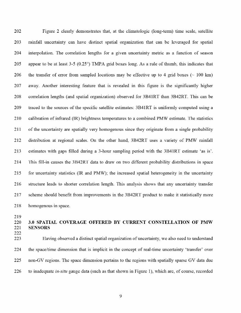
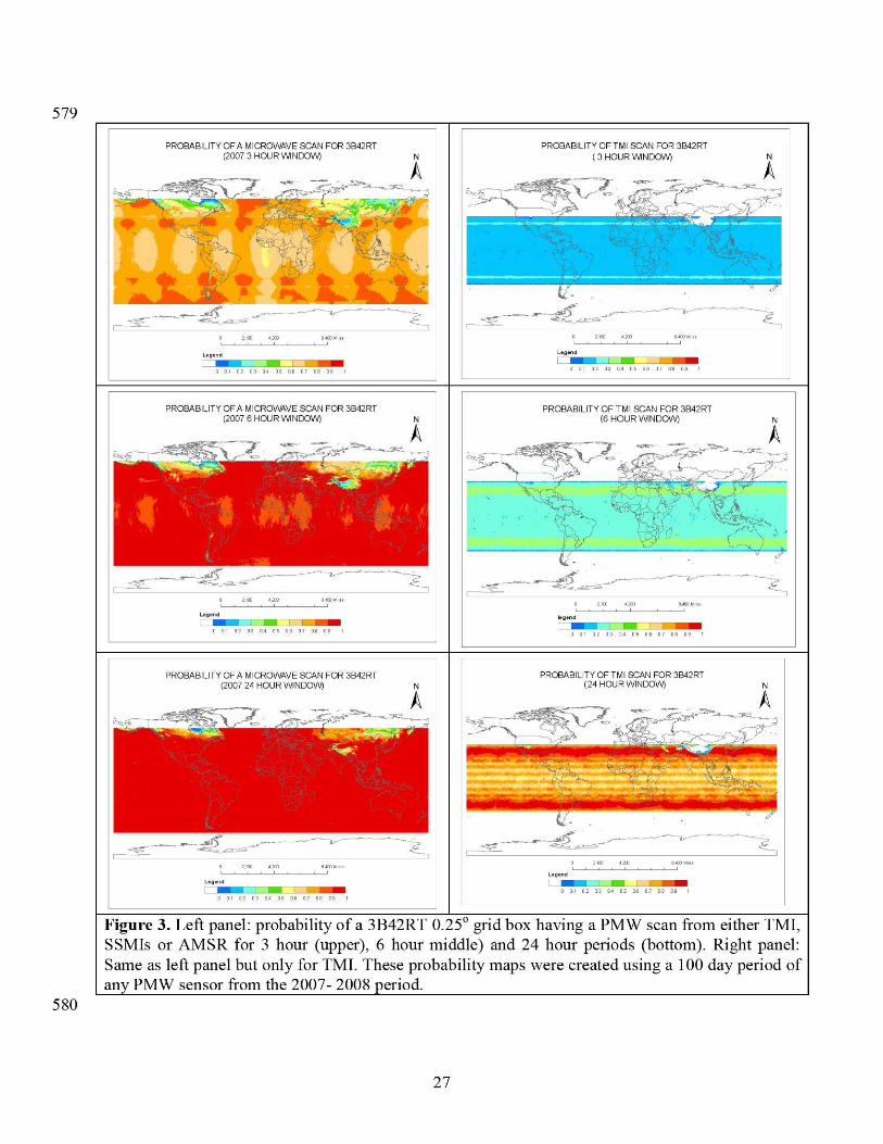
236 The left panel of Figure 3 shows the probability of a 31342RT grid box (0.25) having a
237 conical-scanning PMW overpass (comprising either TMI, SSMI or AMSR) in 3, 6 and 24 hour
238 windows. On the right panels of Figure 3, the probability of a 31342RT grid box having a TRMM
239 Microwave Imager (TMI) scan is shown. These probability maps were created using a 100 day
240 period of any PMW sensor) from the 2007- 2008 period. It is clear from the maps that the spatio-
241 temporal dynamics of the location of PMW scans is strongly sensitive to the accumulation
242 periods of hydrologic relevance and one that must be investigated carefully in order to identify
243 how an uncertainty transfer scheme may work using proxy-GV data.
244 At time scales of 3-6 hours, there are vast regions lacking conventional surface GV data
245 in the tropics of Africa, Asia and South America where the probability of having a PMW scan is
246 less than 50% (Figure 3). This makes the estimation of uncertainty through transfer from GV
247 regions at these locations more important for hydrologic applications. While GPM may improve
248 the coverage of PMW scans, such large voids with a low probability for a PMW scan will still
249 remain over these regions due the continued dependence on polar-orbiting sensors. Since gauge-
10
250 based GV is sparse for these tropical regions at hydrologic scales, proxy GV data from space-
251 borne sensors (such as that expected from the GPM Dual Frequency Precipitation Radar) may be
252 one of the few ways to explore if `transfer' of uncertainty is realistic. For the higher latitude land
253 regions (which comprise mostly the industrialized world with reasonably gauged fixed-location
254 GV instrumentation), the uncertainty could be transferred from the stationary GV regions. The
255 right panels of Figure 3 also show that the probability of having a TMI scan also happens to be
256 lowest (0.1-0.2 in 3 hours) over the tropical regions. However, over a 24 hour time period there
257 is considerably higher probability of having such a scan (--0.7-0.8). This implies that the
258 practicable timescale for transferring uncertainty metrics over the tropics from a sun-
259 asynchronous PMW sensor is at least 24 hours.
260
261 4.0 TRANSFER OF UNCERTAINTY BY SPATIAL INTERPOLATION
262 Tang and Hossain (2009) recently showed that most uncertainty metrics (such as bias and
263 POD) are amenable to `transfer' from gauged to ungauged locations using spatial interpolation at
264 climatologic (six-year average) timescales. The method of ordinary kriging (OK) was used for
265 testing the `transfer' of uncertainty metrics. OK is the most common (and one of the simplest)
266 spatial interpolation estimator used to find the best linear unbiased estimate of a second-order
267 stationary random field with an unknown constant mean as follows:
268 Z(xo) _ Aaz( xi) (3)
269 where Z(xo )= kriging estimate at location xo; Z(x i) = sampled value at location x i; ki =
270 weighting factor for Z(x i) (summing to one over all 1), and n is the number of sampled (known)
271 locations. Kriging methods have already been used for spatial interpolation of precipitation from
272 point gauge data with considerable success (see for example, Seo et al., 1990; Krajewski, 1987).
11
273 Using the same six-year database of high resolution satellite rainfall data from TMPA
274 over the central US, the OK method was applied to assess the effectiveness of transfer of
275 uncertainty metrics from GV to non-GV grid boxes, using correlation as the main assessment
276 metric. Assuming that only 50% of the region (i.e., grid boxes) was gauged (i.e., having access to
277 GV data), OK was implemented to estimate uncertainty metrics at the other 50% of the (non-
278 GV) region. Selection of `GV' grid boxes was random and hence each kriging realization was
279 repeated 10 times in a Monte Carlo (MC) fashion to derive an average scenario. The semi-
280 variogram and correlation lengths were computed on the basis of the 50% of the assumed
281 `available' data. Spatial correlograms for each uncertainty metric were derived and the
282 correlation length (CL), where the autocorrelation dropped to 1/e (e-folding distance), was
283 computed. The empirical semi-variograms were derived and then idealized as exponential semi-
284 variogram functions.
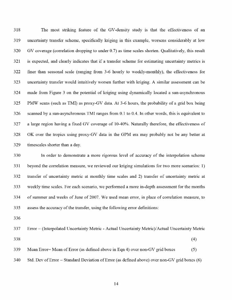
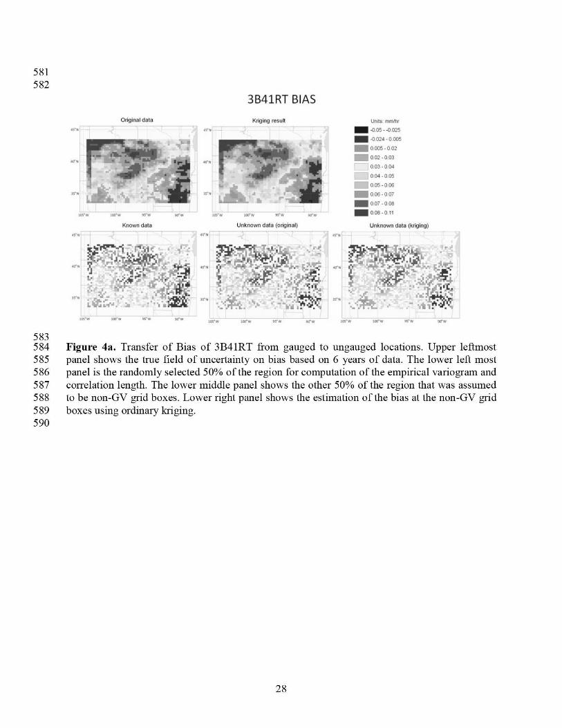
285 Tang and Hossain (2009) showed that the transfer of uncertainty metrics using kriging
286 did not lead to wholesale changes in the pattern of the uncertainty field when compared to the
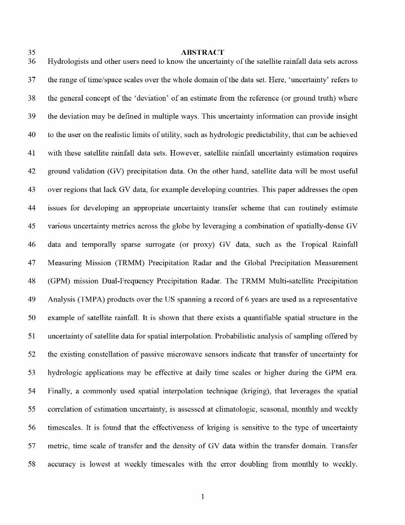
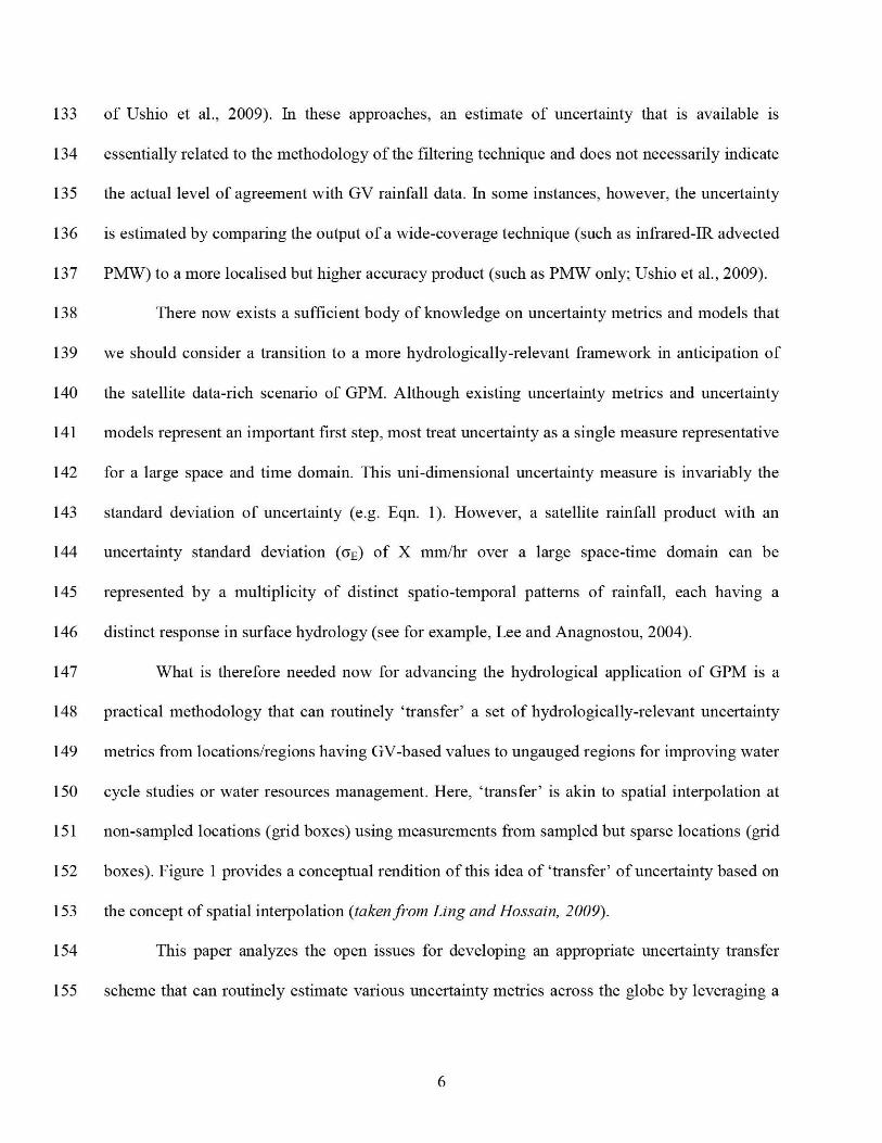
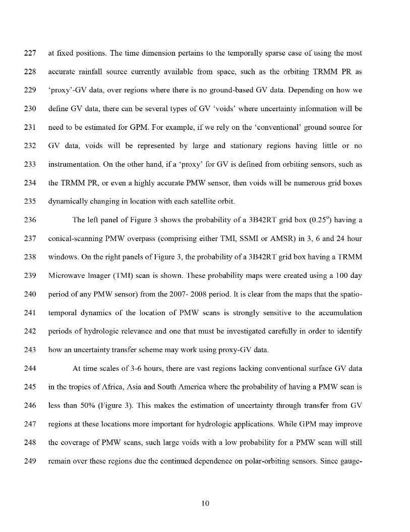
287 true climatologic uncertainty field (see upper left and upper right panels of Figure 4a). Overall,
288 their assessment indicated that `transfer' uncertainty metrics from a gauged to an ungauged
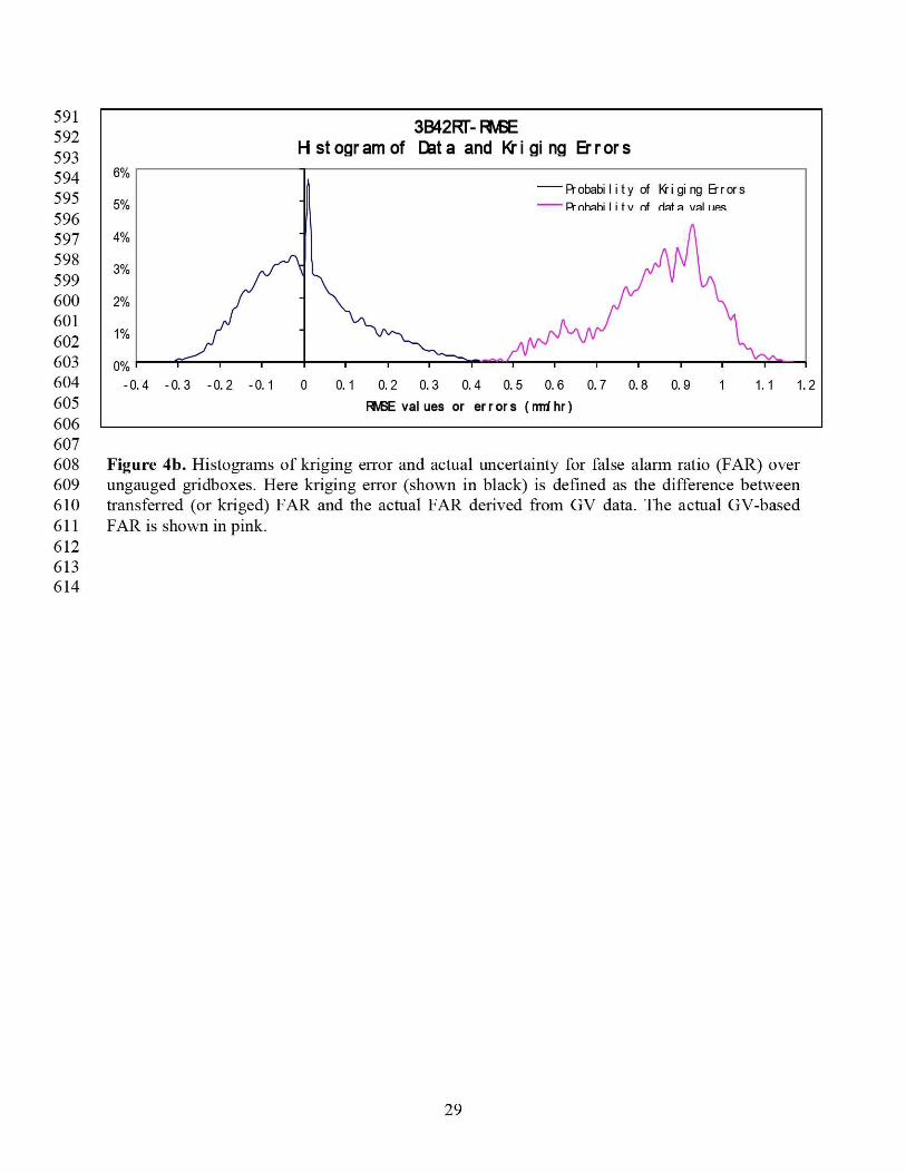
289 location through spatial interpolation has merit for selected uncertainty metrics. In Figure 4b, the
290 histograms for `kriging error' and actual uncertainty (over ungauged grid boxes) demonstrate the
291 accuracy of the transfer method for FAR. Here, the `kriging error' refers to the difference
292 between `kriged uncertainty' and `actual uncertainty', whereas the `actual uncertainty' is the
293 `measured uncertainty'. In other words, the `kriging error' is the estimation uncertainty while the
294 `actual uncertainty' is the true dataset uncertainty. The actual GV-based uncertainty (i.e., FAR in
295 this case) is shown in pink while the black line represents the histogram for kriging error. The
12
296 histograms for kriging error are considerably lower, by almost an order of magnitude, compared
297 to the actual GV-based uncertainty and are almost unbiased.
298 However, a point to note is that the work of Tang and Hossain (2009) demonstrated the
299 utility of transfer only at the climatologic time scales with a high degree of GV coverage (50%).
300 Also, at the climatologic scales, the spatial stricture of uncertainty can be expected to be well
301 defined and reasonably homogenous (longer correlation lengths of uncertainty that lead to high
302 accuracy for kriging; see Figure 2). Furthermore, the use of the correlation measure may not
303 necessary reflect the most rigorous assessment of accuracy for the transfer of error metrics. For
304 example, there may be high correlation even with large systematic bias in the `kriged' error
305 metric at non-GV grid boxes. In this study, we therefore explored the effectiveness of kriging at
306 seasonal (and lower) timescales and modeled how the effectiveness of transfer is impacted by
307 GV data coverage. We also assessed the accuracy of transfer using marginal and non-correlation
308 type measures.
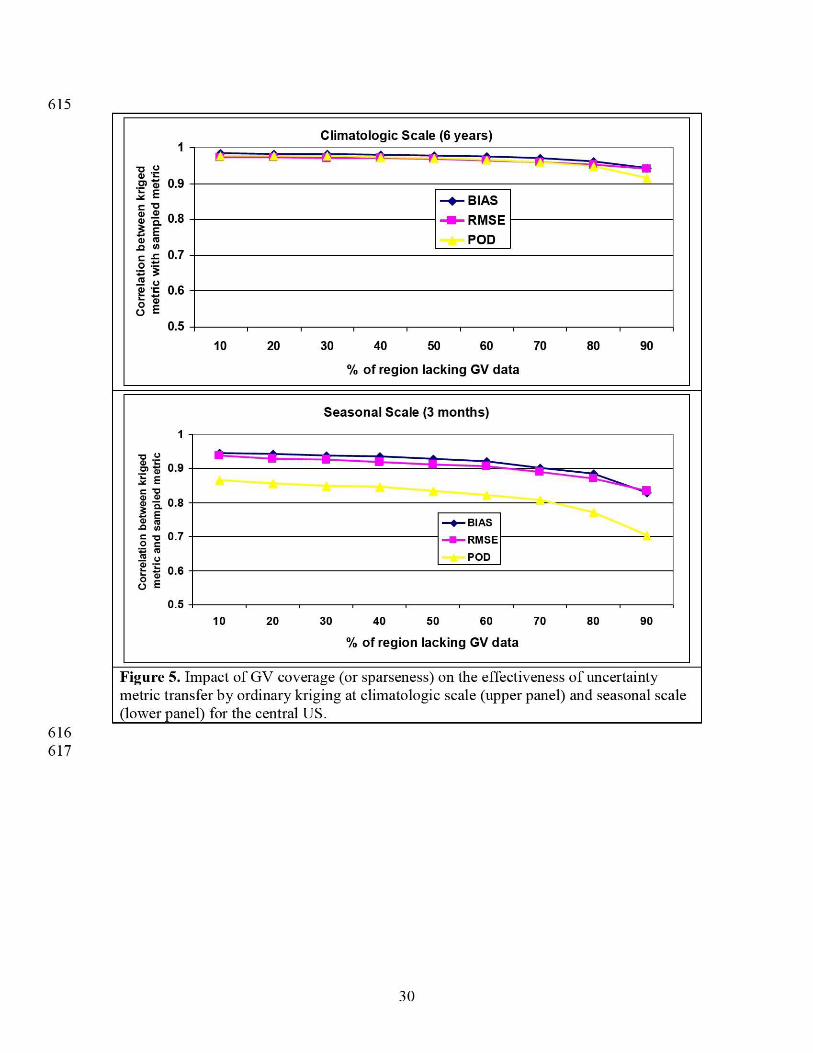
309 Figure 5 shows how GV coverage (as randomly located grid boxes over a region) impacts
310 the accuracy of kriging-based transfer of uncertainty over the grid boxes lacking GV data for two
311 different time scales (climatologic and seasonal in the left and right panels, respectively). The
312 exercise was performed in a manner similar to Tang and Hossain (2009) over the central United
313 States. The GV coverage was systematically varied from 10% to 90% and the effectiveness of
314 kriging of uncertainty metric at locations lacking GV data was assessed using the correlation
315 measure with in-situ (sampled) uncertainty metric. For the seasonal case, the summer months of
316 June-July-August in 2007 over the central US was chosen as an example and one seasonal
317 variogram was modeled.
13
318 The most striking feature of the GV-density study is that the effectiveness of an
319 uncertainty transfer scheme, specifically kriging in this example, worsens considerably at low
320 GV coverage (correlation dropping to under 0.7) as time scales shorten. Qualitatively, this result
321 is expected, and clearly indicates that if a transfer scheme for estimating uncertainty metrics is
322 finer than seasonal scale (ranging from 3-6 hourly to weekly-monthly), the effectiveness for
323 uncertainty transfer would intuitively worsen further with kriging. A similar assessment can be
324 made from Figure 3 on the potential of kriging using dynamically located a sun-asynchronous
325 PMW scans (such as TMI) as proxy-GV data. At 3-6 hours, the probability of a grid box being
326 scanned by a sun-asynchronous TMI ranges from 0.1 to 0.4. In other words, this is equivalent to
327 a large region having a fixed GV coverage of 10-40%. Naturally therefore, the effectiveness of
328 OK over the tropics using proxy-GV data in the GPM era may probably not be any better at
329 timescales shorter than a day.
330 In order to demonstrate a more rigorous level of accuracy of the interpolation scheme
331 beyond the correlation measure, we reviewed our kriging simulations for two more scenarios: 1)
332 transfer of uncertainty metric at monthly time scales and 2) transfer of uncertainty metric at
333 weekly time scales. For each scenario, we performed a more in-depth assessment for the months
334 of summer and weeks of June of 2007. We used mean error, in place of correlation measure, to
335 assess the accuracy of the transfer, using the following error definitions:
336
337 Error = (Interpolated Uncertainty Metric - Actual Uncertainty Metric)/Actual Uncertainty Metric
338 (4)
339 Mean Error= Mean of Error (as defined above in Eqn 4) over non-GV grid boxes (5)
340 Std. Dev of Error = Standard Deviation of Error (as defined above) over non-GV grid boxes (6)
14
341 Tables la and lb summarize the assessment of OK method using mean relative error
342 (Eqn 5) as the main assessment metric for transfer of uncertainty metrics — BIAS, RMSE, POD
343 and FAR. For each uncertainty metric both mean and standard deviation of error of transfer is
344 shown as measures of accuracy and precision, respectively. It is observed that, unlike correlation
345 measure, the mean and standard deviation of error reveal a somewhat different picture on the
346 utility of OK method. The error metric BIAS has the lowest accuracy ranging from 50% error (at
347 10% missing GV gridboxes) to 100% error (at 90% missing GV gridboxes) for monthly time
348 scale. For weekly timescale, the mean error ranges from 80% (at 10% missing GV grid boxes) to
349 120% (at 90% missing GV grid boxes). On the other hand, POD, followed by RMSE and FAR,
350 have the highest accuracy for transfer of error metrics at both timescales according the mean
351 relative error measure. As expected, the precision of the kriging based transfer scheme degrades
352 at shorter timescales. At very low GV coverage (<20%) the standard deviation of transfer error is
353 high (>100%), indicating poor performance of the OK method regardless of the timescale at
354 which the uncertainty metrics are transferred.
355
356 5.0 CONCLUSION: THE CURRENT OPEN ISSUES ON UNCERTAINTY TRANSFER
357 In light of the impact of GV coverage and the timescale on effectiveness of uncertainty
358 transfer, we now need to consider the following: 1) explore other techniques for transfer that are
359 more sophisticated than ordinary kriging; and 2) understand how we can leverage the
360 methodological error estimate that is routinely available from uncertainty models such as
361 Huffman (1997) and Kalman filtering techniques that many satellite rainfall data algorithms use
362 (such as, Ushio et al. 2009). In our interpolation method, the spatial structure of rainfall has not
363 been used alongside that of estimation uncertainty. Because the two (rainfall and its estimation
15
364 uncertainty) are related, it may be worthwhile to pursue co-kriging type conditional interpolation
365 schemes that leverage existing information on the satellite rainfall distribution as an extra
366 constraint.
367 Also, for spatial interpolation methods, we should keep in mind that traditional
368 geostatistical tools are pattern filling methods based on the spatial correlation exhibited by two
369 points in space separated by a lag h. The variogram computed using this two-point geostatistical
370 approach may simplify the spatial patterns manifested by the complex precipitation systems and
371 surface emissivities that dictate the accuracy of satellite rainfall products at hydrologic time
372 scales over land. For the case of spatial interpolation of ground water contamination, it has
373 recently been demonstrated that the use of a highly non-linear pattern learning technique in the
374 form of an artificial neural network (ANN) can yield significantly superior results under the
375 same set of constraints when compared to ordinary kriging method (Chowdhury et al., 2009).
376 Thus, the use of non-linear mapping techniques are worth an investigation.
377 Another aspect to keep in mind is the nature of use of each uncertainty metrics. Different
378 users will have naturally different needs. Hydrologist users engaged in flash flood or monsoonal
379 flood forecasting will probably be more interested in the PODS (to understand the accuracy in
380 estimating peak flow), FAR (to minimize false alarms in flood warnings), and BIAS (to
381 minimize under/over estimation in river stage) for each grid box (see Harris and Hossain, 2008
382 and Hossain and Anagnostou, 2004). Hydrologists engaged in continuous simulation based on
383 soil moisture accounting for drought monitoring and water management would probably focus
384 more on PODNORAIN (to minimize uncertainty in underestimating the soil wetness and
385 evapotranspiration) for each grid box. On the other hand, crop yield and famine forecasters
386 would like to focus more on the seasonal bias over a large agricultural zone during the growing
16
387 season as the important indicator of reliability of a satellite rainfall product (personal
388 communication with Dr. Chris Funk of University of California Santa Barbara).
389 In summary, developing an uncertainty transfer scheme that is amenable to operational
390 implementation for estimation of uncertainty metrics for satellite rainfall data over regions
391 lacking surface GV data is a necessary requirement for current and future satellite precipitation
392 missions to advance their hydrologic potential. Hydrologist users around the world need to have
393 a clear understanding of the pros and cons of applying satellite rainfall data for terrestrial
394 hydrologic applications at a given scale if the benefit of these missions is to be maximized. One
395 way of facilitating the understanding is through the routine provision of various measures of
396 uncertainty that are of hydrologic relevance. If this uncertainty information is provided alongside
397 the global and more frequent precipitation observational capability planned in GPM, it will
398 permit us to refine knowledge from physical and hydrologic models that can then be converted to
399 local and global strategies for water resources management. Work is currently undergoing to
400 address some of the open issues discussed above and we hope to report them in the near future.
401
402 Acknowledgement: The first author (Tang) was supported by the NASA Earth System Science
403 Fellowship (2008-2011). The second author (Hossain) was supported by the NASA New
404 Investigator Program Award (NNX08AR32G).
405
406
407
17
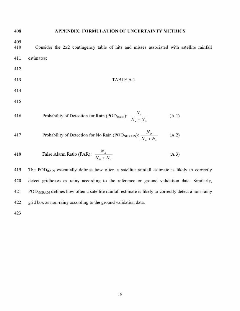
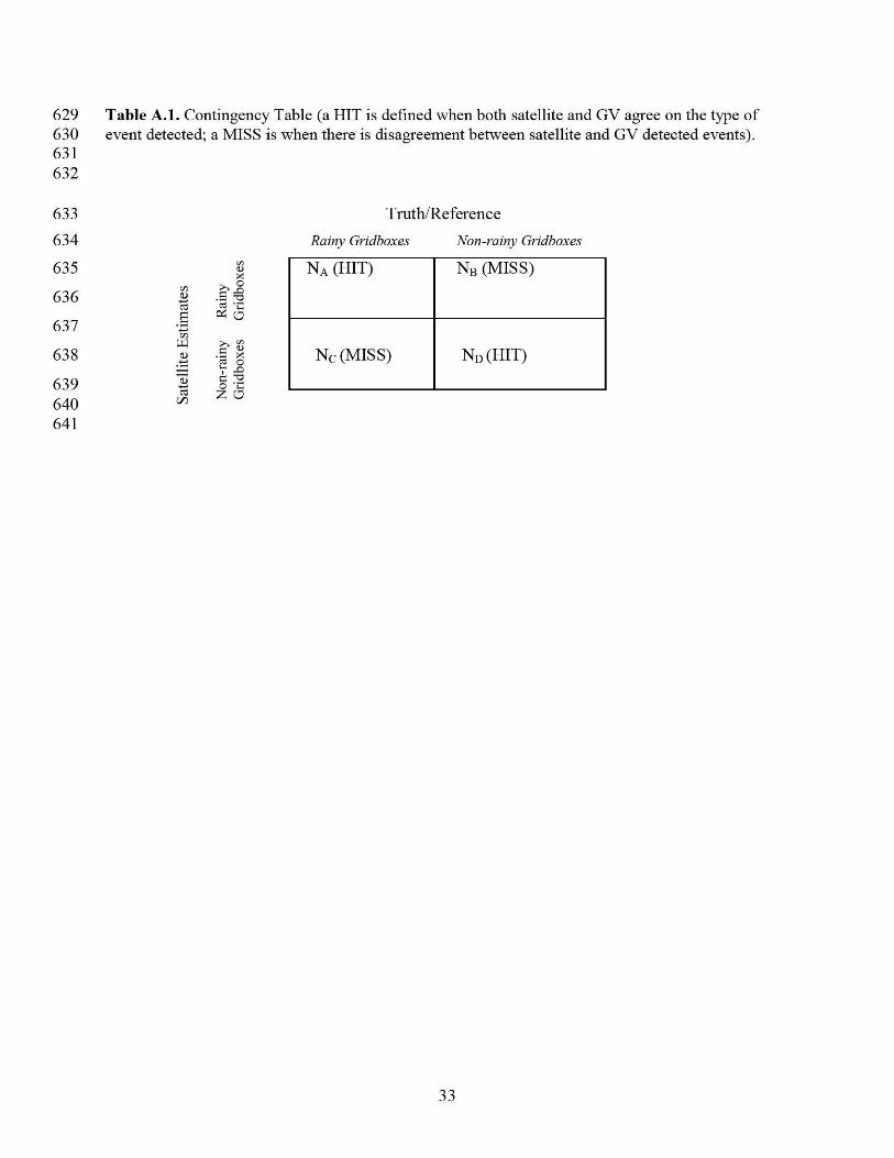
408 APPENDIX: FORMULATION OF UNCERTAINTY METRIC'S
409410 Consider the 2x2 contingency table of hits and misses associated with satellite rainfall
411 estimates:
412
413
TABLE A.1
414
415
416 Probability of Detection for Rain (PODS): NA
(A.1)N, +N,
417 Probability of Detection for No Rain (PODNORAIN):N
N + N(A 2)
D C
418 False Alarm Ratio (FAR): NB (A.3)NB + NA
419 The PODRAIN essentially defines how often a satellite rainfall estimate is likely to correctly
420 detect gridboxes as rainy according to the reference or ground validation data. Similarly,
421 PODNOxaIN defines how often a satellite rainfall estimate is likely to correctly detect a non-rainy
422 grid box as non-rainy according to the ground validation data.
423
18
424 REFERENCES
425 Anagnostou, E.N. 2004: Overview of overland satellite rainfall estimation for hydro-
426 meteorological applications. Surveys in Geophysics, 25(5-6), pp. 511-537.
427 Bindlish, R., A.P. Barros. 2000: Disaggregation of rainfall for one-way coupling of atmospheric
428 and hydrological models in regions of complex terrain. Global and Planetary Change, 25,
429 pp. 111-132.
430 Ciach, G.J. and W.F. Krajewski. 1999: Radar-rain gauge comparisons under observational
431 uncertainties, Journal of Applied AVleteor•ology, 38(10),519-1525.
432 Chowdhury, M., A. Alouani, and F. Hossain. 2009: How much does inclusion of Non-linearity
433 affect the Spatial Mapping of Complex Patterns of Groundwater Contamination? Non-Linear
434 Processes in Geophysics, 16, 313-317
435 Forman, B., E. Vivom, and S. Margulis. 2008: Evaluation of Ensemble-based Distributed
436 Hydrologic Model Response with Disaggregated Precipitation Products, Water Resources
437 Research, 44, W 12409, dol:10.1029/2008WR006827.
438 Fulton, R.A., J.P. Breidenbach, D.-J. Seo, D.A. Miller, and T. O'Bannon, T. 1998: The WSR-
439 88D rainfall algorithm. Weather and Forecasting, 13(2), 377-395.
440 Gebremichael, M., W.F. Krajewski, M. Morrissey, D. Langerud, G. J. Huffman and R. Adler.
441 2003: Uncertainty uncertainty analysis of GPCP monthly rainfall products: A data based
442 simulation study. Journal ofApplied tvleteorology, 42(12), 1837-1848.
443 Gebremichael, M., E.N. Anagnostou and M. Bitew. (2010) Critical Steps for Continuing
444 Advancement of Satellite Rainfall Applications for Surface Hydrology in the Nile River
445 Basin, Journal of the American Water Resources Association, (doi: 10.1111/j.1752-
446 1688.2010.00428.x).
19
447 Habib, E., G.J. Ciach, and W.F. Krajewski. 2004: A method for filtering out rain gauge
448 representativeness uncertainty from the verification distributions of radar and raingauge
449 rainfall. Advances in Water Resources, 27(10), 967-980.
450 Harris, A. and F. Hossain. 2008: Investigating Optimal Configuration of Conceptual Hydrologic
451
Models for Satellite Rainfall-based Flood Prediction for a Small Watershed, IEEE
452
Geosciences and Remote Sensing Letters, 5(3), July.
453
Hossain, F. and G.J. Huffman. 2008: Investigating uncertainty metrics for satellite rainfall at
454
hydrologically relevant Scales, Journal of Hydrometeorology, 9(3), 563-575.
455
Hossain, F., N. Katiyar, A. Wolf, and Y. Hong. 2007: The Emerging role of satellite rainfall data
456
in improving the hydro-political situation of flood monitoring in the under-developed regions
457 of the world, Natural Hazards (Special Issue). INVITED PAPER, 43,199-210.
458 Hossain, F., D.P. Lettenmaier. 2006: Flood prediction in the future: recognizing hydrologic
459 issues in anticipation of the global precipitation measurement mission - Opinion Paper.
460 Water Resources Research. 44 (doi: 10.1029/2006WR005202)
461 Hossain, F., and E.N. Anagnostou. 2004: Assessment of current passive microwave and infra-red
462 based satellite rainfall remote sensing for flood prediction, Journal of Geophysical Research.
463 109(D7), April, D07102. (doi 10. 1 029/2003JD003986).
464 Hong Y., K. Hsu, H. Moradkhani, and S. Sorooshian 2006: Uncertainty Quantification of
465
Satellite Precipitation Estimation and Monte Carlo Assessment of the Uncertainty
466
Propagation into Hydrologic Response, Water Resources Research, 42, W08421
467
(dOi:10.1029/2005WR004398).
20
468 Hou, A., G.S. Jackson, C. Kummerow, C., and C.M. Shepherd. 2008: Global Precipitation
469 Measurement, In Precipitation: Advances in Measurement, Estimation, and Prediction, (eds)
470 Silas Michaelides, pp. 1-39, Springer Publishers.
471 Huffman, G.J., R.F. Adler, D.T. Bolvin, G. Gu, E.J. Nelkin, K.P. Bowman, Y. Hong, E.F.
472 Stocker, and D.B. Wolff. 2007: The TRMM multi-satellite precipitation analysis: Quasi-
473 global, multi-year, combined sensor precipitation estimates at fine scales, Journal of
474 Hydroweteorology, 8,28-55.
475 Huffman, G.J. 2005: Hydrological applications of remote sensing: Atmospheric states and fluxes
476 — precipitation (from satellites) (active and passive techniques). In Encyclopedia for
477 Hydrologic Sciences, M.G. Anderson and J. McDonnel (Eds) (ISBN: 978-0-471-49103-3).
478 Huffman, G.J., R.F. Adler, M.M. Morrissey. and others. 2001: Global precipitation at one-degree
479 daily resolution from multi satellite observations. Journal of Hydrometeor •ology, 2,36-50.
480 Huffman, G.J. 1997: Estimates of root mean square random uncertainty for finite samples of
481 estimated precipitation, Journal of Applied Meteorology, 36, 1191-1201.
482 Joyce, R.L., J.E. Janowiak, P.A. Arkin, and P. Xie. 2004: CMORPH: A method that produces
483 global precipitation estimates from passive microwave and infrared data at high spatial and
484 temporal resolution. Journal of Hvdrometeorology, 5, 487-503.
485 Krajewski, W. F., et al. 2006: A remote sensing observatory for hydrologic sciences: A genesis
486 for scaling to continental hydrology, Water Resources Research, 42, W07301,
487 doi:10.1029/2005WR004435.
488 Krajewski, W. 1987: Cokriging Radar Rainfall and Rain Gage Data, Journal of Geophysical.
489 Research, 92(D8), 9571-9580.
21
490 Lee, K.H and E.N. Anagnostou. 2004: Investigation of the nonlinear hydrologic response to
491 precipitation forcing in physically based land surface modeling. Canadian Journal of Remote
492 Sensing, 30, 706-716.
493 Li, Q., R. Ferraro, and N.C. Grody. 1998: Detailed analysis of the uncertainty associated with
494 rainfall retrieved NOAA/NESDIS SSM/I rainfall algorithm: Part I, tropical oceanic rainfall.
495 Journal of Applied Meteorology, 39,680-685.
496 Lin, Y., and K. Mitchell. 2005: The NCEP Stage II/IV hourly precipitation analyses: 199
497 development and applications. 19th ANIS Conference on Hydrology.
498 McCollum, J.R., W.F. Krajewski, R.R. Ferraro, and M.B. Ba. 2002: Evaluation of biases of
499 satellite rainfall estimation algorithms over the continental United States. Journal of Applied
500 Meteorology, 41(11), 1065-1080.
501 Rahman, S., A.C. Bagtzoglou, F. Hossain, L. Tang, L.Yarbrough, G. Easson, G. 2009:
502 Investigating Spatial Downscaling of Satellite Rainfall Data for Flood Prediction, Journal of
503 Hydronneteor•ology, doi:10.1175/2009JHM 1072.1
504 Seo, D.J., W. Krajewski, and D. Bowles 1990: Stochastic Interpolation of Rainfall Data From
505 Rain Gages and Radar Using Cokriging, 1, Design of Experiments, Water Resources.
506 Research, 26(3), 469-477.
507 Su, F., Hong, Y., and D.P. Lettenmaier. 2008: Evaluation of TRMM Multisatellite Precipitation
508 Analysis (TMPA) and Its Utility in Hydrologic Prediction in the La Plata Basin, Journal of
509 Hydronneteor•ology, 9, 622-640.
510 Syed, T.H., V. Lakshmi, E. Paleologos, D. Lohmann, K. Mitchell, J. Famiglietti. 2004: Analysis
511 of process controls in land surface hydrological cycle over the continental United States,
512 Journal of Geophysical Research 109(D22105), (doi: 10.1029/2004JD004640).
22
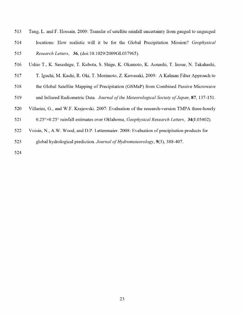
513 Tang, L. and F. Hossain. 2009: Transfer of satellite rainfall uncertainty from gauged to ungauged
514 locations: How realistic will it be for the Global Precipitation Mission'? Geophysical
515 Research Letters, 36, (do1:10.1029/2009GL037965).
516 Ushio T., K. Sasashige, T. Kubota, S. Shige, K. Okamoto, K. Aonashi, T. Inoue, N. Takahashi,
517 T. Iguchi, M. Kachi, R. Oki, T. Morimoto, Z. Kawasaki, 2009: A Kalman Filter Approach to
518 the Global Satellite Mapping of Precipitation (GSMaP) from Combined Passive Microwave
519 and Infrared Radiometric Data. Jornrnal of the Meteorological Society ofJapan, 87, 137-151.
520 Villarim, G., and W.F. Krajewski. 2007: Evaluation of the research-version TMPA three-hourly
521 0.25°X0.25° rainfall estimates over Oklahoma, Geophysical Research Letters, 34(L05402).
522 Voisin, N., A.W. Wood, and D.P. Lettenmaier. 2008: Evaluation of precipitation products for
523 global hydrological prediction. Journal of Hvdronieteorology, 9(3), 388-407.
524
23
525
LIST OF FIGURE CAPTIONS
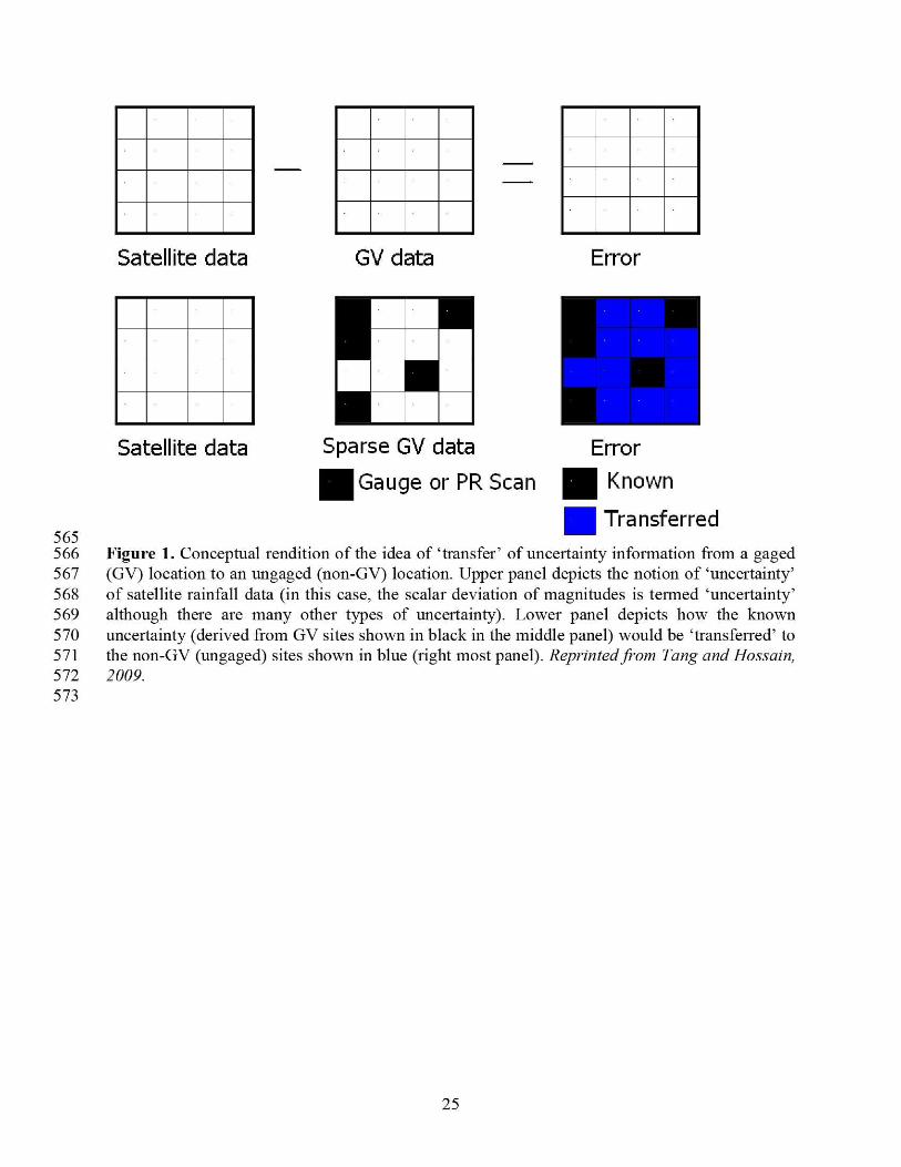
Figure 1. Conceptual rendition of the idea of `transfer' of uncertainty information from a gaged(GV) location to an ungaged (non-GV) location. Upper panel depicts the notion of `uncertainty'of satellite rainfall data (in this case, the scalar deviation of magnitudes is termed `uncertainty'although there are many other types of uncertainty). Lower panel depicts how the knownuncertainty (derived from GV sites shown in black in the middle panel) would be `transferred' tothe non-GV (ungaged) sites shown in blue (right most panel). Reprinted from Tang and Hossain,2009.
Figure 2. Correlation length of uncertainty metrics at climatologic timescales for 31341 RT(upper panel) and 31342RT (lower panel) shown as a function of season. Note the distance unit is0.25 degree grid boxes (-- 25 km). The vertical bars are shown in order from left to right as`Bias', `RMSE', `POD rain', `POD no-rain', `FAR'. (Taken from Tang and Hossain, 2009).
Figure 3. Left panels: probability of a 31342RT 0.25 0 grid box having a PMW scan from eitherTMI, SSMIs or AMSR for 3 hour (upper), 6 hour (middle), and 24 hour periods (bottom). Rightpanels: Same as left panels but only for TMI.
Figure 4a. Transfer of Bias of 31341RT from gauged to ungauged locations. Upper left-mostpanel shows the true field of uncertainty in bias based on 6 years of data. The lower left-mostpanel is the randomly selected 50% of the region for computation of the empirical variogram andcorrelation length. The lower middle panel shows the other 50% of the region that was assumedhave no GV. Lower right panel shows the estimation of the bias at the non-GV grid boxes usingordinary kriging.
Figure 4b. Histograms of kriging error and actual error for false alarm ratio (FAR) overungauged gridboxes. Here kriging error (shown in black) is defined as the difference betweentransferred (or kriged) FAR and the actual FAR derived from GV data. The actual GV-basedFAR is shown in pink.
Figure 4b. Histograms of kriging error and actual error for false alarm ratio (FAR) overungauged gridboxes. Here kriging error (shown in black) is defined as the difference betweentransferred (or kriged) FAR and the actual FAR derived from GV data. The actual GV-basedFAR is shown in pink.
Figure 5. Impact of GV coverage (or sparseness) on the effectiveness of uncertainty metrictransfer by ordinary kriging at climatologic scale (upper panel) and seasonal scale (lower panel)for the central US.. Computed with TMPA data collected for a 100 day period (May-August) in2007-2008.
24
Satellite data
GV data
Error
Satellite data Sparse GV data ErrorMGauge or PR Scan Known
565Transferred
566 Figure 1. Conceptual rendition of the idea of `transfer' of uncertainty information from a gaged567 (GV) location to an ungaged (non-GV) location. Upper panel depicts the notion of `uncertainty'568 of satellite rainfall data (in this case, the scalar deviation of magnitudes is termed `uncertainty'569 although there are many other types of uncertainty). Lower panel depicts how the known570 uncertainty (derived from GV sites shown in black in the middle panel) would be `transferred' to571 the non-GV (ungaged) sites shown in blue (right most panel). Reprinted fr •oni Tang and Hossain,572 2009.573
25
3841 R Analysis on Spatial Structure per Season(Correlation Length)
5
.4- -
Spring.14arch-Maytc3
Summer: June-August vc.0
September-November ro iv
Winter. December-February
0S! dng I Surrrmer Faii tl'vttE
T me period q Bi as 3.9 2.2 2 4 3.92002-2007 q R 5f 4 2.5 2, 7 2,9Units: q ?017 of rain 2.7 2. 5 2,3 2. 10 25 degree p pgD of no rain 3.4 2 9 3.5 3,3
q F!1R 2.7 1. 9 2.2 4. 4
3842RT Analysis on Spatial Structure per Season(Correlation Length)
3
2.5
Spring: PAarch-10ay 2c - -
Summer. June-August-01.5
Fall. September-November^ 1
Winter December-February oU^5
0 -
Spring Summer Fa!; vlQnter
Time period. q :a 1. 466 S--
2002-2007 .R..- 2.2666 0 ; 9' 0T---
Units: q ?OD cf : ein 2.268 616 T." degree q ?OD c z',, T. 766 21 464 516 1.53..
q . R =99 661 1 2.90,--
Figure 2. Correlation length of uncertainty metrics for 3B41RT (upper panel)and 3B42RT (lower panel) shown as a function of season. Note the distanceunit is 0.25 degree grid boxes (— 25 km). The vertical bars are shown in orderfrom left to right as `Bias', `RMSE', `POD rain', `POD no-rain', `FAR'.(Taken fi •onl Tang and Hossain, 2009).
574
575
576
577
578
26
PROBABILITY OF MICROWAVE SCAN FOR 3B42RT PROBABILITY OF TMI SCAN FOR 3B42RT(2007 3 HOUR WINDOW) N (3 HOUR WINDOW) N
of
^^ dJ "' ^ ^:
n>~ 4,
d` lo
Y
0 1.100 1210 B.d00 Miles dd70 eP]0 n01es
i..ame
0 01 02 03 04 Os 06 07 06 09 I
L.a.^d
0 0.1 02 0.3 OA 05 0.6 01 C 09 I
PROBABILITY OF A MICROWAVE SCAN FOR 3B42RT(2007 6 HOUR WINDOW) N
PROBABILITY OF TMI SCAN FOR 3B42RT(6 HOUR WINDOW) N
0 1.100 ea10 Bp]O Mees
"9and0 0.1 03 03 OR 05 0.6 07 0.8 09 1
1,100 1¢0 fi.d00 Mlles
1. a
0 0.1 0.2 03 Oa 0.5 06 0? OB 09 I
PROBABILITY OF A MICROWAVE SCAN FOR 3B42RT(2007 24 HOUR WINDOW) N
PROBABILITY OF TMI SCAN FOR 3B42RT(24 HOUR WINDOW) N
A A^"-
1,100 eYM 6.600 Mile,
L.a d0 0.1 0.1 03 0.4 05 0.8 OT 03 0.9 I
0 tIW e]00 B.tlO Mite
uo.ed0 0.1 02 03 0,4 0.8 06 0.7 08 09 I
Figure 3. Left panel: probability of a 3B42RT 0.25° grid box having a PMW scan from either TMI,SSMIs or AMSR for 3 hour (upper), 6 hour middle) and 24 hour periods (bottom). Right panel:Same as left panel but only for TMI. These probability maps were created using a 100 day period ofany PMW sensor from the 2007- 2008 period.
579
580
27
581
582
Original data
^L n
LML-
t
Iti
iPMi • ^. ' ^^ ^^
'WW rw. 95,W W.
3B41RT BIAS
Kriging result.5'N
15' N
16
SUI'W :JC'W 99'W 90'W
Units. mnVhr
M-005-0025_ -0024-0005_0005-002-0.02.003=0.03-004Ci 0.04 - 0.05M0.05-006-0.06-007-007-008_ 008-011
Known data Unknown data (original).S• N — _ .rN
r l
Lz
ON J6 Arm X
.^
1KW ]UO'W 9S'W 9p'w ,.q-W 1W W 95'w W"
Unknown data (kriging)
41 ir
9S "V.- Aq-r,
'n
.rF •r;
r ^i71 '^ ^.^ 1 7
9S•N ^ I1 6.. ^.y
L .Y
—^W. foo'w 9r.•. Ww
5 83584 Figure 4a. Transfer of Bias of 3B41RT from gauged to ungauged locations. Upper leftmost585
panel shows the true field of uncertainty on bias based on 6 years of data. The lower left most586
panel is the randomly selected 50% of the region for computation of the empirical variogram and587
correlation length. The lower middle panel shows the other 50% of the region that was assumed588
to be non-GV grid boxes. Lower right panel shows the estimation of the bias at the non-GV grid589
boxes using ordinary kriging.590
28
3 B42 RT- MEH st ogr am of Data and Kr i gi ng Errors
T —— FY obabi I i t y of Kr i gi ng ErrorsR nhahi I i t v of rlat a val ups
0 0.1 0.2 0.3 0.4 0.5 0.6 0.7 0.8 0.9 1 1.1 1.2
R VSE val ues or errors ( and hr)
6%
5%
4%
3%
2%
1%
0%
-0.4 -0.3 -0.2 -0.1
591592593594595596597598599600601602603604605606607608609610611612613614
Figure 4b. Histograms of kriging error and actual uncertainty for false alarm ratio (FAR) overungauged gridboxes. Here kriging error (shown in black) is defined as the difference betweentransferred (or kriged) FAR and the actual FAR derived from GV data. The actual GV-basedFAR is shown in pink.
29
Climatologic Scale (6 years)1
d ia_^ m 0.9
Y t BIAS'aca 0.8 RMSE
a POD0.7t
3^ U
0.62
U E0.5
10 20 30 40 50 60 70 80 90
% of region lacking GV data
Seasonal Scale (3 months)
1 - -
p UCD, a 0.9 = - _-
Y EC ^ _
3 a 0.8 -
NtBIASc -a 0.7 (RMSEO cR U POD
0.6o °i
EU
0.5
10 20 30 40 50 60 70 80 90
% of region lacking GV data
Figure 5. Impact of GV coverage (or sparseness) on the effectiveness of uncertaintymetric transfer by ordinary kriging at climatologic scale (upper panel) and seasonal scale(lover panel) for the central US.
615
616
617
30
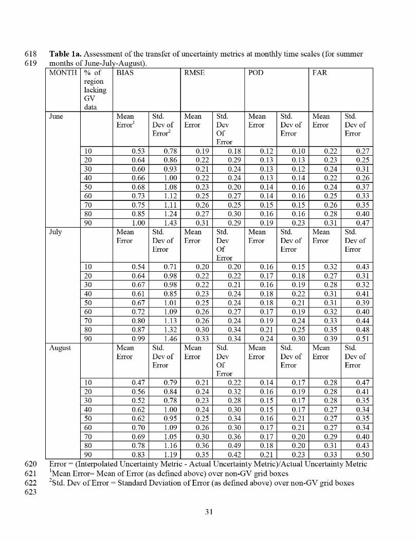
618 Table la. Assessment of the transfer of uncertainty metrics at monthly time scales (for summer619 months of June-July-August).
MONTH % ofregionlackingGVdata
BIAS RMSE POD FAR
June MeanError'
Std.Dev ofError2
MeanError
Std.DevOfError
MeanError
Std.Dev ofError
MeanError
Std.Dev ofError
10 0.53 0.78 0.19 0.18 0.12 0.10 0.22 0.2720 0.64 0.86 0.22 0.29 0.13 0.13 0.23 0.2530 0.60 0.93 0.21 0.24 0.13 0.12 0.24 0.3140 0.66 1.00 0.22 0.24 0.13 0.14 0.22 0.2650 0.68 1.08 0.23 0.20 0.14 0.16 0.24 0.3760 0.73 1.12 0.25 0.27 1 0.14 0.16 0.25 0.3370 0.75 1.11 0.26 0.25 0.15 0.15 0.26 0.3580 0.85 1.24 0.27 0.30 0.16 0.16 0.28 0.4090 1.00 1_43 0.31 0.29 0.19 0.23 0.31 0.47
July MeanError
Std.Dev ofError
MeanError
Std.DevOfError
MeanError
Std.Dev ofError
MeanError
Std.Dev ofError
10 0.54 0.71 0.20 0.20 0.16 0.15 0.32 0.4320 0.64 0.98 0.22 0.22 0.17 0.18 0.27 0.3130 0.67 0.98 0.22 0.21 0.16 0.19 0.28 0.3240 0.61 0.85 0.23 0.24 0.18 0.22 0.31 0.4150 0.67 1.01 0.25 0.24 0.18 0.21 0.31 0.3960 0.72 1.09 0.26 0.27 0.17 0.19 0.32 0.4070 0.80 1.13 0.26 0.24 0.19 0.24 0.33 0.4480 0.87 1_32 0.30 0.34 0.21 0.25 0.35 0.4890 0.99 1.46 0.33 0.34 0.24 0.30 0.39 0.51
August MeanError
Std.Dev ofError
MeanError
Std.DevOfError
MeanError
Std.Dev ofError
MeanError
Std.Dev ofError
10 0.47 0.79 0.21 0.22 0.14 0.17 0.28 0.4720 0.56 0.84 0.24 0.32 0.16 0.19 0.28 0.4130 0.52 0.78 0.23 0.28 0.15 0.17 0.28 0.3540 0.62 1.00 0.24 0.30 0.15 0.17 0.27 0.3450 0.62 0.95 0.25 0.34 0.16 0.21 0.27 0.3560 0.70 1.09 0.26 0.30 0.17 0.21 0.27 0.3470 0.69 1 1.05 1 0.30 1 0.36 1 0.17 1 0.20 0.29 0.4080 0.78 1.16 0.36 0.49 0.18 0.20 0.31 0.4390 0.83 1.19 0.35 0.42 0.21 0.23 0.33 0.50
620 Error = (Interpolated Uncertainty Metric - Actual Uncertainty Metric)/Actual Uncertainty Metric621 1 Mean Error= Mean of Error (as defined above) over non-GV grid boxes622 ZStd. Dev of Error = Standard Deviation of Error (as defined above) over non-GV grid boxes623
31
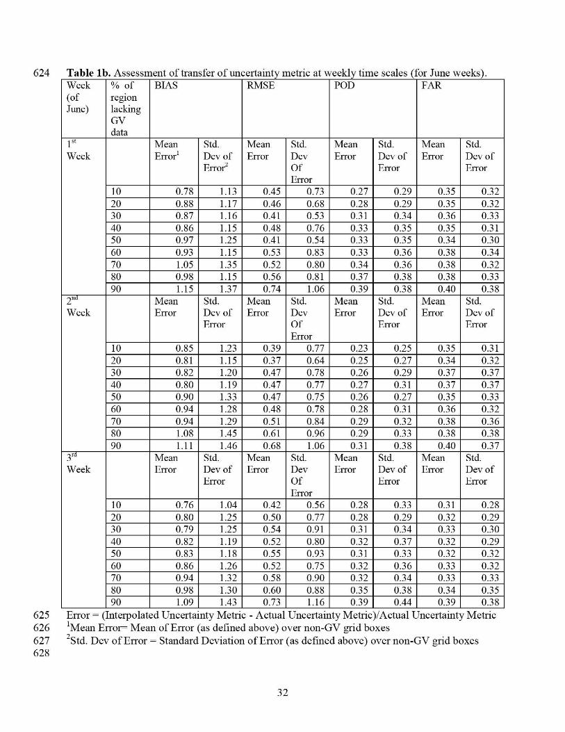
624 Table lb. Assessment of transfer of uncertainty metric at weeklv time scales (for June weeks).Week(ofJune)
% ofregionlackingGVdata
BIAS RMSE POD FAR
lst
WeekMeanError'
Std.Dev ofError
MeanError
Std.DevOfError
MeanError
Std.Dev ofError
MeanError
Std.Dev ofError
10 0.78 1.11) 0.45 0.73 0.27 0.29 0.35 0.32
20 0.88 1.17 0.46 0.68 0.28 0.29 0.35 0.3230 0.87 1.16 0.41 0.53 0.31 0.34 0.36 0.33
40 0.86 1.15 0.48 0.76 0.33 0.35 0.35 0.3150 0.97 125 0.41 0.54 0.33 0.35 0.34 0.30
60 093 1.15 0.53 1 0.83 0.33 0.36 0.38 0.34
70 1.05 135 0.52 0.80 034 0.36 0.38 0.3280 0.98 1.15 0.56 0.81 0.37 0.38 0.38 0.33
90 1.15 1.37 0.74 1.06 0.39 0.38 0.40 0.382 nd
WeekMeanError
Std.Dev ofError
MeanError
Std.DevOfError
MeanError
Std.Dev ofError
MeanError
Std.Dev ofError
10 0.85 1.23 0.39 0.77 0.23 0.25 0.35 0.31
20 0.81 1.15 037 0.64 0.25 0.27 0.34 0.3230 0.82 120 0.47 0.78 0.26 0.29 0.37 0.37
40 0.80 1.19 0.47 0.77 0.27 0.31 0.37 0.3750 090 1.33 0.47 0.75 0.26 0.27 0.35 0.33
60 0.94 128 0.48 0.78 0.28 0.31 0.36 0.32
70 094 1.29 0.51 0.84 1 0.29 0.32 0.38 0.3680 1.08 1.45 0.61 0.96 0.29 0.33 0.38 0.38
90 1.11 1.46 0.68 1.06 0.31 0.38 0.40 0.373 rd
WeekMeanError
Std.Dev ofError
MeanError
Std.DevOfError
MeanError
Std.Dev ofError
MeanError
Std.Dev ofError
10 0.76 1.04 0.42 0.56 0.28 0.33 0.31 0.28
20 0.80 1.25 0.50 0.77 0.28 0.29 0.32 0.2930 0.79 1.25 0.54 0.91 0.31 0.34 0.33 0.30
40 0.82 1.19 0.52 0.80 0.32 0.37 0.32 0.2950 0.83 1.18 0.55 0.93 0.31 0.33 0.32 0.32
60 0.86 1.26 0.52 0.75 0.32 0.36 0.33 0.3270 0.94 1.32 0.58 0.90 0.32 0.34 0.33 0.33
80 0.98 1.30 0.60 0.88 0.35 0.18 0.14 0.3590 1.09 1.43 0.73 1.16 0.39 0.44 0.39 0.38
625 Error = (Interpolated Uncertainty Metric - Actual Uncertainty Metric)/Actual Uncertainty Metric626 'Mean Error= Mean of Error (as defined above) over non-GV grid boxes627 2 Std. Dev of Error = Standard Deviation of Error (as defined above) over non-GV grid boxes628
32
NA (HIT) NB (MISS)
NC (MISS) ND (HIT)
x
w
N
635
636
637
638
639
640
641
M u
^ xi OG '^
Z U
629 Table A.1. Contingency Table (a HIT is defined when both satellite and GV agree on the type of630 event detected; a MISS is when there is disagreement between satellite and GV detected events).631
632
633 Truth/Reference
634 Rainy Gridboxes Non-rainy Gridboxes
33