Transfer Learning in Computer Vision Tasks:

Remember Where You Come From

Xuhong Lia, Yves Grandvaleta, Franck Davoinea, Jingchun Chengb, YinCuic, Hang Zhangd, Serge Belongiec, Yi-Hsuan Tsaie, Ming-Hsuan Yangf

aAlliance Sorbonne Universite, Universite de technologie de Compiegne, CNRS,Heudiasyc, UMR 7253, Compiegne, France.

bTsinghua UniversitycCornell University

dAmazon InceNEC Labs America

fUniversity of California at Merced

Abstract

Fine-tuning pre-trained deep networks is a practical way of benefiting fromthe representation learned on a large database while having relatively fewexamples to train a model. This adjustment is nowadays routinely per-formed so as to benefit of the latest improvements of convolutional neuralnetworks trained on large databases. Fine-tuning requires some form of reg-ularization, which is typically implemented by weight decay that drives thenetwork parameters towards zero. This choice conflicts with the motivationfor fine-tuning, as starting from a pre-trained solution aims at taking advan-tage of the previously acquired knowledge. Hence, regularizers promotingan explicit inductive bias towards the pre-trained model have been recentlyproposed. This paper demonstrates the versatility of this type of regular-izer across transfer learning scenarios. We replicated experiments on threestate-of-the-art approaches in image classification, image segmentation, andvideo analysis to compare the relative merits of regularizers. These testsshow systematic improvements compared to weight decay. Our experimentalprotocol put forward the versatility of a regularizer that is easy to implementand to operate that we eventually recommend as the new baseline for futureapproaches to transfer learning relying on fine-tuning.

Keywords: Transfer learning, parameter regularization, computer vision

Preprint submitted to Image and Vision Computing October 24, 2019

1. Introduction

The L2 parameter regularization, also known as weight decay, is com-monly used in machine learning and especially when training deep neuralnetworks. This simple regularization scheme restricts the capacity of thetrained model by restraining the e↵ective size of the search space duringoptimization, implicitly driving the parameters towards the origin. Whenhaving no a priori knowledge about the “true solution”, the origin is an arbi-trary yet reasonable choice. However, the parameters can be driven towardsany value of the parameter space, and better results should be obtained fora value closer to the true one [12, Section 7.1.1].

Li et al. [21] recently proposed to use the pre-trained model as an a prioriknowledge about the “true solution” in transfer learning: the starting point(-SP) should be used in place of the origin as the reference for parameter reg-ularization. Figure 1 illustrates this scheme in a simple case that correspondsto linear regression. The left-hand side plot (a) represents the weight decayregularizer when starting from the origin (no fine-tuning): the optimizer goestowards the solution of the unregularized risk and stops when reaching theboundary of the admissible set. The center plot (b) represents the weight-decay regularizer when starting from the pre-trained solution, assumed to bein the vicinity of the solution to the unregularized risk: the optimizer reachesthe previous solution; all the benefit of the pre-trained solution is lost. Theright-hand side plot (c) represents the L2

-SP regularizer: the optimizer con-verges towards a solution between the pre-trained solution and the solutionof the unregularized risk; the memory of the pre-trained solution is preserved.Note that the very same scenario is unlikely with non-convex deep models,but it seems dangerous to rely on non-convexity to prevent forgetting.

Li et al. [21] showed that the -SP regularizers improve transfer learning inimage classification. However, weight decay still remains predominantly usedin computer vision for fine-tuning, maybe due to the limited experimentalevidence of the benefit of -SP regularizers. In this paper, we aim at demon-strating the general usefulness of L2

-SP for transfer learning, by providingnovel evidences showing that the simple L2

-SP regularizer is applicable in avery wide scope.

The following sections provide the necessary background material regard-ing transfer learning (Section 2), regularizers (Section 3) and the tested ap-proaches (Section 4). We then report in Section 5 a wide variety of ex-periments, dealing with state-of-the-art transfer learning schemes for image

2

(a) (b) (c)

Figure 1: Inadequacy of the standard L2 regularization for transfer learning. Each plotshows the same 2D parameter space in a simple transfer learning situation. The red starrepresents the minimum of the unregularized risk for the target problem; the black crossis the starting point of the optimization process, and the black point represents the resultof a gradient-like optimizer, with intermediate solutions represented by the black segment.The ellipses represent the contour levels of the target problem, and the large blue circlerepresents the e↵ective search domain defined by the regularizer (admissible set). Thesub-figures correspond to: (a) the standard learning process with L2 regularization (nofine-tuning), (b) the fine-tuning process with L2 regularization, (c) the fine-tuning processwith L2-SP regularization.

classification (DSTL [7], short for domain similarity for transfer learning),image segmentation (EncNet [45]) and video analysis (SegFlow [5]). In orderto avoid any form of experimental bias, all the experiments reported in thispaper were carried out under the exact conditions of the original transferlearning schemes, by the main authors of the original approaches, who in-troduced a single modification in the fine-tuning protocol, by replacing L2

by L2-SP regularization. These experimental results show consistent im-

provement for L2-SP regularization, demonstrating the versatility of the -SP

regularizers for fine-tuning across network structures, datasets, and visionproblems. These improvements are marginal to moderate, but should not beneglected since they come with minimal computing overhead. We thus claimthat L2

-SP regularization should be adopted as a baseline, or in combinationwith other schemes in all vision applications relying on transfer learning.

2. Related Work

2.1. Inductive Transfer Learning

Regarding transfer learning, we follow the nomenclature of Pan and Yang[32]. A domain corresponds to the feature space and its distribution, whereas

3

a task corresponds to the label space and its conditional distribution withrespect to features. The initial learning problem is defined on the sourcedomain and the source task, whereas the new learning problem is defined onthe target domain and the target task. According to domain and task set-tings during the transfer, Pan and Yang categorized several types of transferlearning problems. Inductive transfer learning is the situation where the tar-get domain is identical to the source domain and the target task is di↵erentfrom the source task. Many recent applications of convolutional networks,like image classification [11, 7], object detection [35, 46, 24], object instancesegmentation [14, 15, 25], image segmentation [5, 45, 4], depth estimation[26, 6], optical flow [16, 5, 20], human action recognition [47, 3], and personre-identification [34, 17], rely on transfer learning in the inductive transferlearning setting. All these approaches start with some model pre-trained ona source domain for image classification and fine-tune them on the targetdomain for a di↵erent task. They show state-of-the-art results in a challeng-ing transfer learning setup, as going from classification to object detectionor image segmentation requires notable modifications in the architecture ofthe network.

The success of these approaches relies on the generality of the repre-sentations that have been learned from a large database like ImageNet [8].Yosinski et al. [44] quantify the transferability of these pieces of informationin di↵erent layers, i.e. the first layers learn general features, the middle layerslearn high-level semantic features and the last layers learn the features thatare very specific to a particular task. Overall, the learned representations canbe conveyed to related but di↵erent domains and the network parameters arereusable for di↵erent tasks.

2.2. Parameter Regularizers for Transfer Learning

Parameter regularization is widespread in deep learning. L2 regulariza-tion has been used for a long time as a simple method for preventing overfit-ting by limiting the norm of the parameter vector. Besides L2, other penaltieshave been proposed, such as max-norm regularization [38], which is foundespecially helpful when using dropout, or the orthonormal regularizer [43],which forces each kernel in one convolution layer to have minimum correlationwith others.

The L2-SP regularization we consider in this paper has been used in

lifelong learning [22, 18] to cope with the catastrophic forgetting problem. Asimilar regularizer has also been used in domain adaptation for vision [36],

4

speaker adaptation [23, 31], and neural machine translation [1]. In brief,L2

-SP is an explicit inductive bias towards the initial parameters that hasbeen proved to be useful in di↵erent transfer learning scenarios. However,weight decay remains predominantly used in the computer vision communityfor fine-tuning.

3. A Reminder on -SP regularizers

The regularizers that were recently proposed in [21] apply to the vectorw 2 Rn containing all the network parameters that are to be adapted tothe target task. The regularized objective function J that is to be opti-mized is the sum of the standard objective function J and the regularizer⌦(w). In practice, J is usually the negative log-likelihood, so that the cri-terion J could be interpreted in terms of maximum a posteriori estimation,where the regularizer ⌦(w) would act as the log prior of w. More generally,the minimization of J is a trade-o↵ between the data-fitting term and theregularization term.

L2penalty. The current baseline penalty for transfer learning is the L2

penalty, also known as weight decay:

⌦(w) =↵

2kwk22 , (1)

where ↵ is the regularization parameter setting the strength of the penaltyand k·kp is the p-norm of a vector.

L2-SP. Let w0 be the parameter vector of the model pre-trained on the

source problem, acting as the starting point (-SP) in fine-tuning. Using thisinitial vector as the reference in the L2 penalty, we get:

⌦(w) =↵

2

��w �w0��2

2. (2)

Typically, the transfer to a target task requires some modifications of thenetwork architecture used for the source task, such as on the last layer usedfor predicting the outputs. Then, there is no one-to-one mapping betweenw and w0, and we use two penalties: one for the part of the target networkthat shares the architecture of the source network, denoted wS , the otherone for the novel part, denoted wS . The compound penalty then becomes:

⌦(w) =↵

2

��wS �w0S��2

2+

�

2kwSk

22 . (3)

5

Several other -SP regularizers exist, like L2-SP-Fisher or Group-Lasso-

SP [21], but we focus here on comparing L2 with L2-SP, because of the

simplicity and e�ciency of L2-SP compared to the other -SP regularizers.

4. Transfer Learning Approaches

In this section, we present the three recent representative approaches oftransfer learning with convolutional networks that will be used to comparethe L2 and L2

-SP regularizers. They cover a variety of setups, and theirprotocols rely at least partly on fine-tuning, originally implemented withweight decay.

4.1. EncNet

Zhang et al. [45] designed a context-encoding module to extract the re-lation between the object categories and their global semantic context inthe image, so as to emphasize the frequent objects in one context and de-emphasize the rare ones. The proposed module explicitly captures contextualinformation of the scene using sparse encoding and learns a set of scaling fac-tors, by which the feature maps are then rescaled for selectively highlightingthe class-dependent feature channels. For an image segmentation problem,the features highlighted by the semantic context facilitate the pixel-wise pre-diction and improve the recognition of small objects. Meanwhile, an auxiliaryloss is computed from the encoded features to better extract the contextualinformation.

We refer to this approach as EncNet, following [45]. It relies on a pre-trained ResNet [13] that is then evaluated on the PASCAL-Context dataset[10] for image segmentation.

4.2. SegFlow

Cheng et al. [5] constructed a network architecture, named SegFlow, withtwo branches for simultaneously (i) segmenting video frames pixel-wisely and(ii) computing the optical flow in videos. The segmentation branch is basedon ResNet [13] transformed into a fully-convolutional structure, while theoptical flow branch is an encoder-decoder network [9]. Both segmentationand optical flow branches have feature maps at multiple scales, enablingconnections between the two tasks. Gradients from both tasks can passthrough the two branches, and the last representations in feature space areshared.

6

SegFlow is initialized with two pre-trained networks: ResNet [13] for theencoding of the segmentation branch and FlowNetS [9] for the optical flowbranch. It is then fine-tuned on the DAVIS 2016 dataset [33] for video objectsegmentation and the Scene Flow datasets [28] for optical flow.

4.3. Domain Similarity for Transfer Learning

Cui et al. [7] measure the similarity between the source domain, supposedto cover a broad range of objects, and the target domain, supposed to be morespecific. They use the Earth Mover’s Distance to compute the similaritybetween the source categories and the target domains. They then choose thetop k categories of the source domain that best cover the target domains topre-train the network from scratch.

The networks are pre-trained on subsets of ImageNet [8] and iNatural-ist [41]. Here, we use their Subset B. This pre-trained network is then fine-tuned on di↵erent target databases (see Table 2). We refer to this approachas DSTL, the abbreviation of domain similarity for transfer learning.

5. Experiments

In this section, we experiment the three approaches, i.e. EncNet [45],SegFlow [5], and DSTL [7], with their original L2 penalty implementation,and compare their performances with the L2

-SP penalty, in the very sameexperimental conditions. To ensure perfect replication of the original proto-col, these experiments were carried out by the main authors of the originalpapers to avoid any kind of “competence bias”.

When these experiments are carried out using the L2 penalty, the fluctua-tions from the original results are only due to the inherent randomness of thestochastic learning process. When using the L2

-SP penalty, this is the onlypiece of code that was changed, and the very same conditions are observedotherwise, so as to ensure that di↵erences in performances are only due tothe di↵erences between the two regularization approaches during fine-tuning.

5.1. Experimental Setup

Datasets. The characteristics of the source and target datasets are summa-rized in Table 1 and Table 2 respectively, including the size of each dataset,the task related and the approach that uses this dataset. Note that DSTL in-cludes a scheme for building a source domain by selecting a subset of classesthat are the most relevant to the target task, but it follows a fine-tuningtransfer learning protocol nevertheless.

7

dataset

#im

ages/scen

es#classes

task

addressed

note

appro

ach

ImageN

et[8]

⇠1.2M

1000

imageclassification

object-centered

all

iNaturalist

[41]

⇠675K

5,089

imageclassification

naturalcategories

DSTL

FlyingChairs

[9]

⇠2K

scenes

-op

ticalflow

synthetic

SegFlow

Tab

le1:

Sou

rcedatasets:

number

ofexam

ples,nu

mber

ofclasses,typeof

task

addressed,an

dtheap

proach(es)

relyingon

this

dataset

asasourcetask.

dataset

#im

ages/seq.

#classes

task

addressed

appro

ach

PASCAL-C

ontext

[29]

⇠10K

59im

agesegm

entation

EncN

etSceneFlow

[28]

32sequ

ences

-op

ticalflow

SegFlow

DAVIS

2016

[33]

50sequ

ences

-video

segm

entation

SegFlow

CUB200[42]

⇠11K

200

imageclassification

DSTL

Flowers102

[30]

⇠10K

102

imageclassification

DSTL

Stanford

Cars[19]

⇠16K

196

imageclassification

DSTL

Aircraft[27]

⇠10K

100

imageclassification

DSTL

Foo

d101[2]

⇠100K

101

imageclassification

DSTL

NABirds[40]

⇠50K

555

imageclassification

DSTL

Tab

le2:

Targetdatasets:

number

ofexam

ples,nu

mber

ofclasses,typeof

task

addressed,an

dap

proachthat

usesthisdataset

asatarget

task.

8

Network Structures. The source task is usually a classification task, whichalleviates the labeling burden. Conventionally, if the target task is also clas-sification, like DSTL, the fine-tuning process starts by replacing the last layerwith a new one, randomly generated, with a size defined by the number ofclasses in the target task. The modification of the network structure in quitelight in this situation.

In contrast, for image segmentation and optical flow estimation, wherethe objectives di↵er radically from image classification, the source networkneeds to be modified, typically by adding a decoder part, which is muchmore involved than a single fully connected layer. Here, we follow exactlythe original papers regarding the modifications of the network architectures.

Training Details. For training details, we refer the reader to the originalpapers [5, 45, 7], since again, nothing was changed on this matter. Notethat L2 and L2

-SP are only applied to weights in convolutional and fullyconnected layers: the normalization layers or the biases are not penalized tofollow the usual fine-tuning protocol.

Evaluation Metrics. We briefly recall the evaluation metrics used for measur-ing the performance on these tasks. In image classification and segmentation,accuracy or pixel accuracy is defined as the ratio of correctly predicted ex-amples or pixels to the total.

In segmentation, performance is evaluated by the mean intersection over

union (mean IoU or mIoU). The intersection over union (IoU) compares twosets: the set of pixels that are predicted to be of a given category and theset of pixels that truly belong to this category. It measures the discrepancybetween the two sets as the ratio of their intersection to their union. ThemIoU is the mean of IoUs over all categories.

In optical flow, performance is evaluated by the average endpoint error

(EPE) is defined as the average L2 distance between the estimated opticalflow and the ground truth at each pixel.

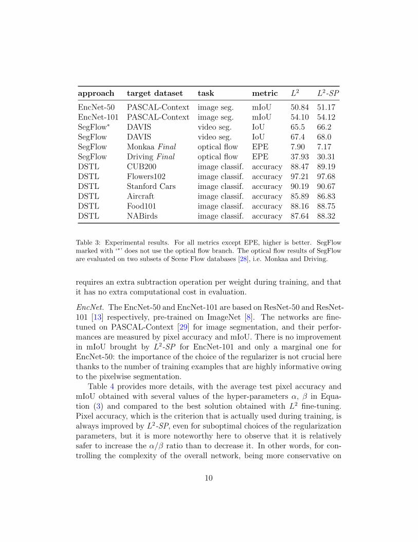
5.2. Experimental Results

Table 3 compares the results of fine-tuning with L2 and L2-SP of all

approaches on their specific target tasks. We readily observe that fine-tuningwith L2

-SP in place of L2 consistently improves the performance, whateverthe task, whatever the approach. Some of these improvements are marginal,but we recall that, compared to the L2 fine-tuning baseline, L2

-SP only

9

approach target dataset task metric L2 L2-SP

EncNet-50 PASCAL-Context image seg. mIoU 50.84 51.17EncNet-101 PASCAL-Context image seg. mIoU 54.10 54.12SegFlow⇤ DAVIS video seg. IoU 65.5 66.2SegFlow DAVIS video seg. IoU 67.4 68.0SegFlow Monkaa Final optical flow EPE 7.90 7.17SegFlow Driving Final optical flow EPE 37.93 30.31DSTL CUB200 image classif. accuracy 88.47 89.19DSTL Flowers102 image classif. accuracy 97.21 97.68DSTL Stanford Cars image classif. accuracy 90.19 90.67DSTL Aircraft image classif. accuracy 85.89 86.83DSTL Food101 image classif. accuracy 88.16 88.75DSTL NABirds image classif. accuracy 87.64 88.32

Table 3: Experimental results. For all metrics except EPE, higher is better. SegFlowmarked with ‘⇤’ does not use the optical flow branch. The optical flow results of SegFloware evaluated on two subsets of Scene Flow databases [28], i.e. Monkaa and Driving.

requires an extra subtraction operation per weight during training, and thatit has no extra computational cost in evaluation.

EncNet. The EncNet-50 and EncNet-101 are based on ResNet-50 and ResNet-101 [13] respectively, pre-trained on ImageNet [8]. The networks are fine-tuned on PASCAL-Context [29] for image segmentation, and their perfor-mances are measured by pixel accuracy and mIoU. There is no improvementin mIoU brought by L2

-SP for EncNet-101 and only a marginal one forEncNet-50: the importance of the choice of the regularizer is not crucial herethanks to the number of training examples that are highly informative owingto the pixelwise segmentation.

Table 4 provides more details, with the average test pixel accuracy andmIoU obtained with several values of the hyper-parameters ↵, � in Equa-tion (3) and compared to the best solution obtained with L2 fine-tuning.Pixel accuracy, which is the criterion that is actually used during training, isalways improved by L2

-SP, even for suboptimal choices of the regularizationparameters, but it is more noteworthy here to observe that it is relativelysafer to increase the ↵/� ratio than to decrease it. In other words, for con-trolling the complexity of the overall network, being more conservative on

10

approach ↵ � accuracy mIoU

EncNet-50 - L2 1e-4 1e-4 79.09 50.84EncNet-50 - L2

-SP 1e-4 1e-3 79.10 50.31EncNet-50 - L2

-SP 1e-3 1e-4 79.18 51.12EncNet-50 - L2

-SP 1e-4 1e-4 79.20 51.17

EncNet-101 - L2 1e-4 1e-4 80.70 54.10EncNet-101 - L2

-SP 1e-4 1e-4 80.81 54.12

Table 4: EncNet pixel accuracy and mIoU on the PASCAL-Context validation set accord-ing to regularization hyper-parameters.

the pre-trained part of the network is a better option than being more con-strained on its novel part.

SegFlow. As for the segmentation performance of SegFlow, we have con-ducted two experiments: fine-tuning without the optical flow branch (de-noted SegFlow⇤ in Table 3) and fine-tuning the entire model. Both optionsare evaluated on the DAVIS target task [33]. The segmentation branch andthe optical flow branch of SegFlow are pre-trained on ImageNet [8] and Fly-ingChairs [9] respectively. When applicable, both branches are regularizedby L2 fine-tuning or towards the pre-trained values by L2

-SP fine-tuning.The benefits of L2

-SP are again systematic and higher for SegFlow⇤, whereless data is fed to the network during fine-tuning.

For the optical flow estimation, we also observe systematic benefits ofL2

-SP (recall that, for the EPE measure, the lower, the better), with againhigher impact for the smaller target training set Driving, that only comprises8 scenes. Table 5 reports additional results on two subsets of the Scene FlowDataset [28]: Monkaa, based on an animated short film, with 24 scenes, andDriving, containing 8 realistic driving street scenes. There are two versionsfor both datasets: a Clean version, which has no motion blur and atmospherice↵ects and a Final version, with blurring and e↵ects. Table 5 displays resultsfor di↵erent choices of � when using L2

-SP during fine-tuning. Comparedto L2, L2

-SP performs better on a wide range of � values, covering severalorders of magnitude, showing that suboptimal choices of (↵, �) still allowfor substantial reductions in errors. Hence, fine-tuning SegFlow with L2

-SP

does not require an intensive search of hyper-parameters.

11

�Monkaa Driving

Clean Final Clean Final

SegFlow-L2 7.94 7.90 37.91 37.93SegFlow-L2

-SP 1e0 7.55 7.60 34.20 35.17SegFlow-L2

-SP 1e-1 7.10 7.17 31.11 30.31SegFlow-L2

-SP 1e-2 7.41 7.52 30.57 30.14

Table 5: Average endpoint errors (EPEs) on the two subsets of the Scene Flow datasetaccording to the regularization hyper-parameter � (for ↵ = 0.1). The evaluations areperformed on the validation set of the Monkaa and Driving datasets and use both forwardand backward samples.

DSTL. The source datasets used here for DSTL are subsets of ImageNet [8]and iNaturalist [41], containing 585 categories slightly biased towards birdand dog breeds, i.e. Subset B in [7]. Inception-V3 [39] is pre-trained on thissubset and then fine-tuned on six target datasets. See Table 2 for the detailsof datasets.

Table 3 displays that fine-tuning with L2-SP improves systematically

upon the L2 baseline. We again investigate the sensitivity to hyper-parametersin Table 6 on the validation set of CUB200 [42], which is a dataset of 200bird species. As previously, the improved performance of the L2

-SP penaltyspans a wide area of values, and large ↵/� ratios are preferable to small ones.

approach ↵ � accuracy

DSTL - L2 4e-5 4e-5 88.47DSTL - L2

-SP 1e-4 1e-4 89.07DSTL - L2

-SP 1e-3 1e-3 89.19DSTL - L2

-SP 1e-3 1e-2 88.53DSTL - L2

-SP 1e-2 1e-3 89.12DSTL - L2

-SP 1e-1 1e-3 89.00

Table 6: DSTL classification accuracy using the Inception-V3 network on the CUB200validation set according to regularization hyper-parameters.

12

5.3. Analysis and Discussion

Behavior across Network Structures. L2-SP behaves very well across all tested

network structures. EncNet is based on ResNet [13] and modified by addinga context encoding module. The segmentation branch of SegFlow is basedon ResNet transformed to fully convolutional; the flow branch is FlowNetS[9], which is a variant of VGG [37]. For DSTL, Inception-V3 [39] is used.Throughout the various network structures and the diversity of problem ad-dressed, we consistently observe better performances with fine-tuning usingL2

-SP.

Choosing ↵ and �. The selection of the regularization parameters ↵ and �of Equation (3) does not require a precise search; a rule of thumb is to favorlarge ↵/� ratio rather than small ones: when transfer helps, the pre-trainedweights are relevant, and ↵ can be set to a large value without imposingdetrimental constraints. As for �, which applies to the randomly initializedweights in the new layers, a large � impedes the necessary adaptation.

Bias-Variance Analysis. We propose here a simple bias-variance analysis forthe tractable case of linear regression. Consider the squared loss functionJ(w) = 1

2kXw � yk2, where y 2 Rn is a vector of continuous responses,and X 2 Rn⇥p is the matrix of predictor variables. We use the standardassumptions of the fixed design case, that is: (i) y is the realization of arandom variable Y such that E[Y] = Xw⇤, V[Y] = �2In, and w⇤ is thevector of true parameters; (ii) the design is fixed and orthonormal, that is,XTX = Ip. We also assume that the reference we use for L2

-SP, i.e. w0, isnot far away from w⇤ (since it is the minimizer of the unregularized objectivefunction on a large data set): w0 = w⇤ + ", where ", the di↵erence betweenthe two parameters, is supposed to be relatively small, i.e. k"k ⌧ kw⇤k.

We consider the three estimates bw = argminwJ (w), bwL2

= argminwJ (w)+↵2 kwk22 and bwSP = argminwJ (w) + ↵

2 kw �w0k22. Their closed-form formu-lations, expectations and variances are given in Table 7. Without any regu-larization, the least squares estimate bw is unbiased, but with the largest vari-ance. With the L2 regularizer, variance is decreased by a factor of 1/(1 + ↵)2

but the squared bias is kw⇤k2↵2/(1 + ↵)2. The L2-SP regularizer benefits

from the same decrease of variance and su↵ers from the smaller squared biask"k2↵2/(1 + ↵)2. It is thus a better option than L2 (provided the assumptionk"k ⌧ kw⇤k holds), it is also always better than the least squares estimateprovided k"k < p�2 and otherwise better than this estimate for su�cientlysmall ↵, that is for ↵ < 2p�2/(k"k2 � p�2).

13

bw bwL2

bwSP

closed-form XTy 11+↵X

Ty 11+↵X

Ty + ↵1+↵w

0

E w⇤ 11+↵w

⇤ w⇤ + ↵1+↵"

V �2Ip�

�1+↵

�2Ip

��

1+↵

�2Ip

Table 7: Three estimates of the solution of a simple linear regression problem using dif-ferent regularizers, and their expectations E and variances V.

6. Conclusion

This paper provides new evidences on the relevance of the L2-SP regular-

ization in transfer learning. We report experiments with three representativestate-of-the-art transfer learning approaches of computer vision: EncNet [45],SegFlow [5], and DSTL [7]. Our protocol avoids any distortion or bias byhanding over the experiments to the original authors of these approaches.This protocol was made possible thanks to the ease of implementation of theL2

-SP regularization, whose adjustment is facilitated by the relative robust-ness with regard to the tuning of the regularization parameter. A generalsafe rule is to favor values of ↵ that are larger than �.

Our experiments demonstrate that fine-tuning with L2-SP regularization,

used in place of the standard weight decay, is e↵ective and versatile: not asingle comparison is in favor of fine-tuning with L2 regularization. Theseconclusions are not surprising, considering that fine-tuning is motivated byassuming the proximity of the solutions to the source and target problems.Our analysis in a simplified linear setting confirms that, when this assumptionis true, that is, when fine-tuning is expected to perform better than learningfrom scratch, L2

-SP is always better than L2. We thus conclude that L2-SP

regularization should be the baseline when fine-tuning for transfer learningin computer vision applications.

Acknowledgments

This work was carried out with the supports of the China ScholarshipCouncil and of a PEPS grant through the DESSTOPT project jointly man-aged by the National Institute of Mathematical Sciences and their Interac-

14

tions (INSMI) and the Institute of Information Science and their Interactions(INS2I) of the CNRS, France.

References

[1] Antonio Valerio Miceli Barone, Barry Haddow, Ulrich Germann, andRico Sennrich. Regularization techniques for fine-tuning in neural ma-chine translation. In Proceedings of the Conference on Empirical Meth-

ods in Natural Language Processing, pages 1489–1494, 2017.

[2] Lukas Bossard, Matthieu Guillaumin, and Luc Van Gool. Food-101–mining discriminative components with random forests. In European

Conference on Computer Vision (ECCV), pages 446–461, 2014.

[3] Joao Carreira and Andrew Zisserman. Quo vadis, action recognition? anew model and the kinetics dataset. In IEEE Conference on Computer

Vision and Pattern Recognition (CVPR), pages 4724–4733, 2017.

[4] Liang-Chieh Chen, Yukun Zhu, George Papandreou, Florian Schro↵,and Hartwig Adam. Encoder-decoder with atrous separable convolu-tion for semantic image segmentation. In Proceedings of the European

Conference on Computer Vision (ECCV), pages 801–818, 2018.

[5] Jingchun Cheng, Yi-Hsuan Tsai, Shengjin Wang, and Ming-Hsuan Yang.SegFlow: Joint learning for video object segmentation and optical flow.In IEEE International Conference on Computer Vision (ICCV), pages686–695, 2017.

[6] Xinjing Cheng, Peng Wang, and Ruigang Yang. Depth estimationvia a�nity learned with convolutional spatial propagation network. InProceedings of the European Conference on Computer Vision (ECCV),September 2018.

[7] Yin Cui, Yang Song, Chen Sun, Andrew Howard, and Serge Belongie.Large scale fine-grained categorization and domain-specific transferlearning. In IEEE Conference on Computer Vision and Pattern Recog-

nition (CVPR), pages 4109–4118, 2018.

15

[8] Jia Deng, Wei Dong, Richard Socher, Li-Jia Li, Kai Li, and Li Fei-Fei.Imagenet: A large-scale hierarchical image database. In IEEE Con-

ference on Computer Vision and Pattern Recognition (CVPR), pages248–255, 2009.

[9] Alexey Dosovitskiy, Philipp Fischer, Eddy Ilg, Philip Hausser, CanerHazirbas, Vladimir Golkov, Patrick Van Der Smagt, Daniel Cremers,and Thomas Brox. FlowNet: Learning optical flow with convolutionalnetworks. In IEEE Conference on Computer Vision and Pattern Recog-

nition (CVPR), pages 2758–2766, 2015.

[10] Mark Everingham, Luc Van Gool, Christopher KI Williams, John Winn,and Andrew Zisserman. The PASCAL visual object classes (VOC) chal-lenge. International Journal of Computer Vision, 88(2):303–338, 2010.

[11] Weifeng Ge and Yizhou Yu. Borrowing treasures from the wealthy: Deeptransfer learning through selective joint fine-tuning. In IEEE Conference

on Computer Vision and Pattern Recognition (CVPR), pages 10–19,2017.

[12] Ian Goodfellow, Yoshua Bengio, and Aaron Courville. Deep Learning.Adaptive Computation and Machine Learning. MIT Press, 2017.

[13] Kaiming He, Xiangyu Zhang, Shaoqing Ren, and Jian Sun. Deep resid-ual learning for image recognition. In IEEE Conference on Computer

Vision and Pattern Recognition (CVPR), pages 770–778, 2016.

[14] Kaiming He, Georgia Gkioxari, Piotr Dollar, and Ross Girshick. Mask R-CNN. In IEEE International Conference on Computer Vision (ICCV),pages 2980–2988, 2017.

[15] Hexiang Hu, Shiyi Lan, Yuning Jiang, Zhimin Cao, and Fei Sha. Fast-Mask: Segment multi-scale object candidates in one shot. In IEEE Con-

ference on Computer Vision and Pattern Recognition (CVPR), pages991–999, 2017.

[16] Eddy Ilg, Nikolaus Mayer, Tonmoy Saikia, Margret Keuper, AlexeyDosovitskiy, and Thomas Brox. Flownet 2.0: Evolution of optical flowestimation with deep networks. In IEEE Conference on Computer Vi-

sion and Pattern Recognition (CVPR), pages 2462–2470, 2017.

16

[17] Mahdi M Kalayeh, Emrah Basaran, Muhittin Gokmen, Mustafa E Ka-masak, and Mubarak Shah. Human semantic parsing for person re-identification. In IEEE Conference on Computer Vision and Pattern

Recognition (CVPR), pages 1062–1071, 2018.

[18] James Kirkpatrick, Razvan Pascanu, Neil Rabinowitz, Joel Veness, Guil-laume Desjardins, Andrei A Rusu, Kieran Milan, John Quan, Tiago Ra-malho, Agnieszka Grabska-Barwinska, et al. Overcoming catastrophicforgetting in neural networks. Proceedings of the National Academy of

Sciences, 114(13):3521–3526, 2017.

[19] Jonathan Krause, Michael Stark, Jia Deng, and Li Fei-Fei. 3D ob-ject representations for fine-grained categorization. In IEEE Conference

on Computer Vision and Pattern Recognition (CVPR), pages 554–561,2013.

[20] Hoang-An Le, Anil S Baslamisli, Thomas Mensink, and Theo Gevers.Three for one and one for three: Flow, segmentation, and surface nor-mals. In Proceedings of the British Machine Vision Conference (BMVC),2018.

[21] Xuhong Li, Yves Grandvalet, and Franck Davoine. Explicit inductivebias for transfer learning with convolutional networks. In International

Conference on Machine Learning (ICML), pages 2830–2839, 2018.

[22] Zhizhong Li and Derek Hoiem. Learning without forgetting. In European

Conference on Computer Vision (ECCV), pages 614–629, 2016.

[23] Hank Liao. Speaker adaptation of context dependent deep neural net-works. In IEEE International Conference on Acoustics, Speech and Sig-

nal Processing (ICASSP), pages 7947–7951. IEEE, 2013.

[24] Tsung-Yi Lin, Piotr Dollar, Ross Girshick, Kaiming He, Bharath Hari-haran, and Serge Belongie. Feature pyramid networks for object detec-tion. In IEEE Conference on Computer Vision and Pattern Recognition

(CVPR), pages 2117–2125, 2017.

[25] Pauline Luc, Camille Couprie, Yann LeCun, and Jakob Verbeek. Pre-dicting future instance segmentation by forecasting convolutional fea-tures. In Proceedings of the European Conference on Computer Vision

(ECCV), September 2018.

17

[26] Yue Luo, Jimmy Ren, Mude Lin, Jiahao Pang, Wenxiu Sun, HongshengLi, and Liang Lin. Single view stereo matching. In IEEE Conference

on Computer Vision and Pattern Recognition (CVPR), pages 155–163,2018.

[27] Subhransu Maji, Esa Rahtu, Juho Kannala, Matthew Blaschko, andAndrea Vedaldi. Fine-grained visual classification of aircraft. arXiv

preprint arXiv:1306.5151, 2013.

[28] Nikolaus Mayer, Eddy Ilg, Philip Hausser, Philipp Fischer, Daniel Cre-mers, Alexey Dosovitskiy, and Thomas Brox. A large dataset to trainconvolutional networks for disparity, optical flow, and scene flow estima-tion. In IEEE Conference on Computer Vision and Pattern Recognition

(CVPR), pages 4040–4048, 2016.

[29] Roozbeh Mottaghi, Xianjie Chen, Xiaobai Liu, Nam-Gyu Cho, Seong-Whan Lee, Sanja Fidler, Raquel Urtasun, and Alan Yuille. Therole of context for object detection and semantic segmentation in thewild. In IEEE Conference on Computer Vision and Pattern Recognition

(CVPR), pages 891–898, 2014.

[30] Maria-Elena Nilsback and Andrew Zisserman. Automated flower classifi-cation over a large number of classes. In Indian Conference on Computer

Vision, Graphics and Image Processing (ICVGIP), pages 722–729, 2008.

[31] Tsubasa Ochiai, Shigeki Matsuda, Xugang Lu, Chiori Hori, and ShigeruKatagiri. Speaker adaptive training using deep neural networks. In IEEE

International Conference on Acoustics, Speech and Signal Processing

(ICASSP), pages 6349–6353. IEEE, 2014.

[32] Sinno Jialin Pan and Qiang Yang. A survey on transfer learning. IEEETransactions on Knowledge and Data Engineering, 22(10):1345–1359,2010.

[33] Federico Perazzi, Jordi Pont-Tuset, Brian McWilliams, Luc Van Gool,Markus Gross, and Alexander Sorkine-Hornung. A benchmark datasetand evaluation methodology for video object segmentation. In IEEE

Conference on Computer Vision and Pattern Recognition (CVPR),pages 724–732, 2016.

18

[34] Xuelin Qian, Yanwei Fu, Tao Xiang, Wenxuan Wang, Jie Qiu, Yang Wu,Yu-Gang Jiang, and Xiangyang Xue. Pose-normalized image generationfor person re-identification. In Proceedings of the European Conference

on Computer Vision (ECCV), September 2018.

[35] Joseph Redmon and Ali Farhadi. YOLOv3: An incremental improve-ment. arXiv preprint arXiv:1804.02767, 2018.

[36] Artem Rozantsev, Mathieu Salzmann, and Pascal Fua. Beyond sharingweights for deep domain adaptation. IEEE Trans. Pattern Anal. Mach.

Intell., 41(4):801–814, 2019.

[37] Karen Simonyan and Andrew Zisserman. Very deep convolutional net-works for large-scale image recognition. In International Conference on

Learning Representations (ICLR), 2015.

[38] Nathan Srebro and Adi Shraibman. Rank, Trace-Norm and Max-Norm.In Conference on Learning Theory (COLT), volume 5, pages 545–560.Springer, 2005.

[39] Christian Szegedy, Vincent Vanhoucke, Sergey Io↵e, Jon Shlens, andZbigniew Wojna. Rethinking the inception architecture for computervision. In IEEE Conference on Computer Vision and Pattern Recogni-

tion (CVPR), pages 2818–2826, 2016.

[40] Grant Van Horn, Steve Branson, Ryan Farrell, Scott Haber, Jessie Barry,Panos Ipeirotis, Pietro Perona, and Serge Belongie. Building a birdrecognition app and large scale dataset with citizen scientists: The fineprint in fine-grained dataset collection. In IEEE Conference on Com-

puter Vision and Pattern Recognition (CVPR), pages 595–604, 2015.

[41] Grant Van Horn, Oisin Mac Aodha, Yang Song, Yin Cui, Chen Sun,Alex Shepard, Hartwig Adam, Pietro Perona, and Serge Belongie. Theinaturalist species classification and detection dataset. In IEEE Con-

ference on Computer Vision and Pattern Recognition (CVPR), pages8769–8778, 2018.

[42] P. Welinder, S. Branson, T. Mita, C. Wah, F. Schro↵, S. Belongie, andP. Perona. Caltech-UCSD birds 200. Technical Report CNS-TR-2010-001, California Institute of Technology, 2010.

19

[43] Di Xie, Jiang Xiong, and Shiliang Pu. All you need is beyond a goodinit: Exploring better solution for training extremely deep convolutionalneural networks with orthonormality and modulation. In IEEE Con-

ference on Computer Vision and Pattern Recognition (CVPR), pages5075–5084, 2017.

[44] Jason Yosinski, Je↵ Clune, Yoshua Bengio, and Hod Lipson. How trans-ferable are features in deep neural networks? In Advances in Neural

Information Processing Systems (NIPS), pages 3320–3328, 2014.

[45] Hang Zhang, Kristin Dana, Jianping Shi, Zhongyue Zhang, XiaogangWang, Ambrish Tyagi, and Amit Agrawal. Context encoding for se-mantic segmentation. In IEEE Conference on Computer Vision and

Pattern Recognition (CVPR), pages 7151–7160, 2018.

[46] Peng Zhou, Bingbing Ni, Cong Geng, Jianguo Hu, and Yi Xu. Scale-transferrable object detection. In IEEE Conference on Computer Vision

and Pattern Recognition (CVPR), pages 528–537, 2018.

[47] Yizhou Zhou, Xiaoyan Sun, Zheng-Jun Zha, and Wenjun Zeng. MiCT:Mixed 3D/2D convolutional tube for human action recognition. In IEEE

Conference on Computer Vision and Pattern Recognition (CVPR),pages 449–458, 2018.

20