Estuarine, Coastal and Shelf Science (1 997) 45, 285-302 m Transects for Charact

lity in Estuaries

A. D. Jassbya, 13. E. Coleb and J. E. Cloernb

"Division of Environmental Studies, University of Califarnia, Davis, C A 95616, U.S.A. b ~ . ~ . Geological Survey, Water Resources Division, 345 Middlefield Road, Menlo Park, C A 94025, U.S.A.

Received 8 April 1996 and accepted in revised form 30 September 1996

The high spatial variability of estuaries poses a challenge for characterizing estuarine water quality. This problem was examined by conducting monthly high-resolution transects for several water quality variables (chlorophyll a, suspended particulate matter and salinity) in San Francisco Bay (California, U.S.A.). Using these data, six different ways of choosing station locations along a transect, in order to estimate mean conditions, were compared. In addition, 11 approaches to estimating the variance of the transect mean when stations are equally spaced were compared, and the relationship between variance of the estimated transect mean and number of stations was determined. The results provide guidelines for sampling along the axis of an estuary: (1) choose as many equally-spaced stations as practical; (2) estimate the variance of the mean y by var (7) = ( 1 / 1 0 n ~ ) Z ~ = ~ (y) -y, - where y,, . . ., yn are the measurements at the n stations; and (3) attain the desired precision by adjusting the number of stations according to var(y)cclln2. The inverse power of 2 in the last step is a consequence of the underlying spatial correlation structure in San Francisco Bay; more studies of spatial structure at other estuaries are needed to determine the generality of this relationship. 1997 Academic Press Limited

Keywords: sampling design; spatial structure; water quality; chlorophyll distribution; suspended particulate matter; salinity; geostatistics; San Francisco Bay

Introduction

Estuaries present unusual difficulties in characterizing the spatial distributions of the properties that collec- tively define water quality- nutrients, dissolved gases, trace contaminants, suspended sediments, salinity and plankton populations. Large-scale patterns of spatial variability include the longitudinal salinity gradient along the continuum between the estuarine drainage basin and the coastal ocean. Superimposed onto this trend are sources of smaller-scale spatial variability, including distributed point sources; features of water circulation such as fronts, eddies or convergences that create localized turbidity maxima (e.g. Peterson et al., 1975); patchiness resulting from irregularities in bortom topography (e.g. Powell et al., 1986); and biologically-mediated spatial differences in processes such as primary production and biogeochemical transforn~ations of reactive constituents (e.g. Jassby et al., 1993; Cloern, 1996). Many of these sources of spatial variability are unique to or amplified for estuaries.

At the same time, by virtue of the large human populations often associated with estuaries, anthropo- gznic impacts on water quality are strong and the need for characterizing ambient conditions and temporal

trends in these conditions is correspondingly urgent. T h e variability inherent in estuaries implies that a greater sampling effort is often necessary to describe water quality adequately, compared to other aquatic systems. T h e question of how to sample the spatial extent of estuaries most efficiently arises naturally, whether the objective is t o describe current conditions or temporal trends in these conditions. Historically, most station configurations in estuaries, and arguably in most other aquatic ecosystems as well, have been chosen on the basis of surface physiographic features or by a cursory knowledge of spatial heterogeneity. These configurations may very well turn out to be near-optimal in some useful sense, bu t there is n o way to tell without a more objective approach.

? . I his paper considers the general question: how should samples be taken in a n estuary or subembay- ment so that regional properties (e.g. mean concen- tration or mean population abundance) can be compared from one time period to another or from one subregion to another? Although this is perhaps the simplest form of trend detection (the underlying goal of most monitoring and assessment programmes), it is a significant issue for several reasons. First, for certain important water quality variables, the regional (estuary-wide) or subregional (subembayment) mean

1997 Academic Press Limited

286 A. D. Jassby et al.

provides an informative scalar index of ambient conditions. We want to know, for example, if the trophic state of an estuary (as indexed by chloro- phyll a) is exhibiting a positive temporal trend, or if a trace contaminant is higher in one subembayment than another. Second, use of the mean enables one to connect empirical observations in the estuary to a large body of results from sampling theory and geo- statistics. This connection supports the aim of provid- ing a conceptual framework for both understanding the observations and generalizing them to other water bodies. Finally, the regional and subregional means provide an important way of communicating estuarine conditions to the public and environmental managers, precisely because the mean is so simple and widely understood.

The answer to the question posed here depends on the (usually unknown) spatial structure of the water quality measurements of interest. As spatial structure differs among the different components of water qual- ity (Powell et al., 1989), the present work followed the lead of previous estuarine studies (Madden & Day, 1992; Childers et al., 1994) in choosing three separate but complementary water quality indicators: salinity, suspended particulate matter (SPM) and chlorophyll a. Salinity is a conservative tracer of mixing along the river-ocean continuum and therefore a surrogate for longitudinal processes. Suspended particulate matter, strongly affected by rapid exchange between the water column and bottom sediments, is a surrogate for vertical processes. Chlorophyll a, a measure of phyto- plankton biomass and a representative non- conservative constituent that quickly responds to spatially-variable sources and sinks, often reflects lateral processes (Huzzey et al., 1990). As the spatial structures of these different components change with time, the measurements were repeated at monthly intervals. The sampling programme was conducted over an annual period in San Francisco Bay, a complex estuarine system that exhibits all modes of spatial-temporal variability expected in shallow coastal ecosystems influenced by tidal, wind, riverine and anthropogenic effects (Cloern & Nichols, 1985).

Site description

The San Francisco Estuary or ' Bay-Delta ' consists of a landward, tidal freshwater region known as the Delta and a seaward region known as San Francisco Bay (Figure 1). The Delta is a highly dissected region of channels and islands where the Sacramento, San Joaquin and other rivers coalesce and narrow as they flow westward. The outflow from the Delta passes

through a narrow notch in the Coast Range into a series of subembayments, and ultimately through a narrow deep trough- -the Golden Gate-into the Pacific Ocean. Four major subembayments are usually recognized: South, Central, San Pablo and Suisun Bays. Together they constitute San Francisco Bay, the largest coastal embayment on the Pacific coast of the United States. Ninety percent of the freshwater input into the Bay flows through the Delta from regional drainage; the remainder is supplied by local tributaries. The drainage basin of the estuary enconlpasses 40% of California's land area. River inputs are highly seasonal, consisting of rainfall during autumn and winter, and snowmelt during spring and early summer. In addition to this dependence on climate, flow is affected by a series of upstream reservoirs that are managed for agriculture, power, flood control and repulsion of salinity intrusions. A large portion of the flow reaching the Delta is diverted, mostly for agricultural purposes, before it can reach the Bay.

Water quality problenls in the Bay-Delta are multi- ple, complex and linked in various ways. A major underlying issue is management of freshwater inflow, which affects estuarine population abundances both directly, through transport, and indirectly, through effects on salinity and other variables (Jassby et al., 1995). Contaminants include sediments and metals introduced from mining operations, domestic sewage, persistent and toxic trace substances from industrial discharge and urban runoff, and biocides in agricul- tural drainage (Davis et al., 1991). Occasional high chlorophyll concentrations and threats of harmful algal blooms are also of concern (Jassby et al., 1994). Several large monitoring efforts are in place with the goals of assessing existing water quality, determin- ing trends in trace contaminants and population abundances, and exploring the underlying causal processes. The size of these programmes, the social importance of the water quality problems and the extreme variability of the estuary all demand a closer and more objective examination of the sampling effort.

General approach

This paper considers here only the longitudinal varia- bility along the central channel that connects the seaward and landward domains of the San Francisco Bay system. By using variables that together reflect all three spatial dimensions, however, these observations in the estuarine channel encompass processes occur- ring upstream, in adjacent marshes and lateral shoals, due to point source discharges, and within the local

Water quality in estuaries 287

0 10 20 Miles

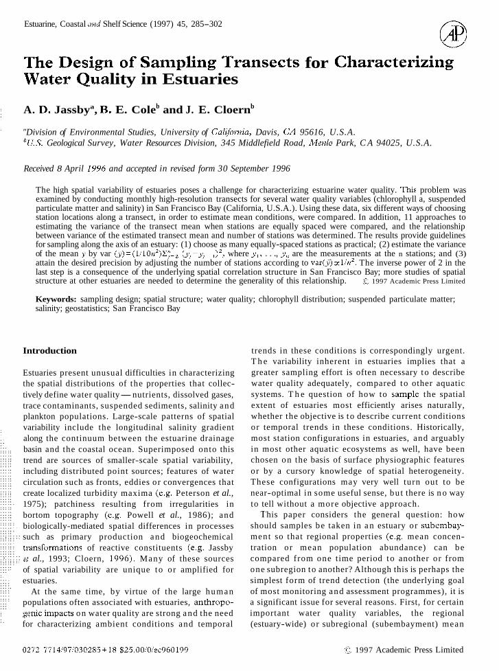
FIGURE 1. San Francisco Bay. 'Ihe MXDAS cruise track is shown as a solid line along the axis of the estuary.

water column proper. The specific goal is to choose a minimal number of sampling locations along the transect from which one can estimate a scalar index of conditions (in this case, the mean) with sufficient precision (i.e. with sufficiently low variance) that useful comparisons can be made among different time periods.

Deciding on a station array requires consideration of three linked issues, addressed here in sequence:

(1) What kind of sampling design should be adopted (e.g. random, systematic or stratified)?

(2) How can the precision (variance) of the transect mean be estimated?

(3 For a prescribed level of precision, how many samples (stations along a transect) are required?

Answers to these questions require knowledge about the underlying distribution of the parent popu-

lation of all possible samples. The authors' approach is empirical and is not driven by theoretical assump- tions about the underlying distribution. Although it is impossible to sample the entire population of water quality measurements in an estuary, a surrogate parent population can be acquired by collecting a large number (thousands) of samples as closely- spaced sensor measurements made while a ship pro- files an axial transect. A modified version of the integrated software-instrument package MIDAS (Multiple Interface Data Acquisition System; Walser et al., 1992; see also Madden & Day, 1992) was used to collect and store measurements from flow-through water quality sensors and a Global Positioning System (GPS) navigation system. Subsampling from the high- resolution MIDAS transect data was then used to address the issues listed above.

288 A. D. Jassby et al.

We begin with a consideration of the spatial Sam- pling design (Issue #I) . In simple random sampling, each station is selected randomly and independently in space along the transect line. Although simple in concept and obviously unbiased, random sampling has an important drawback in situations where the spatial correlation is high; if two stations are randomly chosen too close together, then they will have similar values and one of them is, to a certain extent, wasted.

Systematic sampling, i.e. equidistant spacing of stations along the transect line, avoids this problem and therefore yields a more precise estimate of the spatial mean in many situations (Murthy & Rao, 1988). A more precise estimate of the spatial mean implies, in turn, that temporal trends of a given size can be detected in fewer years or, alternately, that smaller temporal trends can be detected in any given time interval. Systematic spatial designs are also more convenient to implement. Systematic samples suffer, however, from a serious drawback in that unbiased estimates of precision are unavailable, and approximations based on assumptions about the nature of the underlying population must be utilized (Bellhouse, 1988). The precision cannot be estimated based on the sampling design alone because a systematic sample is essentially a random sample of size one; once the first station is selected, the locations of the others are completely specified as well. Furthermore, systematic sampling does not always yield the most precise estimates; the relative performance of different designs depends on the structure of the underlying population (Cochran, 1977).

Stratified sampling refers to, in this case, dividing a relatively heterogeneous estuary into more homo- geneous subdomains and then carrying out either a random or systematic programme of sampling inde- pendently within each subdomain (stratum). Insofar as the within-subdomain variability is reduced relative to the between-subdomain variability, stratification can lead to a more precise estimate of the mean than either simple random or systematic sampling (Cochran, 1977). The strong spatial correlation char- acteristic of estuaries (Powell et al., 1986) suggests that stratification of sampling into spatially contiguous subregions might be appropriate. In order to choose the strata in a consistent way, a novel method is employed here; the machinery of tree-based modelling (Clark & Pregibon, 1992).

The MIDAS transect data enable one to evaluate the relative performance of these different sampling designs. In particular, simple random sampling, sys- tematic sampling and their stratified counterparts,

stratified random and stratified systematic sampling, are compared.

As suggested above, if systematic sampling turns out to give the most precise estimate of the underlying mean, one must decide how the variance of the estimate can best be calculated from the low- resolution station arrays commonly encountered in practice (Issue # 2 ) . Many different estimators have been proposed, most of which are based on an as- sumed model of population behaviour and so are appropriate only when the model truly represents the population. Whether or not a single tractable model can be applied to estuarine data in general is not known. At different times and locations, transects appear to be dominated by noise, linear or higher- order trends, persistence (spatial autocorrelation) or, most often, a complex combination of these basic patterns. When only low-resolution samples are avail- able, there is little hope of identifying a suitable model. The authors' intention is, therefore, to assess the robustness of the different estimators for use when high-resolution data are not accessible, given that the appropriate model may be temporally sensitive. Sub- sets of these methods have been compared for demo- graphic (Wolter, 1984) and stereological (Mattfeldt, 1989) data but their relative performance cannot be extrapolated to natural ecosystems, which can exhibit quite different population structures. Again, the MI- DAS data enable a direct assessment of the different variance estimators by providing high-resolution de- scriptions of the underlying populations in an estuary.

Given a sampling design and a way to estimate the resulting precision, how does one choose an appropri- ate number of stations (Issue #3)? The use of some criterion of performance or objective function is an essential step in completing this phase of design, but the criterion depends on the overall monitoring objective (e.g. to describe ambient conditions, assess compliance with standards, detect trends or determine causal mechanisms) and the costs and uncertainties associated with different designs. Rather than linking this analysis to a specific objective function, it was asked how the ability to reproduce the underlying data, as measured by the variance of the estimated mean, depends on the number of stations. This rela- tion is simple enough to calculate with a high- resolution data set in hand, but of specific interest is what can be said when the only data available are from sparser transects (i.e. the usual kind of data collected in monitoring programmes). Therefore, one should look for generalities in the relation that may be char- acteristic of the underlying spatial structure in an estuary, and can be used to guide sample size when only low-resolution data are available.

Water quality in estuaries 289

Month (water year 1995)

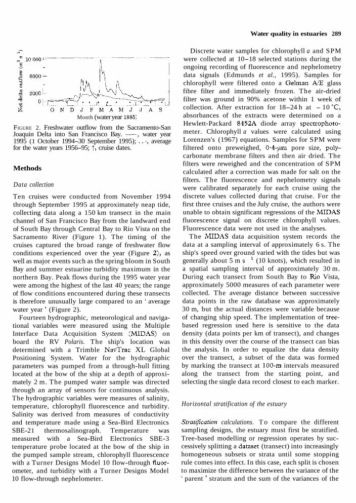
FIGURE 2. Freshwater outflow from the Sacramento-San Joaquin Delta into San Francisco Bay. ---, water year 1995 (1 October 1994-30 September 1995); . . ., average for the water years 1956-95; 1, cruise dates.

Methods

Data collection

Ten cruises were conducted from November 1994 through September 1995 at approximately neap tide, collecting data along a 150 km transect in the main channel of San Francisco Bay from the landward end of South Bay through Central Bay to Rio Vista on the Sacramento River (Figure 1). The timing of the cruises captured the broad range of freshwater flow conditions experienced over the year (Figure 2), as well as major events such as the spring bloom in South Bay and summer estuarine turbidity maximum in the northern Bay. Peak flows during the 1995 water year were among the highest of the last 40 years; the range of flow conditions encountered during these transects is therefore unusually large compared to an ' average water year ' (Figure 2).

Fourteen hydrographic, meteorological and naviga- tional variables were measured using the Multiple Interface Data Acquisition System (MIDAS) on board the RV Polaris. The ship's location was determined with a Trimble NavTrac XL Global Positioning System. Water for the hydrographic parameters was pumped from a through-hull fitting located at the bow of the ship at a depth of approxi- mately 2 m. The pumped water sample was directed through an array of sensors for continuous analysis. The hydrographic variables were measures of salinity, temperature, chlorophyll fluorescence and turbidity. Salinity was derived from measures of conductivity and temperature made using a Sea-Bird Electronics SBE-2 1 thermosalinograph. Temperature was measured with a Sea-Bird Electronics SBE-3 temperature probe located at the bow of the ship in the pumped sample stream, chlorophyll fluorescence with a Turner Designs Model 10 flow-through fluor- ometer, and turbidity with a Turner Designs Model 10 flow-through nephelometer.

Discrete water samples for chlorophyll a and SPM were collected at 10-18 selected stations during the ongoing recording of fluorescence and nephelometry data signals (Edmunds et al., 1995). Samples for chlorophyll were filtered onto a Gelman A/E glass fibre filter and immediately frozen. The air-dried filter was ground in 90% acetone within 1 week of collection. After extraction for 18-24 h at - 10 "C, absorbances of the extracts were determined on a Hewlett-Packard 8452A diode array spectrophoto- meter. Chlorophyll a values were calculated using Lorenzen's (1967) equations. Samples for SPM were filtered onto preweighed, 0.4-pm pore size, poly- carbonate membrane filters and then air dried. The filters were reweighed and the concentration of SPM calculated after a correction was made for salt on the filters. The fluorescence and nephelometry signals were calibrated separately for each cruise using the discrete values collected during that cruise. For the first three cruises and the July cruise, the authors were unable to obtain significant regressions of the MIDAS fluorescence signal on discrete chlorophyll values. Fluorescence data were not used in the analyses.

The MIDAS data acquisition system records the data at a sampling interval of approximately 6 s. The ship's speed over ground varied with the tides but was generally about 5 m s - ' (1 0 knots), which resulted in a spatial sampling interval of approximately 30 m. During each transect from South Bay to Rio Vista, approximately 5000 measures of each parameter were collected. The average distance between successive data points in the raw database was approximately 30 m, but the actual distances were variable because of changing ship speed. The implementation of tree- based regression used here is sensitive to the data density (data points per km of transect), and changes in this density over the course of the transect can bias the analysis. In order to equalize the data density over the transect, a subset of the data was formed by marking the transect at 100-m intervals measured along the transect from the starting point, and selecting the single data record closest to each marker.

Horizontal stratification of the estuary

Strat$cation calculations. T o compare the different sampling designs, the estuary must first be stratified. Tree-based modelling or regression operates by suc- cessively splitting a dataset (transect) into increasingly homogeneous subsets or strata until some stopping rule comes into effect. In this case, each split is chosen to maximize the difference between the variance of the ' parent ' stratum and the sum of the variances of the

290 A. D. Jassby et al.

two ' children ' strata. As different transects and vari- ables result in different splits, a further step is to extract from the combined collection of splits those regions where they tend to cluster and collectively support the placement of a boundary. Tree-based modelling therefore serves more as a guide to the location of strata boundaries rather than an exact specification of these boundaries.

Trees were ' grown ' using the algorithms of S-PLUS (Clark & Pregibon, 1992; Statistical Sciences, 1994). Each transect was successively split along the transect path in order to maximize the quantity AD:

where y, is the ith observation in the parent stratum; ,u is the mean value of the parent stratum; L and R are the sets of indices defining the left-hand and right- hand children strata, respectively; and p, and p, are the mean values in the two respective children strata. The splitting process continued until none of the resulting strata could account for more than 10% of the original variance. Strata were then compared among variables for the same transect and among transects for the same variable. The value of 10% was chosen because smaller values resulted in strata that were probably dependent on tidal stage. For example, the splits computed for two successive transects on 18 and 19 January 1995 (beginning at the same time of day but at opposite ends of the Bay) essentially coincided if 10% was used as a cutoff; on the other hand, splits that resulted in strata accounting for less than 10% of the original variance did not coincide.

Sample allocation among strata. In order to test the efficacy of a stratification scheme, one must also decide how to allocate samples among the various strata. This can be done in several different ways. The simplest method is proportional allocation, in which the number of samples in any stratum is directly propor- tional to the stratum size. Stratum size in the case of a LI/LIDAS transect is simply the length along the transect between stratum boundaries.

In contrast to proportional allocation, the most efficient or optimal allocation of stations among strata takes into account stratum variability and sampling costs, in addition to stratum size. For any stratum i of a transect, the number of stations that minimizes the variance of the estimated mean for a given total cost is:

where W, is the stratum size, S, is the stratum standard deviation and c, is the cost per sample in that stratum (Cochran, 1977). If the cost of sampling a station is constant throughout the estuary, then Equation 2 implies that the density of stations within a stratum is simply proportional to the standard deviation of the transect variable.

Due to the potential discrepancy in optimal alloca- tions for different variables (due to different values of S,), the efficacy of a compromise allocation among strata was also examined. The compromise was effected by minimizing the average over all three variables of the proportional increase in variance over optimal allocation (Chatterjee, 1967). It can be shown that the resulting sample sizes are:

where nii is the optimum sample size in stratum i for variable j.

Sampling design

The variance of the mean was calculated for several different practical sampling strategies, and compared to simple random sampling. The authors' approach was to regard the MIDAS transect data as the under- lying population. The variance of the simple random sampling estimate is then given by:

S2 var (Yran) = ( 1 - f ) -

n (4)

where S is the population standard deviation, n is the sample size, and f=n/N is the sampling fraction with N the population size (Cochran, 1977). In practice, n will be much less than 75 and N is usually around 1500, so the true sampling fraction is much less than 5%. As a rule of thumb, the finite population correction (1-fl can be ignored when f<0.05 (Barnett, 1991), and it will be ignored in what follows.

For stratified random sampling, the variance of the estimated mean depends on the sample allocation strategy. In the case of proportional allocation, the variance is:

1 var (y,,) = - W, S,Z

n,=1 (5)

where W, is the relative size and S, is the standard deviation of the ith stratum, and there are h strata. For optimal allocation, the corresponding calculation is:

Water quality in estuaries 291

The variance for a compromise allocation can be determined from the general result for stratified samples, which can be expressed in the form:

1 W?S? var (y,,) = - C -

n i , l ri

where nj=nai. The traditional station configuration in San

Francisco Bay has been an approximately systematic one, i.e, with equal distances between adjacent stations. Assuming AT is a multiple of n, there are m=Mn possible systematic samples. When AT was not a multiple, the method of circular systematic sampling due to Lahiri (Bellhouse, 1988) was used. The variance of the systematic estimate is then simply:

where Pk is the mean of the kth potential systematic sample and p i s the transect mean.

Finally, the performance of stratified sampling with proportional allocation was investigated again, but with systematic rather than simple random sampling within strata. Variances within strata are then given by Equation 8, but the variance of the estimated overall transect mean is:

var (g,,,) = C Wz var (Ji) i = 1

(9)

where varGi) is the variance for the estimated mean of stratum z.

Each sampling strategy was compared to simple random sampling by calculating the percent decrease in variance 100(1 - VIVr,,), where Vpa, is the variance given by Equation 4 and V is the variance due to one of the other strategies. For stratified random sampling, n drops out and the comparisons are independent of sample size. For systematic and strati- fied systematic, however, the ratio depends on n and so the results for three sample sizes (10, 20 and 40), typical of the range for transects in estuarine research and monitoring programmes and specifically covering the range used in San Francisco Bay, were examined.

Variance estimators

A variety of estimators that have been proposed for systematic sampling and that are simple to compute

were examined (Table 1). The first estimator SRS is simply the variance of the simple random sampling estimate (Equation 4). Estimator MURTl considers the systematic sample as a stratified random sample with two samples from each of nl2 strata; MURT2 is similar but based on successive differences (Murthy & Rao, 1988). The next three estimators are based on higher-order differences; WOLTl and WOLT2 attempt to account for trends and WOLT3 for auto- correlation (Wolter, 1984). The estimator KOOP consists of a pseudo-replication in which the sample is split into two systematic subsamples (Koop, 1971). The next three estimators also attempt to take into account the spatial correlation structure of the popu- lation. Estimator COCH is an asymptotic result due to Cockran (1 946) and assumes an autoregressive pro- cess of order one; estimators CHEV (Yates, 1960; Chevrou, 1976) and GUND (Gunderson & Jensen, 1987) are based on regionalized variable theory (Mattfeldt, 1989). CHEV was developed specifically for error estimation in linear systematic arrays, while GUND is based on a quadratic approximation to the variogram. The final estimator MAHA is based on two independent systematic samples of size nl2, a technique known as the method of interpenetrating subsamples (Mahalanobis, 1946).

The estimators for sample sizes of 10, 20 and 40 stations were compared. For a given sample size, hydrographic variable and transect, each estimator was applied to all possible systematic samples, and the performance of an estimator was summarized with the mean square error MSE:

Results for all transects, for a given sample size and variable, were then averaged and ranked.

Sample size

The relation between variance and sample size was demonstrated empirically by computing varG) (Equa- tion 8) from all possible systematic subsamples for a range of sample sizes, specifically 5 through 50. This range encompasses the number of fixed stations likely to be encountered in practice. The calculation was repeated for each transect and variable. The relation was assumed to be of the form:

and estimates of a were extracted using the Golub- Pereyra algorithm for partially linear models (Bates & Chambers, 1992).

292 A. D. Jassby et al.

TABLE 1. Estimators of variance for systematic sampling

Estimator Description

1 SRS s2/n, where s2 = ZJ=, (yj-9) '/(n - 1)

2 MURTl (l/n)Zy!!,aij/n, where aj=yi-yj_,

3 MURT2 (lln)Z:_,a:/2(n- I ) , where a j = y j - y J l

4 WOLTl (l/n)ZJ=,bf/6(n-2), where bj=yj-2yj-1+yj-2

5 WOLT2 (l/n)Zl=,c:/3.5(n-4), where cj=yj/2 -yj-, +yj-, -yj_, +yj-4/2

6 WOLT3 (l/n)X~=,d:/7.5(n- 8), where dj=yj/2-yj- +. . . -31 j - , f yj-,/2

7 KOOP (114) {(21n)Zj eve,,yj- (2172) Ej oddyj)2

8COCH (s2/n)(1+(2flnp)+2/(p-1-1)~,wherep=C~=,(y-~)(yi-l-~)/{s2(n-1))

9 CHEV (l/n)X~=,a~/lOn, where aj=yjPyj-

10 GUND ( l / n ) {3CS=,y~+X~=3y jy j -2 -4Z~="=, j y j - l ) / 12

11 MAHA (112) X:=, ( j j i -9) 2, where Yi are means of independent samples of size n/2

The sample is denoted by y,, j = 1,2, . . . ,n.

The relation between variance and sample size is also a relation between variance and interstation distance. In order to portray how variance changes with spatial scale, as opposed to sample size, var(9) (Equation 8) was computed from all possible systematic subsamples for station separations of 1-64 km.

Results

Horizontal strat$cation of the estua y

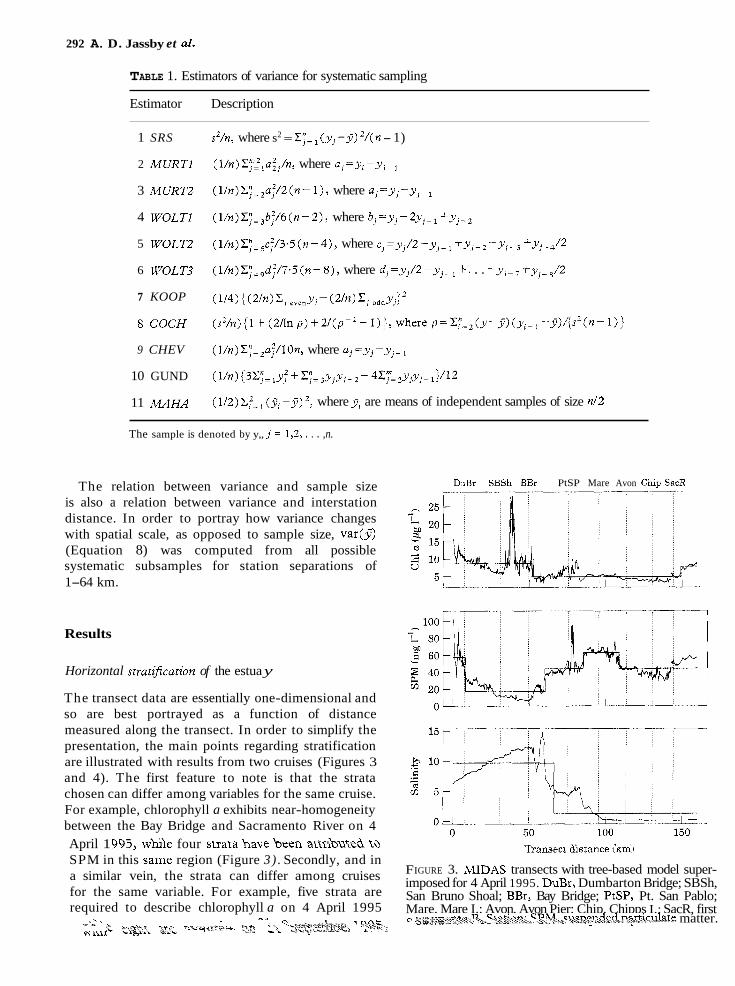
The transect data are essentially one-dimensional and so are best portrayed as a function of distance measured along the transect. In order to simplify the presentation, the main points regarding stratification are illustrated with results from two cruises (Figures 3 and 4). The first feature to note is that the strata chosen can differ among variables for the same cruise. For example, chlorophyll a exhibits near-homogeneity between the Bay Bridge and Sacramento River on 4 April 1 995, n ~ ~ ) e four srrata ha\; e bcm ; h i ' i ~ h t & to SPM in this same region (Figure 3) . Secondly, and in a similar vein, the strata can differ among cruises for the same variable. For example, five strata are required to describe chlorophyll a on 4 April 1995

\' \ -" ~ - " -.

* ,ii, T - y L -"J="=" C F -b 'll y-%m.- 1111:1, \ :?i? -Lq3q-+~2>k> ' ?SF._

D J B ~ SBSh BBr PtSP Mare Avon C h ~ p SacR -------

FIGURE 3. MIDAS transects with tree-based model super- imposed for 4 April 1995. DuBr, Dumbarton Bridge; SBSh, San Bruno Shoal; BBr, Bay Bridge; PtSP, Pt. San Pablo; Mare, Mare I.; Avon, Avon Pier; Chip, Chipps I.; SacR, first P . ~ E , ~ ~ ~ ~ ~ ~ ~ ~ ~ ~ r \ . ~ ~ ~ ~ ~ P ~ ~ $ . C ~ ~ ~ ~ ~ ~ ~ ~ ~ ~ n ~ ~ i c ~ ~ b t e -..- matter.

Water quality in estuaries 293

DuBr SBSh BBr PtSP Mare Avon C h ~ p SacR - - --

0 50 100 150 Transect distance (km)

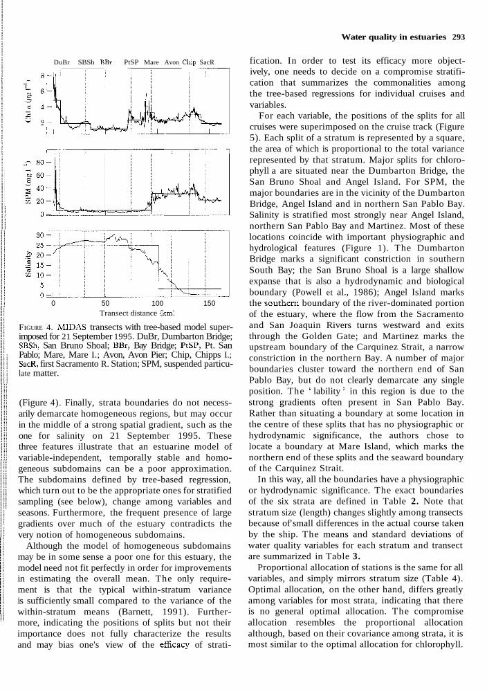
FIGURE 4. MIDAS transects with tree-based model super- imposed for 21 September 1995. DuBr, Dumbarton Bridge; SBSh, San Bruno Shoal; BBr, Bay Bridge; PtSP, Pt. San Pablo; Mare, Mare I.; Avon, Avon Pier; Chip, Chipps I.; SacR, first Sacramento R. Station; SPM, suspended particu- late matter.

(Figure 4). Finally, strata boundaries do not necess- arily demarcate homogeneous regions, but may occur in the middle of a strong spatial gradient, such as the one for salinity on 21 September 1995. These three features illustrate that an estuarine model of variable-independent, temporally stable and homo- geneous subdomains can be a poor approximation. The subdomains defined by tree-based regression, which turn out to be the appropriate ones for stratified sampling (see below), change among variables and seasons. Furthermore, the frequent presence of large gradients over much of the estuary contradicts the very notion of homogeneous subdomains.

Although the model of homogeneous subdomains may be in some sense a poor one for this estuary, the model need not fit perfectly in order for improvements in estimating the overall mean. The only require- ment is that the typical within-stratum variance is sufficiently small compared to the variance of the within-stratum means (Barnett, 1991). Further- more, indicating the positions of splits but not their importance does not fully characterize the results and may bias one's view of the efficacy of strati-

fication. In order to test its efficacy more object- ively, one needs to decide on a compromise stratifi- cation that summarizes the commonalities among the tree-based regressions for individual cruises and variables.

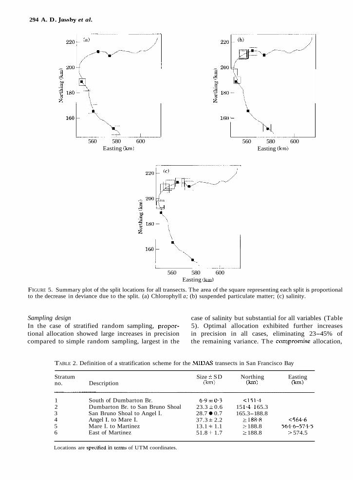
For each variable, the positions of the splits for all cruises were superimposed on the cruise track (Figure 5). Each split of a stratum is represented by a square, the area of which is proportional to the total variance represented by that stratum. Major splits for chloro- phyll a are situated near the Dumbarton Bridge, the San Bruno Shoal and Angel Island. For SPM, the major boundaries are in the vicinity of the Dumbarton Bridge, Angel Island and in northern San Pablo Bay. Salinity is stratified most strongly near Angel Island, northern San Pablo Bay and Martinez. Most of these locations coincide with important physiographic and hydrological features (Figure 1). The Dumbarton Bridge marks a significant constriction in southern South Bay; the San Bruno Shoal is a large shallow expanse that is also a hydrodynamic and biological boundary (Powell et al., 1986); Angel Island marks the southern boundary of the river-dominated portion of the estuary, where the flow from the Sacramento and San Joaquin Rivers turns westward and exits through the Golden Gate; and Martinez marks the upstream boundary of the Carquinez Strait, a narrow constriction in the northern Bay. A number of major boundaries cluster toward the northern end of San Pablo Bay, but do not clearly demarcate any single position. The ' lability ' in this region is due to the strong gradients often present in San Pablo Bay. Rather than situating a boundary at some location in the centre of these splits that has no physiographic or hydrodynamic significance, the authors chose to locate a boundary at Mare Island, which marks the northern end of these splits and the seaward boundary of the Carquinez Strait.

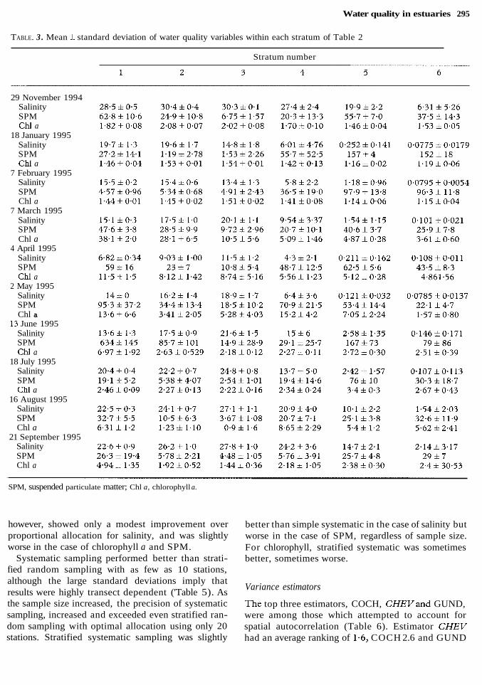
In this way, all the boundaries have a physiographic or hydrodynamic significance. The exact boundaries of the six strata are defined in Table 2. Note that stratum size (length) changes slightly among transects because of' small differences in the actual course taken by the ship. The means and standard deviations of water quality variables for each stratum and transect are summarized in Table 3.

Proportional allocation of stations is the same for all variables, and simply mirrors stratum size (Table 4). Optimal allocation, on the other hand, differs greatly among variables for most strata, indicating that there is no general optimal allocation. The compromise allocation resembles the proportional allocation although, based on their covariance among strata, it is most similar to the optimal allocation for chlorophyll.

294 A. D. Jassby et al.

560 580 600 Easting (km)

L U __---.. 1 -.------.. 560 580 600

Easting (km)

560 580 600 Easting (km)

FIGURE 5. Summary plot of the split locations for all transects. The area of the square representing each split is proportional to the decrease in deviance due to the split. (a) Chlorophyll a; (b) suspended particulate matter; (c) salinity.

Sampling design case of salinity but substantial for all variables (Table In the case of stratified random sampling, propor- 5). Optimal allocation exhibited further increases tional allocation showed large increases in precision in precision in all cases, eliminating 23-45% of compared to simple random sampling, largest in the the remaining variance. The compromise allocation,

TABLE 2. Definition of a stratification scheme for the MIDAS transects in San Francisco Bay

Stratum Size f SD Northing Easting no. Description (km) (km) (km)

1 South of Dumbarton Br. 6.9 * 0.3 <151.4 2 Dumbarton Br. to San Bruno Shoal 23.3 & 0.6 15 1.4-1 65.3 3 San Bruno Shoal to Angel I. 28.7 0.7 165.3-1 88.8 4 Angel I. to Mare I. 37.3 f 2.2 2 188.8 <564.6 5 Mare I. to Martinez 13.1 5 1.1 > 188.8 564.6-574.5 6 East of Martinez 51.8 & 1.7 > 188.8 2 574.5

Locations are specified in ternis of UTM coordinates.

Water quality in estuaries 295

TABLE. 3 . Mean f standard deviation of water quality variables within each stratum of Table 2

Stratum number

29 November 1994 Salinity SPM Chl a

18 January 1995 Salinity SPM Chl a

7 February 1995 Salinity SPM Chl a

7 March 1995 Salinity SPM Chl a

4 April 1995 Salinity SPM Chl a

2 May 1995 Salinity SPM Chl a

13 June 1995 Salinity SPM Chl a

18 July 1995 Salinity SPM Chl a

16 August 1995 Salinity SPM Chl a

21 September 1995 Salinity SPM Chl a

SPM, suspended particulate matter; Chl a, chlorophyll a.

however, showed only a modest improvement over proportional allocation for salinity, and was slightly worse in the case of chlorophyll a and SPM.

Systematic sampling performed better than strati- fied random sampling with as few as 10 stations, although the large standard deviations imply that results were highly transect dependent ('Table 5). As the sample size increased, the precision of systematic sampling, increased and exceeded even stratified ran- dom sampling with optimal allocation using only 20 stations. Stratified systematic sampling was slightly

better than simple systematic in the case of salinity but worse in the case of SPM, regardless of sample size. For chlorophyll, stratified systematic was sometimes better, sometimes worse.

Variance estimators

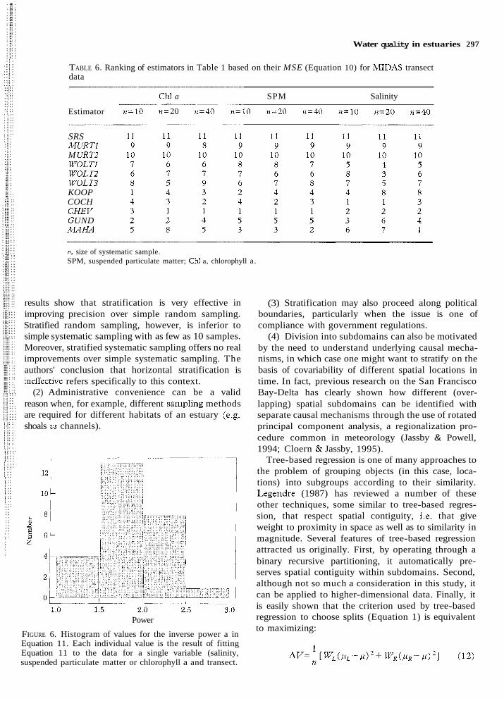
?'he top three estimators, COCH, CHEVand GUND, were among those which attempted to account for spatial autocorrelation (Table 6). Estimator CHEV had an average ranking of 1.6, COCH 2.6 and GUND

296 A. D. Jassby et al.

TABLE 4. Sample sizes within strata expressed as a percentage of the total number of samples

Optimal Allocation I SL) Stratum Proport~onal - - ~

no. allocation i SD Chlorophyll a SPM Salin~ty Compromise

allocation f SD

SPM, suspended particulate matter. The standard deviations represent variation among transects.

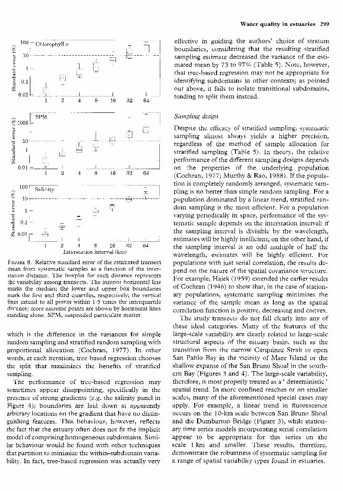
4.0. The next best estimators were KOOP and The relative standard error of the median transect is MAHA, which base their estimates on two subsamples almost always less than 10% when stations are spaced of equal size. The estimator SRS, which treats the up to 8 km apart (Figure 8). sample as if it were a simple random sample, is highly inefficient; it came in last in every instance.

Discussion

Sample size

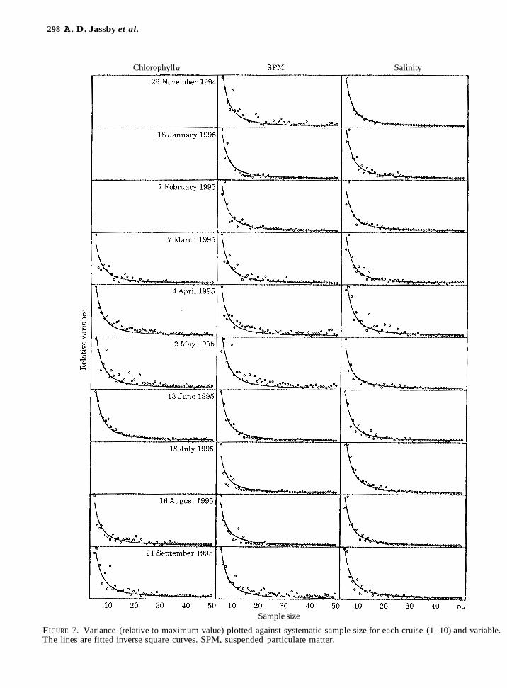
Fits of the inverse power relationship separately to each variable and transect (Equation 11) resulted in a narrow range of a averaging 1.9 ic 0.1 (SE) (Figure 6). No significant effects of either variables or transects were found. For theoretical reasons discussed below, the ability of an inverse square curve to fit all data simultaneously was examined. The resulting fits each appeared to be a satisfactory description of the data (Figure 7).

Horizontal stratification of the estua y

Horizontal stratification of an estuary, i.e. division of the estuary into subdomains, can be motivated by many difTerent goals:

(1) The need for precise estimates of estuary-wide statistics such as the overall mean was the authors' primary motivation. As discussed above, if the estuary can be divided into subdomains that are relatively homogeneous compared to the between-subdomain variability, then estimates of the overall mean will be more precise than for a simple random sample. These

TABLE 5 . Percent decrease in var(j) compared to simple random sampling for different types of sampling strategies

Sampling type Chlorophyll a k SD SPM SD Salinity + SD

Stratified random Proportional Optimal Compromise

n= 10 Systematic Stratified systematic

n=20 Systematic Stratified systematic

n=40 Systematic Stratified systematic

SPM, suspended particulate matter. The standard devlanons represent variation among transects.

Water quality in estuaries 297

TABLE 6. Ranking of estimators in Table 1 based on their MSE (Equation 10) for MIDAS transect data

Chl a SPM Salinity - -.

Estimator n=10 n=20 n=40 n=10 n=20 n=40 n=10 n=20 n=40

SRS MURTl M UR T2 WOLTl WOLT2 WOL'13 KOOP COCH CHEV G UND MAHA

n, size of systematic sample. SPM, suspended particulate matter; Chl a, chlorophyll a.

results show that stratification is very effective in improving precision over simple random sampling. Stratified random sampling, however, is inferior to simple systematic sampling with as few as 10 samples. Moreover, stratified systematic sampling offers no real improvements over simple systematic sampling. The authors' conclusion that horizontal stratification is ineffective refers specifically to this context.

(2) Administrative convenience can be a valid reason when, for example, different sampling methods are required for different habitats of an estuary (e.g. shoals us channels).

Power

FIGURE 6. Histogram of values for the inverse power a in Equation 11. Each individual value is the result of fitting Equation 11 to the data for a single variable (salinity, suspended particulate matter or chlorophyll a and transect.

(3) Stratification may also proceed along political boundaries, particularly when the issue is one of compliance with government regulations.

(4) Division into subdomains can also be motivated by the need to understand underlying causal mecha- nisms, in which case one might want to stratify on the basis of covariability of different spatial locations in time. In fact, previous research on the San Francisco Bay-Delta has clearly shown how different (over- lapping) spatial subdomains can be identified with separate causal mechanisms through the use of rotated principal component analysis, a regionalization pro- cedure common in meteorology (Jassby & Powell, 1994; Cloern & Jassby, 1995).

Tree-based regression is one of many approaches to the problem of grouping objects (in this case, loca- tions) into subgroups according to their similarity. Legendre (1987) has reviewed a number of these other techniques, some similar to tree-based regres- sion, that respect spatial contiguity, i.e. that give weight to proximity in space as well as to similarity in magnitude. Several features of tree-based regression attracted us originally. First, by operating through a binary recursive partitioning, it automatically pre- serves spatial contiguity within subdomains. Second, although not so much a consideration in this study, it can be applied to higher-dimensional data. Finally, it is easily shown that the criterion used by tree-based regression to choose splits (Equation 1) is equivalent to maximizing:

298 A. D. Jassby et al.

Chlorophyll a SPM Salinity

Sample size

FIGURE 7. Variance (relative to maximum value) plotted against systematic sample size for each cruise (1-10) and variable. The lines are fitted inverse square curves. SPM, suspended particulate matter.

Water quality in estuaries 299

1 2 4 8 16 32 64 Interstation interval (km)

FIGURE 8. Relative standard error of the estimated transect mean from systematic samples as a function of the inter- station distance. The boxplot for each distance represents the variability among transects. The interior horizontal line marks the median; the lower and upper box boundaries mark the first and third quartiles, respectively; the vertical lines extend to all points within 1.5 times the interquartile distance; more extreme points are shown by horizontal lines standing alone. SPM, suspended particulate matter.

which is the difference in the variances for simple random sampling and stratified random sampling with proportional allocation (Cochran, 1977). In other words, at each iteration, tree-based regression chooses the split that niaxiniizes the benefits of stratified sampling.

The performance of tree-based regression may sometimes appear disappointing, specifically in the presence of strong gradients (e.g. the salinity panel in Figure 4); boundaries are laid down at apparently arbitrary locations on the gradient that have no distin- guishing features. This behaviour, however, reflects the fact that the estuary often does not fit the implicit model of comprising homogeneous subdomains. Simi- lar behaviour would be found with other techniques that partition to minimize the within-subdomain varia- bility. In fact, tree-based regression was actually very

effective in guiding the authors' choice of stratum boundaries, considering that the resulting stratified sampling estimate decreased the variance of the esti- mated mean by 73 to 97% (Table 5). Note, however, that tree-based regression may not be appropriate for identifying subdomains in other contexts; as pointed out above, it fails to isolate transitional subdomains, tending to split them instead.

Sampling design

Despite the efficacy of stratified sampling, systematic sampling almost always yields a higher precision, regardless of the method of sample allocation for stratified sampling (Table 5). In theory, the relative performance of the different sampling designs depends on the properties of the underlying population (Cochran, 1977; Murthy & Rao, 1988). If the popula- tion is completely randomly arranged, systematic sam- pling is no better than simple random sampling. For a population dominated by a linear trend, stratified ran- dom sampling is the most efficient. For a population varying periodically in space, performance of the sys- tematic sample depends on the interstation interval: if the sampling interval is divisible by the wavelength, estimates will be highly inefficient; on the other hand, if the sampling interval is an odd multiple of half the wavelength, estimates will be highly efficient. For populations with just serial correlation, the results de- pend on the nature of the spatial covariance structure. For example, Hajek (1959) extended the earlier results of Cochran (1946) to show that, in the case of station- ary populations, systematic sampling minimizes the variance of the sample mean as long as the spatial correlation function is positive, decreasing and convex.

'l'he study transects do not fall clearly into any of these ideal categories. Many of the features of the large-scale variability are clearly related to large-scale structural aspects of the estuary basin, such as the transition from the narrow Carquinez Strait to open San Pablo Bay in the vicinity of Mare Island or the shallow expanse of the San Bruno Shoal in the south- ern Bay (Figures 3 and 4). The large-scale variability, therefore, is most properly treated as a ' deterministic ' spatial trend. In more confined reaches or on snialler scales, many of the aforementioned special cases may apply. For example, a linear trend in fluorescence occurs on the 10-km scale between San Bruno Shoal and the Dumbarton Bridge (Figure 3), while station- ary time series models incorporating serial correlation appear to be appropriate for this series on the scale 1 km and smaller. These results, therefore, demonstrate the robustness of systematic sampling for a range of spatial variability types found in estuaries.

300 A. D. Jassby et al.

Note that a stratified systematic design offers only modest improvements at best, and sometimes even worse precision than unstratified systematic sampling (Table 5). As the systematic samples for different strata are chosen independently, stations from differ- ent strata may fall very close together near boundaries between strata and provide redundant information, also a failing of both the simple and stratified random design. The improvements are too modest to warrant the additional complications of stratified systematic sampling.

Variance estimators

The variance estimators with the lowest MSE (Equa- tion 10)-COCH, CHEV and GUNS --a re those specifically devised to account for spatial autocorrela- tion in the population (Table 1). Estimator CHEV is recommended on the basis of its empirical perfonn- ance; interestingly, it was designed specifically for linear systematic samples (Chevrou, 1976) and the results here attest to the success of that design. Esti- mator COCH would also be a good choice. It is one devised by Cochran (1 946) for stationary populations with an autoregressive structure of order one, equiva- lent to an exponential correlogram or variogram. As discussed below, the correlograms commonly encoun- tered in these data are in fact exponential. Wolter (1 984) observed that this estimator had remarkably good properties for artificial populations that are dominated by linear trends or autocorrelation. On the other hand, it was found that treating the systematic sample as if it were a simple random sample (SRS) leads to a poor estimate of the variance. Note also that MURTI and MURT2 turned out to be relatively inefficient for these estuarine data, in contrast to their superior performance for demographic data (Wolter, 1984).

Sample size

The relation between variance of the mean and sample size is well described by an inverse power law with an average power of 1.9 i 0.1 and more than 80% of the cases occur in the range 1.5-2.5 (Figure 6). It can be shown that the power is related to the nature of the variogram (Simard et al., 1992). Let n systematic samples be taken along the transect dis- tance T, so L=Tln is the distance between samples. Suppose for distances h up to L, the variogram has the fonn:

y(h) = chb, with 0 2 b < 2

where c is a constant. Then one can derive for the one-dimensional case (namely, a transect) that (L).

Marcotte, pers. comm.):

Now in the case of exponential, linear or spherical variograms (Isaaks & Srivastava, 1989), provided that the range is much larger than L, b = 1 and an inverse square law would be expected. For Gaussian vario- grams, which have parabolic as opposed to linear behaviour near the origin, b=2, and for a nugget effect, b=O, so that a different power law would hold in these cases. The present finding of an inverse square law is therefore in agreement with past studies of spatial correlation in San Francisco Bay, which have demonstrated the presence of exponential spatial correlation (Powell et al., 1 986).

How widely can the inverse square relationship be applied to other systems? Based on the above argu- ments, this question can be rephrased by asking how representative are variograms with linear behaviour near the origin (i.e. linear, exponential and spherical variograms). A nugget effect has been observed for water quality variables in both estuarine (Legendre & Trousellier, 1988; Legendre et al., 1989; S h a r d et al., 1992) and coastal waters (Denman & Freeland, 1985; Yoder et al., 1987). The shapes of the variograms, however, were usually exponential or at least compat- ible with an exponential shape where the resolution was too poor to be certain. Furthermore, the nugget effect may represent sampling error and not be an inherent feature such as high short scale variability (Isaaks & Srivastava, 1989); with more precise measurement techniques, the nugget effect could weaken or disappear. Nonetheless, the evidence from estuaries on variogram shape is sparse. Parabolic behaviour has been observed, moreover, in at least one other tidal estuary; North Inlet, South Carolina (Childers et al., 1994). Based on the existing evidence, an inverse square law cannot therefore be assumed for other estuaries, and the actual power could lie between 1 and 3. There is clearly a need here for expanding the empirical knowledge of estuarine spatial autocorrelation. Theoretical investigation of the link between the variogram or correlogram and underlying physical and biological processes could also help resolve the generality of any sampling design.

Where high-resolution data such as the MIDAS data are not available, it may be possible to take a geostatistical approach both to the variance estimate and the relation between precision and sample size. Based on a model of the underlying spatial auto- correlation, i.e. the variogram, kriging methodology

Water quality in estuaries 301

The r e s u h of this - I UJJ- ~~ ivv lde guidelmes for esti- mating esruaty-:*.I& means with low-resolution data from fixed staiiurl,. C,,en ally desired precision for the estmiate, rli, f i , . ~ s i q ~ is to take systematic

samples with LS rllxlly k t ~ t l o r ~ \ as practical. Next, the estmiator CHEV or COCH (T'able 1) is used to calculate the vallarlce of cach sample, whlch wll of course vary sumewhat from trdnsect LO transect even when the nlmiber of stations IS constant (Flgure 8). Finally, the desiled station number 1s deter~iuned from the typical or characteristic variance found in the prevlous step, the target variance, and the inverse power relation between variance and sample slze. At present, the acrual vaiue for the power must come from prlor knowledge ofrhe variogram or cor~elogram shape or, d enough stations are used, by calculating the varlogralii from the initla1 array of stations. Fur- ther research may reveal some general rules for deduc-

ing variogram shape or this power from features of estuarine dynamics that can be observed with fewer stations.

Acknowledgements

'l'he authors thank Jody Edmunds and Jane Caffrcy for their central roles in the MIDAS data collection effort. Denis Marcotte provided invaluable advice on how spatial structure affects the relationship between variance and saiiiple size; the authors are grateful to him for always being willing to help in a timely fashion and to share his unpublished resulrs. Two anonymous reviewers suggested important improvements to the original manuscript. The data collection and analysis were supported by the San Francisco Estuary Regional Monitoring Program for Trace Substances (SFEI 135-95), the U.S. Geological Survey San Francisco Bay Ecosystem Program and the U.S. Environmental Protection Agency (R8 19658) through the Center for Ecological Health Research at the University of California, Davis. Although the U.S. EPA partially funded preparation of this document, it does not necessarily ref ect the views of the agency and no official endorsement should be inferred.

Keferences

Barnett, V. 199 1 Sairlple Szr~-z.ej~: P~-znriples and Merhods, Edward Arnold, London, 173 pp.

Bates, D. M. & Chambers, J. M. 1992 Nonlinear models. In Statistical Mode1.s in S (Chambers, J. M. & Hastie, T. J., eds). Wadsworth & Brooks;Cole Advanced Books & Software, Pacific Grove, Califorma, pp. 421-454.

Bellhouse, D. R. 1988 Systematic sampling. In Handbook of Sratis- tics, vol. 6 (IG-ishnaiah, P. R. 8r Rao, C. R., eds). Elsevier Science Publishers, Amsterdam, pp. 125-145.

Burgess, I'. M., Webstcr, K. & McBratney, 4 . B. 1981 Optimal inteipolation and isarithmic mapping of soil properties. lV. Sampling strategy. Jozrnzal o f Soil Science 32, 643-659.

Chatterjee, S. 1967 -A note on optimum strarificat~on. Skandinavisk Aktuaneridskr-ift 50, 40-44.

Chevrou, R. B. 1976 PrGcisions des mesures de superficie estimee par grille de points ou intersections de paralleles. Annales des Sciences Fowstiera 33, 257-269.

Childers, D. L., Sklar, F. H . & Hutchinson, S. E. 1994 Staiistical treatment and comparative analysis of scale-dependent aquatic transect data in estuarine landscapes. Landscape Ecology 9, 127- 141.

Clark, L. A. 8r Pregibon, D. 1992 'l'ree-based models. In Statistical Models in S (Chambers, J . M. & Hastie, T. J., eds). Wadswotth & Brooksicole Advanced Books & Soflware, Pacific Grove, California, pp. 37 7-4 1 9.

Cloern, J. E. 1996 Phytoplankton bloom dynamics in coastal ecosystems a review with some general lessons from sustained investigation of San Francisco Bay (California, USA). Rei'iezos of Geophysics 34, 127-168.

Cloern, J. E. & Jassby, A. D. 1995 Year-to-year fluctuation of thc spring phytoplankton bloom in South San Francisco Bay: an example of ecological variabiliiy at the land-sea interface. In Ecological 'fi'nze Sen'es (Steele, J. H . & Powell, T. M., eds). Chapman and Hall, New York, pp. 139-149.

302 A. D. Jassby et al.

Cloern, J. E. & Nichols, F . H. 1985 Temporal dynamics of an estuary: San Francisco Bay. Hydrobiologia 129, 1-237.

Cochran, W. G. 1946 Relative accuracy of systematic and stratified random samples for a certain class of populations. Annals of Mathematical Statistics 17, 164-1 77.

Cochran W. G. 1977 Sampling Techniques, 3rd ed. John Wiley & Sons, New York, 428 pp.

Davis J. A., Gunther, A. J., Richardson, B. J., O'Connor, J. M., Spies, R. B., Wyatt, E., Larson, E. and A. Chan Meiorin. 1991 Status and Trends Report on Pollutants in the Sun Francisco Estua y. San Francisco Estuary Project, Oakland, California, 240 pp.

Denman, K. L. & Freeland, H. J. 1985 Correlation scales, objective mapping and a statistical test of geostrophy over the continental shelf. Journal of Marine Research 43, 5 17-539.

Edmunds J. L., Cole, B. E., Cloern, J. E., Caffrey, J. M. & Jassby, A. D. 1995 Studies ofthe Sun Francisco Bay, California, Estuarine Ecosystem: Pilot Regional Monitoring Results, 1994. Open-File Report 95-378. U.S. Geological Survey, Menlo Park, California, 436 pp.

Gunderson, H . J. G. & Jensen, E. B. 1987 The efficiency of systematic sampling in stereology and its prediction. Journal of Microscopv 147, 229-263.

HBjek, J. 1959 Optimum strategy and other problems in probability sampling. Casopis Pro Pestovani Matematiky 84, 387-420.

Huzzey, L. M., Cloern, J. E. & Powell, T . M. 1990 Episodic changes in lateral transport and phytoplankton distribution in south San Francisco Bay. Limnology and Oceanography 35, 472-478.

Isaaks, E. H. & Srivastava, R. M. . 1989 An Introduction to Applied Geostatisrics. Oxford University Press, New York.

Jassby, A. D. & Powell, T . ,?/I. 1994 Hydrodynamic influences on interannual chlorophyll variability in an estuary: upper San Francisco Bay-Delta (California, U.S.A.). Estuarine, Coastal and Shelf Science 39, 595-6 18.

Jassby, A. D., Cloern, J. E. & Powell, T. M. 1993 Organic carbon sources and sinks in San Francisco Bay: variability induced by river flow. Marine Ecology Progress Series 95, 39-54.

Jassby, A. D., Cloern, J. E., Caffrey, J. M., Cole, B. E. & Rudek, J. 1994 San Francisco BayIDelta Regional Monitoring Program: plankton and water quality pilot study 1993. In San Francisco Estua~l Regional Monitoring Program for Trace Substances: 1993 Annual Report. San Francisco Estuary Institute, Richmond, California, pp. 117-128.

Jassby, A. D., Kimmerer, W. J., Monismith, S. G. et al. 1995 Isohaline position as a habitat indicator for estuarine populations. Ecological Applications 5, 272-289.

Koop, J. C. 1971 On splitting a systematic sample for variance estimation. Annals ofMathematica1 Statistics 42, 1084-1087.

Legendre, P. 1987 Constrained clustering. In Developments in Numerical Ecology (Legendre, P. & Legendre, L., eds). Springer- Verlag, Berlin, pp. 289-307.

Legendre, P. & Troussellier, M. 1988 Aquatic heterotrophic bacteria: Modeling in the presence of spatial autocorrelation. Limnolog\, and Oceanography 33, 1055-1067.

Legendre, P., 'I'roussellier, M., Jarry, V. & Fortin, M.-J. F. 1989 Design for simultaneous sampling of ecological variables: from concepts to numerical solutions. Oikos 55, 3 0 4 2 .

Lorenzen, C. J. 1967 Determination of chlorophyll and pheo- pigments: Spectrophotometric equations. Limno1og)r and Ocea- nography 12, 343-346.

Madden, C. J. & Day, J. W. Jr. 1992 An instrument system for high speed mapping of chlorophyll a and physico-chemical variables in surface waters. Estuaries 15, 421-427.

Mahalanobis, P. C. 1946 Recent experiments in statistical sampling in the Indian Statistical Institute. Journal of the Royal Statistical Society, Series A 109, 325-370.

Mattfeldt, '1'. 1989 The accuracy of one-dimensional systematic sampling. Journal of Microscopy 153, 301-3 13.

Murthy, M. N. & Rao, T. J. 1988 Systematic sampling with illustrative examples. In Handbook ofStatistics, vol. 6 (Krishnaiah, P. R. & Rao, C. R., eds). Elsevier Science, Amsterdam, pp. 147- 185.

Oliver, M. A. & Webster, R. 1991 How geostatistics can help you. Soil Use and Management 7, 206-217.

Peterson, D. H., Conomos, T . J., Broenkow, W. W. & Doherty, P. C. 1975 Location of the non-tidal current null zone in northern San Francsico Bay. Estuarine and Coastal Marine Science 3, 1-11.

Powell, .I'. M., Cloern, J. E. & Walters, R. A. 1986 Phytoplankton spatial distribution in South San Francisco Bay: mesoscale and small-scale variability. In Estuarine Variability (Wolfe, D. A., ed.). Academic Press, London, pp. 369-383.

Powell, T. M., Cloem, J. E. & Huzzey, L. iM. 1989 Spatial and temporal variability in South San Francisco Bay (USA). I. Horizontal distributions of salinity, suspended sediments, and phytoplankton biomass and productivity. Estuarine, Coastal and Shelf Science 28, 583-597.

Rossi, R. E., Mulla, D. J., Journel, A. G. & Franz, E. H. 1992 Geostatistical tools for modeling and interpreting ecological spatial dependence. Ecological Monograplu 62, 277-314.

Simard, Y., Legendre, P. & Lavoie, G. M. D. 1992 Mapping, estimating biomass, and optimizing sampling programs for spa- tially autocorrelated data: case study of the northern shrimp (Pandalus borealis). Canadian Journal of Fisheries and Aquatic Sciences 49, 3 2-4 5.

Statistical Sciences 1995 S-PLUS, Version 3.3for Windows. Statisti- cal Sciences, Seattle, Washington.

'Thioulouse, J., Royet, J. P., Ploye, H. & Houllier, F. 1993 Evalu- ation of the precision of systematic sampling: nugget effect and covariogram modelling. Journal of Microscopy 172, 249-256.

Walser, W. E. Jr., Hughes, R. G. & Rabalais, S. C. 1992 iMultiple interface data acquisition speeds at-sea research. Sea Technology 33, 29-34.

Wolter, K. M. 1984 An investigation of some estimators of variance for systematic sampling. Jozmal of the American Statistical Associ- ation 79, 781-790.

Yates, F. 1960 Sanzpling Methodsfor Censuses and Surueys, 3rd ed. Charles Griffin and Company, London, 440 pp.

Yoder, J. A., McClain, C. R., Blanton, J. 0 . & Oey, L. Y. 1987 Spatial scales in CZCS-chlorophyll imagery of the southeastern U.S. continental shelf. Limnology and Oceanography 32, 929-941.