Embed Size (px)
Citation preview
SWOT ANALYSIS OF
TRANSEARCH AND FAF DATA
MARCH, 2016
PREPARED FOR:

INTENTIONALLY LEFT BLANK
SWOT ANALYSIS OF
TRANSEARCH AND FAF DATA
MARCH, 2016
PROJECT NO.:
TRANSTAT TWO 7
CONTRACT NO.:
C9B48
PREPARED BY RS&H, INC. AT THE
DIRECTION OF TRANSPORTATION
STATISTICS OFFICE OF THE FLORIDA
DEPARTMENT OF TRANSPORTATION

INTENTIONALLY LEFT BLANK
SWOT ANALYSIS OF FAF AND TRANSEARCH DATA, MARCH 2016 i
TABLE OF CONTENTS
Executive Summary .............................................................................................................................................................................. 1
E.1 Data Overview ................................................................................................................................................................... 3
E.2 Data Construction and Limitations ........................................................................................................................... 3
E.3 User Guidance ................................................................................................................................................................... 4
Chapter 1 Introduction ..................................................................................................................................................................... 7
1.1 Definitions of SWOT Components ............................................................................................................................ 9
1.2 Introduction to Commodity Flow Datasets ........................................................................................................ 10
1.3 Report Outline ................................................................................................................................................................ 10
Chapter 2 Data Development ..................................................................................................................................................... 11
2.1 Introduction..................................................................................................................................................................... 12
2.2 Data Development: 2007 FAF (FAF3) .................................................................................................................... 14
2.2.1 The 2007 Commodity Flow Survey (CFS) ........................................................................................................ 14
2.2.2 Estimation of Non-CFS (OOS) Domestic Flows ............................................................................................ 15
2.2.3 Imports and Exports ................................................................................................................................................ 19
2.3 Data Development: 2011 TRANSEARCH .............................................................................................................. 21
2.3.1 County-Level Production and Consumption Volumes ............................................................................. 22
2.3.2 Commodity Flows for Rail, Water and Air Modes ....................................................................................... 22
2.3.3 Truck Flows ................................................................................................................................................................. 23
2.3.4 Specialized Truck Flows ......................................................................................................................................... 23
2.3.5 Imports and Exports ................................................................................................................................................ 25
2.3.6 Other Flows – Not Covered.................................................................................................................................. 25
2.3.7 Apportionment to the TAZ Level ....................................................................................................................... 26
2.4 Forecasting Procedures .............................................................................................................................................. 27
2.4.1 FAF Forecasts ............................................................................................................................................................. 27
2.4.2 TRANSEARCH Forecasts ........................................................................................................................................ 28
2.5 QA/QC and Comparisons of FAF and TRANSEARCH ..................................................................................... 29
2.5.1 IHS Comparisons: FAF vs. TRANSEARCH ........................................................................................................ 29
2.5.2 BCC Examination of the TRANSEARCH Dataset........................................................................................... 30
Chapter 3 SWOT Analysis ............................................................................................................................................................. 33
3.1 Strength and Weaknesses ......................................................................................................................................... 35
3.2 Opportunities.................................................................................................................................................................. 42
3.3 Threats ............................................................................................................................................................................... 43
3.4 Summary of SWOT Analysis...................................................................................................................................... 43
SWOT ANALYSIS OF FAF AND TRANSEARCH DATA, MARCH 2016 ii
Chapter 4 User Guidance .............................................................................................................................................................. 45
4.1 Case Studies: Examples of Using the Data .......................................................................................................... 47
4.1.1 State Totals ................................................................................................................................................................. 47
4.1.2 District Five Analysis ............................................................................................................................................... 48
4.1.3 Miami-Dade County................................................................................................................................................ 50
4.1.4 Port Comparison ...................................................................................................................................................... 52
4.1.5 Comparison to SIS and NHS ................................................................................................................................ 55
4.2 Training Options ............................................................................................................................................................ 57
4.2.1 Existing Training Materials ................................................................................................................................... 57
4.2.2 Training Recommendations ................................................................................................................................. 58
4.3 Data Purchase Considerations ................................................................................................................................. 59
Appendix A Commodity Classes Used in FAF and TRANSEARCH ................................................................................ 62
A.1 FAF – SCTG....................................................................................................................................................................... 63
A.2 TRANSEARCH – 2-digit STCC Codes ..................................................................................................................... 65
A.3 FAF Modes ....................................................................................................................................................................... 66
A.4 TRANSEARCH Modes .................................................................................................................................................. 66
SWOT ANALYSIS OF FAF AND TRANSEARCH DATA, MARCH 2016 iii
LIST OF ABBREVIATIONS
BEA Business Economic Analysis
BEBR Bureau of Economic and Business Research
BMI Business Market Insights
BTS U.S. Bureau of Transportation Statistics
CBP County Business Patterns
CERA Cambridge Energy Research Associates
CFS Commodity Flow Survey
DOE U.S Department of Energy
EIA Energy Information Administration
FAF Freight Analysis Framework
FAF3 Freight Analysis Framework Version 3
FDOT Florida Department of Transportation
FERC Federal Energy Regulatory Commission
FHWA Federal Highway Administration
FMTP Florida Mobility and Trade Plan
FTD Foreign Trade Division
FTP Florida Transportation Plan
GDP Gross Domestic Product
GIS Geographic Information Systems
IHS IHS-Global Insight
I/O Input/Output
IPF Iterative Proportional Fitting
LLM Log-Linear Modeling
LNG Liquefied Natural Gas
MSW Municipal Solid Waste
NAICS North America Industry Classification System
NEC or n.e.c Not Elsewhere Classified
NG Natural Gas
NMFS National Marine Fisheries Service
NOAA National Oceanic Atmospheric Administration
O-D Origin-Destination
OOS Out-of-Scope
PADD Petroleum Administration for Defense Districts
PEIRS Port Import Export Reporting Service
QA/QC Quality-Assurance/Quality-Control
SIS Strategic Intermodal System
STB Surface Transportation Board
STCC Standard Transportation Commodity Code
TAZ Traffic Analysis Zone
USACE U.S. Army Corps of Engineers
USDA U.S. Department of Agriculture
VIUS Vehicle Inventory and Use Survey
WIM Weight In Motion
SWOT ANALYSIS OF FAF AND TRANSEARCH DATA, MARCH 2016 iv
LIST OF TABLES
Table E-1: FAF and TRANSEARCH User Guidance Summary .............................................................................................. 4
Table E-1: FAF and TRANSEARCH User Guidance Summary Continued…..................................................................... 5
Table 2-1: Industry Sectors in the 2012 NAICS Coding System ...................................................................................... 13
Table 2-2: 2007 CFS Sampling Frame: Total Universe and Sample Size ...................................................................... 14
Table 3-3: Key Dataset Differences As Summarized by IHS ............................................................................................. 30
Table 3-1-A: FAF and TRANSEARCH: Similarities, Differences, and Strengths & Weaknesses
(Overview and Coverage) ...................................................................................................................................... 37
Table 3-1-B: FAF and TRANSEARCH: Similarities, Differences, And Strengths & Weaknesses
(Data Development Process) ............................................................................................................................... 38
Table 3-1-C: FAF and TRANSEARCH: Similarities, Differences, And Strengths & Weaknesses
(Using the data) ........................................................................................................................................................ 39
Table 3-2: Data Sources Used in Constructing FAF and TRANSEARCH ....................................................................... 41
Table 4-1: Example apportionment of FAF tonnage from the FAF zone to the county level ............................. 52
LIST OF FIGURES
Figure 1.1: Definitions of SWOT Components .......................................................................................................................... 9
Figure 2-1: Commodities Shipped by the Construction, Services, Retail, and Household and Business
Moves sectors ..................................................................................................................................................................................... 17
Figure 2-2: TRANSEARCH Forecast Development ................................................................................................................ 28
Figure 4-1: State of Florida TRANSEARCH and FAF Zones and Tonnage Data ........................................................ 47
Figure 4-1: State of Florida TRANSEARCH and FAF Zones and Tonnage Data Continued… .............................. 48
Figure 4-2: District Five TRANSEARCH and FAF Zones and Tonnage Data................................................................ 49
Figure 4-2: District Five TRANSEARCH and FAF Zones and Tonnage Data Continued … .................................... 50
Figure 4-3: Miami-Dade County TRANSEARCH and FAF Zones and Tonnage Data .............................................. 50
Figure 4-3: Miami-Dade County TRANSEARCH and FAF Zones and Tonnage Data Continued ....................... 51
Figure 4-4: JAXPORT FAF and TRANSEARCH Zones and Tonnage Data .................................................................... 53
Figure 4-5: Port Of Tampa FAF and TRANSEARCH Zones and Tonnage Data ......................................................... 54
Figure 4-6: Port of Savannah FAF and TRANSEARCH Zones and Tonnage Data .................................................... 55
Figure 4-7: How to Route 2011 TRANSEARCH flows .......................................................................................................... 56
Figure 4-8: 2007 FAF Assignment ............................................................................................................................................... 56

SWOT ANALYSIS OF FAF AND TRANSEARCH DATA, MARCH 2016 1
EXECUTIVE SUMMARY

EXECUTIVE SUMMARY
SWOT ANALYSIS OF FAF AND TRANSEARCH DATA, MARCH 2016 2
INTENTIONALLY LEFT BLANK
EXECUTIVE SUMMARY
SWOT ANALYSIS OF FAF AND TRANSEARCH DATA, MARCH 2016 3
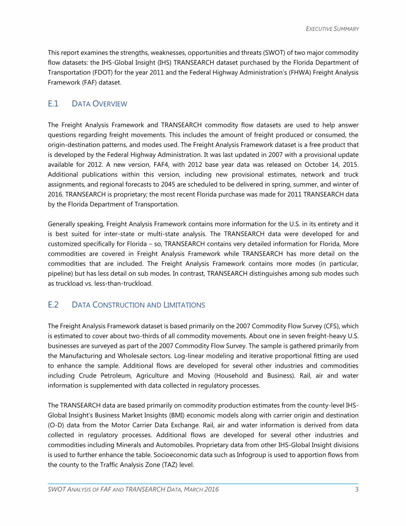
This report examines the strengths, weaknesses, opportunities and threats (SWOT) of two major commodity
flow datasets: the IHS-Global Insight (IHS) TRANSEARCH dataset purchased by the Florida Department of
Transportation (FDOT) for the year 2011 and the Federal Highway Administration’s (FHWA) Freight Analysis
Framework (FAF) dataset.
E.1 DATA OVERVIEW
The Freight Analysis Framework and TRANSEARCH commodity flow datasets are used to help answer
questions regarding freight movements. This includes the amount of freight produced or consumed, the
origin-destination patterns, and modes used. The Freight Analysis Framework dataset is a free product that
is developed by the Federal Highway Administration. It was last updated in 2007 with a provisional update
available for 2012. A new version, FAF4, with 2012 base year data was released on October 14, 2015.
Additional publications within this version, including new provisional estimates, network and truck
assignments, and regional forecasts to 2045 are scheduled to be delivered in spring, summer, and winter of
2016. TRANSEARCH is proprietary; the most recent Florida purchase was made for 2011 TRANSEARCH data
by the Florida Department of Transportation.
Generally speaking, Freight Analysis Framework contains more information for the U.S. in its entirety and it
is best suited for inter-state or multi-state analysis. The TRANSEARCH data were developed for and
customized specifically for Florida – so, TRANSEARCH contains very detailed information for Florida, More
commodities are covered in Freight Analysis Framework while TRANSEARCH has more detail on the
commodities that are included. The Freight Analysis Framework contains more modes (in particular,
pipeline) but has less detail on sub modes. In contrast, TRANSEARCH distinguishes among sub modes such
as truckload vs. less-than-truckload.
E.2 DATA CONSTRUCTION AND LIMITATIONS
The Freight Analysis Framework dataset is based primarily on the 2007 Commodity Flow Survey (CFS), which
is estimated to cover about two-thirds of all commodity movements. About one in seven freight-heavy U.S.
businesses are surveyed as part of the 2007 Commodity Flow Survey. The sample is gathered primarily from
the Manufacturing and Wholesale sectors. Log-linear modeling and iterative proportional fitting are used
to enhance the sample. Additional flows are developed for several other industries and commodities
including Crude Petroleum, Agriculture and Moving (Household and Business). Rail, air and water
information is supplemented with data collected in regulatory processes.
The TRANSEARCH data are based primarily on commodity production estimates from the county-level IHS-
Global Insight’s Business Market Insights (BMI) economic models along with carrier origin and destination
(O-D) data from the Motor Carrier Data Exchange. Rail, air and water information is derived from data
collected in regulatory processes. Additional flows are developed for several other industries and
commodities including Minerals and Automobiles. Proprietary data from other IHS-Global Insight divisions
is used to further enhance the table. Socioeconomic data such as Infogroup is used to apportion flows from
the county to the Traffic Analysis Zone (TAZ) level.
EXECUTIVE SUMMARY
SWOT ANALYSIS OF FAF AND TRANSEARCH DATA, MARCH 2016 4
Both datasets have the following limitations:
» They rely on data samples, which may lack information for certain industries, geographic areas, or
commodities;
» They use modeling processes in which uncertainty is inherent;
» Assumptions and judgment are intrinsic to the estimation process, introducing additional
uncertainty.
Because of these limitations, the data should not be treated as factual information but as estimates. It is
good practice to present and describe analysis results as estimates. It is also good practice to check the flow
estimates against other sources such as truck counts at Weight In Motion (WIM) stations.
E.3 USER GUIDANCE
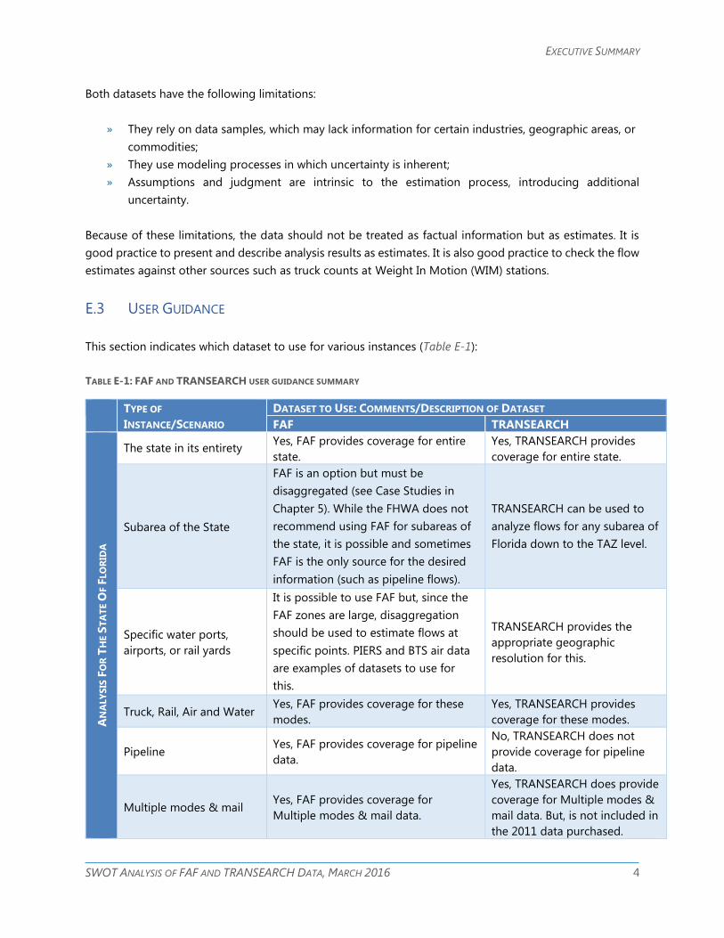
This section indicates which dataset to use for various instances (Table E-1):
TABLE E-1: FAF AND TRANSEARCH USER GUIDANCE SUMMARY
TYPE OF
INSTANCE/SCENARIO
DATASET TO USE: COMMENTS/DESCRIPTION OF DATASET
FAF TRANSEARCH
AN
ALY
SIS
FO
R T
HE S
TA
TE O
F F
LO
RID
A
The state in its entirety Yes, FAF provides coverage for entire
state.
Yes, TRANSEARCH provides
coverage for entire state.
Subarea of the State
FAF is an option but must be
disaggregated (see Case Studies in
Chapter 5). While the FHWA does not
recommend using FAF for subareas of
the state, it is possible and sometimes
FAF is the only source for the desired
information (such as pipeline flows).
TRANSEARCH can be used to
analyze flows for any subarea of
Florida down to the TAZ level.
Specific water ports,
airports, or rail yards
It is possible to use FAF but, since the
FAF zones are large, disaggregation
should be used to estimate flows at
specific points. PIERS and BTS air data
are examples of datasets to use for
this.
TRANSEARCH provides the
appropriate geographic
resolution for this.
Truck, Rail, Air and Water Yes, FAF provides coverage for these
modes.
Yes, TRANSEARCH provides
coverage for these modes.
Pipeline Yes, FAF provides coverage for pipeline
data.
No, TRANSEARCH does not
provide coverage for pipeline
data.
Multiple modes & mail Yes, FAF provides coverage for
Multiple modes & mail data.
Yes, TRANSEARCH does provide
coverage for Multiple modes &
mail data. But, is not included in
the 2011 data purchased.
EXECUTIVE SUMMARY
SWOT ANALYSIS OF FAF AND TRANSEARCH DATA, MARCH 2016 5
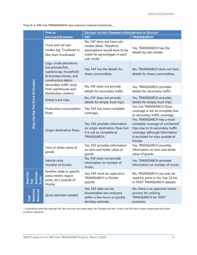
TABLE E-1: FAF AND TRANSEARCH USER GUIDANCE SUMMARY CONTINUED…
TYPE OF
INSTANCE/SCENARIO
DATASET TO USE: COMMENTS/DESCRIPTION OF DATASET
FAF TRANSEARCH A
NA
LY
SIS
FO
R T
HE S
TA
TE O
F F
LO
RID
A
Truck and rail sub-
modes (eg. Truckload vs.
less-than-truckloads)
No, FAF does not have sub-
modes detail. Therefore,
assumptions would have to be
made for percentages in each
sub-mode.**
Yes, TRANSEARCH has the
details by sub-modes.
Logs, crude petroleum,
live animals/fish,
waste/scrap, household
& business moves, and
construction debris
Yes, FAF has the details for
these commodities.
No, TRANSEARCH does not have
details for these commodities.
Secondary traffic (trips
from warehouses and
distribution centers)
No, FAF does not provide
details for secondary traffic.
Yes, TRANSEARCH provides
details for secondary traffic.
Empty truck trips No, FAF does not provide
details for empty truck trips.
Yes, TRANSEARCH provides
details for empty truck trips.
Production-consumption
flows
Yes, FAF has more complete
coverage.
Yes, but TRANSEARCH flows
coverage is not as complete due
to secondary traffic coverage.
Origin-destination flows
Yes, FAF provides information
on origin-destination flows but
it is not as complete as
TRANSEARCH.
Yes, TRANSEARCH has a more
complete coverage of unchained
trips due to its secondary traffic
coverage, although information
is excluded for trips outside of
Florida
Tons or dollar value of
goods
Yes, FAF provides information
on tons and dollar value of
goods.
Yes, TRANSEARCH provides
information on tons and dollar
value of goods.
Vehicle units
(number of trucks)
No, FAF does not provide
information on number of
trucks.
Yes, TRANSEARCH provides
information on number of trucks.
AN
ALY
SIS
FO
R
AN
OT
HER
ST
AT
E
Another state or specific
areas (metro region,
ports, etc.) outside of
Florida
Yes, FAF must be used since
TRANSEARCH is Florida-
specific
No, TRANSEARCH can only be
used for ports in the Top-10 list
in FDOT TRANSEARCH dataset.
TIM
E
SEN
SIT
IVE
AN
ALY
SIS
Quick estimate needed
Yes, FAF data can be
downloaded and analyzed
within a few hours to quickly
develop estimate.
No, there is an approval review
process for utilizing
TRANSEARCH for FDOT
purposes.
** It should be noted that although FAF does not have sub-modes detail, the “Multiple and Mail” mode in the FAF data include containerized and trailer-
on-flatcar shipments.

EXECUTIVE SUMMARY
SWOT ANALYSIS OF FAF AND TRANSEARCH DATA, MARCH 2016 6
INTENTIONALLY LEFT BLANK

SWOT ANALYSIS OF FAF AND TRANSEARCH DATA, MARCH 2016 7
CHAPTER 1
INTRODUCTION

INTRODUCTION
SWOT ANALYSIS OF FAF AND TRANSEARCH DATA, MARCH 2016 8
INTENTIONALLY LEFT BLANK
INTRODUCTION
SWOT ANALYSIS OF FAF AND TRANSEARCH DATA, MARCH 2016 9
This report provides a SWOT analysis of two major commodity flow datasets: the IHS TRANSEARCH dataset
purchased by FDOT for the year of 2011 for the state of Florida and the FAF dataset developed by FHWA.
Understanding the strengths and weaknesses of these datasets in comparison to each other is critical since
these are the most widely used commodity flow datasets in transportation planning. In order to make
informed decisions on data purchases and data use policies, FDOT needs to understand how each dataset
can support planning, policy and data analysis for freight, trade, and mobility.
As part of this effort, the RS&H Team provided an update to FSUTMS Model Task Force attendees at its
May 5-7, 2015 meeting in Orlando. RS&H presented the work to both the Freight Subcommittee on May
5th and the general audience on May 6th.
1.1 DEFINITIONS OF SWOT COMPONENTS
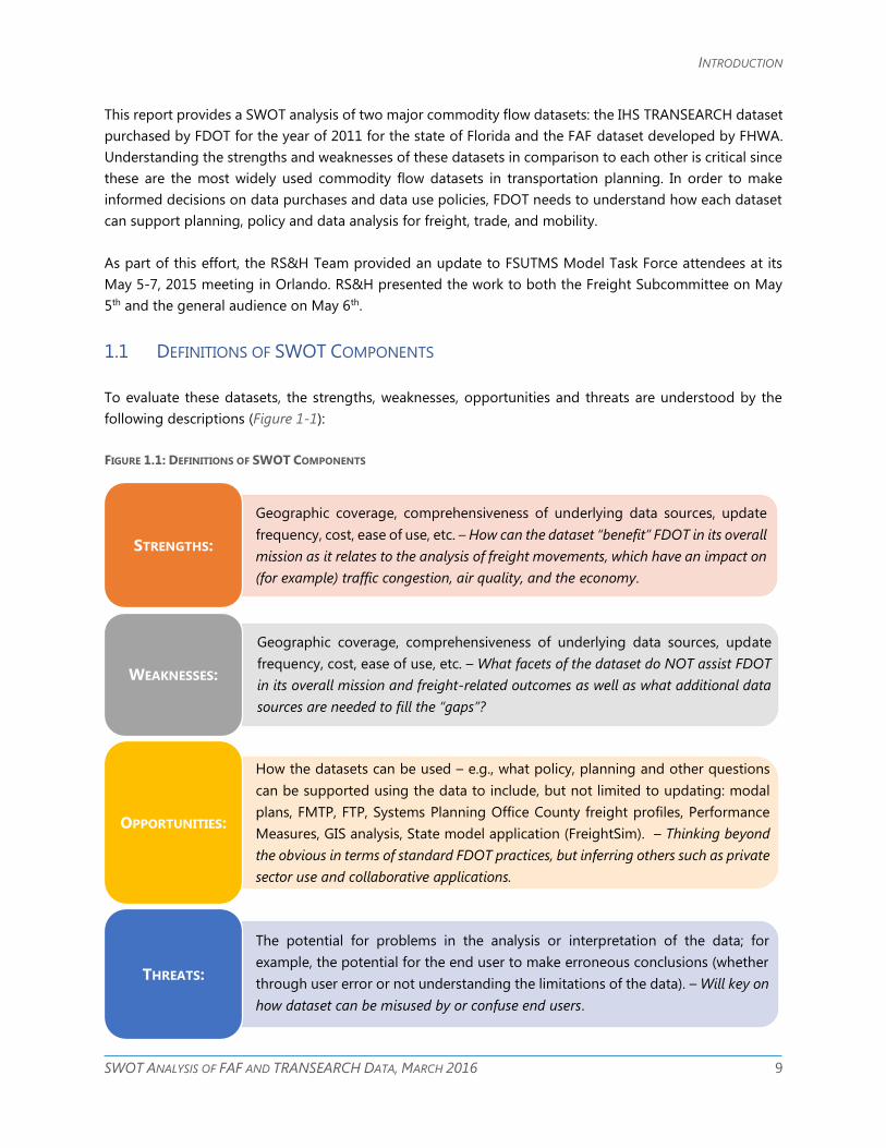
To evaluate these datasets, the strengths, weaknesses, opportunities and threats are understood by the
following descriptions (Figure 1-1):
FIGURE 1.1: DEFINITIONS OF SWOT COMPONENTS
STRENGTHS:
WEAKNESSES:
OPPORTUNITIES:
THREATS:
Geographic coverage, comprehensiveness of underlying data sources, update
frequency, cost, ease of use, etc. – How can the dataset “benefit” FDOT in its overall
mission as it relates to the analysis of freight movements, which have an impact on
(for example) traffic congestion, air quality, and the economy.
Geographic coverage, comprehensiveness of underlying data sources, update
frequency, cost, ease of use, etc. – What facets of the dataset do NOT assist FDOT
in its overall mission and freight-related outcomes as well as what additional data
sources are needed to fill the “gaps”?
How the datasets can be used – e.g., what policy, planning and other questions
can be supported using the data to include, but not limited to updating: modal
plans, FMTP, FTP, Systems Planning Office County freight profiles, Performance
Measures, GIS analysis, State model application (FreightSim). – Thinking beyond
the obvious in terms of standard FDOT practices, but inferring others such as private
sector use and collaborative applications.
The potential for problems in the analysis or interpretation of the data; for
example, the potential for the end user to make erroneous conclusions (whether
through user error or not understanding the limitations of the data). – Will key on
how dataset can be misused by or confuse end users.
INTRODUCTION
SWOT ANALYSIS OF FAF AND TRANSEARCH DATA, MARCH 2016 10
1.2 INTRODUCTION TO COMMODITY FLOW DATASETS
Commodity flow data refers to data that illustrate the amount of goods that flow between origins and
destinations. In this context, “goods” may be raw products such as corn, natural gas, sand, or phosphates;
intermediate goods such as textiles, steel, or lumber; or finished products including clothing, furniture or
newspapers.
The most commonly used commodity flow datasets in transportation planning are the IHS TRANSEARCH
database and the FHWA FAF database.
The FAF dataset contains flow estimates by mode of transportation for 43 commodity types, 131 origins
and 131 destinations. Annual dollars and tons are estimated and can be tabulated to, from, and within
regions. Provisional estimates are available for the current year with forecasts to 2040. The TRANSEARCH
database is similar in its overall structure but provides greater geographic and commodity detail per agency
needs.
The primary sources of commodity flow information are:
» Studies of companies that ship commodities;
» Surveys of carriers, or companies that transport shipments; and
» Information that is reported through regulatory processes, such as Customs data.
Each of these sources has major gaps. For example, in a survey, data is only collected from a sample of
companies. Further, regulatory processes typically cover shipments only for one mode or market (such as
import/export shipments that pass through a seaport). To overcome these gaps, the developers of FAF and
TRANSEARCH employ additional methods that help expand the data to cover the universe of commodity
flows. The principal methods used are:
» FAF: Iterative proportional fitting (IPF), log-linear modeling (LLM), gravity models and adjustments
based on the Bureau of Economic Analysis (BEA) Input/Output Make and Use tables; and
» TRANSEARCH: an economic model of commodity productions and consumptions by county (based
on IHS Economics’ BMI database), gravity models and adjustments based on the BEA Input/Output
Make and Use tables.
1.3 REPORT OUTLINE
This report is broken down into three more chapters as outlined below:
» Chapter 2 – Data Development explains the processes used to develop each dataset and details the
quality control checks of the datasets.
» Chapter 3 – SWOT Analysis compares the strengths and weaknesses of the datasets and summarizes
what each dataset offers.
» Chapter 4 – User Guidance provides training recommendations for a broad base of users.
SWOT ANALYSIS OF FAF AND TRANSEARCH DATA, MARCH 2016 11
CHAPTER 2
DATA DEVELOPMENT

DATA DEVELOPMENT
SWOT ANALYSIS OF FAF AND TRANSEARCH DATA, MARCH 2016 12
INTENTIONALLY LEFT BLANK

DATA DEVELOPMENT
SWOT ANALYSIS OF FAF AND TRANSEARCH DATA, MARCH 2016 13
2.1 INTRODUCTION
Commodity flows pertain to the movement of goods. Both the FAF3 and the TRANSEARCH datasets include
commodity shipments that are generated by companies that harvest, extract, or otherwise produce goods
that are then shipped to a point of use or consumption. While wholesale distributors and merchants do not
produce or consume goods, they receive and sell shipped goods. As such, they are an important sector in
goods movement. Table 2-1 lists various industry sectors using the North American Industry Classification
System (NAICS) and indicates whether each sector is a major generator of commodity shipments.
TABLE 2-1: INDUSTRY SECTORS IN THE 2012 NAICS CODING SYSTEM
2012
NAICS
CODE
2012 NAICS US TITLE
MAJOR
PRODUCER OF
COMMODITIES?*
11 Agriculture, Forestry, Fishing and Hunting Yes
21 Mining, Quarrying, and Oil and Gas Extraction Yes
22 Utilities No
23 Construction Moderate
31-33 Manufacturing Yes
42 Wholesale Trade Yes
44-45 Retail Trade Moderate
48-49 Transportation and Warehousing No
51 Information No
52 Finance and Insurance No
53 Real Estate and Rental and Leasing No
54 Professional, Scientific, and Technical Services No
55 Management of Companies and Enterprises No
56 Administrative and Support and Waste Management and Remediation
Services No
61 Educational Services No
62 Health Care and Social Assistance No
71 Arts, Entertainment, and Recreation No
72 Accommodation and Food Services No
81 Other Services (except Public Administration) No
92 Public Administration No * FAF and TRANSEARCH documentation were utilized to determine freight-heavy NAICS industries.
This chapter presents a summary of the methods used to construct each dataset. Information from existing
documentation is summarized. The existing reports describe how commodity shipments, including their O-
D patterns, are estimated for various industries. These shipments, which are generated by individual
establishments, are summarized at a zonal level to estimate the total O-D volumes for each commodity. In
addition, existing QA/QC checks of the data and existing comparisons of TRANSEARCH and FAF are
documented.
DATA DEVELOPMENT
SWOT ANALYSIS OF FAF AND TRANSEARCH DATA, MARCH 2016 14
The principal reports that are examined in this section are:
» Documentation of the FAF Database Construction: The Freight Analysis Framework Version 3 (FAF3):
A Description of the FAF3 Regional Database And How It Is Constructed. Prepared for the FHWA.
Prepared by Frank Southworth, Bruce E. Peterson, Ho-Ling Hwang, Shih-Miao Chin, & Diane
Davidson, Oak Ridge National Laboratory. June 16, 2011.
» Documentation of the TRANSEARCH Database Construction:
» TRANSEARCH 2011 Modeling Methodology Documentation. Prepared for FDOT. Prepared
by IHS, Inc. February 28, 2014.
» IHS TRANSEARCH TRAINING: Statewide TRANSEARCH & Freight Data Workshop. Delivered
by IHS, Inc. staff. May 14, 2014.
» The BCC Engineering TRANSEARCH Review: IHS Global TRANSEARCH: Data Review and
Analysis. Prepared for the Florida Department of Transportation Systems Planning Office.
Prepared by BCC Engineering, Inc. September 2014.
2.2 DATA DEVELOPMENT: 2007 FAF (FAF3)
The primary data source used to construct the 2007 FAF dataset is the 2007 U.S. Census CFS. In the CFS,
each business provides shipment information for one week in each quarter of the year. Roughly 12 million
domestic shipments across air, rail, highway and water modes are obtained in this survey. This information
is used to generate a snapshot of shipment activity in the U.S.
2.2.1 THE 2007 COMMODITY FLOW SURVEY (CFS)
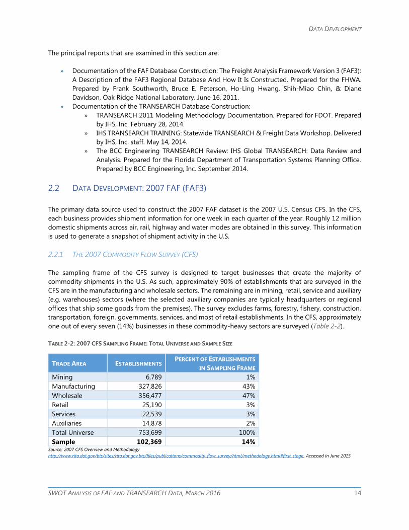
The sampling frame of the CFS survey is designed to target businesses that create the majority of
commodity shipments in the U.S. As such, approximately 90% of establishments that are surveyed in the
CFS are in the manufacturing and wholesale sectors. The remaining are in mining, retail, service and auxiliary
(e.g. warehouses) sectors (where the selected auxiliary companies are typically headquarters or regional
offices that ship some goods from the premises). The survey excludes farms, forestry, fishery, construction,
transportation, foreign, governments, services, and most of retail establishments. In the CFS, approximately
one out of every seven (14%) businesses in these commodity-heavy sectors are surveyed (Table 2-2).
TABLE 2-2: 2007 CFS SAMPLING FRAME: TOTAL UNIVERSE AND SAMPLE SIZE
TRADE AREA ESTABLISHMENTS PERCENT OF ESTABLISHMENTS
IN SAMPLING FRAME
Mining 6,789 1%
Manufacturing 327,826 43%
Wholesale 356,477 47%
Retail 25,190 3%
Services 22,539 3%
Auxiliaries 14,878 2%
Total Universe 753,699 100%
Sample 102,369 14% Source: 2007 CFS Overview and Methodology
http://www.rita.dot.gov/bts/sites/rita.dot.gov.bts/files/publications/commodity_flow_survey/html/methodology.html#first_stage, Accessed in June 2015
DATA DEVELOPMENT
SWOT ANALYSIS OF FAF AND TRANSEARCH DATA, MARCH 2016 15
For industrial sectors that produce two or more commodities, I/O make-and-use tables were used to
estimate the production volume of each commodity type. State and county data on production (sales,
employment, etc.) were used to help allocate flows between origins and destinations. Spatial allocation
formulas were then used to produce O-D flow volumes and distribute flows across counties for cross-FAF3
regional boundary issues.
However, the CFS has the following gaps, which are referred to as the Out-of-Scope (OOS) flows:
» Multi-Modal Truck, Rail & Water Flows associated with: Crude Petroleum, Petroleum Products &
Natural Gas Flows
» Truck-Only Flows associated With: Farm Based, Fisheries, Logging, Construction, Retail, Services,
Municipal Solid Waste, and Household & Business Moves
» International (Import & Export) Flows:
» Deep Sea Shipping Flows
» Air Freight Flows
» Transborder Truck & Rail Flows
It is estimated that OOS flows represent about 32% of all U.S. tons shipped. Due to the significance of this
figure, steps were taken to fill these data gaps in FAF. Data for OOS flows are mostly derived from data
reported by freight carriers. In some cases, secondary or indirect data (such as industrial activity,
employment or population) are used to allocate flows to specific geographic regions.
In addition, the CFS in-scope flow data have gaps where survey data are missing or where the sample size
is too small to report. Missing cells are filled using a combination of LLM and IPF.
2.2.2 ESTIMATION OF NON-CFS (OOS) DOMESTIC FLOWS
U.S. freight shipping establishments in the following industrial sectors were not surveyed as part of the 2007
US Commodity Flow Survey. The following OOS industries therefore had to be assigned commodity and
mode specific O-D flows using other methods:
» Farm Based
» Fishery
» Logging
» Construction
» Services
» Retail
» Household and Business Moves
» Municipal Solid Waste
» Crude Petroleum
» Natural Gas Products
Flows for these OOS industries were estimated in FAF3 using the following process:
» Step 1—Estimate national shipments totals for each industry by FAF3 commodity classes
» Step 2—Regionalize these national shipments (by ton and value) down to the level of U.S. counties
» Step 3—Estimate O-D flows at the county level
» Step 4—Aggregate the O-D estimates from counties back up to FAF3 region-to-region flows.

DATA DEVELOPMENT
SWOT ANALYSIS OF FAF AND TRANSEARCH DATA, MARCH 2016 16
The specific details in the above process vary by sector as follows.
2.2.2.1 Farms
Farm-based flows are assumed to be moved entirely by truck. They are assumed to be nearly all farm-to-
storage or farm-to-distribution/processing center. FAF3 tons and dollars shipped were estimated using
county and state data published in the U.S. Department of Agriculture’s (USDA) 2007 Census of Agriculture
and the 2008 Agricultural Statistics. The information was supplemented with data from USDA’s Statistical
Bulletins. Origin totals (produced at farms) are derived from USDA county production data with gaps filled
in using acreage by county devoted to specific crops. Destination totals (at storage and processing centers,
such as grain elevators) are derived from 2007 CFS agricultural commodity originations, which typically are
reported at storage/DC/processing centers. O-D flows are then estimated using 2002 Vehicle Inventory and
Use Survey (VIUS) truck trip length distributions.
2.2.2.2 Fisheries
Fishery flows are based on port data for commercial landings by US fisherman. The process relies mainly on
statistics published in the Fisheries of the United States 2008, an annual report prepared by the National
Marine Fisheries Service (NMFS) of the National Oceanic and Atmospheric Administration (NOAA).
Northwestern Pacific (near Washington, Oregon, and Alaska) fish that are processed on-board are credited
to landing in the state nearest the capture.
Fish movements are assumed to be all local & all truck.
2.2.2.3 Construction, Services, Retail, and Household and Business Moves
Flows associated with the Construction, Services, Retail, and Household and Business Moves sectors were
developed for FAF3 by MacroSys, LLC using 2002 US I-O Make and Use tables. Dollar values from Make and
Use tables were converted to tonnages using 2007 CFS for similar commodities and other industry-specific
data sources.
These flows were assumed to be all truck. Also, only domestic shipments were estimated.
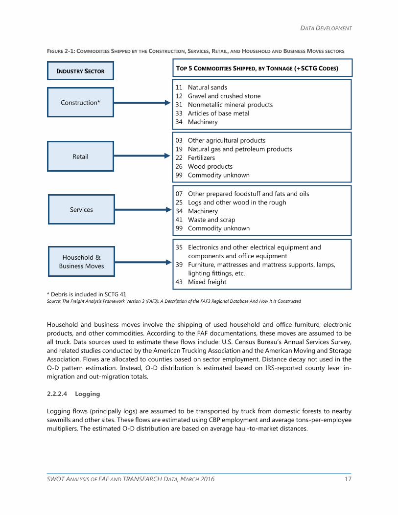
Figure 2-1 shows the top five commodities are assumed to be shipped by the Construction, Services, Retail,
and Household and Business Moves sectors.
For the construction industry, debris estimates are developed using U.S. Environmental Protection Agency
(EPA) publications, the National Demolition Association, Construction Materials Recycling Association, and
Gershman, Brickner & Bratton, Inc. Shipment volumes were assigned to FAF3 regions based on: sales data
from the 2007 Economic Census; 2007 county level employment data from the Census Bureau’s County
Business Patterns (CBP) dataset, multiplied by Census-developed labor productivity rates by industry class.
Volumes of these goods are assumed to begin and end within the same FAF zone.
It is estimated that the Service Sector generates significant amounts of both commodity freight and mail.
Non-mail attractions are based on industrial employment and the amount of commodities used by
industries according to the Use table. A gravity model is used to distribute flows of the non-mail
commodities. Mail attractions are based on total service employment; i.e., mail is assumed to be shipped
from one service establishment to another service establishment. There is no distance decay effect.
DATA DEVELOPMENT
SWOT ANALYSIS OF FAF AND TRANSEARCH DATA, MARCH 2016 17
FIGURE 2-1: COMMODITIES SHIPPED BY THE CONSTRUCTION, SERVICES, RETAIL, AND HOUSEHOLD AND BUSINESS MOVES SECTORS
* Debris is included in SCTG 41 Source: The Freight Analysis Framework Version 3 (FAF3): A Description of the FAF3 Regional Database And How It Is Constructed
Household and business moves involve the shipping of used household and office furniture, electronic
products, and other commodities. According to the FAF documentations, these moves are assumed to be
all truck. Data sources used to estimate these flows include: U.S. Census Bureau’s Annual Services Survey,
and related studies conducted by the American Trucking Association and the American Moving and Storage
Association. Flows are allocated to counties based on sector employment. Distance decay not used in the
O-D pattern estimation. Instead, O-D distribution is estimated based on IRS-reported county level in-
migration and out-migration totals.
2.2.2.4 Logging
Logging flows (principally logs) are assumed to be transported by truck from domestic forests to nearby
sawmills and other sites. These flows are estimated using CBP employment and average tons-per-employee
multipliers. The estimated O-D distribution are based on average haul-to-market distances.
Construction*
Retail
Services
Household &
Business Moves
11 Natural sands
12 Gravel and crushed stone
31 Nonmetallic mineral products
33 Articles of base metal
34 Machinery
03 Other agricultural products
19 Natural gas and petroleum products
22 Fertilizers
26 Wood products
99 Commodity unknown
07 Other prepared foodstuff and fats and oils
25 Logs and other wood in the rough
34 Machinery
41 Waste and scrap
99 Commodity unknown
35 Electronics and other electrical equipment and
components and office equipment
39 Furniture, mattresses and mattress supports, lamps,
lighting fittings, etc.
43 Mixed freight
INDUSTRY SECTOR TOP 5 COMMODITIES SHIPPED, BY TONNAGE (+SCTG CODES)
DATA DEVELOPMENT
SWOT ANALYSIS OF FAF AND TRANSEARCH DATA, MARCH 2016 18
2.2.2.5 Municipal Solid Waste
Examples of Municipal solid waste (MSW):
» Containers and packaging, such as soft drink bottles and cardboard boxes,
» Durable goods, such as furniture and appliances,
» Nondurable goods, such as newspapers, trash bags, and clothing, and
» Other wastes, such as food scraps and yard trimmings.
MSW shipments are based on information from Franklin Associates in collaboration with the U.S. EPA and
information in the BioCycle journal. Mode specific data was also obtained from the U.S Army Corps of
Engineers Waterborne Commerce statistics, and from the Surface Transportation Board’s Railcar Waybill
sample.
All MSW is collected at the source and transported to one of four types of processing facility: local landfills,
local incineration facilities, local material recovery facilities, and waste transfer stations. Garbage trucks are
assumed to unload MSW at these processing sites for accumulation and transfer to larger transport vehicles
(truck, rail, or barge), for more economical long-distance hauling to a final disposal site.
State-to-state O-D flows of MSW are estimated using Congressional Research Service information and
discussions with ORNL staff and local officials. These flows are mostly truck movements but a large amount
longer distance, inter-state shipments are by rail or barge; still, this is less than 4% of all MSW shipments.
O-D estimation for truck-only MSW between FAF3 regions below state level used county population and
spatial interaction models; average O-D distance assumed to be about 32 miles based on the documented
sources.
2.2.2.6 Crude Petroleum
Crude petroleum shipments originate at domestic oil fields or marine terminals where foreign oil imports
arrive. These shipments are delivered to either refineries or long-term storage facilities.
Prominent modes in shipping crude petroleum include: pipeline, marine vessels (inland barge and ocean
tankers), rail tanker, and tanker trucks. National data on shipments by mode from Shifts in Petroleum
Transportation, an annual report published by Association of Oil Pipelines. Information in the Shifts report
is based on:
» Oil Pipelines: Annual Report of oil pipeline companies provided to the Federal Energy Regulatory
Commission (FERC Form 6);
» Water Carriers: Waterborne Commerce of the United States, U.S. Army Corps of Engineers (USACE);
» Motor Carriers: Petroleum Tank Truck Carriers Annual Report, American Trucking Association, Inc.
and Petroleum Supply Annual, Energy Information Administration (EIA); and
» Railroads: Carload Waybill Statistics, Report TD-1, USDOT, Federal Railroad Administration, and
Freight Commodity Statistics, Association of American Railroads.

DATA DEVELOPMENT
SWOT ANALYSIS OF FAF AND TRANSEARCH DATA, MARCH 2016 19
O-D flows are derived from US DOE/EIA information, including EIA's Petroleum Supply Annual (2010) data
on:
» Production of Crude oil by PADD (Petroleum Administration for Defense Districts) and State,
» Refinery Input of Crude Oil by Refining Districts, and
» Refinery Receipts of Crude Oil by Method of Transportation, by PADD.
In the flow estimation process, first domestic crude production and inputs are estimated at FAF3 regional
level. Second, a gravity model is used to estimate O-D between FAF3 regions. Third, flows are apportioned
by mode using "interactive proportional process". Domestic mode shares were informed using EIA’s
Refinery Receipts table (which has mode shares by district) and EIA's Movements of Crude Oil between
PADD.
2.2.2.7 Natural Gas Products
Total National Natural Gas and O-D region-to-region flows are derived from EIA's 2010 Natural Gas Annual,
which includes gas productions or "gross withdrawals" by state and Gulf of Mexico. The estimation of O-D
distribution patterns is similar to the estimation process for crude petroleum.
2.2.3 IMPORTS AND EXPORTS
Imports are commodities that are transported from another country into the United States and exports are
commodities that are transported from the United States to a foreign country.
Import and export flows are generally constructed for FAF using mode-specific data sources: airborne,
waterborne, and land-based (border-crossing, mainly truck and rail) datasets. Import and export flow
estimates of crude petroleum and natural gas are developed separately.
2.2.3.1 Water
Water imports and exports are developed for FAF using:
» The USACE International Waterborne Commerce Database
» The US Census Bureau’s Foreign Trade Database
» A FAF3-specific extraction of state-to/from-US port data from the Port Import Export Reporting
Service (PIERS) Import/Export Database; at its base, PIERS data is from shipment records collected
by US Customs and Border Protection
Since the PIERS dataset contains the most O-D and commodity specificity, the PIERS data (after some
adjustments to the raw data) are the basis of the FAF waterborne flows. PIERS tonnages were adjusted to
be consistent with USACE waterborne tonnages and PIERS dollar trades to be consistent with Census FTD
totals. Geocoding was adjusted to infer (1) zip codes when this information was missing; and (2) the correct
origination/termination when company headquarters was reported in the documentation. These inferences
were made based on patterns from the 2007 CFS. The developers of FAF consider these geocoding issues
to be a major concern with additional research needed to understand the extent of the misreporting.
Inland mode is generally not available for the PIERS information. The exception occurs for PIERS shipments
that reported usage of rail-inclusive container shipments were treated as truck-rail IMX (i.e., "multiple
DATA DEVELOPMENT
SWOT ANALYSIS OF FAF AND TRANSEARCH DATA, MARCH 2016 20
mode") in FAF3. It is not clear from the FAF documentation how inland mode is inferred for other shipment
records.
2.2.3.2 Air
Airport-to-airport flows of air-based imports and exports are determined using total tonnage statistics from
the T-100 dataset published by the Office of Airline Information (OAI) of the U.S. Bureau of Transportation
Statistics (BTS) along with US Customs data on commodities and value of goods shipped as reported by
Foreign Trade Division (FTD) of the U.S. Department of Commerce’s Bureau of the Census.
The FTD database includes shipments for all merchandise between foreign countries and US Customs
Territories (typically at state level & Washington, DC). Available information includes the value, quantity,
method of transportation, and shipping weights for some 9,000 export commodities, 17,000 imported
commodities, 240 trading partners, and 45 U.S. Customs Districts. The two FTD databases used are the U.S.
Exports of Merchandise – Monthly and U.S. Imports of Merchandise – Monthly.
The Bureau of Transportation Statistics OAI T-100 Data is the definitive source of tonnages shipped on US
airlines. The dataset includes ports of entry/exit but lacks ultimate origin/destination of shipments with
multiple stops. Since it also lacks information on value and commodity type, this information was obtained
from US Customs FTD data then combined with the OAI data.
Spatial and commodity information in the OAI and FTD data were reconciled to create a single FAF3 air O-
D flow dataset. Control totals for the flows were based on OAI total tonnages and FTD commodity
percentages. FTD data were also used to assign and value-to-weight ratios.
Some quality issues with the OAI and FTD data were noted. First, while the FTD dataset does not include
transshipments the OAI data does. Large differences between the datasets are observed at major
transshipment airports (Anchorage, Miami, New York). Other issues are:
» OAI is missing information for some all-cargo airlines;
» FAF may double-count some mail shipments (as both mail and freight) since FedEx includes mail as
part of total freight when reporting to OAI;
» Since OAI is carrier-based, shipments using two or more carriers will have incorrect origin and/or
destination information; and
» While in-transit shipments are supposed to be completely excluded from the data, intermediate
stops of in-transit shipments may sometimes be reported as the origin or destination airport.
2.2.3.3 Truck and Rail
Overland movements (by truck & rail) between US and Canada/Mexico are from the BTS TransBorder Freight
Database, which is based on FTD trade data. The following tables are used:
» U.S. Trade with Canada and Mexico with State and Port Detail
» U.S. Trade with Canada and Mexico with State and Commodity Detail
» U.S. Trade with Canada and Mexico with Port and Commodity Detail
Modal detail is provided. To estimate truck and rail O-D flows, movements by vessel, air and pipeline were
first removed. Next, CBP information was used to allocate flows from states to FAF3 regions. When an FTD
DATA DEVELOPMENT
SWOT ANALYSIS OF FAF AND TRANSEARCH DATA, MARCH 2016 21
Port was not specified but the FTD Port District was known, flows were assigned to the most likely port for
that District on the basis of tons or dollars of a specific commodity passing through each port.
Shipment weights are not reported. Weights are estimated for FAF based on average dollar per ton statistics
by commodity class, mode and country.
2.2.3.4 Crude Petroleum
Imports of crude petroleum are reported to the EIA monthly at the company level. This information tracks
the complete movement of imported crude oil including the foreign source country, the U.S. port used, and
the refinery that is the domestic destination of the shipment. The company-level monthly EIA reporting is
used to establish O-D flow patterns.
U.S. flows are allocated to modes based on modal information from EIA refinery receipts. A single mode
was determined for each port-to-refinery pair. Flows between the foreign country and the U.S. port are
generally assumed to be made by ocean tankers. The exception is for Canada-to-U.S. flows, which are
assumed to be pipeline flows from Alberta and offshore of the Atlantic Ocean.
Data sources include:
» Form EIA-810: Monthly Refinery Report;
» Form EIA-814: Monthly Imports Report;
» Form EIA-815: Monthly Terminal Blenders Report;
» Form EIA-820: Annual Refinery Report; and
» The EIA State Level Production dataset.
2.2.3.5 Natural Gas
Liquefied Natural Gas (LNG) imports and exports are made using large tanker ships. EIA reports contain
information on directional LNG volumes by U.S. seaport, natural gas (NG) pipeline volumes between the
U.S. and Canada and Mexico, and total import/export volumes by state.
O-D patterns are determined using the EIA information along with CBP data. The FAF documentation notes
that there are very few inter-regional movements of imported or exported NG/LNG.
2.3 DATA DEVELOPMENT: 2011 TRANSEARCH
Like the FAF data, the TRANSEARCH dataset is developed with the goal of capturing commodity shipments
generated by various industry sectors. However, while the FAF development relies primarily a survey of
major freight-related industries, the TRANSEARCH development relies fundamentally on economic models
that are used to estimate the amount of each commodity that is produced and consumed in each U.S.
county. Volumes for non-truck modes, which constitute less than 50% of tonnages in Florida, are first
estimated based primarily on data from regulatory agencies. These non-truck volumes are then subtracted
from the total volume estimate to estimate truck volumes, which make up the majority of flows. As such,
the majority of commodity flows in TRANSEARCH are based primarily on the economic models with
enhancements from other sources.
Empty truck flows as well as truck flows for secondary shipments, agricultural products, coal, and chemicals
are derived from other sources. These are described in the Specialized Truck Flows section.
DATA DEVELOPMENT
SWOT ANALYSIS OF FAF AND TRANSEARCH DATA, MARCH 2016 22
Data from truck carriers, public sources, and other propriety sources are used to estimate O-D flow patterns.
2.3.1 COUNTY-LEVEL PRODUCTION AND CONSUMPTION VOLUMES
The IHS Economics’ BMI database is used to estimate output volumes by industry and commodity at the
county level. This database is supplemented with trade association and industry reports and U.S.
government-collected data. The estimated outputs are combined with information from the I/O tables to
estimate the values of goods produced and consumed in each county for each commodity.
The BMI-based methodology does not include all industries. Production volumes for the following
commodities are estimated using other sources:
» Agricultural products and livestock (sourced from the U.S. Department of Agriculture)
» Coal and automobiles (sourced from other IHS in-house databases)
» Selected chemicals (sourced from IHS Chemical group)
» Minerals (sourced from the U.S. Geological Survey).
In addition, import and export volumes are estimated using port-level census statistics. These volumes are
added into the domestic county-level estimates. Finally, demand levels from households, the public sector
and the financial sector are estimated based on tax revenue and similar sources then are also incorporated
into the county-level estimates.
2.3.2 COMMODITY FLOWS FOR RAIL, WATER AND AIR MODES
Commodity volumes for rail, water, air and pipeline moves are relatively well understood due to government
regulated reporting requirements. The O-D volumes by commodity for each mode are evaluated. Then,
these volumes are subtracted from the total volumes that were initially estimated. The remaining flows are
assumed to be transported using trucks and are allocated to truck O-D and distribution patterns. The non-
truck commodity flows are developed using the following processes.
2.3.2.1 Rail
Rail flows are developed using a survey of rail carload and intermodal shipments that were reported in the
Surface Transportation Board (STB) Waybill sample. There are two versions of the Waybill data. One is very
detailed and the other is less detailed. Two versions of TRANSEARCH were developed for FDOT, one with
each version of the Waybill data. Usage of the more detailed version requires special clearance from the
STB. While the Waybill data has full coverage of US-Canada rail flows, US-Mexico rail flows were derived
from BTS border crossing statistics as well as (indirectly) from Waybill routing information.
2.3.2.2 Water
Water shipments are estimated primarily using the U.S. Army Corps of Engineers annual waterborne
commerce data.
DATA DEVELOPMENT
SWOT ANALYSIS OF FAF AND TRANSEARCH DATA, MARCH 2016 23
2.3.2.3 Air
The BTS T-100 data set on airport activity is the primary information source for TRANSEARCH air-based
moves. The T-100 dataset provides total tonnages. Commodity details are derived from CFS information.
According to the TRANSEARCH documentation, the tonnages include only cargo that is drayed to or from
the airport.
2.3.3 TRUCK FLOWS
As described in the introduction, most truck-based commodity production and consumption volumes are
derived by subtracting rail, water and air moves from the total estimates of production and consumption
volumes. (Other truck-based commodity flows are described as Specialized Truck Flows and are discussed
in the next section.)
The truck-based productions and consumptions are distributed using a gravity model to create O-D flows.
The model inputs are (1) the production and consumption volumes and (2) trip length distributions for each
commodity from publicly available sources.
The estimated O-D flows from the gravity model are then validated using observed commodity flow
information collected by the carrier industry. The data source used is the Motor Carrier Data Exchange
program, which includes annual tonnage or truckloads for each O-D pair with information provided at the
zip code level. The Motor Carrier Data Exchange program data are further supplemented as follows. First,
for truck trip origins, the dataset is supplemented with proprietary data on industrial output, employment
and sales level data from specific locations of manufacturing and distribution facilities. Second, for truck
trip destinations / consumption locations, the dataset is supplemented with BEA Industrial I/O tables.
CFS information is used to allocate the percentage split between for-hire and private fleets. Data from the
Motor Carrier Data Exchange program are then used to infer the split of for-hire trips between truckload
and LTL and commodity type (where equipment – truck body type – is reported).
Since the Motor Carrier Data Exchange program dataset is critical to establishing truck flows, it is important
to understand it. The TRANSEARCH documentation reports that: "Participating carriers are primarily large
truckload and LTL operators with average lengths of haul over 500 miles. However, the sample also includes
owner-operator business, portions of private carriage and dray activity, and significant amounts of regional
(under 500-mile) traffic. The sampling rate is about 7% overall, 3% under 500 miles, and 1% under 100 miles.
(As another point of comparison, the STB Waybill Sample runs 2.8% of shipments, but it is a stratified
random sample and thus includes 22.5% of tonnage.)"
The TRANSEARCH documentation further notes that one drawback of the Motor Carrier Data Exchange
data is that the collected data does not constitute a stratified random sample. In other words, the data
might have insufficient coverage of certain markets. However, the documentation suggests that the
program’s diverse coverage across industrial and geographic segments helps compensate for this.
2.3.4 SPECIALIZED TRUCK FLOWS
Secondary Shipments, Agricultural Products, Coal, Chemicals, Automobiles, Minerals and Empty Movements
are considered Specialized Truck Flows. Unlike the other TRANSEARCH truck flows, these do not use the
BMI economic model. These flows are developing using alternative processes as described below.

DATA DEVELOPMENT
SWOT ANALYSIS OF FAF AND TRANSEARCH DATA, MARCH 2016 24
2.3.4.1 Secondary Shipments
Secondary shipments originate at intermediate handling locations such as warehouses, distribution centers,
or other non-production facilities. The ultimate destination of these shipments (where the commodity is
consumed or used) is mirrored in the TRANSEARCH data – for example, destinations in the dataset may be
manufacturing plants for raw materials, or supermarkets or department stores for consumer goods. In
reality, the shipment may move through a series of regional distribution centers or warehouses. However,
the source data do not permit the accurate identification of individual legs of this type of journey.
2.3.4.2 Agriculture
The main data sources used to develop agricultural production volumes are statistics on county production
by type of crop, product or livestock from the USDA. States with major agricultural industries provide
additional data. The documentation indicates that IHS Agriculture Crop Production and Forecasts is another
source of information. County-level consumption volumes are based on industry factors for agricultural
facilities such as grain elevators, processing businesses, and rail and water transfer points. County-level
consumption also reflects output portrayed elsewhere in TRANSEARCH. Agricultural flows are distributed
to O-D pairs based on historical patterns, which incorporate information on travel distances by use, product,
and body type.
2.3.4.3 Coal
Truck movements of coal are developed using information from the U.S. Department of Energy’s EIA. The
EIA datasets include state-to-state truck volumes and production and consumption information for
specific locations. Consumption is allocated more specifically based on relative consumption by industry
(manufacturing, power generation etc.). The TRANSEARCH documentation indicates that the proprietary
source Cambridge Energy Research Associates (CERA) Electric Plant Statistics and Forecasts provides
information on its energy analysis.
2.3.4.4 Chemicals
Truck movements of chemicals are developed using data from the IHS Chemical Group on production
volumes and plant information (the IHS Chemical Plant Production and Consumption Statistics). Intra-plant
and intra-company movements are accounted for.
2.3.4.5 Automobiles
Automobile flows by truck are developed using proprietary data from in-house IHS databases such as the
IHS Automotive Plant Production, Consumption, and Supplier Data.
2.3.4.6 Minerals
Truck transportation estimates of mineral flows are developed in part using U.S. Geological Survey Mineral
Industry Reports.

DATA DEVELOPMENT
SWOT ANALYSIS OF FAF AND TRANSEARCH DATA, MARCH 2016 25
2.3.4.7 Empty Trucks (Empties)
Empty truck movements are estimated for TRANSEARCH as follows. County imbalances of inbound and
outbound loads by trailer category are examined at the aggregate (nationwide) level. Results are checked
against market conditions and industry factors. Flows between the US and Canada/Mexico are developed
separately then combined with the U.S. dataset.
2.3.5 IMPORTS AND EXPORTS
Important data sources for determining import and export flows include:
» The BTS TransBorder Freight Database, which is constructed using FTD trade data;
» US Customs data on commodities and value of goods shipped (reported by Foreign Trade Division
(FTD) of the U.S. Department of Commerce’s Bureau of the Census);
» Data from the Mexico Economic Census (conducted by the Instituto Nacional de Estadística y
Geografía, or INEGI);
» The TRANSEARCH Data Exchange program
Overland U.S.-Mexico flows are enhanced using data from the Mexico Economic Census, internal IHS
Mexican intelligence, and cross border information from the TRANSEARCH Data Exchange program. Flows
are converted into truck and rail unit counts using averages from the data exchange or commodity specific
defaults. Flows are further adjusted where the data exchange contains additional information of observed
flows.
Water-based flows between the U.S. and Mexico are determined using BTS TransBorder data and statistics
for Mexican ports from the Mexican Secretaría de Comunicaciones y Transportes (SCT). While the overall
quality of the data and process are unclear, the results are then checked using US-Mexico truck traffic
Data from the TRANSEARCH Data Exchange information.
Flows between the U.S. and Canada rely primarily on the BTS TransBorder data, which reports truck, rail,
water, air, and pipeline, and "other" (unspecified) modes. (The U.S.-Mexico BTS data has truck, rail and
pipeline only.) These cross-border markets are the only areas of TRANSEARCH where pipeline data is
available; crude petroleum and natural gas are dominant in these moves.
For both Canadian and Mexican commodity moves, traffic volumes are used to allocate the flows to the
county level within the U.S. On the Canadian side, flows are allocated to metro areas based on Statistics
Canada truck traffic reports. Canadian O-D flows are apportioned to specific metropolitan markets based
on Canadian truck traffic data from Statistics Canada.
2.3.6 OTHER FLOWS – NOT COVERED
The standard TRANSEARCH product does not include the following shipments:
» Primary (raw) products of forests and fisheries;
» Household goods; and
» Haulage of waste and scrap.
DATA DEVELOPMENT
SWOT ANALYSIS OF FAF AND TRANSEARCH DATA, MARCH 2016 26
It is worth noting that commodities in these three categories are included in FAF, which is the source of
some tonnage differences between the two data sources.
2.3.7 APPORTIONMENT TO THE TAZ LEVEL
The TRANSEARCH commodity flow data are developed at the county level as described above. For the FDOT
2011 dataset purchase, the data were apportioned from the 67 Florida counties to Florida’s 8,518 TAZs.
Outbound flows are disaggregated from the county to TAZ level based on relative output (such as
employment or sales volumes) of commodity-generating industries in each TAZ. Inbound flows are
apportioned in a similar manner except that commodity-consuming industries are used instead of
commodity-producing industries.
The apportionment primarily utilized socio-economic data as well as establishment and industry data from
InfoUSA business listings. These data were supplemented with information from the IHS-Global Insight
Freight Finder tool, which contains tonnages for specific facilities.
Numerous assumptions were used in this process. The assumptions are described in detail in the
TRANSEARCH 2011 Modeling Methodology documentation on pages 19-22. For purposes of interpreting
the data for the SWOT analysis, key assumptions are:
» Secondary traffic:
» Distribution centers are often associated with low sales volumes. Presumably this happens
mostly at facilities that handle internal distribution where the passage of goods does not
involve sales activity.
If retailers belonging to the same company could be identified and if the retailer
sales volumes exceeded the distribution center sales volume, then the distribution
center sales volume was set to the total sales volume of the associated retailers.
For distribution centers with matched retailers, total inbound tons of secondary
traffic are set to match outbound tons of secondary traffic
If a distribution center could not be matched to a retailer, then total outbound tons
is set to match non-secondary inbound tons.
» Retailers are assumed to receive 80% of inbound goods from distribution centers (STCC
5010) and 20% from factories. Auto retailers are handled in a separate process.
» Volumes of less than 100 tons per year of a single commodity are considered Secondary
Traffic.
» Private truck assumptions: Inbound shipments to companies with large private fleets (not including
distribution centers) are assumed to be made by private truck. These companies are identified using
secondary data sources. The total TRANSEARCH private truck tonnage is maintained for each
county.
» Empty truck assumptions: Empty truck origins are assumed to be generated in the same proportion
as inbound loaded moves. Empty truck destinations are apportioned in a similar fashion using
outbound loaded moves. Equipment type and mode are considered.
» Industry assumptions:
» Retail facilities generally are assumed to have no outbound shipments. There are two
exceptions for this: brewpubs are assumed to ship beer and new car dealers ship small
volumes of cars to other dealers.
» Construction firms are assumed to receive no inbound goods at their offices, except for 2%
of sales of STCC 5010 for general office use.
DATA DEVELOPMENT
SWOT ANALYSIS OF FAF AND TRANSEARCH DATA, MARCH 2016 27
» Geocoding: Flows to headquarters, administrative facilities, PO boxes, and establishments on the
2nd story or higher are generally assumed to be non-existent.
» Modal assumptions:
» Proximity to a rail line is used to assign rail traffic.
» For each county, estimates of outbound rail tons of commodities in the 2011-3999 range
are adjusted to match total estimates of TRANSEARCH trucks.
» Air shipments are assigned to the TAZ for airports. The drayage of these shipments is then
assigned to warehouses in TAZs based on transportation and warehouse employment.
» By default, rail shipments are assigned to the TAZ in which the reported FRA 100k Network
node is located. This information is overridden for some major establishments including
power plants, copper mines and smelters, and auto ramps.
» Truck traffic to and from ports is assumed to begin and end in the TAZ in which the port is
located. TAZ allocation for ports that span multiple TAZs are further informed based on
ship location data (AIS) and PIERS data on port call information.
» Intermodal shipments are assigned to specific ramps in proportion to tons terminating at
each ramp. Customer establishments are assigned in proportion to truck flows by
commodity type as determined in the commodity flow development process.
» New motor vehicles are assigned to the TAZ of auto ramps to the extent they don’t exceed total
rail terminations. Mode is truckload or private.
Other assumptions, including assumptions made specifically for origin and destination TAZs, are further
detailed in the official documentation.
2.4 FORECASTING PROCEDURES
Both the FAF and TRANSEARCH data products include forecast commodity flows for a long-term horizon.
Projections for each dataset are largely consistent with the base year development with forecast totals
controlled by both U.S. and international trade patterns.
2.4.1 FAF FORECASTS
The FAF3 data suite includes baseline flow estimates for year 2007 and forecasts for 2015, 2020, 2025, 2030,
2035, and 2040.
The FAF forecasts are an extrapolation of baseline commodity flow trends with current flows projected to
the future based on national and global economic patterns.
The following processes are used to develop the forecasts:
» Using economic models, forecast national consumption and foreign trade patterns are converted
into purchase volumes across industries.
» Future mode shares are estimated by applying current mode shares by commodity to the
forecasted mix of commodities.

DATA DEVELOPMENT
SWOT ANALYSIS OF FAF AND TRANSEARCH DATA, MARCH 2016 28
The disadvantages of the methodology are that the forecasts do not reflect:
» Major changes in the national economy;
» Future limitations in capacity; or
» Changes in transportation costs, technology, or other aspects of the transportation system.
2.4.2 TRANSEARCH FORECASTS
The TRANSEARCH forecasts are developed for up to a 30-year time horizon. Forecast years include: 2015,
2020, 2025, 2030, 2035 and 2040. The methodology utilizes the forecasting tools of IHS Economics.
The TRANSEARCH forecasts are constructed using methods that are consistent with the base year
development – for example, through the use of BMI economic models. Like the FAF forecasts, the process
is consistent with forecasted national and global economic patterns.
The following processes are used to develop the forecasts (Figure 2-2):
Supply (freight originations) and demand (freight destinations) projections are estimated for each
county and commodity type using BMI forecasts. Employment, output, and purchases by industry
and county are included in the supply and demand estimates.
The aggregated county-level flows are constrained to national totals from the proprietary IHS U.S.
Macroeconomic long-term forecasts.
International flows are forecast using information from the World Trade Service, which includes
imports and exports to/from Canada and Mexico and at U.S. seaports.
The process is also informed by propriety data and services from IHS-Global Insight: U.S.
Agricultural Service, Energy Service, Automotive Service, World Trade Service, and the Business
Transactions Matrix (which contains forecasts of the BEA's I/O tables).
FIGURE 2-2: TRANSEARCH FORECAST DEVELOPMENT
Source: TRANSEARCH 2011 Modeling Methodology Documentation. Prepared for Florida DOT. Prepared by IHS, Inc. February 28, 2014.
DATA DEVELOPMENT
SWOT ANALYSIS OF FAF AND TRANSEARCH DATA, MARCH 2016 29
The State of Florida data purchase was customized to include a range of forecasts based on optimistic and
pessimistic economic scenarios. The following factors were utilized in this process:
» National factors for imports, exports and through traffic:
» Real Gross Domestic Product (GDP);
» Total value of exported goods; and
» Total value of imported goods.
» Florida factors:
» Production by select industries including manufacturing, apparel, chemicals, durable
goods, non-durable goods, mining, petroleum, and coal products;
» Gross state product for select industries including agriculture, construction, transportation,
warehousing, retail trade and wholesale trade;
» Housing starts;
» New vehicle registrations of passenger cars and light trucks; and
» Population growth.
The optimistic and pessimistic scenarios were applied in a stratified fashion. The application categories were
(1) commodity and (2) geography (two categories are used: within Florida and external to Florida).
2.5 QA/QC AND COMPARISONS OF FAF AND TRANSEARCH
The FAF and TRANSEARCH datasets have been examined individually and/or compared against one
another. This section describes and summarizes the data checks that are documented in the IHS and BCC
reports cited earlier in this report. The TRANSEARCH 2011 Modeling Methodology documentation contains
summary information of FAF-TRANSEARCH comparisons while the IHS TRANSEARCH TRAINING delves into
this topic in more detail. The BCC report is a QA/QC review of TRANSEARCH.
2.5.1 IHS COMPARISONS: FAF VS. TRANSEARCH
Based on IHS’s review, the key differences between TRANSEARCH and FAF are summarized in Table 2-3.
Additional features of the datasets are compared in the next chapter.
2.5.1.1 Tonnage Comparisons
IHS conducted a summary comparison of truck trips that originate in Florida, which includes both internal
(intrastate) and internal-to-external flows. The report first compares flows for all commodities in each
database then focuses only on commodities which are included in both. The latter comparison shows that
total ton-miles (for the comparable set of commodities) is close – within about 10% - but that the tonnage
totals differ by a factor of approximately two, with FAF having about twice the tonnage that TRANSEARCH
has.
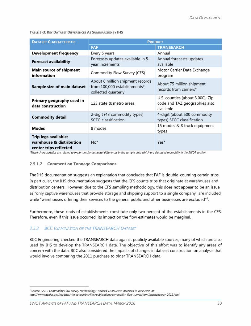
DATA DEVELOPMENT
SWOT ANALYSIS OF FAF AND TRANSEARCH DATA, MARCH 2016 30
TABLE 3-3: KEY DATASET DIFFERENCES AS SUMMARIZED BY IHS
DATASET CHARACTERISTIC PRODUCT
FAF TRANSEARCH
Development frequency Every 5 years Annual
Forecast availability Forecasts updates available in 5-
year increments
Annual forecasts updates
available
Main source of shipment
information Commodity Flow Survey (CFS)
Motor Carrier Data Exchange
program
Sample size of main dataset
About 6 million shipment records
from 100,000 establishments*;
collected quarterly
About 75 million shipment
records from carriers*
Primary geography used in
data construction 123 state & metro areas
U.S. counties (about 3,000); Zip
code and TAZ geographies also
available
Commodity detail 2-digit (43 commodity types)
SCTG classification
4-digit (about 500 commodity
types) STCC classification
Modes 8 modes 15 modes & 8 truck equipment
types
Trip legs available;
warehouse & distribution
center trips reflected
No* Yes*
*These characteristics are related to important fundamental differences in the sample data which are discussed more fully in the SWOT section
2.5.1.2 Comment on Tonnage Comparisons
The IHS documentation suggests an explanation that concludes that FAF is double-counting certain trips.
In particular, the IHS documentation suggests that the CFS counts trips that originate at warehouses and
distribution centers. However, due to the CFS sampling methodology, this does not appear to be an issue
as “only captive warehouses that provide storage and shipping support to a single company” are included
while “warehouses offering their services to the general public and other businesses are excluded”1.
Furthermore, these kinds of establishments constitute only two percent of the establishments in the CFS.
Therefore, even if this issue occurred, its impact on the flow estimates would be marginal.
2.5.2 BCC EXAMINATION OF THE TRANSEARCH DATASET
BCC Engineering checked the TRANSEARCH data against publicly available sources, many of which are also
used by IHS to develop the TRANSEARCH data. The objective of this effort was to identify any areas of
concern with the data. BCC also considered the impacts of changes in dataset construction on analysis that
would involve comparing the 2011 purchase to older TRANSEARCH data.
1 Source: “2012 Commodity Flow Survey Methodology” Revised 12/03/2014 accessed in June 2015 at:
http://www.rita.dot.gov/bts/sites/rita.dot.gov.bts/files/publications/commodity_flow_survey/html/methodology_2012.html
DATA DEVELOPMENT
SWOT ANALYSIS OF FAF AND TRANSEARCH DATA, MARCH 2016 31
2.5.2.1 Documentation of Underlying Data Sources
The construction of the TRANSEARCH dataset is detailed earlier in this report. Several of the underlying
data sources that are used to construct the TRANSEARCH data are reviewed by BCC. These include:
» The BTS border crossing data;
» The BTS T-100 air cargo dataset;
» The STB Carload Waybill sample;
» The EIA coal distribution data;
» Commodity Flow Survey statistics;
» County Business Patterns employment data;
» USDA crop production data;
» University of Florida’s Bureau of Economic and Business Research (BEBR) population projections for
Florida;
» Freight Analysis Framework;
» American Transportation Research Institute (ATRI; note: this was not a TRANSEARCH input);
» Gross Domestic Product (GDP);
» InfoGroup business data;
» Longitudinal Employer Household Dynamics;
» Mexico Economic Census;
» Army Corps of Engineers U.S. Waterway data; and
» Historical REEBIE and TRANSEARCH data.
The BCC report describes each dataset and its relevance to commodity flow projections.
2.5.2.2 TRANSEARCH QA/QC
Tonnages from the TRANSEARCH data were summarized across origins, destinations, and modes. The data
were then examined and compared to other sources.
The BCC report concluded that overall the 2011 TRANSEARCH database is a good source of information for
stakeholders across Florida. Additionally, the report concluded that the data development process is sound.
BCC also found the following concerns with the data:
» The growth rates in commodity flows decline in year 2020 (in comparison with years 2011 to 2020).
This impacts various areas of the dataset such as total flows in Santa Rosa County and in rail
tonnages.
» A decrease in commodity flow tonnage originations is predicted for Hernando County from 2011
to 2040 in spite of projected increases in population and destination traffic. BCC raised the question
of how the BEBR population projections are used for production and consumption estimates.
» Waterborne tonnages are projected to increase in TRANSEARCH, which is contrary to the trend
exhibited in the observed data and the FAF data.
» TRANSEARCH exhibits an increase in rail tonnages although rail tonnage declined in recent years.
» Rail tonnage in TRANSEARCH exceeds the Waybill sample and FAF3 forecast (through 2030), which
may be only partly explained by sample obfuscation.
DATA DEVELOPMENT
SWOT ANALYSIS OF FAF AND TRANSEARCH DATA, MARCH 2016 32
BCC suggested inquiring with IHS to determine possible explanations to these questions. BCC also
recommended further avenues of data exploration to provide additional insights into the TRANSEARCH
data:
» Examine correlation between the food/crop industry and population growth;
» Calculate growth in commodity flows by mode by county;
» Examine growth and decline in flows by commodity type; and
» Evaluate the predicted Panama Canal impact to determine if it is factored into the post-2020 flows.
2.5.2.3 Comparing the 2000 and 2011 TRANSEARCH Datasets
The TRANSEARCH data have undergone changes over the years. The IHS methodology report documents
the TRANSEARCH dataset development history. The most recent changes are documented in release notes
provided with the data purchase. The historical evolution of the data construction process, including recent
dataset adjustments, would likely have a notable impact on any analysis that involves comparisons of the
2011 data and historical data.
These changes could have two main impacts. First, since the 2011 TRANSEARCH dataset relied partly on
historical TRANSEARCH (and REEBIE) data for dataset construction, it is possible that erroneous trends from
previous years are reflected in the 2011 version. However, IHS has likely addressed any major known issues
already. Second, if the 2011 version is compared to the 2000 data (which is the FDOT’s last purchase prior
to the 2011 purchase), then differences in the underlying data or dataset construction may be interpreted
as differences in commodity flow patterns. Therefore, if this becomes a topic of interest, then it will be
important to consider changes in the underlying data when the analysis is conducted. In addition, as BCC
also noted, the historical data appears to have issues in tonnages by mode. Such concerns should be
examined in more detail if a 2000 vs. 2011 analysis is undertaken. Furthermore, a 1998 TRANSEARCH
(REEBIE) dataset was also noted in the BCC report
SWOT ANALYSIS OF FAF AND TRANSEARCH DATA, MARCH 2016 33
CHAPTER 3
SWOT ANALYSIS

SWOT ANALYSIS
SWOT ANALYSIS OF FAF AND TRANSEARCH DATA, MARCH 2016 34
INTENTIONALLY LEFT BLANK
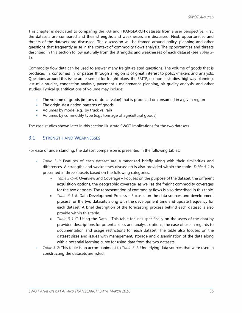
SWOT ANALYSIS
SWOT ANALYSIS OF FAF AND TRANSEARCH DATA, MARCH 2016 35
This chapter is dedicated to comparing the FAF and TRANSEARCH datasets from a user perspective. First,
the datasets are compared and their strengths and weaknesses are discussed. Next, opportunities and
threats of the datasets are discussed. The discussion will be framed around policy, planning and other
questions that frequently arise in the context of commodity flows analysis. The opportunities and threats
described in this section follow naturally from the strengths and weaknesses of each dataset (see Table 3-
1).
Commodity flow data can be used to answer many freight-related questions. The volume of goods that is
produced in, consumed in, or passes through a region is of great interest to policy-makers and analysts.
Questions around this issue are essential for freight plans, the FMTP, economic studies, highway planning,
last-mile studies, congestion analysis, pavement / maintenance planning, air quality analysis, and other
studies. Typical quantifications of volume may include:
» The volume of goods (in tons or dollar value) that is produced or consumed in a given region
» The origin-destination patterns of goods
» Volumes by mode (e.g., by truck vs. rail)
» Volumes by commodity type (e.g., tonnage of agricultural goods)
The case studies shown later in this section illustrate SWOT implications for the two datasets.
3.1 STRENGTH AND WEAKNESSES
For ease of understanding, the dataset comparison is presented in the following tables:
» Table 3-1: Features of each dataset are summarized briefly along with their similarities and
differences. A strengths and weaknesses discussion is also provided within the table. Table 4-1 is
presented in three subsets based on the following categories.
» Table 3-1-A: Overview and Coverage – Focuses on the purpose of the dataset, the different
acquisition options, the geographic coverage, as well as the freight commodity coverages
for the two datasets. The representation of commodity flows is also described in this table.
» Table 3-1-B: Data Development Process – Focuses on the data sources and development
process for the two datasets along with the development time and update frequency for
each dataset. A brief description of the forecasting process behind each dataset is also
provide within this table.
» Table 3-1-C: Using the Data – This table focuses specifically on the users of the data by
provided descriptions for potential uses and analysis options, the ease of use in regards to
documentation and usage restrictions for each dataset. The table also focuses on the
dataset sizes and issues with management, storage and dissemination of the data along
with a potential learning curve for using data from the two datasets.
» Table 3-2: This table is an accompaniment to Table 3-1. Underlying data sources that were used in
constructing the datasets are listed.

SWOT ANALYSIS
SWOT ANALYSIS OF FAF AND TRANSEARCH DATA, MARCH 2016 36
INTENTIONALLY LEFT BLANK
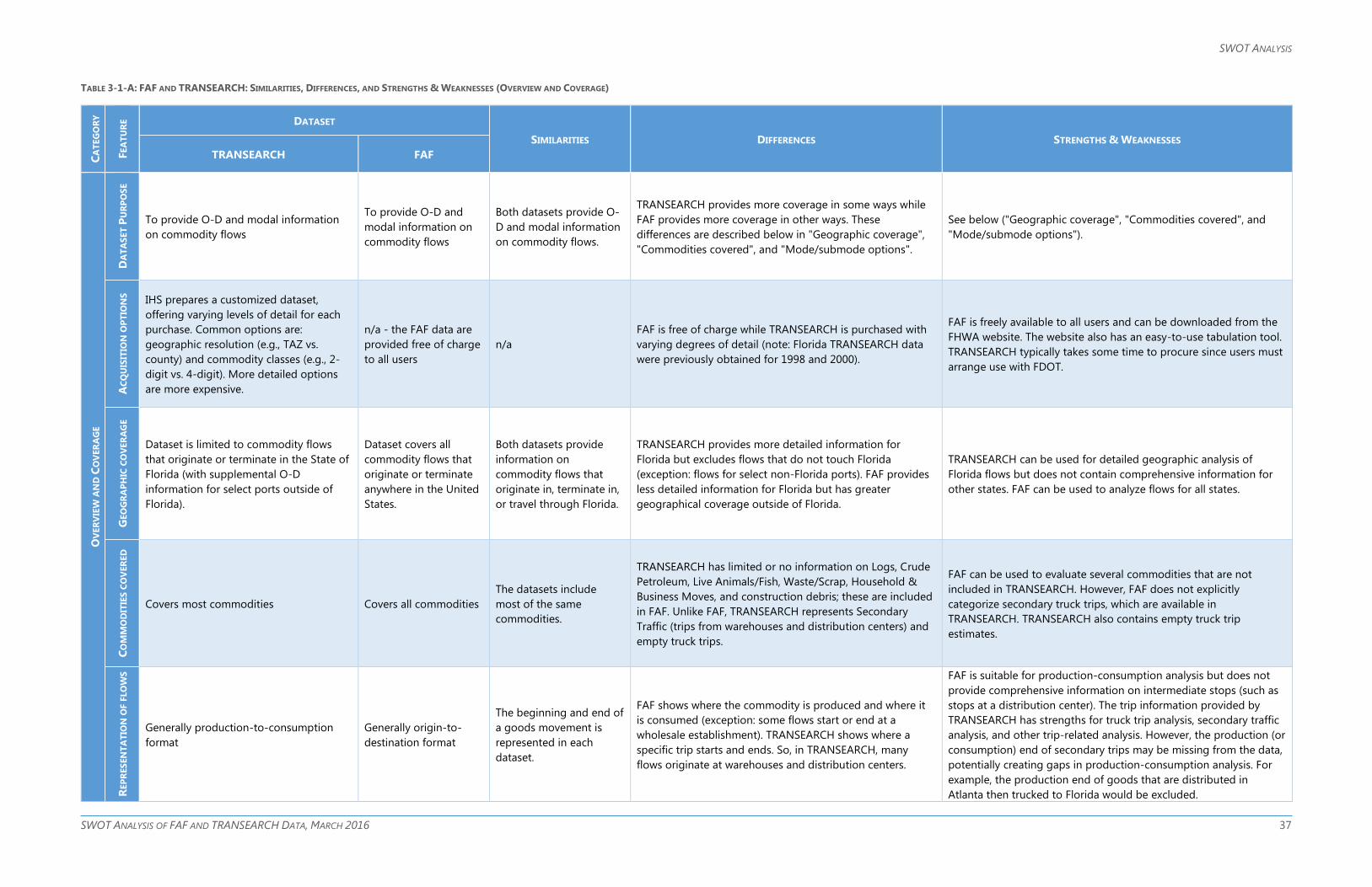
SWOT ANALYSIS
SWOT ANALYSIS OF FAF AND TRANSEARCH DATA, MARCH 2016 37
TABLE 3-1-A: FAF AND TRANSEARCH: SIMILARITIES, DIFFERENCES, AND STRENGTHS & WEAKNESSES (OVERVIEW AND COVERAGE) C
AT
EG
OR
Y
FEA
TU
RE
DATASET
SIMILARITIES DIFFERENCES STRENGTHS & WEAKNESSES
TRANSEARCH FAF
OV
ER
VIE
W A
ND
CO
VER
AG
E
DA
TA
SET
PU
RP
OS
E
To provide O-D and modal information
on commodity flows
To provide O-D and
modal information on
commodity flows
Both datasets provide O-
D and modal information
on commodity flows.
TRANSEARCH provides more coverage in some ways while
FAF provides more coverage in other ways. These
differences are described below in "Geographic coverage",
"Commodities covered", and "Mode/submode options".
See below ("Geographic coverage", "Commodities covered", and
"Mode/submode options").
AC
QU
ISIT
ION
OP
TIO
NS
IHS prepares a customized dataset,
offering varying levels of detail for each
purchase. Common options are:
geographic resolution (e.g., TAZ vs.
county) and commodity classes (e.g., 2-
digit vs. 4-digit). More detailed options
are more expensive.
n/a - the FAF data are
provided free of charge
to all users
n/a
FAF is free of charge while TRANSEARCH is purchased with
varying degrees of detail (note: Florida TRANSEARCH data
were previously obtained for 1998 and 2000).
FAF is freely available to all users and can be downloaded from the
FHWA website. The website also has an easy-to-use tabulation tool.
TRANSEARCH typically takes some time to procure since users must
arrange use with FDOT.
GEO
GR
AP
HIC
CO
VER
AG
E
Dataset is limited to commodity flows
that originate or terminate in the State of
Florida (with supplemental O-D
information for select ports outside of
Florida).
Dataset covers all
commodity flows that
originate or terminate
anywhere in the United
States.
Both datasets provide
information on
commodity flows that
originate in, terminate in,
or travel through Florida.
TRANSEARCH provides more detailed information for
Florida but excludes flows that do not touch Florida
(exception: flows for select non-Florida ports). FAF provides
less detailed information for Florida but has greater
geographical coverage outside of Florida.
TRANSEARCH can be used for detailed geographic analysis of
Florida flows but does not contain comprehensive information for
other states. FAF can be used to analyze flows for all states.
CO
MM
OD
ITIE
S C
OV
ER
ED
Covers most commodities Covers all commodities
The datasets include
most of the same
commodities.
TRANSEARCH has limited or no information on Logs, Crude
Petroleum, Live Animals/Fish, Waste/Scrap, Household &
Business Moves, and construction debris; these are included
in FAF. Unlike FAF, TRANSEARCH represents Secondary
Traffic (trips from warehouses and distribution centers) and
empty truck trips.
FAF can be used to evaluate several commodities that are not
included in TRANSEARCH. However, FAF does not explicitly
categorize secondary truck trips, which are available in
TRANSEARCH. TRANSEARCH also contains empty truck trip
estimates.
REP
RES
EN
TA
TIO
N O
F F
LO
WS
Generally production-to-consumption
format
Generally origin-to-
destination format
The beginning and end of
a goods movement is
represented in each
dataset.
FAF shows where the commodity is produced and where it
is consumed (exception: some flows start or end at a
wholesale establishment). TRANSEARCH shows where a
specific trip starts and ends. So, in TRANSEARCH, many
flows originate at warehouses and distribution centers.
FAF is suitable for production-consumption analysis but does not
provide comprehensive information on intermediate stops (such as
stops at a distribution center). The trip information provided by
TRANSEARCH has strengths for truck trip analysis, secondary traffic
analysis, and other trip-related analysis. However, the production (or
consumption) end of secondary trips may be missing from the data,
potentially creating gaps in production-consumption analysis. For
example, the production end of goods that are distributed in
Atlanta then trucked to Florida would be excluded.

SWOT ANALYSIS
SWOT ANALYSIS OF FAF AND TRANSEARCH DATA, MARCH 2016 38
TABLE 3-1-B: FAF AND TRANSEARCH: SIMILARITIES, DIFFERENCES, AND STRENGTHS & WEAKNESSES (DATA DEVELOPMENT PROCESS) C
AT
EG
OR
Y
FEA
TU
RE
DATASET
SIMILARITIES DIFFERENCES STRENGTHS & WEAKNESSES
TRANSEARCH FAF
DA
TA
SET
DEV
ELO
PM
EN
T P
RO
CES
SES
DA
TA
SO
UR
CES
See Table 3-2. The main sources are
proprietary economic models and truck
carrier data.
See Table 3-2. The main
source is the CFS.
Many of the same
sources are used
Key differences: TRANSEARCH relies more heavily on the
Motor Carrier Data Exchange Program and propriety
economic models. FAF relies mainly on the Commodity Flow
Survey.
TRANSEARCH may be advantageous for evaluating individual trips,
especially truck trips. FAF may be advantageous for evaluating the
"chained" trip from a production-to-consumption perspective. It is
important to note that TRANSEARCH also contains production-
consumption data.
DA
TA
DEV
ELO
PM
EN
T P
RO
CES
S
See Chapter 2. IHS' economic BMI
models generate production and
consumption information; O-D patterns
are determined mainly using carrier data;
and other sources are used to
supplement other commodities and
modes.
See Chapter 2. CFS data
are supplemented with
models to fill in O-D
gaps plus estimation of
flows for commodities
that are not covered in
the CFS scope.
Both databases
fundamentally try to
reflect the activities of
companies that generate
(or consume) commodity
shipments.
Business activity is captured more through economic
models in TRANSEARCH and through shipping surveys in
FAF.
While the data construction approaches have some major
differences, the assessment of the overall strength of each approach
requires more evaluation.
DA
TA
DEV
ELO
PM
EN
T T
IME
Approximately 3 months - 2 years
depending on level of detail requested Approximately 3 years
Both datasets present
historical data; neither is
"real-time"
TRANSEARCH has a faster preparation time.
TRANSEARCH's faster preparation time should improve its
representation of current freight flows. A longer time lag in
development may decrease the accuracy of the data due to
fluctuations in economic cycles.
UP
DA
TE F
REQ
UEN
CY
Annual
Every five years with
provisional estimates
for the current year
Updates occur on a
regular basis TRANSEARCH is updated more frequently
While more regular updates typically provide more up-to-date
information, TRANSEARCH updates must be purchased. In contrast,
FAF data are updated less frequently but the updates are free.
FO
REC
AS
TIN
G P
RO
CES
S
See Chapter 2. Freight supply and
demand is forecast at the county level
using the BMI models; projected national
and global economic trends are used as
control totals. A range of forecasts was
developed for the 2011 purchase.
See Chapter 2.
Projected national and
global economic trends
are used.
Projected national and
global economic trends
are used.
TRANSEARCH includes more distinctions in freight forecasts
at the county level. The 2011 TRANSEARCH data also
includes high-medium-low estimates based on economic
alternatives.
The TRANSEARCH forecasting process is consistent with the
theoretical foundation of the base year construction process (i.e.,
the use of the BMI models for both processes). Since the CFS is not
available for future years, FAF relies more on a factoring approach.
The high-medium-low ranges provided by TRANSEARCH provide
the user with more evaluation options.

SWOT ANALYSIS
SWOT ANALYSIS OF FAF AND TRANSEARCH DATA, MARCH 2016 39
TABLE 3-1-C: FAF AND TRANSEARCH: SIMILARITIES, DIFFERENCES, AND STRENGTHS & WEAKNESSES (USING THE DATA) C
AT
EG
OR
Y
FEA
TU
RE
DATASET
SIMILARITIES DIFFERENCES STRENGTHS & WEAKNESSES
TRANSEARCH FAF
US
ING
TH
E D
AT
A
PO
TEN
TIA
L U
SES
&
AN
ALY
SIS
OP
TIO
NS
Tons, value and units (e.g., number of
trucks) of goods that originate in,
terminate in, or flow between zones;
Includes assignment information (volume
estimates) for the highway and rail
networks.
Tons and value of goods
that originate in,
terminate in, or flow
between zones; Includes
assignment information
(volume estimates) for
the highway network.
Tons and value of goods that
originate in, terminate in, or flow
between zones; Highway
assignment information.
TRANSEARCH also includes units and
rail assignment information.
FAF is well suited for interstate analysis. Limited geographic detail
and potential sample size limitations in FAF make it less suited for
intra-Florida analysis. TRANSEARCH is well suited for detailed
analysis of trips that begin or end in Florida. The availability of units
(e.g., number of trucks) and a rail assignment are TRANSEARCH
analysis options that are unavailable in FAF without additional
analysis by the user.
PO
TEN
TIA
L
US
ER
S Types of users: GIS analysts, policy makers,
modelers, operations analysts, economists,
and others in public sector agencies,
private sector researchers, and academia
(Same) Same types of users n/a n/a
EA
SE O
F U
SE:
US
AG
E
RES
TR
ICT
ION
S Users must first get approval from FDOT.
The default version has limited rail
information - those who want to use the
Waybill-enhanced version must also get
permission from the STB. Usage
restrictions must be observed.
No restrictions.
Both are readily available to
FDOT staff and consultants who
work on FDOT projects.
TRANSEARCH has restrictions on who
can use it and how the data can be
published given its confidential nature.
Usage of FAF is unrestricted. TRANSEARCH users must adhere to
restrictions on use or publication of the data as described in the
licensing agreement.
EA
SE O
F U
SE:
CO
MP
REH
EN
SIV
EN
ES
S
OF D
OC
UM
EN
TA
TIO
N
Documentation is very thorough. Documentation is very
thorough.
The documentation is of similar
quality and completeness. n/a n/a
PO
TEN
TIA
L
US
ER
S
FDOT has contracted with IHS to provide
technical support.
The FHWA or other
developers may be able
to assist with answering
some questions.
Technical support and a
community of users are options
for assistance with both
products.
Since IHS is under contract to FDOT,
TRANSEARCH users might be able to
procure greater assistance from IHS.
Users have good options for support, whether from the user
community or from Global Insight representatives.
EA
SE O
F U
SE:
DA
TA
SET
SIZ
E
The Access database is about 1.5 GB. The Access version is
about 230 MB.
Both datasets are large, but
manageable with most
computers.
The TRANSEARCH data, which is six
times larger than FAF, may require
longer processing times on older
computers.
FAF's smaller size makes it faster to process and analyze, but both
datasets can be analyzed in reasonable timeframes using modern
computers.
EA
SE O
F U
SE:
MA
NA
GEM
EN
T,
ST
OR
AG
E A
ND
DIS
SEM
INA
TIO
N
OF T
HE D
AT
A
Due to proprietary restrictions, FDOT must
assign staff resources to manage the
dissemination of the data.
The data are readily
available online, so this is
not an issue with FAF.
n/a
TRANSEARCH storage and
dissemination requires management
from FDOT staff. FAF requires no FDOT
resources.
TRANSEARCH licensing requirements effectively require FDOT staff
to devote some time to disseminating the data and/or managing its
use. Usage of FAF does not require this kind of oversight since FAF
does not have restrictions on use or dissemination.
EA
SE O
F
US
E:
LEA
RN
ING
CU
RV
E
The learning curve is comparable for each. The learning curve is
comparable for each.
The learning curve is
comparable for each. n/a n/a

SWOT ANALYSIS
SWOT ANALYSIS OF FAF AND TRANSEARCH DATA, MARCH 2016 40
INTENTIONALLY LEFT BLANK
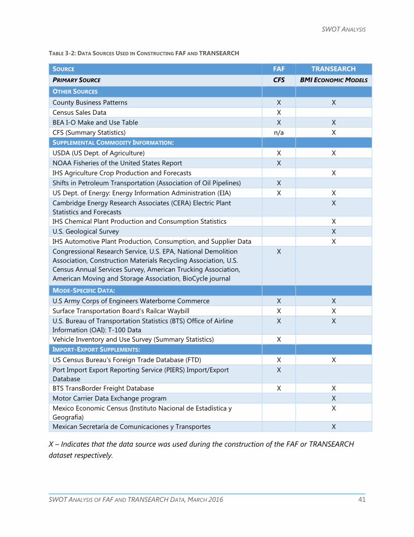
SWOT ANALYSIS
SWOT ANALYSIS OF FAF AND TRANSEARCH DATA, MARCH 2016 41
TABLE 3-2: DATA SOURCES USED IN CONSTRUCTING FAF AND TRANSEARCH
SOURCE FAF TRANSEARCH
PRIMARY SOURCE CFS BMI ECONOMIC MODELS
OTHER SOURCES
County Business Patterns X X
Census Sales Data X
BEA I-O Make and Use Table X X
CFS (Summary Statistics) n/a X
SUPPLEMENTAL COMMODITY INFORMATION:
USDA (US Dept. of Agriculture) X X
NOAA Fisheries of the United States Report X
IHS Agriculture Crop Production and Forecasts X
Shifts in Petroleum Transportation (Association of Oil Pipelines) X
US Dept. of Energy: Energy Information Administration (EIA) X X
Cambridge Energy Research Associates (CERA) Electric Plant
Statistics and Forecasts
X
IHS Chemical Plant Production and Consumption Statistics X
U.S. Geological Survey X
IHS Automotive Plant Production, Consumption, and Supplier Data X
Congressional Research Service, U.S. EPA, National Demolition
Association, Construction Materials Recycling Association, U.S.
Census Annual Services Survey, American Trucking Association,
American Moving and Storage Association, BioCycle journal
X
MODE-SPECIFIC DATA:
U.S Army Corps of Engineers Waterborne Commerce X X
Surface Transportation Board’s Railcar Waybill X X
U.S. Bureau of Transportation Statistics (BTS) Office of Airline
Information (OAI): T-100 Data
X X
Vehicle Inventory and Use Survey (Summary Statistics) X
IMPORT-EXPORT SUPPLEMENTS:
US Census Bureau’s Foreign Trade Database (FTD) X X
Port Import Export Reporting Service (PIERS) Import/Export
Database
X
BTS TransBorder Freight Database X X
Motor Carrier Data Exchange program X
Mexico Economic Census (Instituto Nacional de Estadística y
Geografía)
X
Mexican Secretaría de Comunicaciones y Transportes X
X – Indicates that the data source was used during the construction of the FAF or TRANSEARCH
dataset respectively.
SWOT ANALYSIS
SWOT ANALYSIS OF FAF AND TRANSEARCH DATA, MARCH 2016 42
3.2 OPPORTUNITIES
While both FAF and TRANSEARCH can be used to answer the same types of questions, the datasets offer
different opportunities in terms of the level of detail that can be used to answer questions. In most ways,
TRANSEARCH presents more opportunities for analysis of commodities in Florida while FAF presents more
opportunities for analysis throughout the U.S. This difference in application options occurs because the
datasets contain different levels of resolution in regards to commodity type, geographic resolution and
modal information.
Generally speaking, the Florida TRANSEARCH data product allows the user the opportunity to summarize
commodity flows over a wide range of geographies, commodities, and modes throughout Florida. The
dataset is extremely detailed in terms of geographic resolution (about 8,500 TAZs in Florida), commodity
resolution (hundreds of categories are delineated), and modal detail (it includes rail, air, water and truck
modes plus equipment type for truck). Therefore, TRANSEARCH offers the user the capability to evaluate
commodity flow questions down to the TAZ level for any mode and commodity in the dataset. The data
can be aggregated to the municipal, MPO, county, district or other level as needed as long as the area of
interest is within Florida (or in the included nearby areas in Alabama and Georgia). TRANSEARCH flows can
be studies at the 4-digit STCC level or aggregated to a higher level. Similarly, the flows can be studies based
on the detailed mode and equipment type information or it can be summarized at an aggregate level.
FAF, on the other hand, has only five zones in the State of Florida and contains less commodity and modal
detail than TRANSEARCH. As the case studies below illustrate, the FAF zones do not nest exactly with
Florida districts, although they are comparable in size to the average district. Therefore, by default the FAF
data can be used for analyzing flows for the state in its entirety or for a sub-region within the state based
on the FAF zonal boundaries.
While FAF is less detailed than TRANSEARCH in Florida, FAF contains more information for the rest of the
U.S. The Florida TRANSEARCH purchase only contains flows that touch Florida (plus some area on its
northern edges and a select sample of non-Florida ports). For users that need to evaluate other flows, FAF
is the better option. For example, a user might want to compare flows of manufactured products in
Florida vs. other southern states. TRANSEARCH contains comprehensive information for Florida only while
FAF contains similar information for all states of interest.
It is important to understand the difference between commodity coverage and commodity resolution. The
TRANSEARCH data has very detailed commodity resolution, meaning that there are hundreds of different
categories of commodities. On the other hand, while FAF has only about 40 commodity categories, it covers
more commodities than TRANSEARCH. For example, Crude Petroleum is covered in FAF but not in
TRANSEARCH – as a result, FAF is the main option for evaluating Crude Petroleum flows. Copper Ore, Lead
Ore, Zinc Ore and other ores are differentiated in TRANSEARCH while all Metallic Ores are grouped in a
single commodity category in FAF. As a result, studying all metallic ores in aggregate can be accomplished
using either dataset. But if the user wants to evaluate a specific ore, then TRANSEARCH presents more
opportunities for analysis. Appendix A provides the detailed commodity classes for FAF and TRANSEARCH
databases.
SWOT ANALYSIS
SWOT ANALYSIS OF FAF AND TRANSEARCH DATA, MARCH 2016 43
3.3 THREATS
One of the main “threats” of commodity flows analysis relates to the accuracy of the data and the potential
to treat the flow estimates as factual information. Both datasets have major sources of uncertainty that can
impact the accuracy of analysis, including:
» The use of data samples to develop commodity flow estimates:
» The FAF dataset is built primarily using the CFS, which samples about one in seven
businesses and gathers shipment information for about four weeks of the year from each
business. The CFS is administered every five years. Therefore, major changes in the
economy could impact the accuracy of the flow estimates.
» The TRANSEARCH dataset relies heavily on the Motor Carrier Program survey data, which
annually samples about four percent of all dry van traffic based on 22 carriers. The sample
consists predominantly of longer distance hauls by large carriers with lower rates of
shorter-distance trips and less participation by smaller carriers. One possible implication
for analysis is that the truck flow estimates may be more accurate for long-distance flows
than for intra-state movements.
» For both data samples, various sectors or geographic areas could be relatively under-
sampled or missing. This reduces the level of confidence in the flow estimates.
» The use of models to develop commodity flow estimates:
» Both data construction efforts use modeling processes to enhance the flow estimates. The
objective in both instances is to add value for the user. The TRANSEARCH estimates are
developed first at the county level using the company’s proprietary BMI models. The FAF
data construction process uses statistical processes (iterative proportional fitting and log-
linear modeling) to estimate values for O-D pairs for which information was missing or
unavailable in the CFS sample.
» While these practices ultimately allow the end user to conduct analysis at a more detailed
level, the user must remember that uncertainty is an inherent feature in any model. Just as
modeling output is presented as an estimate, it is good practice to treat the results of
commodity flows analysis as an estimate.
» The use of alternative methods to expand the flow estimates:
» The main FAF and TRANSEARCH data sample and modeling processes do not account for
numerous commodity types such as coal and crops. Estimates on these flows were
developed using a mix of data, models, factors, and judgment. Uncertainty is inherent in all
of these elements.
3.4 SUMMARY OF SWOT ANALYSIS
Overall, while more information means more analysis opportunities, understanding the limitations of the
data is critical. The user must remember that more information does not necessarily equal greater accuracy.
More detail can also make it more difficult to check and verify findings. A certain amount of caution is
helpful both when conducting analysis and conveying results to others, such as an audience of policy-
makers.

SWOT ANALYSIS
SWOT ANALYSIS OF FAF AND TRANSEARCH DATA, MARCH 2016 44
INTENTIONALLY LEFT BLANK
SWOT ANALYSIS OF FAF AND TRANSEARCH DATA, MARCH 2016 45
CHAPTER 4
USER GUIDANCE

USER GUIDANCE
SWOT ANALYSIS OF FAF AND TRANSEARCH DATA, MARCH 2016 46
INTENTIONALLY LEFT BLANK
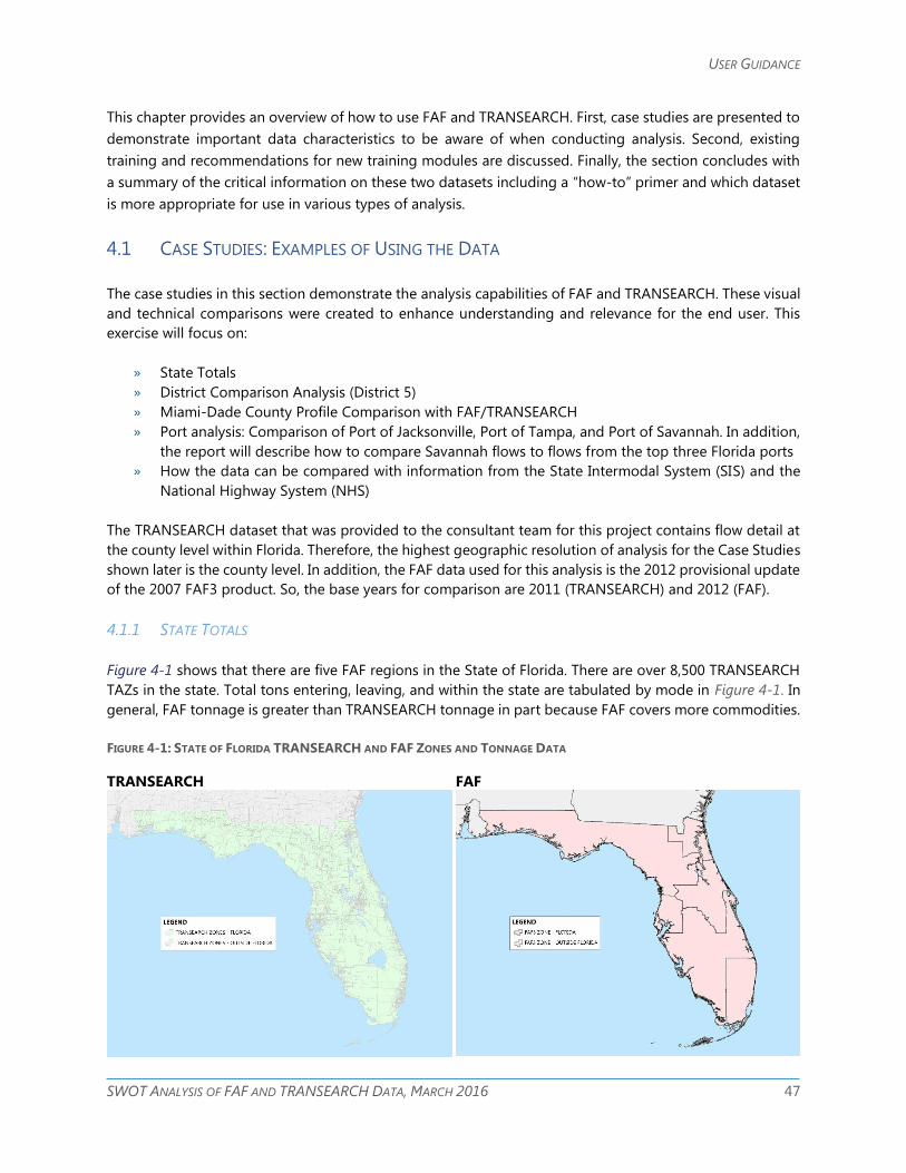
USER GUIDANCE
SWOT ANALYSIS OF FAF AND TRANSEARCH DATA, MARCH 2016 47
This chapter provides an overview of how to use FAF and TRANSEARCH. First, case studies are presented to
demonstrate important data characteristics to be aware of when conducting analysis. Second, existing
training and recommendations for new training modules are discussed. Finally, the section concludes with
a summary of the critical information on these two datasets including a “how-to” primer and which dataset
is more appropriate for use in various types of analysis.
4.1 CASE STUDIES: EXAMPLES OF USING THE DATA
The case studies in this section demonstrate the analysis capabilities of FAF and TRANSEARCH. These visual
and technical comparisons were created to enhance understanding and relevance for the end user. This
exercise will focus on:
» State Totals
» District Comparison Analysis (District 5)
» Miami-Dade County Profile Comparison with FAF/TRANSEARCH
» Port analysis: Comparison of Port of Jacksonville, Port of Tampa, and Port of Savannah. In addition,
the report will describe how to compare Savannah flows to flows from the top three Florida ports
» How the data can be compared with information from the State Intermodal System (SIS) and the
National Highway System (NHS)
The TRANSEARCH dataset that was provided to the consultant team for this project contains flow detail at
the county level within Florida. Therefore, the highest geographic resolution of analysis for the Case Studies
shown later is the county level. In addition, the FAF data used for this analysis is the 2012 provisional update
of the 2007 FAF3 product. So, the base years for comparison are 2011 (TRANSEARCH) and 2012 (FAF).
4.1.1 STATE TOTALS
Figure 4-1 shows that there are five FAF regions in the State of Florida. There are over 8,500 TRANSEARCH
TAZs in the state. Total tons entering, leaving, and within the state are tabulated by mode in Figure 4-1. In
general, FAF tonnage is greater than TRANSEARCH tonnage in part because FAF covers more commodities.
FIGURE 4-1: STATE OF FLORIDA TRANSEARCH AND FAF ZONES AND TONNAGE DATA
TRANSEARCH FAF

USER GUIDANCE
SWOT ANALYSIS OF FAF AND TRANSEARCH DATA, MARCH 2016 48
FIGURE 4-1: STATE OF FLORIDA TRANSEARCH AND FAF ZONES AND TONNAGE DATA CONTINUED…
TRANSEARCH DATA
MODE OF TRANSPORTATION
TOTAL FLORIDA TONS
TOTAL ENTERING
FLORIDA
LEAVING
FLORIDA
WITHIN
FLORIDA
SUM SUM SUM
Truck
Truck Truckload 51,139,719 26,470,052 101,799,240 179,409,011
Truck L-T-L 3,038,374 891,725 1,355,109 5,285,208
Truck PVT 23,014,337 15,121,543 90,100,276 128,236,156
Truck NEC 872,364 975,590 0 1,847,954
Subtotal 78,064,795 43,458,910 193,254,625 314,778,329
Rail Rail NEC 1,483,863 1,166,487 0 2,650,350
Subtotal 1,483,863 1,166,487 0 2,650,350
Water Water 44,775,218 5,114,063 1,068,575 50,957,856
Subtotal 44,775,218 5,114,063 1,068,575 50,957,856
Air Air 156,423 79,010 3,532 238,965
Subtotal 156,423 79,010 3,532 238,965
Oth
er
and
Un
kno
wn
Foreign Trade
Zones 520 0 0 520
Other 1,043 1,307 0 2,350
Subtotal 1,563 1,307 0 2,870
Total, All Modes 124,481,862 49,819,777 194,326,731 368,628,370
FAF DATA
MODE OF TRANSPORTATION
TOTAL FLORIDA TONS
TOTAL ENTERING
FLORIDA
LEAVING
FLORIDA
WITHIN
FLORIDA
SUM SUM SUM
Truck 71,833,827 48,177,106 694,300,485 814,311,419
Rail 41,472,840 11,193,638 18,520,171 71,186,649
Water 18,874,256 3,959,847 59,873 22,893,976
Air (incl. Truck-Air) 203,762 100,157 2,023 305,941
Multiple Modes & Mail 18,510,302 19,191,445 9,151,560 46,853,307
Pipeline 23,525,731 338,185 410,886 24,274,801
Other and Unknown 1,653,256 1,496,387 8,257,061 11,406,703
Total, All Modes 176,073,973 84,456,766 730,702,058 991,232,797
4.1.2 DISTRICT FIVE ANALYSIS
Figure 4-2 shows that the TRANSEARCH zones can be summarized for the District Five boundaries. The
Orlando area FAF zone is comparable to District Five but does not match the boundaries exactly. The FAF
zone is smaller than District Five. Total tons entering, leaving, and within the area are tabulated by mode in
Figure 4-2.
The next example, Miami-Dade County, shows how geographic differences in zonal structure can be
addressed to develop refined estimates. However, as the SWOT discussion emphasizes, the data may be
less accurate at these more detailed levels.
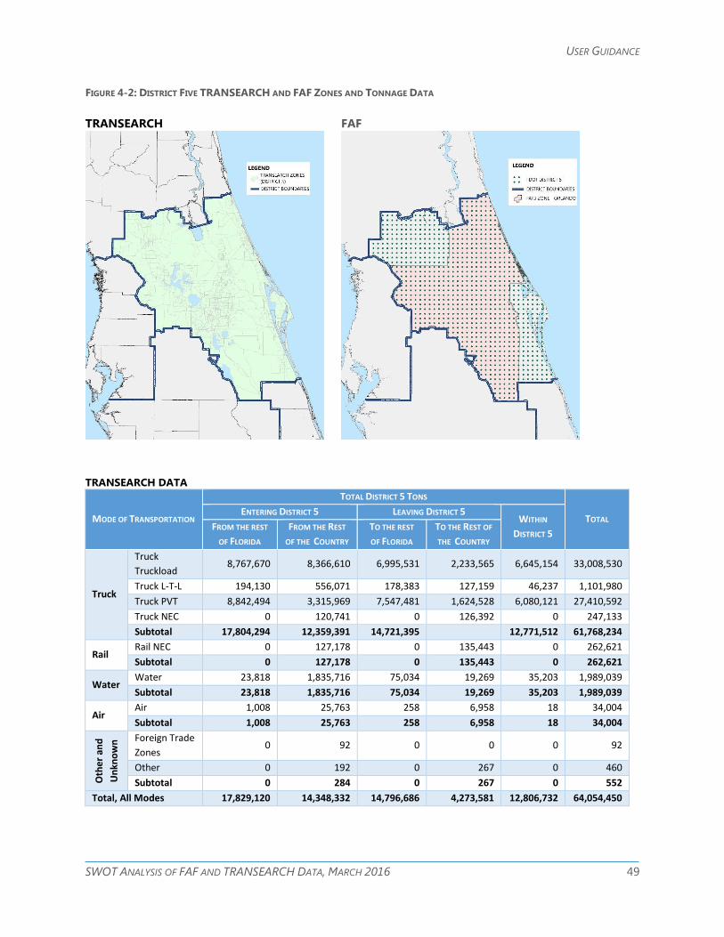
USER GUIDANCE
SWOT ANALYSIS OF FAF AND TRANSEARCH DATA, MARCH 2016 49
FIGURE 4-2: DISTRICT FIVE TRANSEARCH AND FAF ZONES AND TONNAGE DATA
TRANSEARCH FAF
TRANSEARCH DATA
MODE OF TRANSPORTATION
TOTAL DISTRICT 5 TONS
TOTAL ENTERING DISTRICT 5 LEAVING DISTRICT 5
WITHIN
DISTRICT 5 FROM THE REST
OF FLORIDA
FROM THE REST
OF THE COUNTRY
TO THE REST
OF FLORIDA
TO THE REST OF
THE COUNTRY
Truck
Truck
Truckload 8,767,670 8,366,610 6,995,531 2,233,565 6,645,154 33,008,530
Truck L-T-L 194,130 556,071 178,383 127,159 46,237 1,101,980
Truck PVT 8,842,494 3,315,969 7,547,481 1,624,528 6,080,121 27,410,592
Truck NEC 0 120,741 0 126,392 0 247,133
Subtotal 17,804,294 12,359,391 14,721,395 12,771,512 61,768,234
Rail Rail NEC 0 127,178 0 135,443 0 262,621
Subtotal 0 127,178 0 135,443 0 262,621
Water Water 23,818 1,835,716 75,034 19,269 35,203 1,989,039
Subtotal 23,818 1,835,716 75,034 19,269 35,203 1,989,039
Air Air 1,008 25,763 258 6,958 18 34,004
Subtotal 1,008 25,763 258 6,958 18 34,004
Oth
er
and
Un
kno
wn
Foreign Trade
Zones 0 92 0 0 0 92
Other 0 192 0 267 0 460
Subtotal 0 284 0 267 0 552
Total, All Modes 17,829,120 14,348,332 14,796,686 4,273,581 12,806,732 64,054,450
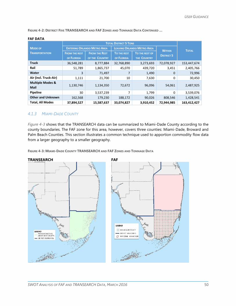
USER GUIDANCE
SWOT ANALYSIS OF FAF AND TRANSEARCH DATA, MARCH 2016 50
FIGURE 4-2: DISTRICT FIVE TRANSEARCH AND FAF ZONES AND TONNAGE DATA CONTINUED …
FAF DATA
MODE OF
TRANSPORTATION
TOTAL DISTRICT 5 TONS
TOTAL ENTERING ORLANDO METRO AREA LEAVING ORLANDO METRO AREA
WITHIN
DISTRICT 5 FROM THE REST
OF FLORIDA
FROM THE REST
OF THE COUNTRY
TO THE REST
OF FLORIDA
TO THE REST OF
THE COUNTRY
Truck 36,548,281 8,777,884 32,768,890 3,273,693 72,078,927 153,447,674
Rail 51,789 1,865,737 45,070 439,720 3,451 2,405,766
Water 3 71,497 7 1,490 0 72,996
Air (incl. Truck-Air) 1,111 21,700 10 7,630 0 30,450
Multiple Modes &
Mail 1,130,746 1,134,350 72,672 96,096 54,061 2,487,925
Pipeline 30 3,537,239 7 1,799 0 3,539,076
Other and Unknown 162,568 179,230 188,172 90,026 808,546 1,428,541
Total, All Modes 37,894,527 15,587,637 33,074,827 3,910,452 72,944,985 163,412,427
4.1.3 MIAMI-DADE COUNTY
Figure 4-3 shows that the TRANSEARCH data can be summarized to Miami-Dade County according to the
county boundaries. The FAF zone for this area, however, covers three counties: Miami-Dade, Broward and
Palm Beach Counties. This section illustrates a common technique used to apportion commodity flow data
from a larger geography to a smaller geography.
FIGURE 4-3: MIAMI-DADE COUNTY TRANSEARCH AND FAF ZONES AND TONNAGE DATA
TRANSEARCH FAF
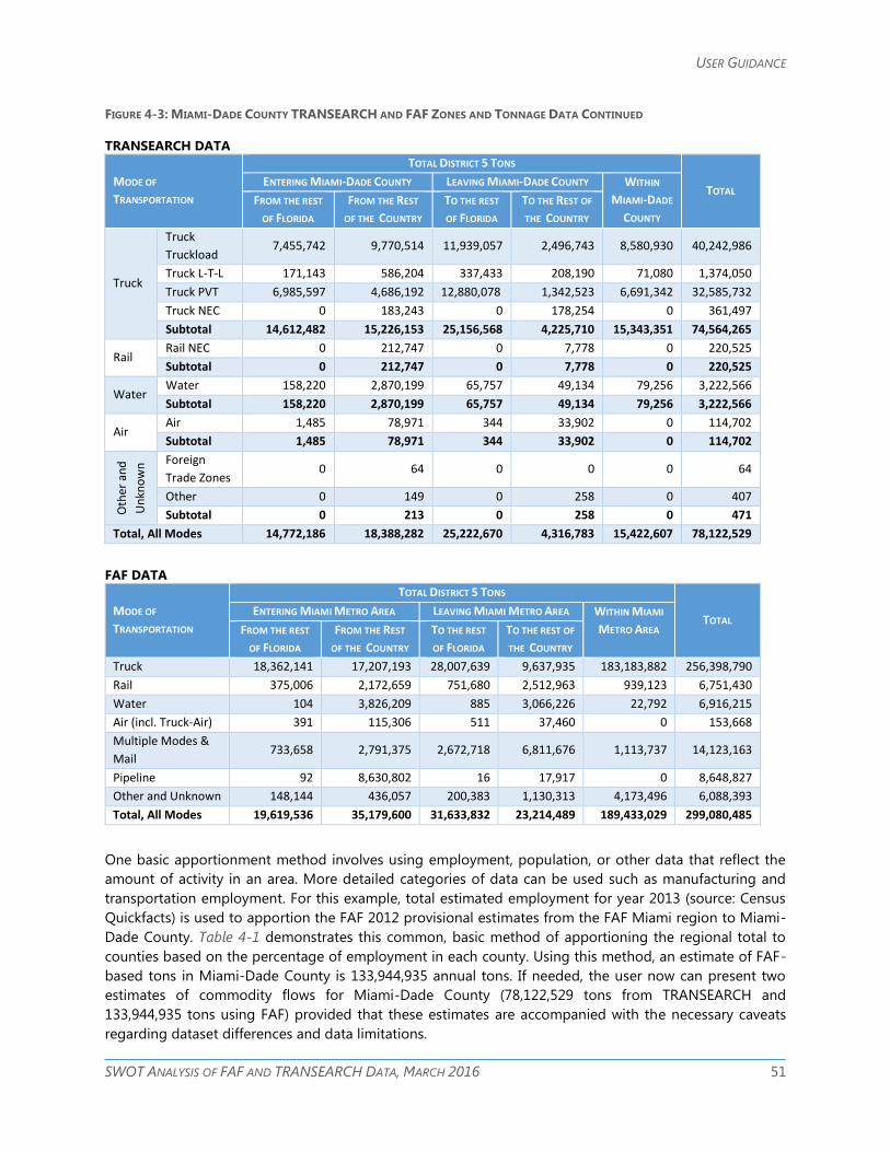
USER GUIDANCE
SWOT ANALYSIS OF FAF AND TRANSEARCH DATA, MARCH 2016 51
FIGURE 4-3: MIAMI-DADE COUNTY TRANSEARCH AND FAF ZONES AND TONNAGE DATA CONTINUED
TRANSEARCH DATA
MODE OF
TRANSPORTATION
TOTAL DISTRICT 5 TONS
TOTAL ENTERING MIAMI-DADE COUNTY LEAVING MIAMI-DADE COUNTY WITHIN
MIAMI-DADE
COUNTY
FROM THE REST
OF FLORIDA
FROM THE REST
OF THE COUNTRY
TO THE REST
OF FLORIDA
TO THE REST OF
THE COUNTRY
Truck
Truck
Truckload 7,455,742 9,770,514 11,939,057 2,496,743 8,580,930 40,242,986
Truck L-T-L 171,143 586,204 337,433 208,190 71,080 1,374,050
Truck PVT 6,985,597 4,686,192 12,880,078 1,342,523 6,691,342 32,585,732
Truck NEC 0 183,243 0 178,254 0 361,497
Subtotal 14,612,482 15,226,153 25,156,568 4,225,710 15,343,351 74,564,265
Rail Rail NEC 0 212,747 0 7,778 0 220,525
Subtotal 0 212,747 0 7,778 0 220,525
Water Water 158,220 2,870,199 65,757 49,134 79,256 3,222,566
Subtotal 158,220 2,870,199 65,757 49,134 79,256 3,222,566
Air Air 1,485 78,971 344 33,902 0 114,702
Subtotal 1,485 78,971 344 33,902 0 114,702
Oth
er a
nd
Un
kno
wn
Foreign
Trade Zones 0 64 0 0 0 64
Other 0 149 0 258 0 407
Subtotal 0 213 0 258 0 471
Total, All Modes 14,772,186 18,388,282 25,222,670 4,316,783 15,422,607 78,122,529
FAF DATA
MODE OF
TRANSPORTATION
TOTAL DISTRICT 5 TONS
TOTAL ENTERING MIAMI METRO AREA LEAVING MIAMI METRO AREA WITHIN MIAMI
METRO AREA
FROM THE REST
OF FLORIDA
FROM THE REST
OF THE COUNTRY
TO THE REST
OF FLORIDA
TO THE REST OF
THE COUNTRY
Truck 18,362,141 17,207,193 28,007,639 9,637,935 183,183,882 256,398,790
Rail 375,006 2,172,659 751,680 2,512,963 939,123 6,751,430
Water 104 3,826,209 885 3,066,226 22,792 6,916,215
Air (incl. Truck-Air) 391 115,306 511 37,460 0 153,668
Multiple Modes &
Mail 733,658 2,791,375 2,672,718 6,811,676 1,113,737 14,123,163
Pipeline 92 8,630,802 16 17,917 0 8,648,827
Other and Unknown 148,144 436,057 200,383 1,130,313 4,173,496 6,088,393
Total, All Modes 19,619,536 35,179,600 31,633,832 23,214,489 189,433,029 299,080,485
One basic apportionment method involves using employment, population, or other data that reflect the
amount of activity in an area. More detailed categories of data can be used such as manufacturing and
transportation employment. For this example, total estimated employment for year 2013 (source: Census
Quickfacts) is used to apportion the FAF 2012 provisional estimates from the FAF Miami region to Miami-
Dade County. Table 4-1 demonstrates this common, basic method of apportioning the regional total to
counties based on the percentage of employment in each county. Using this method, an estimate of FAF-
based tons in Miami-Dade County is 133,944,935 annual tons. If needed, the user now can present two
estimates of commodity flows for Miami-Dade County (78,122,529 tons from TRANSEARCH and
133,944,935 tons using FAF) provided that these estimates are accompanied with the necessary caveats
regarding dataset differences and data limitations.
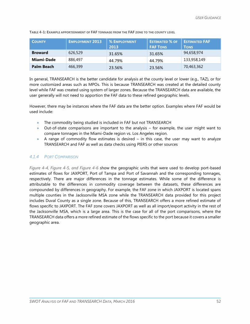
USER GUIDANCE
SWOT ANALYSIS OF FAF AND TRANSEARCH DATA, MARCH 2016 52
TABLE 4-1: EXAMPLE APPORTIONMENT OF FAF TONNAGE FROM THE FAF ZONE TO THE COUNTY LEVEL
COUNTY EMPLOYMENT 2013 % EMPLOYMENT
2013
ESTIMATED % OF
FAF TONS
ESTIMATED FAF
TONS
Broward 626,529 31.65% 31.65% 94,658,974
Miami-Dade 886,497 44.79% 44.79% 133,958,149
Palm Beach 466,399 23.56% 23.56% 70,463,362
In general, TRANSEARCH is the better candidate for analysis at the county level or lower (e.g., TAZ), or for
more customized areas such as MPOs. This is because TRANSEARCH was created at the detailed county
level while FAF was created using system of larger zones. Because the TRANSEARCH data are available, the
user generally will not need to apportion the FAF data to these refined geographic levels.
However, there may be instances where the FAF data are the better option. Examples where FAF would be
used include:
» The commodity being studied is included in FAF but not TRANSEARCH
» Out-of-state comparisons are important to the analysis – for example, the user might want to
compare tonnages in the Miami-Dade region vs. Los Angeles region.
» A range of commodity flow estimates is desired – in this case, the user may want to analyze
TRANSEARCH and FAF as well as data checks using PIERS or other sources
4.1.4 PORT COMPARISON
Figure 4-4, Figure 4-5, and Figure 4-6 show the geographic units that were used to develop port-based
estimates of flows for JAXPORT, Port of Tampa and Port of Savannah and the corresponding tonnages,
respectively. There are major differences in the tonnage estimates. While some of the difference is
attributable to the differences in commodity coverage between the datasets, these differences are
compounded by differences in geography. For example, the FAF zone in which JAXPORT is located spans
multiple counties in the Jacksonville MSA zone while the TRANSEARCH data provided for this project
includes Duval County as a single zone. Because of this, TRANSEARCH offers a more refined estimate of
flows specific to JAXPORT. The FAF zone covers JAXPORT as well as all import/export activity in the rest of
the Jacksonville MSA, which is a large area. This is the case for all of the port comparisons, where the
TRANSEARCH data offers a more refined estimate of the flows specific to the port because it covers a smaller
geographic area.
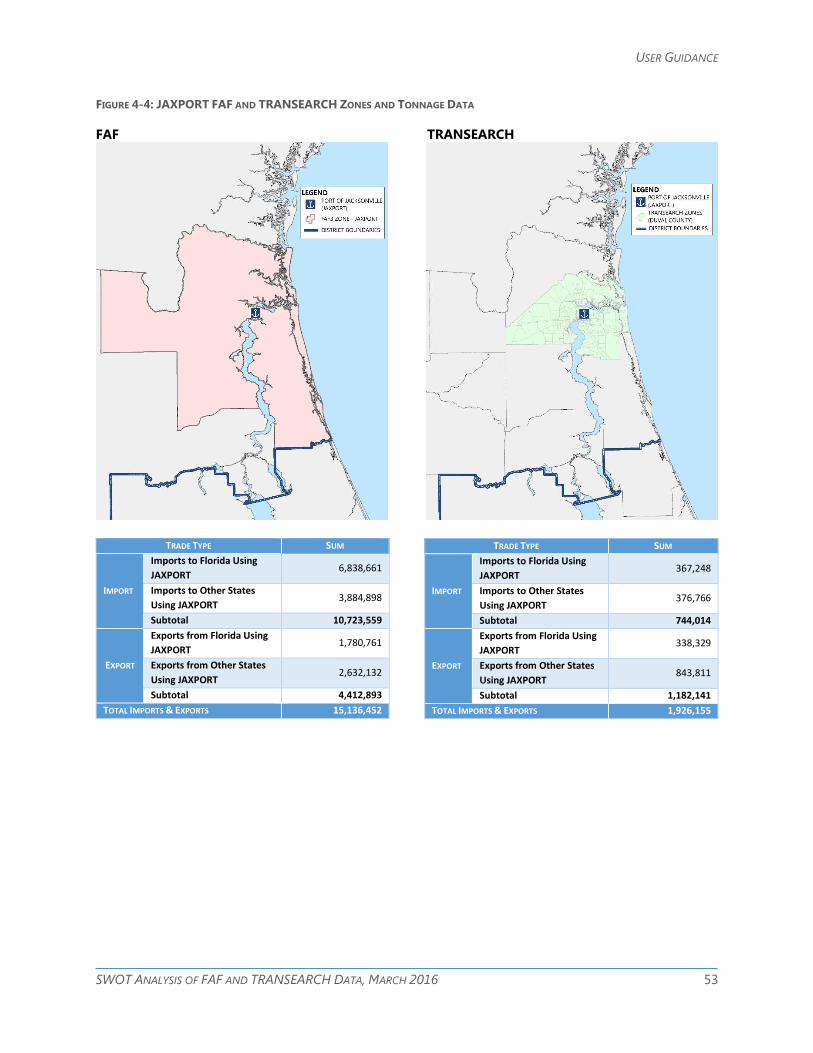
USER GUIDANCE
SWOT ANALYSIS OF FAF AND TRANSEARCH DATA, MARCH 2016 53
FIGURE 4-4: JAXPORT FAF AND TRANSEARCH ZONES AND TONNAGE DATA
FAF TRANSEARCH
TRADE TYPE SUM
IMPORT
Imports to Florida Using
JAXPORT 6,838,661
Imports to Other States
Using JAXPORT 3,884,898
Subtotal 10,723,559
EXPORT
Exports from Florida Using
JAXPORT 1,780,761
Exports from Other States
Using JAXPORT 2,632,132
Subtotal 4,412,893
TOTAL IMPORTS & EXPORTS 15,136,452
TRADE TYPE SUM
IMPORT
Imports to Florida Using
JAXPORT 367,248
Imports to Other States
Using JAXPORT 376,766
Subtotal 744,014
EXPORT
Exports from Florida Using
JAXPORT 338,329
Exports from Other States
Using JAXPORT 843,811
Subtotal 1,182,141
TOTAL IMPORTS & EXPORTS 1,926,155
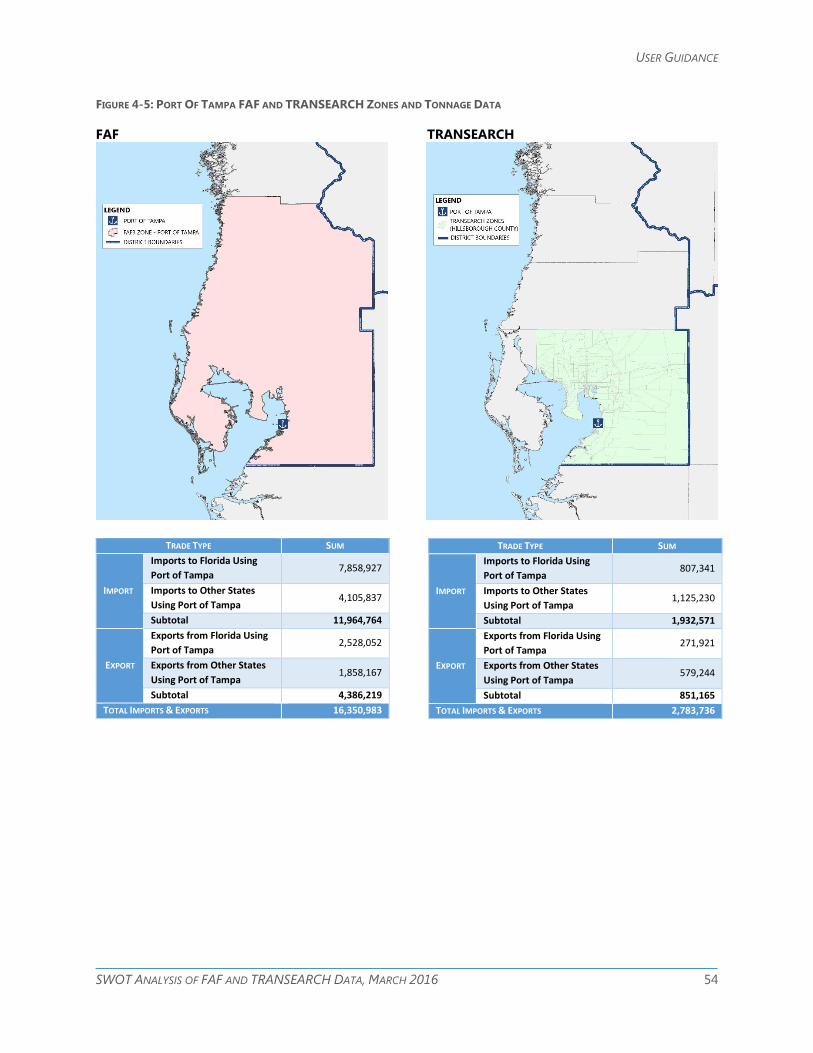
USER GUIDANCE
SWOT ANALYSIS OF FAF AND TRANSEARCH DATA, MARCH 2016 54
FIGURE 4-5: PORT OF TAMPA FAF AND TRANSEARCH ZONES AND TONNAGE DATA
FAF TRANSEARCH
TRADE TYPE SUM
IMPORT
Imports to Florida Using
Port of Tampa 7,858,927
Imports to Other States
Using Port of Tampa 4,105,837
Subtotal 11,964,764
EXPORT
Exports from Florida Using
Port of Tampa 2,528,052
Exports from Other States
Using Port of Tampa 1,858,167
Subtotal 4,386,219
TOTAL IMPORTS & EXPORTS 16,350,983
TRADE TYPE SUM
IMPORT
Imports to Florida Using
Port of Tampa 807,341
Imports to Other States
Using Port of Tampa 1,125,230
Subtotal 1,932,571
EXPORT
Exports from Florida Using
Port of Tampa 271,921
Exports from Other States
Using Port of Tampa 579,244
Subtotal 851,165
TOTAL IMPORTS & EXPORTS 2,783,736
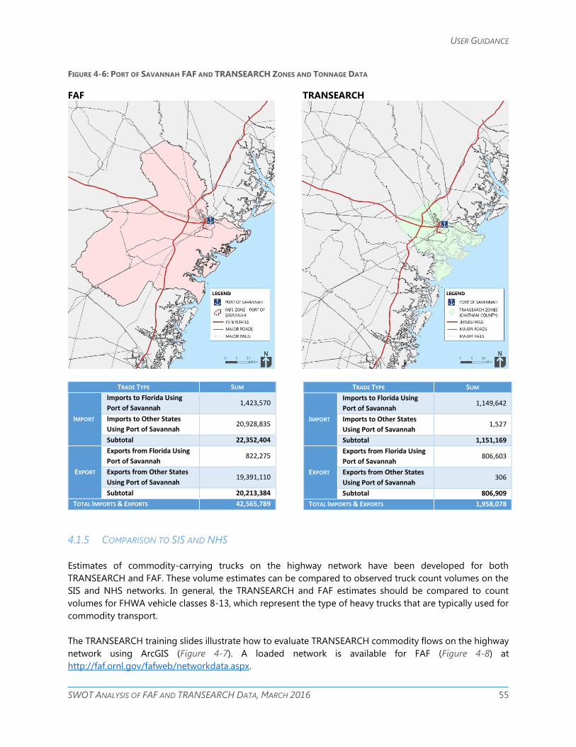
USER GUIDANCE
SWOT ANALYSIS OF FAF AND TRANSEARCH DATA, MARCH 2016 55
FIGURE 4-6: PORT OF SAVANNAH FAF AND TRANSEARCH ZONES AND TONNAGE DATA
FAF TRANSEARCH
TRADE TYPE SUM
IMPORT
Imports to Florida Using
Port of Savannah 1,423,570
Imports to Other States
Using Port of Savannah 20,928,835
Subtotal 22,352,404
EXPORT
Exports from Florida Using
Port of Savannah 822,275
Exports from Other States
Using Port of Savannah 19,391,110
Subtotal 20,213,384
TOTAL IMPORTS & EXPORTS 42,565,789
4.1.5 COMPARISON TO SIS AND NHS
Estimates of commodity-carrying trucks on the highway network have been developed for both
TRANSEARCH and FAF. These volume estimates can be compared to observed truck count volumes on the
SIS and NHS networks. In general, the TRANSEARCH and FAF estimates should be compared to count
volumes for FHWA vehicle classes 8-13, which represent the type of heavy trucks that are typically used for
commodity transport.
The TRANSEARCH training slides illustrate how to evaluate TRANSEARCH commodity flows on the highway
network using ArcGIS (Figure 4-7). A loaded network is available for FAF (Figure 4-8) at
http://faf.ornl.gov/fafweb/networkdata.aspx.
TRADE TYPE SUM
IMPORT
Imports to Florida Using
Port of Savannah 1,149,642
Imports to Other States
Using Port of Savannah 1,527
Subtotal 1,151,169
EXPORT
Exports from Florida Using
Port of Savannah 806,603
Exports from Other States
Using Port of Savannah 306
Subtotal 806,909
TOTAL IMPORTS & EXPORTS 1,958,078
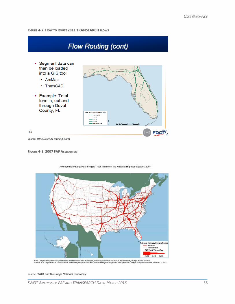
USER GUIDANCE
SWOT ANALYSIS OF FAF AND TRANSEARCH DATA, MARCH 2016 56
FIGURE 4-7: HOW TO ROUTE 2011 TRANSEARCH FLOWS
Source: TRANSEARCH training slides
FIGURE 4-8: 2007 FAF ASSIGNMENT
Source: FHWA and Oak Ridge National Laboratory
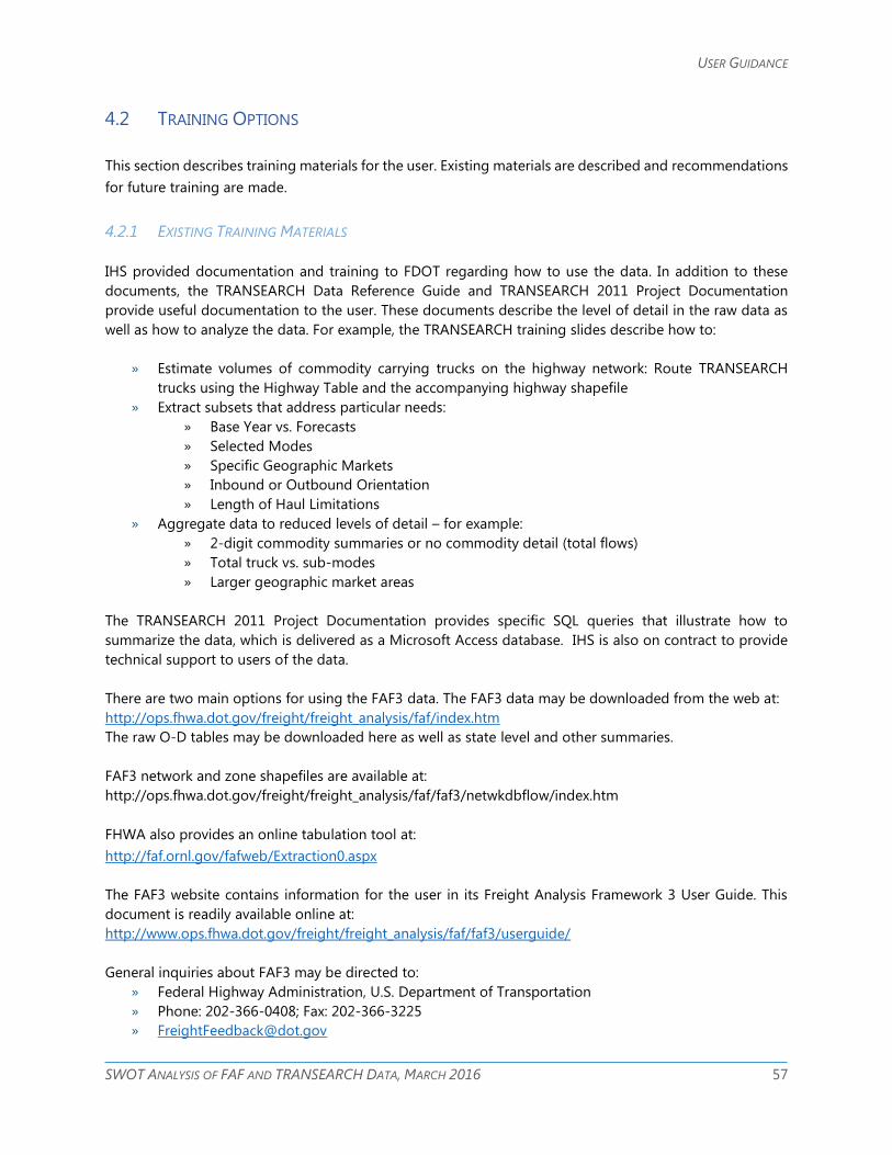
USER GUIDANCE
SWOT ANALYSIS OF FAF AND TRANSEARCH DATA, MARCH 2016 57
4.2 TRAINING OPTIONS
This section describes training materials for the user. Existing materials are described and recommendations
for future training are made.
4.2.1 EXISTING TRAINING MATERIALS
IHS provided documentation and training to FDOT regarding how to use the data. In addition to these
documents, the TRANSEARCH Data Reference Guide and TRANSEARCH 2011 Project Documentation
provide useful documentation to the user. These documents describe the level of detail in the raw data as
well as how to analyze the data. For example, the TRANSEARCH training slides describe how to:
» Estimate volumes of commodity carrying trucks on the highway network: Route TRANSEARCH
trucks using the Highway Table and the accompanying highway shapefile
» Extract subsets that address particular needs:
» Base Year vs. Forecasts
» Selected Modes
» Specific Geographic Markets
» Inbound or Outbound Orientation
» Length of Haul Limitations
» Aggregate data to reduced levels of detail – for example:
» 2-digit commodity summaries or no commodity detail (total flows)
» Total truck vs. sub-modes
» Larger geographic market areas
The TRANSEARCH 2011 Project Documentation provides specific SQL queries that illustrate how to
summarize the data, which is delivered as a Microsoft Access database. IHS is also on contract to provide
technical support to users of the data.
There are two main options for using the FAF3 data. The FAF3 data may be downloaded from the web at:
http://ops.fhwa.dot.gov/freight/freight_analysis/faf/index.htm
The raw O-D tables may be downloaded here as well as state level and other summaries.
FAF3 network and zone shapefiles are available at:
http://ops.fhwa.dot.gov/freight/freight_analysis/faf/faf3/netwkdbflow/index.htm
FHWA also provides an online tabulation tool at:
http://faf.ornl.gov/fafweb/Extraction0.aspx
The FAF3 website contains information for the user in its Freight Analysis Framework 3 User Guide. This
document is readily available online at:
http://www.ops.fhwa.dot.gov/freight/freight_analysis/faf/faf3/userguide/
General inquiries about FAF3 may be directed to:
» Federal Highway Administration, U.S. Department of Transportation
» Phone: 202-366-0408; Fax: 202-366-3225
USER GUIDANCE
SWOT ANALYSIS OF FAF AND TRANSEARCH DATA, MARCH 2016 58
FHWA has provided numerous webinars and listening sessions on how to use the FAF data for analysis.
These are found at the http://ops.fhwa.dot.gov/freight/freight_analysis/faf/index.htm site. These include:
» “Using FAF Data for Freight Planning”
» “How the FAF Can Help You”
» “Using Freight Analysis Framework Data in Economic Analysis”
» “Using Freight Analysis Framework Data for Freight Planning”
» Archived FAF Listening Sessions from December 2013 and January 2014 provide additional material
on the FAF data products
Finally, in addition to the main data development report, documentation on the network assignment and
how it was prepared can be found in the FAF3 FREIGHT TRAFFIC ANALYSIS: Final Draft Report by Batelle.
The report was submitted to Oak Ridge National Laboratory on March 23, 2001 and can be accessed
through the following link: http://faf.ornl.gov/fafweb/Data/Freight_Traffic_Analysis/faf_fta.pdf.
4.2.2 TRAINING RECOMMENDATIONS
While the existing training materials are already prepared, are readily accessible, and are fairly
comprehensive, the following adjustments are recommended to better facilitate user understanding.
While the existing TRANSEARCH training and documentation materials provide valuable information on the
assembly and usage of the data, the casual user may feel overwhelmed by the amount of information that
is presented. Additionally, the training slides contain a limited number of example applications. The training
slides focus more on “what the dataset is” than “what the dataset can do” in application. A condensed
version of the background with an expanded examples section may provide more practical information to
new or occasional analysts. Ideally, the examples will show step-by-step how the analysis can be conducted
using readily available processing tools such as Microsoft Access and ESRI ArcGIS.
In addition, improved naming conventions would help users understand the current TRANSEARCH
documentation. In the version that was received by our consultant team, the TRANSEARCH data was
accompanied by a total of seven documentation files. The naming of these files is rather unclear, as “Project
Documentation” can be easily confused with “Methodology Documentation” or “Reference Guide”. FDOT
(or IHS) may rename these before distribution to enhance their usefulness. Possible improved names are:
» “TRANSEARCH Field Descriptions and Querying Processes” instead of “TRANSEARCH 2011 Project
Documentation”
» “TRANSEARCH Dataset Construction” instead of “TRANSEARCH Methodology Documentation”
» “TRANSEARCH Field Codes and Geographies” instead of “TS Reference Guide”
Reorganizing the content would also help the user. Field descriptions and field codes, which are currently
in two separate documents, would logically fit into one document along with the description of
TRANSEARCH geographies. The Querying Processes illustrations fit logically into the training guide.
The FAF online tabulation tool makes the FAF product very easy to use. The documentation, also online, is
straightforward and it coherently describes the data limitations. However, it is difficult to determine based
on the documentation how the FAF differs from TRANSEARCH or whether FAF can be used for fairly specific
flow questions such as those related to port flows. Therefore, while the existing documentation is good and
useful, a few enhancements can make it more practical to the end user.
USER GUIDANCE
SWOT ANALYSIS OF FAF AND TRANSEARCH DATA, MARCH 2016 59
The following recommendations are made for commodity flow training modules.
4.2.2.1 Overview of Data and Analysis Purposes
The data should be briefly described and key terms like “commodity flow” and “modes” defined. Analysis
purposes can be contrived based on actual examples from the FMTP, regional freight plans, and other
documents. Illustrations should be utilized where possible.
4.2.2.2 Data Construction and Data Limitations
The user should be briefly acquainted with the basics of the underlying data (e.g., the CFS and BMI models).
A single table can be used to list each data source used in the data development. The practical emphasis
should be twofold. First, the training should demonstrate that the data were developed for user applications,
and that developing flow estimates from these underlying data sources is a big part of that. Second, it
should convey the uncertainties that are inherent in the data and help users understand the implications of
these limitations on analysis and interpretation of findings.
4.2.2.3 Application Examples
The training should first define various types of analysis. For example, different processes are used to
analyze flows by mode vs. production tonnages. The training should enumerate all of the common types of
analysis and provide a step-by-step overview on how to analyze each type. Next, examples in each category
should be demonstrated. Hands-on examples in Microsoft and ESRI platforms will show the user the details
of conducting analysis. The demonstration should inform the user on how to produce (or analyze) the
information as well as how to interpret the findings. Discussion of data limitations is an integral part of the
interpretation of findings.
4.3 DATA PURCHASE CONSIDERATIONS
The TRANSEARCH data provides Florida with the opportunity to evaluate commodity flows at a very detailed
level. IHS offers a variety of purchase options, including:
» Geographic level of detail: available levels include the state, county, zip code or TAZ levels
» Commodity level of detail: STCC4 is often used, but more or less detail may be an option (depending
on the commodity)
» Commodity coverage: the company will prepare estimates of commodities that are not typically
covered for clients that are interested
» Scenario offerings: while this category has many options, commonly requested scenarios are
typically based around macroeconomic scenarios. For example, the State of Florida purchase
includes high-medium-low flow estimates based on optimistic and pessimistic socioeconomic
conditions.
Full consideration of potential uses can help FDOT assess whether to purchase TRANSEARCH data and at
what level of customization. Each purchase option has its pros and cons. The more detailed data can be
used to answer more detailed questions as described throughout this report. For questions regarding very
specific industries, commodities, or geographic areas, TRANSEARCH will likely provide the best insights.
USER GUIDANCE
SWOT ANALYSIS OF FAF AND TRANSEARCH DATA, MARCH 2016 60
Alternately, experienced analysts may be able to develop a commodity flows with a similar level of detail
using readily available sources. For example, the user can disaggregate FAF data based on Census or
Infogroup employment data combined with production/consumption information from various sources.
The user could also try to replicate the IHS process of constructing commodity flow data based on county
level information in an economic modeling construct. Depending on the geography and commodity
coverage of the analysis, the amount of information can quickly become overwhelming to manage.
However, for a high level of detail or a broad analysis area, this option may be viable.

USER GUIDANCE
SWOT ANALYSIS OF FAF AND TRANSEARCH DATA, MARCH 2016 61
INTENTIONALLY LEFT BLANK
SWOT ANALYSIS OF FAF AND TRANSEARCH DATA, MARCH 2016 62
APPENDIX A
COMMODITY CLASSES USED IN FAF AND
TRANSEARCH

COMMODITY CLASSES USED IN FAF AND TRANSEARCH
SWOT ANALYSIS OF FAF AND TRANSEARCH DATA, MARCH 2016 63
INTENTIONALLY LEFT BLANK
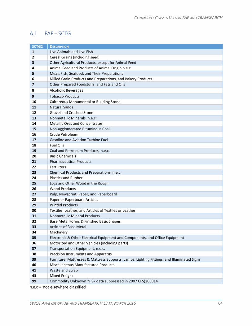
COMMODITY CLASSES USED IN FAF AND TRANSEARCH
SWOT ANALYSIS OF FAF AND TRANSEARCH DATA, MARCH 2016 64
A.1 FAF – SCTG
SCTG2 DESCRIPTION
1 Live Animals and Live Fish
2 Cereal Grains (including seed)
3 Other Agricultural Products, except for Animal Feed
4 Animal Feed and Products of Animal Origin n.e.c.
5 Meat, Fish, Seafood, and Their Preparations
6 Milled Grain Products and Preparations, and Bakery Products
7 Other Prepared Foodstuffs, and Fats and Oils
8 Alcoholic Beverages
9 Tobacco Products
10 Calcareous Monumental or Building Stone
11 Natural Sands
12 Gravel and Crushed Stone
13 Nonmetallic Minerals, n.e.c.
14 Metallic Ores and Concentrates
15 Non-agglomerated Bituminous Coal
16 Crude Petroleum
17 Gasoline and Aviation Turbine Fuel
18 Fuel Oils
19 Coal and Petroleum Products, n.e.c.
20 Basic Chemicals
21 Pharmaceutical Products
22 Fertilizers
23 Chemical Products and Preparations, n.e.c.
24 Plastics and Rubber
25 Logs and Other Wood in the Rough
26 Wood Products
27 Pulp, Newsprint, Paper, and Paperboard
28 Paper or Paperboard Articles
29 Printed Products
30 Textiles, Leather, and Articles of Textiles or Leather
31 Nonmetallic Mineral Products
32 Base Metal Forms & Finished Basic Shapes
33 Articles of Base Metal
34 Machinery
35 Electronic & Other Electrical Equipment and Components, and Office Equipment
36 Motorized and Other Vehicles (including parts)
37 Transportation Equipment, n.e.c.
38 Precision Instruments and Apparatus
39 Furniture, Mattresses & Mattress Supports, Lamps, Lighting Fittings, and Illuminated Signs
40 Miscellaneous Manufactured Products
41 Waste and Scrap
43 Mixed Freight
99 Commodity Unknown *( S= data suppressed in 2007 CFS)205014
n.e.c = not elsewhere classified

COMMODITY CLASSES USED IN FAF AND TRANSEARCH
SWOT ANALYSIS OF FAF AND TRANSEARCH DATA, MARCH 2016 65
A.2 TRANSEARCH – 2-DIGIT STCC CODES
STCC2 DESCRIPTION
100 Farm Products
800 Forest Products
900 Fresh Fish or Marine Products
1000 Metallic Ores
1100 Coal
1300 Crude Petrol. or Natural Gas
1400 Nonmetallic Minerals
1900 Ordnance or Accessories
2000 Food or Kindred Products
2100 Tobacco Products
2200 Textile Mill Products
2300 Apparel or Related Products
2400 Lumber or Wood Products
2500 Furniture or Fixtures
2600 Pulp, Paper or Allied Products
2700 Printed Matter
2800 Chemicals or Allied Products
2900 Petroleum or Coal Products
3000 Rubber or Miscellaneous Plastics Products
3100 Leather or Leather Products
3200 Clay, Concrete, Glass or Stone
3300 Primary Metal Products
3400 Fabricated Metal Products
3500 Machinery
3600 Electrical Equipment
3700 Transportation Equipment
3800 Instruments, Photographic Goods, Optical Goods, Watches, or Clocks
3900 Miscellaneous Products of Manufacturing
4000 Waste or Scrap Materials
4100 Miscellaneous Freight Shipments
4200 Containers, Carriers or Devices, Shipping, Returned Empty
4300 Mail or Contract Traffic
4400 Freight Forwarder Traffic
4500 Shipper Association Traffic
4600 Miscellaneous Mixed Shipments
4700 Small Packaged Freight Shipments
4900 Hazardous Materials
5000 Secondary Traffic
6000 Unclassified
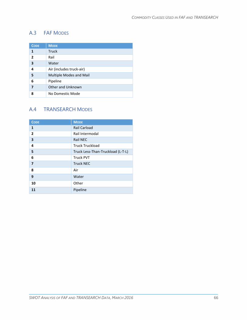
COMMODITY CLASSES USED IN FAF AND TRANSEARCH
SWOT ANALYSIS OF FAF AND TRANSEARCH DATA, MARCH 2016 66
A.3 FAF MODES
CODE MODE
1 Truck
2 Rail
3 Water
4 Air (includes truck-air)
5 Multiple Modes and Mail
6 Pipeline
7 Other and Unknown
8 No Domestic Mode
A.4 TRANSEARCH MODES
CODE MODE
1 Rail Carload
2 Rail Intermodal
3 Rail NEC
4 Truck Truckload
5 Truck Less-Than-Truckload (L-T-L)
6 Truck PVT
7 Truck NEC
8 Air
9 Water
10 Other
11 Pipeline

COMMODITY CLASSES USED IN FAF AND TRANSEARCH
SWOT ANALYSIS OF FAF AND TRANSEARCH DATA, MARCH 2016 67
INTENTIONALLY LEFT BLANK