TRANSACTIONS OF SOCIETY OF ACTUARIES 1984 VOL. 36 … · 2011-11-03 · The following paper is intended to acquaint actuaries with a simple and, we hope, practical application of

TRANSACTIONS OF SOCIETY OF ACTUARIES 1984 VOL. 36

P R A C T I C A L A P P L I C A T I O N S O F T H E R U I N F U N C T I O N

GEORGE E. RECKIN, DANIEL J. SCHWARK,* AND JOHN B. SNYDER II

A B S T R A C T

The following paper is intended to acquaint actuaries with a simple and, we hope, practical application of the ruin function technique in the determination of the C-2 mortality risk reserve needed for individual life insurance business. The goal is not the introduction of any new mathematical theory, as this field has been admirably explored by the more capable hands acknowledged herein. Rather, the paper seeks to provide working actuaries with a readable nontechnical introduction to this subject.

The paper gives a qualitative explanation of the theoretical basis of the ruin function technique. Several variations of the theory are discussed and then applied to an actual life insurance company situation. The results of each method are compared. Some of the limitations of the ruin function approach are pointed out. Finally, a mathematical appendix is presented to allow the reader to apply these techniques without having to consult outside references.

In the final analysis, the reader should realize that contingency surplus quantification is in its infancy in most life insurance companies. Therefore, the application of methods to determine the appropriate surplus level is as much an art as it is a science. That is, in spite of the high-powered mathematical theory underlying risk analysis, the results must be scru- tinized under the light of reason and experience.

I. B A C K G R O U N D

At some point in almost every life actuary 's career, he will be asked to examine an insurance company's current retention limit or evaluate its contingency surplus requirements. Three commonly posed questions along these lines are the following:

1. How much contingency surplus is realistically needed to cover the risk of random mortality fluctuations?

* Mr. Schwark, not a member of the Society, is an actuarial assistant with Milliman and Robertson, Inc.

453

454 PRACTICAL APPLICATIONS OF THE RUIN FUNCTION

2. How much addit ional risk is entailed when an insurance company increases its retent ion limit by a given amount?

3. How much surplus should be made available to cover random claim variations if a new line of bus iness is to be in t roduced?

These questions can be approached in several different ways. Histor- ically, many insurance companies have related retention limits and surplus requirements using industry-wide practices or "rule of thumb" techniques. An example of this would be setting a company's retention limit equal to 1 percent of its total capital and surplus.

Recently, however, actuaries have turned to statistical means to quantify variations in mortality experience. One of the first approaches was to use the distribution branch of collective risk theory. This generally involved examining one year's claims and establishing "confidence limits" as upper bounds of claims variation.

An alternative to the distribution branch Of collective risk theory is the ruin function. Ruin theory holds the advantage over distribution theory of looking at ruin continuously rather than at discrete points. Based on some of the texts listed in the bibliography, the four basic techniques used in evaluating ruin functions are (1) the convolution method, (2) the Monte Carlo method, (3) the Laplace transform inversion method, and (4) the method of moments. The first two methods lend themselves to numerical solutions but generally require advanced computer hardware and are expensive to use. The third method, involving the Laplace transform, offers few analytical solutions but some hope in using numerical means. The last approach, the method of moments, is easy to apply and inexpensive but is restricted by the accuracy and detail of the underlying data.

Using a variation of the method of moments suggested by Mr. Newton L. Bowers [13] and Mr. John A. Beekman [8], one can inexpensively produce reasonable results over finite or infinite time frames using only limited data.

Ultimately, the actuary must take the results of whichever method he chooses and employ his best judgment as to their reasonableness. Such judgment must include a basic understanding of the principles underlying the method used, knowledge of current industry practices, and reflection of state insurance department desires.

11. MATHEMATICAL BASIS OF THE RUIN FUNCTION

The formulation of the ruin function as described in Mr. Beekman's paper "A Ruin Function Approximation" [8] is briefly summarized: Un- derlying all the ruin theory work used in formulating this paper is a distribution function, P(z), which is the probability that, given that a claim

PRACTICAL APPLICATIONS OF THE RUIN FUNCTION 455

has occurred, its amount will be less than or equal to amount z. From a practical standpoint, it is the estimation of this function that takes the most time and incurs the greatest expense in the practical application of the method. A detailed breakdown of claims and in-force data by age and face amount, as required in the ideal application, is generally laborious and expensive to derive.

Also defined is another function, N(t), which is the random number of claims occurring in time period t. However, time t is generally defined in terms of operational time or the time for a claim to occur or N(t) = t. That is, if a life insurance company were to have 50 claims in a calendar year, then t = 50 would represent one calendar year from an operational time point of view. Generally, N(t) is assumed to have a Poisson distribution as discussed in Mr. Paul M. Kahn's "An Introduction to Collective Risk Theory and Its Application to Stop-Loss Reinsurance" [19].

Based on these definitions, a value p, can be found that is the first moment (or mean) of P(z). That is, p, is the average amount of a claim, given that a claim has occurred. Therefore, the quanti typ,t can be thought of as an aggregate net premium over time t.

If claims never deviated from the mean, a premium equal to the net premium would cover claims, and there would be no need for concern about financial ruin due to adverse claims experience. However, this is not the case in the real world. Therefore, in addition to the net premium, a company must protect itself from ruin due to adverse fluctuations in claims experience by starting with an initial risk reserve (initial contingency surplus), usually denoted by u, and collecting an amount in addition to the net risk premium. The amount paid in addition to the net premium is called a security loading and is really part of the gross premium profit margin that the policyholder pays. That is, the gross premium, besides covering expenses and benefits, inherently provides for periodic contri- butions to a risk reserve to offset adverse experience. The security loading is often represented by h; and ht represents the aggregate security loading collected through time t.

An additional item to be defined is the random variable X;, which represents projected claim amounts. Therefore, each random variable X, has as its distribution P(z), and E727 Xi represents the aggregate claims paid up to time t.

Thus, the company's current risk reserve U(t) at time t, which is a measure of the likelihood of ruin, can be symbolically stated by

N(t)

u(t) = . + (p, + x ) t - ~x~. i = 1

4 5 6 PRACTICAL APPLICATIONS OF THE RUIN FUNCTION

Since U(t) is useful as a measure of potential ruin (ruin occurring when U(t) < 0), the ruin function is the probability that U(t) will become less than zero within a time period t. The key is to try to quantify those elements that affect U(t) so as to minimize the probability of ruin within certain limits.

This is done by defining an additional random variable Z. Z is defined as the maximum excess of claims over income, examined continuously. Symbolically,

I N(t) 1 Z = maximum ~ X , - t(p, + X) . o,~t<~ Li~ I

Since it is the random variable Z that is to be quantified, Z must somehow be estimated. On the basis of the work of Mr. Beekman and Mr. Bowers, we assert that the incomplete gamma function is a good approximation to Z.

Several underlying assumptions of collective risk theory should be pointed out before proceeding. Generally, collective risk theory deals with an " o p e n " group having the attributes of (1) independence, (2) stationarity, and (3) exclusion of multiple events. The concept of an open group is comparable to a stationary population in which claimants are continually replaced. It is because of the open group assumption that the underlying mortality rate can be assumed to remain constant over time.

The assumption of independence is the basis for analyzing random mortality fluctuations. Independence implies that the occurrence of any one event is not influenced by nor does it influence the occurrence of any other events.

The concept of stationarity deals with the independence of the events with regard to commencement time. That is, the occurrence of events may be a function of the duration of a time period, but their occurrence should not be affected by the point at which the time measurement period starts.

The exclusion of multiple events is a simplifying assumption closely related to the independence of individual events and the choice of the Poisson distribution. It states that the probability of more than one claim occurring during an infinitesimal time interval is zero.

111. MODEL COMPANY

To determine the practical applicability of the ruin function to the contingency surplus problem, some actual insurance company in-force data are needed for a test case. Because the values that are of greatest interest

P R A C T I C A L A P P L I C A T I O N S OF T H E R U I N F U N C T I O N 457

to this analysis are extreme variations from the mean, the need for accurate data in testing is paramount.

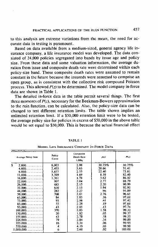
Based on data available from a medium-sized, general agency life insurance company, a life insurance model was developed. The data con- sisted of 24,000 policies segregated into bands by issue age and policy size. From these data and some valuation information, the average duration from issue and composite death rate were determined within each policy-size band. These composite death rates were assumed to remain constant in the future because the insureds were assumed to comprise an open group, as is consistent with the collective risk compound Poisson process. This allowed P(z) to be determined. The model company in-force data are shown in Table 1.

The detailed in-force data in the table permit several things. The first three moments of P(z), necessary for the Beekman-Bowers approximation to the ruin function, can be calculated. Also, the policy-size data can be changed to test different retention limits. The table shown implies an unlimited retention limit. If a $50,000 retention limit were to be tested, the average policy size for policies in excess of $50,000 in the above table would be set equal to $50,000. This is because the actual financial effect

T A B L E I

MODEL LIFE INSURANCE COMPANY IN-FORCE DATA

Composite [ Average Policy Size Policy Death Rate ' p(z) P(z)

Count [ 1.000q

$ 2,000 . . . . . . . . . . . 4 , 0 0 0 . . . . . . . . . . .

6,000 . . . . . . . . . . . 11,000 . . . . . . . . . . . 16,000 . . . . . . . . . . . 22,000 . . . . . . . . . . . 26,000 . . . . . . . . . . . 33,000 . . . . . . . . . . . 44,000 . . . . . . . . . . . 50,000 . . . . . . . . . . . 63,000 . . . . . . . . . . . 73,000 . . . . . . . . . . . 83,000 . . . . . . . . . . . 93,000 . . . . . . . . . . .

I00,000 . . . . . . . . . . . 130,000 . . . . . . . . . . . 155,000 . . . . . . . . . . . 226,000 . . . . . . . . . . . 355,000 . . . . . . . . . . . 550,000 . . . . . . . . . . .

1,000,000 . . . . . . . . . . .

6,903 2,455 5,877 3,399 1,36 I

907 685

2.98 5.63 2.55 1.69 i .78 2.04 2.15

30 .75% 20.66 22.40

8.59 3.62 2.77 2.20

30 .75% 51.41 73.81 82.40 86.02 88.79 90.99

610 282 708

84 93 55 43

370 20 43 79 16 4 6

2.13 2.27 2.61 2.85 2.98 2.28 2.05 2.85 1.82 2.78 2.84 2.31 4.19

1.94 .96

2.76

1.58

2.60

92.93 93.89 96.65

.36 97.01

.41 97.42

.19 97.61 i

.13 i 97.74 [ 99.32

.05 99.37 • 18 99.55 .34 99.89 .06 99.95 .03 99.98 .02 100.00


on the life insurance company would be the same whether a claim was $50,000 or $500,000.

If the Beekman-Bowers approach is going to be used, either (1) data such as given in the table must be available, (2) the first three moments of the distribution of a claim, given that a claim occurs, must be known, or (3) the moments of P(z) must be derived by making assumptions as to the mathematical characteristics of the distribution.

IV. APPLICATION OF THE RUIN FUNCTION

Based on the extensive data from the model company, the necessary parameters to utilize the Beekman-Bowers approximation of the ruin function can be derived. The first analysis looks at an unlimited retention limit and an infinite operational time frame. Later in this paper, the results assuming a finite time period are discussed.

From the calculation of the first three moments of the distribution P(z), a grid is constructed that summarizes the various initial risk reserves or contingency surplus amounts needed at various probabilities of ruin and security loading percentages. A particular probability of ruin reflects the assigned probability of claims exceeding income plus the initial risk reserve. That is, a 1 percent level from the grid gives the required value of the initial risk reserve so that, along with the security loading assumption, the probability of ruin is one chance in 100. This can also be thought of as a confidence limit: with the risk reserve shown and the assumed security load, there is a 99 percent probability that ruin will not occur. Again, it should be emphasized that this is over an infinite time frame.

As mentioned previously, another important aspect of establishing a level of contingency surplus is estimating the level of security loading that is appropriate. The grid of initial risk reserve values looks at various confidence levels for various security loading assumptions. The security loading, h, is usually taken as a percentage of the mean claims, p,. Since this security loading is explicitly or implicitly built into the gross premium when a product is priced, the security loading appears to be intrinsically related to the pricing profit margins. Because the profit margin inherently contains loads for adverse fluctuations in all assumptions (interest, expenses, lapses, deaths, and so on), a good estimate of h for individual life insurance policies might be the ratio of the present value of statutory profits to the present value of premiums. That is, h might typically be about 5-10 percent of mean claims for many blocks of nonparticipating individual life insurance.

A summary of the resulting initial risk reserves for the unlimited retention, infinite time horizon situation is given in Table 2.

PRACTICAL APPLICATIONS OF THE RUIN FUNCTION

TABLE 2

R U I N F U N C T I O N A N A L Y S I S

M O D E L C O M P A N Y D A T A W I T H G A M M A D I S T R I B U T I O N

U N L I M I T E D R E T E N T I O N , I N F I N I T E T I M E P E R I O D

(Results in $1,000s)

459

SECURITY LOADING

AS A PERCENTAGE

OF MEAN CLAIMS

2 . . . . . . . . . . . . . . . . . . .

3 . . . . . . . . . . . . . . . . . . . 4 . . . . . . . . . . . . . . . . . . .

5 . . . . . . . . . . . . . . . . . . .

6 . . . . . . . . . . . . . . . . . . .

7 . . . . . . . . . . . . . . . . . . .

8 . . . . . . . . . . . . . . . . . . .

9 . . . . . . . . . . . . . . . . . . .

10 . . . . . . . . . . . . . . . . . .

15 . . . . . . . . . . . . . . . . . . 20 . . . . . . . . . . . . . . . . . . 30 . . . . . . . . . . . . . . . . . . 40 . . . . . . . . . . . . . . . . . . 5 0 . . . . . . . . . . . . . . . . . .

10%

$9,649 4,895 3,309 2,514 2,037 1,717 1,489 1,317 1,183 1,075

749 581 408 317 259

VALUE OF INITIAL RISK RESERVE WITH PROBABILITY OF RUIN:

5% I%

$19,540 10,034 6,862 5,275 4,321 3,684 3,228 2,885 2,618 2,403 1,755 1,426 1,086

909 797

.1%

$29,466 15,207 10,452 8,072 6,642 5,688 5,005 4,492 4,092 3,772 2,805 2,315 1,814 1,554 1,393

$12,620 6,436 4,372 3,339 2,718 2,303 2,005 1,782 1,608 1,468 1,044

827 603 485 410

.01%

$39,407 20,397 14,057 10,885 8,980 7,709 6,799 6,116 5,584 5,158 3,873 3,223 2,562" 2,222 2,012

One interesting sidelight of the infinite time period ruin function approach is that it is independent of the number of policies exposed to risk, unlike the methods used in distribution theory.

An analysis of several different retention levels under the infinite time period assumption reveals the effects of limiting the maximum risk re- tained by an insurance company. Tables 3 - 6 look at retention limits of $25,000, $50,000, $100,000, and $200,000. As might be expected, the initial risk reserves increase smoothly from the $25,000 retention and approach the unlimited retention level as an upper bound.

As can be seen from the tables, the values of the initial reserve amounts appear to be relatively smooth and monotonically changing according to changes in the security loading and the probabili ty of ruin. The results from the ruin function look plausible for several reasons:

1. For a given probability of ruin, the initial risk reserve declines smoothly as the security loading increases.

2. For a given level of security loading, the initial risk reserve increases as the probability of ruin decreases.

3. In the aggregate, the lowest initial risk reserves occur at the lowest retention level.

4. The risk reserves increase between grids as the retention limit increases with the unlimited retention limit being the upper bound.

TABLE 3

RUIN FUNCTION ANALYSIS

MODEL COMPANY DATA WITH GAMMA DISTRIBUTION $25,000 RETENTION, INFINITE TIME PE~OD


SECURITY LOADING

AS A PERCENTAGE

OF MEAN CLAIMS

2 . . . . . . . . . . . . . . . . . . .

3 . . . . . . . . . . . . . . . . . . .

4 . . . . . . . . . . . . . . . . . . .

5 . . . . . . . . . . . . . . . . . . .

6 . . . . . . . . . . . . . . . . . . .

7 . . . . . . . . . . . . . . . . . . .

8 . . . . . . . . . . . . . . . . . . .

9 . . . . . . . . . . . . . . . . . . .

10 . . . . . . . . . . . . . . . . . . 15 . . . . . . . . . . . . . . . . . . 20 . . . . . . . . . . . . . . . . . . 30 . . . . . . . . . . . . . . . . . . 40 . . . . . . . . . . . . . . . . . 50 . . . . . . . . . . . . . . . . . .


10% 5%

$1,734 $2,258 872 1,136 584 762 440 575 354 462 296 387 255 334 224 294 200 263 181 238 124 163 95 125 66 88 51 69 42 57

1%

$3,474 1,749 1,174

886 714 599 517 455 407 369 254 196 138 109 92

.1% .01%

$5,214 $6,954 2,626 3,504 1,764 2,353 1,332 1,778 1,074 1,433

901 1,203 778 1,039 685 916 613 820 556 743 383 513 297 398 210 282 167 225 141 190

TABLE 4



$50,000 RETENTION, INFINITE TIME PERIOD


SECURITY LOADING

AS A PERCENTAGE

OF MEAN CLAIMS

2 . . . . . . . . . . . . . . . . . .

3 . . . . . . . . . . . . . . . . . .

4 . . . . . . . . . . . . . . . . . .

5 . . . . . . . . . . . . . . . . . .

6 . . . . . . . . . . . . . . . . . . .

7 . . . . . . . . . . . . . . . . . . .

8. 9 . . . . . . . . . . . . . . . . . .

10 . . . . . . . . . . . . . . . . . 15 . . . . . . . . . . . . . . . . . 20 . . . . . . . . . . . . . . . . . 30 . . . . . . . . . . . . . . . . . 4 0 . . . . . . . . . . . . . . . . .

5 0

10%

$3,047 1,532 1,027

775 623 522 450 396 353 320 218 168 117 91 75


5%

$3,969 1,998 1,341 1,012

815 683 589 519

I %

$6,109 3,078 2,068 1,563 1,260 1,058

914 805 721 654 452 350 249 198 167

.1%

$9,170 4,625 3,110 2,352 1,897 1,594 1,378 1,215 1,089

988 685 533 381 304 258

464 420 289 223 156 123 103

.01%

$12,231 6,171 4,151 3,141 2,535 2,131 1,842 1,625 1,457 1,322

918 716 513 411 350

460

TABLE 5

RUIN FUNCTION ANALYSIS M O D E L C O M P A N Y DATA WITH GAMMA DISTRIBUTION



SECURITY LOADING

AS A PERCENTAGE

OF MEAN CLAIMS

I t ~ . . . . . . . . . . . . . . . . .

2 . . . . . . . . . . . . . . . . . . .

3 . . . . . . . . . . . . . . . . . . .

4 . . . . . . . . . . . . . . . . . . .

5 . . . . . . . . . . . . . . . " . . . .

6 . . . . . . . . . . . . . . . . . . .

7 . . . . . . . . . . . . . . . . . . .

8 . . . . . . . . . . . . . . . . . . .

9 . . . . . . . . . . . . . . . . . . . .

10 . . . . . . . . . . . . . . . . . . 15 . . . . . . . . . . . . . . . . . . 20 . . . . . . . . . . . . . . . . . . 30 . . . . . . . . . . . . . . . . . . 40 . . . . . . . . . . . . . . . . . . 5 0 . . . . . . . . . . . . . . . . . .

10%

$4,795 2,413 1,619 1,221

983 824 711 625 559 506 346 266 186 145 120


5% I %

$9,619 4,855 3,267 2,473 1,996 1,678 1,451 1,281 1,148 1,042

724 564 404 323 275

.1%

$14,445 7,299 4,916 3,725 3,010 2,534 2,193 1,938 1,739 1,580 1,103

864 624 504 431

$6,247 3,148 2,114 1,598 1,288 1,081

933 822 736 667 460 356 251 198 166

.01%

$19,272 9,743 6,567 4,978 4,025 3,390 2,936 2,596 2,331 2,119 1,483 1,164

845 685 589

TABLE 6

R U I N F U N C T I O N ANALYSIS M O D E L C O M P A N Y D A T A W I T H G A M M A D I S T R I B U T I O N



SECURITY LOADING

AS A PERCENTAGE

OF MEAN CLAIMS

2 . . . . . . . . . . . . . . . . . .

3 . . . . . . . . . . . . . . . . . .

4 . . . . . . . . . . . . . . . . . .

5 . . . . . . . . . . . . . . . . . .

6 . . . . . . . . . . . . . . . . . .

7 . . . . . . . . . . . . . . . . . .

8 . . . . . . . . . . . . . . . . . .

9 . . . . . . . . . . . . . . . . . .

10 . . . . . . . . . . . . . . . . . 15 . . . . . . . . . . . . . . . . . 20 . . . . . . . . . . . . . . . . . 30 . . . . . . . . . . . . . . . . . 40 . . . . . . . . . . . . . . . . . 50 . . . . . . . . . . . . . . . . .


I % .1%

$12,420 $18,661 6,283 9,455 4,237 6,386 3,214 4,852 2,600 3,931 2,190 3,317 1,898 2,878 1,678 2,549 1,507 2,293 1,370 2,088

960 1,472 754 1,164 546 854 441 698 377 603

10% 5%

$6,184 $8,060 3, I 15 4,068 2,092 2,737 1,580 2,07 I 1,273 1,671 1,068 1,405

922 1,215 812 1,072 726 96 I 658 87 I 452 604 348 469 243 334 190 265 157 222

~01%

$24,904 12,630 8,538 6,492 5,264 4,446 3,861 3,422 3,08 I 2,807 1,987 1,577 1,164

957 831

461


Although these general trends are logical, they do not lend credence to the ruin function as an accurate method of measuring the risk of ruin due to random claims. This can only be done by comparing the results to other statistical methods.

V. DISTRIBUTION THEORY

As was mentioned previously, another method of measuring the risk of adverse claims experience is to use the distribution branch of collective risk theory. Again, this method uses the same sort of in-force data as was used for calculating the parameters for the gamma distribution approximation to the ruin function. However, the distribution theory looks only at various levels of adverse claims experience for one year 's claims.

There are several methods for utilizing the distribution branch of risk theory for a problem such as this. One of the most recent methods is a compound Poisson method presented by Mr. Harry H. Panjer in his paper, "The Aggregate Claims Distribution and Stop-Loss Reinsurance" [20].

Table 7 summarizes the results from the model company using the Panjer method. Several things should be pointed out:

1. The method looks at one year's claims and calculates the extra reserve, an amount in excess of the mean claim amount, that should be established for various confidence limits. A 99 percent confidence limit indicates that there is one chance in 100 that the aggregate claims will exceed the confidence amount plus the mean claim amount.

2. The results using the Panjer method are dependent on the number of policies in force. This is unlike the infinite time horizon ruin function, which is independent of the policy count.

3. The results assume an unlimited retention limit. 4. The Panjer distribution theory does not examine the probability of ruin at each

point in time. It looks at claims and excess claims at discrete points in time rather than continuously. That is, under the distribution theory approach, the company may appear solvent even though points of insolvency exist between the discrete points in time examined.

5. If the confidence limits numbers from the table can be thought of as a risk reserve, the method ignores the infusion of additional surplus from the security loads built into gross premiums.

To be consistent with the previously given ruin function tables, the table heading is labeled "probability of ruin" rather than "confidence limit." Because the distribution theory is a function of the number of policies studied, Table 7 summarizes the results for various portfolio sizes.

Some important items can be pointed out from the table. First, the risk reserve increases when going from the 2,400 policy case to the 24,000


TABLE 7

D I S T R I B U T I O N T H E O R Y A N A L Y S I S

MODEL COMPANY DATA USING PANJER METHOD UNLIMITED RETENTXON, ONE YEAR'S CLAIMS


463

MEAN

CLAIM

AMOUNT

VALUE OF RISK RESERVE WITH PROBABILITY OF RUIN:* NUMBER OF

POLICIES 10% 5% I% .1% .01%

2,400 $ 80 $ 81 $ 136 $ 285 $ 962 $1,112 24,000 802 3,224 3,507 4,090 4,840 5,527 240,000 . . . . . . . . . 8,020 1,068 1,435 2,179 3, I 01 3,931

* The probability of ruin represents the probability that aggregate claims for the year will exceed the risk reserve given plus the mean claim amount.

policy case but declines in going from the 24,000 policy case to the 240,000 policy case. The principal reason for the increase in going from the 2,400 policy case to the 24,000 policy case is the tenfold increase in the mean claim amount. The principal reason for the decline in the risk reserve in going from the 24,000 policy case to the 240,000 policy case is that as the sample size increases to very large amounts, the confidence limits approach the mean claim amount. If the model had an infinitely large number of policies, then the risk reserve under this method would become zero as the probability of aggregate claims exceeding the mean claim amount becomes zero.

Second, the risk reserve amount does increase monotonically as the probability of ruin declines.

Third, a comparison of the results in Table 7 to the unlimited retent ion- infinite time period ruin function results presented in Table 2 indicates that, at a 1 percent probability of ruin, the risk reserve using the Panjer method for the 24,000 policy case compares to the risk reserve assuming a security loading of 5 - 6 percent. For the company of medium to large size, the infinite time period ruin function appears to produce reasonable results based on the Panjer method. However, the method appears to overstate the risk reserve for a small company.

V1. EXPONENTIAL FUNCTION

Thus far the use of the gamma distribution approximation to the ruin function has required as much in-force detail as the Panjer method. The principal advantages to the use of the ruin function over the Panjer method are (1) the ruin function examines insolvency continuously rather than


discretely, and (2) the ruin function can be viewed over an infinite time horizon versus looking at claims in one-year increments.

The next step with regard to an analysis of the applicability of the ruin function is tO determine if there are any simplifying assumptions that can be made. In particular, are there any general assumptions that can be made with regard to the shape of the distribution P(z) such that reasonable risk reserve results can be generated utilizing limited policy data such as found in the NAIC convention blank? If this were possible, then the questions with regard to surplus requirements and retention limits could be answered without requiring detailed policy data, the compiling of which is time-consuming and expensive. It should be emphasized that the gamma distribution is still assumed to be a reasonable approximation to the ruin function; the remaining goal is to find an easy way to estimate the first three moments of P(z).

One suggested simplifying assumption is that the function P(z), the probability density function of claim size, given that a claim has occurred, can be approximated by an exponential function. If a function fix) is exponential in form, it can be generalized by

f(x) = 13e-~.

A detailed analysis of this assumption is given in the mathematical appendix to this paper, but from a practical point of view it implies that what is needed for the ruin function analysis is the average policy size and a retention limit assumption.

Based on the exponential assumption and the model insurance company average policy size, initial risk reserve amounts were constructed comparable to the original gamma distribution results. Tables 8-12 use the exponential assumption in the gamma approximation to the ruin function over an infinite time horizon at several retention limits.

A comparison of the results using an exponential distribution/gamma method and the full model detail using the gamma method is both encouraging and discouraging. The discouraging part arises because the results appear to be incompatible under the higher retention limit scenarios. This indicates that the exponential assumption is inappropriate for the model company on an unlimited retention basis. The principal reason for this is that the exponential function does not give adequate weight to the very large policy sizes. The results may also imply that the exponential assumption is inappropriate for most standard insurance companies.

The encouraging part is that the results assuming a smaller retention limit are much more compatible. Obviously part of the reason is that the low retention limits remove much of the weight that would be applied to

TABLE 8

RUIN FUNCTION ANALYSIS EXPONENTIAL CLAIM AMOUNT DISTRIBUTION, GAMMA DISTRIBUTION

UNLIMITED RETENTION, INFINITE TIME PERIOD


SECURITY LOADING

AS A PERCENTAGE

OF MEAN CLAIMS

2 . . . . . . . . . . . . . . . . . . .

3 . . . . . . . . . . . . . . . . . . .

4 . . . . . . . . . . . . . . . . . . .

5 . . . . . . . . . . . . . . . . . . .

6 . . . . . . . . . . . . . . . . . . .

7 . . . . . . . . . . . . . . . . . . .

8 . . . . . . . . . . . . . . . . . . .

9 . . . . . . . . . . . . . . . . . . .

10 . . . . . . . . . . . . . . . . . . 15 . . . . . . . . . . . . . . . . . . 20 . . . . . . . . . . . . . . . . . . 30 . . . . . . . . . . . . . . : . . 40 . . . . . . . . . . . . . . . . . . 50 . . . . . . . . . . . . . . . . . .

VALUE OF INITIAL RISK RESERVE WITH PROBABILITY OF RUIN;

i% .1%

$5,573 $8,366 2,808 4,218 1,887 2,836 1,426 2,145 1,149 1,730

965 1,453 833 1,256 734 1,107 657 I 992 596 900 411 623 319 485 226 346 179 276 151 234

1o~ 5%

$2,781 $3,621 1,398 1,823

937 1,223 707 923 568 743 476 623 410 537 361 473 322 423 292 383 199 263 153 203 106 142 83 112 68 93

.01%

$11,159 5,629 3,785 2,863 2,310 i,942 !,678 1,481 1,327 1,204

835 65O 466 373 317

"FABLE 9




SECURITY LOADING

AS A PERCENTAGE

OF MEAN CLAIMS

2 . . . . . . . . . . . . . . . . . . .

3 . . . . . . . . . . . . . . . . . .

4 . . . . . . . . . . . . . . . . . .

5 . . . . . . . . . . . . . . . . . .

6 . . . . . . . . . . . . . . . . . .

7 . . . . . . . . . . . . . . . . . .

8 . . . . . . . . . . . . . . . . . .

9 . . . . . . . . . . . . . . . . . .

10 . . . . . . . . . . . . . . . . . 15 . . . . . . . . . . . . . . . . . 20 . . . . . . . . . . . . . . . . . 30 . . . . . . . . . . . . . . . . . 4 0 . . . . . . . . . . . . . . . . .

50 . . . . . . . . . . . . . . . . .

IO~

$1,954 982 657 495 398 333 287 252 225 203 138 106 73 57 47

VALUE OF INITIAL RISK RESERVE WITH PROBABILITY OF RUIN~

5% 1%

$3,912 1,967 1,319

995 800 671 578 509 455 411 282 217 152 119 99

.1%

$5,870 2,953 1,98o 1,494 1,2o2 1,008

$2,544 1,278

857 646 519 435 375 329 294 266 182 139 97 76 63

.o1%

$7,828 3,938 2,641 1,993 1,6o4 1,344

869 1,159 765 1,02o 683 912 619 826 424 566 327 436 229 307 18o i 242 151 I 203

4 6 5

TABLE 10




SECURITY LOADING

AS A PERCENTAGE

OF MEAN CLAIMS

2 . . . . . . . . . . . . . . . . . .

3 . . . . . . . . . . . . . . . . . .

4 . . . . . . . . . . . . . . . . . .

5 . . . . . . . . . . . . . . . . . .

6 . . . . . . . . . . . . . . . . . .

7 . . . . . . . . . . . . . . . . . .

8 . . . . . . . . . . . . . . . . . .

9 . . . . . . . . . . . . . . . . . .

10 . . . . . . . . . . . . . . . . . 15 . . . . . . . . . . . . . . . . . 20 . . . . . . . . . . . . . . . . . 30 . . . . . . . . . . . . . . . . . 40 . . . . . . . . . . . . . . . . . 50 . . . . . . . . . . . . . . . . .

IO%

$2,597 1,305

874 659 530 444 382 336 300 271 185 142 98 77 63


5% I%

$5,202 2,619 1,758 1,327 1,069

897 774 681 610 552 380 293 207 164 137

.1%

$7,808 3,933 2,641 1,995 1,608 1,349 1,165 1,026

919 833 574 445 315 250 211

$3,381 1,70 I 1,140

860 692 580 500 440 393 356 244 188 131 103 86

.o1%

$10,413 5,246 3,524 2,663 2,146 1,802 1,556 1,371 1,228 1,113

768 596 423 337 285

TABLE t 1




SECURITY LOADING

AS A PERCENTAGE

OF MEAN CLAIMS

I ° ~ . . . . . . . . . . . . . . . .

2 . . . . . . . . . . . . . . . . . .

3 . . . . . . . . . . . . . . . . . .

4 . . . . . . . . . . . . . . . . . .

5 . . . . . . . . . . . . . . . . . .

6 . . . . . . . . . . . . . . . . . .

7 . . . . . . . . . . . . . . . . . .

8 . . . . . . . . . . . . . . . . . .

9 . . . . . . . . . . . . . . . . . .

10 . . . . . . . . . . . . . . . . . 15 . . . . . . . . . . . . . . . . . 20 . . . . . . . . . . . . . . . . . 30 . . . . . . . . . . . . . . . . . 40 . . . . . . . . . . . . . . . . . 50 . . . . . . . . . . . . . . . . .

10%

$2,775 1,395

935 705 567 475 409 360 322 291 199 152 106 82 68


5% 1%

$5,562 2,802 1,882 1,422 1,146

962 831 732 656 594 410 318 225 179 151

.1%

$8,349 4,209 2,829 2,140 1.726 1,450 1,252 1,105

989 897 621 483 344 275 233

$3,614 1,819 1,220

921 742 622 536 472 422 382 262 2O2 142 I11 93

.01%

$11,114 5,616 3,777 2,857 2,305 1,937 1,674 1,477 1,323 ! ,201

832 648 464 371 316

466


TABLE 12


E X P O N E N T I A L C L A I M A M O U N T D I S T R I B U T I O N , G A M M A D I S T R I B U T I O N

$ 2 0 0 , 0 0 0 R E T E N T I O N , I N F I N I T E T I M E P E R I O D


467

SECURITY LOADING [ VALUE OF INITIAL RISK RESERVE WITH PROBABILITY OF RUIN: !

AS A PERCENTAGE OF MEAN CLAIMS 10~b 5°~ I% . ]~o .0I~b

2 . . . . . . . . . . . . . . . . . .

3 . . . . . . . . . . . . . . . . . .

4 . . . . . . . . . . . . . . . . . .

5 . . . . . . . . . . . . . . . . . .

6 . . . . . . . . . . . . . . . . . .

7 . . . . . . . . . . . . . . . . . .

8 . . . . . . . . . . . . . . . . . .

9 . . . . . . . . . . . . . . . . . . 10 . . . . . . . . . . . . . . . . . 15 . . . . . . . . . . . . . . . . . 20 . . . . . . . . . . . . . . . . . 30 . . . . . . . . . . . . . . . . . 40 . . . . . . . . . . . . . . . . . 5 0 . . . . . . . . . . . . . . . . .

$2,781 $3,621 1,398 1,823

937 1,223 707 923 568 743 476 623 410 537 361 473 322 423 292 383 199 263 153 203 106 142 83 112 68 93

$5,573 $8,366 2,808 4,218 1,886 2,836 1,426 2,145 1,149 1,730

965 1,453 833 1.256 734 1,107 657 992 596 900 411 623 319 485 226 346 179 276 151 234

$11,159 5,629 3,785 2,863 2,310 1,942 1,678 1,48 I 1,327 1,204

835 650 466 373 317

the relatively few larger amount policies. If the retention limit being tested is relatively small ($25,000-$50,000) or the nature of the company's business is to issue smaller policies (less than $100,000), the exponential assumption may be reasonable and only data found in the annual statement are required.

Further, if the actuary did not have the facility for a detailed in-force analysis or felt such an analysis would not warrant the expense, he might elect the exponential assumption realizing the results would not be as accurate as a more detailed model.

VII. F I N I T E TIME RUIN FUNCTION ANALYSIS

Thus far, approximations to the ruin function have been viewed only over an infinite time horizon. An actuary might think that this is too conservative. Therefore, the question remains, can reasonable results be generated using some finite time period? The reader should be reminded that the time period is expressed in operational time, not in calendar time. A conversion from operational time to calendar time can be made by dividing the total operational units to be studied by the expected operational units in one calendar year. The expected operational units in one year is the expected number of claims in a year.


An approach to this question was suggested by Mr. Beekman and Mr. Bowers in their paper, "An Approximation to the Finite Time Ruin Func- tion" [l l, 12]. The results of using the Beekman-Bowers approximations for finite time intervals are summarized in Tables 13-16. The approximation was applied assuming an unlimited retention limit for calendar- year periods of one, five, ten, and twenty years.

Some anomalies occur that raise doubts concerning the reasonableness of the approximation, particularly when viewed over a short time period or at high probabilities of ruin. One of the anomalies is that the initial risk reserve, assuming a particular probability of ruin, first decreases but later increases as the security loading is increased. More reasonable results appear for the ten- and twenty-calendar-year scenarios with probabilities of ruin of 1 percent or less.

The reader should be cautioned with regard to the results of this method because of the inconsistencies in the reserve amounts and the limits posed by the use of operational time. With regard to the limits of operational time, the reader should be aware of the differences in operational time by company size. That is, the larger the company, the more units of operational time in one calendar year. The greater the number of units of operational time studied, the more the method approaches the infinite time situation and the more the results appear reasonable.

TABLE 13



U N L I M I T E D R E T E N T I O N , O N E C A L E N D A R Y E A R

(Results in $1.000s)

SECURITY LOADING I VALUE OF INITIAl. RISK RESERVE WITH PROBABILITY OF RUIN: I AS A PERCENTAGE I

OF MEAN CLAIMS 10~ 5% I% ' .1• .01%

2 . . . . . . . . . . . . . . . . . .

3 . . . . . . . . . . . . . . . . . .

4 . . . . . . . . . . . . . . . . . .

5 . . . . . . . . . . . . . . . . . .

6 . . . . . . . . . . . . . . . . . .

7 . . . . . . . . . . . . . . . . . .

8 . . . . . . . . . . . . . . . . . .

9 . . . . . . . . . . . . . . . . . .

10 . . . . . . . . . . . . . . . . . 15 . . . . . . . . . . . . . . . . . 2 0 . . . . . . . . . . . . . . . . .

3 0 . . . . . . . . . . . . . . . . .

4 0 . . . . . . . . . . . . . . . . .

50 . . . . . . . . . . . . . . . . .

$403 264 183 151 143 146 154 165 177 188 233 255 259 242 219

$561 497 422 386 375 377 386 398 409 420 453 459 435 399 363

$ 943 1,180 1,212 1.211 1.206 1,200 I, 194 1,186 1.177 1.166 1,099 1.029

906 813 743

$1,512 2,326 2,624 2,729 2,745 2,718 2,669 2,610 2,546 2,482 2,187 1,959 1,653 1,464 1,336

$2,092 3,564 4,184 4,422 4.466 4,412 4,311 4,188 4,057 3,927 3,361 2,952 2,439 2,145 1,959

TABLE 14



U N L I M I T E D R E T E N T I O N , F I V E C A L E N D A R Y E A R S


SECURITY LOADING AS A PERCENTAGE OF MEAN CLAIMS

2 . . . . . . . . . . . . . . . . . . 3 . . . . . . . . . . . . . . . . . . 4 . . . . . . . . . . . . . . . . . . 5 . . . . . . . . . . . . . . . . . .

6 . . . . . . . . . . . . . . . . . . 7 . . . . . . . . . . . . . . . . . . 8 . . . . . . . . . . . . . . . . . . 9 . . . . . . . . . . . . . . . . . . 10 . . . . . . . . . . . . . . . . . 15 . . . . . . . . . . . . . . . . . 20 . . . . . . . . . . . . . . . . . 30 . . . . . . . . . . . . . . . . . 40 . . . . . . . . . . . . . . . . . 50 . . . . . . . . . . . . . . . . .

10%

$51 I 316 355 437 513 573 616 643 657 603 619 539 404 317 259

V A L U E OF I N I T I A L RISK RESERVE W I T H PROBABILITY OF R U I N :

5% I%

$2,682 2,702

• 2,673 2,618 2,536 2,439 2,335 2,232 2,131 2,035 1,649 1,390 1,082

908 797

.1%

$5,506 6,177 5,946 5,541 5,122 4,736 4,39 I 4,086 3,819 3,583 2,763 2,299 1,811 1,554 1,393

$1,044 833 876 956

1,018 1,055 1,072 1,072 1,062 1,044

914 784 599 485 410

. 0 1 %

$ 8,589 10,067 9,590 8,752 7,93 I 7,206 6,583 6,051 5,596 5,205 3,913 3,233 2,561 2,222 2,012

TABLE 15



U N L I M I T E D R E T E N T I O N , T E N C A L E N D A R Y E A R S


SECURITY LOADING AS A PERCENTAGE OF MEAN CI_AIMS

2 . . . . . . . . . . . . . . . . . .

3 . . . . . . . . . . . . . . . . . .

4 . . . . . . . . . . . . . . . . . .

5 . . . . . . . . . . . . . . . . . . .

6 . . . . . . . . . . . . . . . . . . .

7 . . . . . . . . . . . . . . . . . . .

8 . . . . . . . . . . . . . . . . . . .

9 . . . . . . . . . . . . . . . . . .

I 0 . . . . . . . . . . . . . . . . .

15 . . . . . . . . . . . . . . . . . .

20 . . . . . . . . . . . . . . . . . . 30 . . . . . . . . . . . . . . . . . . 4 0 . . . . . . . . . . . . . . . . . . 5 0 . . . . . . . . . . . . . . . . . .

10%

$520 492 666 814 905 949 961 951 928 897 720 577 408 317 259

V A L U E OF I N I T I A l . RISK RESERVE W I T H PROBARII . ITY OF R U I N :

5% le/~,

$3.839 3,788 3,666 3,469 3,241 3,014 2,800 2,606 2,432 2,277 1,735 1,422 1.086

909 797

. l~r

$8.517 8,474 7.608 6,743 5,997 5,371 4,85 I 4,418 4.056 3,754 2,80 I 2,314 1,814 1,554 1.393

$ 1.268 1,228 1,395 1,498 1,531 1,517 1,476 1,421 1,359 1,295 1,016

823 603 485 410

.01%

$13,719 13,692 I 1,919 10,269 8,926 7,852 6,99 I 6,297 5,733 5,272 3,890 3,225 2,562 2,222 2,012

469


TABLE 16


M O D E l . C O M P A N Y D A T A W I T H G A M M A D I S T R I B U T I O N

U N L I M I T E D R E T E N T I O N , T W E N T Y C A L E N D A R Y E A R S


SECURITY LOADING

AS A PERCENTAGE

OF MEAN CLAIMS

IO~ . . . . . . . . . . . . . . . .

2 . . . . . . . . . . . . . . . . . .

3 . . . . . . . . . . . . . . . . . . 4 . . . . . . . . . . . . . . . . . .

5 . . . . . . . . . . . . . . . . . .

6 . . . . . . . . . . . . . . . . . .

7 . . . . . . . . . . . . . . . . . .

8 . . . . . . . . . . . . . . . . . .

9 . . . . . . . . . . . . . . . . . .

I 0 . . . . . . . . . . . . . . . . .

15 . . . . . . . . . . . . . . . . .

20 . . . . . . . . . . . . . . . . . 30 . . . . . . . . . . . . . . . . . 40 . . . . . . . . . . . . . . . . . 50 . . . . . . . . . . . . . . . . .

VALUE OF INITIAL RISK RESERVE WITH PROI~ABILITY OF RUIN:

I% .1%

$5,404 $12,374 5,214 10,901 4,789 9,106 4,298 7,661 3,836 6,544 3,434 5,686 3,094 5,023 2,812 4,508 2,577 4,102 2,380 3,777 1,754 2,805 1,426 2,315 1,086 1,814

909 1,554 797 1,393

10% 5%

$ 628 $1,662 920 1,955

1,220 2,157 1,355 2,164 1,378 2,073 1,340 1,942 1,272 1,802 1,193 1,667 1, I 13 1,543 1,036 1,43 !

747 1,042 581 827 408 603 317 485 259 410

.01%

$20,181 17,134 13,728 11,202 9,361 8,007 6,999 6,239 5,655 5,197 3,874 3,223 2,562 2,222 2,012

One additional item from the Beekman-Bowers paper should be pointed out. The authors prove a theorem which places an upper limit on the value of the ruin function. Briefly put, if +(u, 7) is the: probability of ruin given initial reserve u and over finite operational time period T, then

+(u, 7)<p_~T,

where Pz is the second moment of P(z) and u > 0.

VIII. OT HE R CONSIDERATIONS

In addition to the matters discussed in earlier sections, there are several items that should be addressed.

First, the results ignore the reserves released by death. That is, the risk reserves shown in the tables are conservative because they do not reflect that part of the face amount paid at death arises from the release of the reserve underlying the policy. One possible approximation to this quantity might be derived by taking the ratio of the reserves released by death from page 6 of the annual statement to claims incurred before reinsurance from Exhibit 11. One minus this ratio times the risk reserve might be thought of as the net risk reserve.

Second, the effects of interest were ignored. A zero interest rate is a simplifying and conservative assumption.

P R A C T I C A L A P P L I C A T I O N S OF THE RUIN F U N C T I O N 4 7 1

Third, the savings in reinsurance premiums were neglected. If a company increases its retention limit, an allocation of surplus is required to reserve for adverse claims fluctuation with regard to the additional risk. However, the cost of the allocation of surplus should be reduced by the loading portion of the additional reinsurance premiums that it would have paid if it had not increased its retention limit.

In conclusion, the ruin function can be an effective tool for measuring contingency surplus and retention limit requirements, provided the actuary understands and appreciates the limitations of the methods employed.

MATHEMATICAL APPENDIX

APPROXIMATION OF THE RUIN FUNCTION BY USE OF THE INCOMPLETE GAMMA DISTRIBUTION

Probability of ruin ~(u)given an initial risk reserve of u and security loading of k = 0pl (0 = a percentage, P l = the expected amount of a claim, given that a claim occurs): I

°

where

F(o0 = The complete gamma function = l ; t~- 'e- 'd t ;

2p3 + P2 ,

p, = nth moment of the distribution of the amount of claim, given that a claim occurs.

The initial integral shown above can be calculated by the following procedure.

The integral is standardized to the following:

; t " 'e 'dt , x = u/f3.

This integral is solved by two methods, the choice depending on whether x is greater or less than o~ + 5. (This relationship was found to yield acceptable convergence for each method after some testing.)

i John A. B e e k m a n [8].


1. Series expansion (x < et + 5):

t ~ ' e - ' d t = e-.3 + a (a + 1) -t ct(ct + 1)(et + 2) . . . .

2. Continued fraction (x/> a + 5):

f~ Ix I l - a l 2 - a I ] t ~ - t e - ' d t = e - x x ~ 1 + x + l + x + . . . .

The fraction

1 l - e t 1 2 - e t 1 ]

x + 1+ x + 1+ x +

is calculated by the method of convergents and is equal to the kth con- vergent when P k / q ~ = p ~ - ~/Ch_, within a specified degree of tolerance. Let

d 2 . , = m - c t , d2m +, = m ;

po=0, qo = 1, Pl = 1, ql =x;

then the convergents are calculated recursively by the following formula for m = 1, 2, 3 . . . k :

P2 . , = P z . , - , + d2.d92,~- z;

q z . , = q z m - , + d2,,,q2.,- 2;

P Z m + I = x P 2 , . + d 2 m + IP2,,, - I ;

qz m +, = x q 2 . , + d2. , + I q z , , , - , .

To calculate u for a given value of 6(u), the following iterative formula was derived based on the initial formula using Newton 's method. The starting value of u was set equal to a l l which is the expected value of aggregate claims.

f 3 [ ( f ~ t " - ' e - t d t ) - ~(u,,)(l + 0)]F(ct) U,, U,, +

+ l x " - ' e - r

FINITE TIME RUIN FUNCTION (GAMMA METHOD)-'

This method approximates the function O(u, /3 (the probability of ruin within T units of operational time given an initial risk reserve of u). Note: operational time is the average interval between claims; thus, one year of real time would equal the expected number of claims in a year 's units of operational time.

z John A. Beekman and Newton L. Bowers [ l l ] .

PRACTICAL APPLICATIONS OF THE RUIN FUNCTION 4 7 3

The method proceeds to deve lop et, [3, and P(Zr = 0). Then

, ( u , T ) = [ 1 - P ( Z r = O ) ] . ~ d t .

The above formula is calculated by the method shown previously. It should be noted that when T = 0% O(u) = 0~(u, T) and et and [3 equal the ct and 13 defined in the initial formula , and I1 - P ( Z r = 0)] = p,/(p, + h).

The following shows the deve lopmen t o f et, [3, and P ( Z r = 0) for the finite time gamma method.

0 = Securi ty loading percen tage ;

p . = nth momen t o f the amount o f a claim given that a claim occurs ;

h =Op,;

A = 1 - e-8.~°;

B A ( p 2 - 2 k p , ) ,

a, = I/2[,4 + ~/(A 2 - 4B)];

et2 = V2[A - X/ (A 2 - 4B)];

p, - oqpJ2k C2- V(A~- 4B)'

C , = - C - P ~ - 2 2k'

C,=P3 + P~. 3h 2h 2'

p2-e t ,C3 C, = ~ / ( a 2 _ 4B) '

C . = - C , - C , ;

Bp212X - ctzp ,

C7 - (p, + h)X/(A 2 _ 4B)'

Pl C~- - C~; p l + k

E[Zr] = P2 + C,e-~,r + C2e-~:r; 2h

474 P R A C T I C A L A P P L I C A T I O N S OF T H E RUIN F U N C T I O N

E[Z~] = C, + C,e-",T + C,e-Q~r;

h P[Zr = O] = + C6e-"'T+ CTe-~2r;

p l + h

E[ZZr] E[Z,]

13 = E-[-~r]r] (1 - P [ Z r = O ] ) '

E[Zr] 0 t - -

13(1 - P [ Z , = 01)"

GAMMA M E T H O D - - - E X P O N E N T I A L DISTRIBUTION

The following formulas show the development of the first three moments of p, for use with the gamma method, based on an exponential distribution.

R = Retention limit; 1 (without regard to retention limit

13= (Average policy size) restrictions);

f ix ) = 13e -x~ (exponential distribution);

p,= ffx13e-~dx + f~R13e-~dx 1 e-nO

13 1 3 '

p2 = x 2 e-"~dx+ 2 e-~,~dx

2 2Re -Ra 2e-Ra

132 13 132 ,

P3= f~x313e-x~dx + f~R'13e-x~dx 6 3R2e - ~ 6Re -R~ 6e - ~

133 13 f~2 133

Exhibit 1 shows the function IGAM written in the APL language, which evaluates the incomplete gamma integral in the following form:

1 f ; p_te_,dt" F(oO

[ 1 ] [ 2 ] [ 3 ] [ 4 ] [ 5 ] [ 6 ] [ 7 ] [ B ] { 9 ] [ 1 0 ] [ 1 1 ] [ 1 2 ] [ 1 3 ] [ 1 4 ] [15] [16] [17] [18] [19] [20] [21] [22]

E X H I B I T I

v z 4 . a x o n M : . : ; a l _ ; t ~ l . 1 ; : : l ; p ; c ~ ; M ; ~ 2

A g ' V ~ t U ~ T E S T H E ~ # . # C O M P I _ E T E G ~ M b 4 ~ Z# .#TEGf i :AL ~ E T W E ~ ' # . ! :.C ~ H T , X [ . # r Z t 4 Z T ' v ' F ' O R ~ + ' 0 *

R • " . , '4-0r , ' . ' R D O E S H O T ~ L L O W ,'.,' ( 0 ,

- ) ( ; . , . . ) . .a+5) / l~ l~ R ~ L L O W S Ed~:aHCHII.JG TO *E~fi:* IF" X _ ) a ÷ 5 , elL 14- ~t .4-~

--'. 2~ .z 1 ~. 0 THE P O L L O W I H G LOOP C ~ L C U L ~ T E S THE I H T E ~ R ~ L ]~"r" SER:ZES E~.~P~HSZOIq,

L O O P 1 : Zlt-Zl +, 0 0 0 0 0 0 0 1 x L , 5 + J 0 0 0 0 0 0 0 0 K ( ( * - - " ) x ( : ' : R A L ) ÷ ~ L 1 ) - ~ ~ " 1 -',~- 1 - - Z l " + 0 x t Z 2 = Z l R ~RC~HCHES OUT OF LOOP I F " '2="- '1 TO ~ D E C I M A L F ' L A C E S , z 2 ~ - Z l

- )LOOP 1

I,~: ,* P~-O ~ W~- 1 04-1 ~ :,' R T H E P O L L O W ~ H G L O O P C A L C U L A T E S THE Z H T E G R A L ~ty COI. ITZFtUE~ F ~ : ~ C T Z O H S ,

LOOP 2 ; Z~--- 1 ~ Z 1 ~" * 0 0 0 0 0 0 0 1 X L , 5 + 1 0 0 0 0 0 0 0 0 X ( F' + a ) X ( , - ;< ) X ( ".c ~ ~ ) + ' A - 1 " ~ 0 X | = / Z 1 R ~ R ~ H C H E S OUT OF L O O P I F THE L ~ S T 2 COHVER:GEHTS ~ : E [ G U L L TO ~ [ , E C I M ~ L F ' L A C E S ,

P ( - I ~ p ~ + / ( H p : < ) x P ( . I ~ p ~ + / p X ( M - C t ) ~ 1

M4-M+ 1 ~ L O O P 2


The func t ion is dyadic with the left a rgument being the value of et and the right a rgumen t be ing the value o fx . The func t ion el iminates the need to use tables of the incomple te gamma densi ty funct ion and greatly reduces the effort required in apply ing the methodology out l ined in the paper.

REFERENCES

1. ABRAMOWITZ, M., and SEGUN, I., eds. Handbook o f Mathematical Func- tions. New York: Dover, 1968.

2. AMMETER, H. "The Calculation of Premium Rates for Excess of Loss and Stop Loss Reinsurance Treaties." In Nonproportional Reinsurance, edited by S. VAJDA. Brussels: Arithbel, 1955.

3. ANDERSEN, E. SPARgE. "On the Collective Theory of Risk in the Case of Contagion between the Claims," Transactions o f the Fifteenth International Congress o f Actuaries, New York, II (1957), 219-29.

4. BARTLETT, D. K., III. "Excess Ratio Distribution in Risk Theory," TSA, XVII (1965), 435-53.

5. BEARD, R. E., PENTIKAINEN, T., and PESONEN, E. Risk Theory. London: Methuen, 1969.

6. BEEKMAN, J. A. "Research on the Collective Risk Stochastic Process," Skan- dinavisk Aktuarietidskrift, XLIX (1966), 65-77.

7. . "Collective Risk Results," TSA, XX (1968), 182-99. 8. - - . "A Ruin Function Approximation," TSA, XXI (1969), 41-48. 9. . Author's review of discussions of "A Ruin Function Approximation,"

TSA, XX1 (1969), 277-79. 10. - - . Two Stochastic Processes. New York: Wiley, 1974. 11. BEEKMAN, J. A., and BOWERS, N. L. "An Approximation to the Finite Time

Ruin Function," Part I, Skandinavisk Aktuarietidskrift, LV (1972), 41-56. 12. ~ . "An Approximation to the Finite Time Ruin Function," Part 2, Skan-

dinavisk Aktuarietidskrift, LV (1972), 128-37. 13. BOWERS, N. L., JR. "Expansion of Probability Density Functions as a Sum

of Gamma Densities with Applications in Risk Theory," TSA, XVIII (1966), 125-37.

14. ~ . Discussion of "A Ruin Function Approximation," TSA, XXI (1969), 275-77.

15. - - . "An Upper Bound on the Stop-Loss Net Premium," TSA, XXI (1969), 211-17.

16. BOHLMANN, H. Mathematical Methods in Risk Theory. Berlin: Springer- Verlag, 1970.

17. FELLER, W. An Introduction to Probability Theory and Its Applications, Vol. I. 3d ed. New York: Wiley, 1968.

18. GRANDELL, J., and SEGERDAHL, C. O. "A Comparison of Some Approxi- mations of Ruin Probabilities," Skandinavisk AktuarietidJkrift, LIV (1971), 143-58.

PRACTICAL APPLICATIONS OF THE RUIN FUNCTION 477

19. KAHN, P. M. "An Introduction to Collective Risk Theory and Its Application to Stop-Loss Reinsurance," TSA, XIV (1962), 400-425.

20. PANJER, H. H. "The Aggregate Claims Distribution and Stop-Loss Reinsur- ance," TSA, XXXll (1980), 523-35.

21. PEARSON, K. Tables o f the Incomplete F-Function. Cambridge: University Press, 1965.

22. PHILIPSON, C. "A Review of the Collective Theory of Risk," Skandinavisk Aktuarietidskrift, LI (1968), 1-41.

23. SEAL, H. "Simulation of the Ruin Potential of Nonlife Insurance Companies," TSA, XXI (1969), 563-85.

24. - - . Stochastic Theory o f a Risk Business. New York: Wiley, 1969. 25. SEGERDAHL, C. O. "A Survey of Results in the Collective Theory of Risk."

In Probability and Statistics: The Harald Cramdr Volume, pp. 276-99. Upp- sala: Almqvist & Wikseli, 1959.

26. TAKACS, L. "On the Distribution.of the Supremum of Stochastic Processes with Interchangeable Increments," Transactions o f the American Mathe- matical Society, CXIX (1965), 367-79.

27. WOODDY, J. C. Study Note on Risk Theory. Chicago: Society of Actuaries, 1963.

DISCUSSION OF PRECEDING PAPER

J O H N A. B E E K M A N :

The authors of this paper have performed a great service by demonstrating uses of collective risk theory in the determination of the C-2 mortality risk reserve needed for individual life insurance business.

Since the publication of references [8], [9], [11], [12], and [14] of the paper, there have been a number of articles written which have discussed the accuracy of the gamma function approximate method for computing +(u). The following contains my observations on those papers in addition to the present one.

The results on E(Z) and Var(Z) derived in [7] were accurate, subject to the Poisson distribution for N(t), t>--O. It was acknowledged from the outset that the method was more accurate for O(u) than for ~(u, T). However, for a large portfolio, E{N(t)} could be 1,000 or so per year, justifying the use of the ~(u) technique. A key point is that some alternative techniques are so complicated that few practicing actuaries would use them. A very fine technique for approximating ~(u) developed by Olof Thorin and Nils Wiks- tad is introduced in [10], pages 74-76. However, to understand their method, the actuary should study the theory of functions of complex variables. One idea in the Thorin-Wikstad papers, which is helpful and can improve the accuracy of the gamma function methods, is to use a weighted sum of five exponential distributions, rather than a single exponential distribution, for P(z), the distribution of a single claim given that a claim has occurred. (See [10], 45, 46, 183, and 184.)

Another convolution type series for O(u) is in [7], but it seemed to have little utility. It now appears to offer potential for practical calculations. Some approximations to the series, including error analyses and examples, are presented in:

J. A. Beekman and C. P. Fuelling, "Risk Convolution Calculations," Scandinavian Actuarial Journal, 198 I, 151-64.

J. A. Beekman, "Risk Convolution Calculations II," pages 19-30 of Premium Calcu- lation in Insurance, F. deVylder et al. (eds.), D. Reidel Publishing, Dordrecht, Hol- land, 1984.

I am pleased that the authors applied the techniques of Harry Panjer to the same problem. Dr. Panjer's method is excellent and very helpful to the actuary. Section V of this paper is most valuable.

479

480 P R A C T I C A L A P P L I C A T I O N S O F T H E R U I N F U N C T I O N

The ruin function ideas can also be used in other settings. Dr. Clinton P. Fuelling and I used the same methods in modeling computer usage at our university. That paper ( " A Stochastic Model of Computer Use," C. P. Fuelling and J. A. Beekman, Scandinavian Actuarial Journal, 1980, 43- 52) also contained a simple algorithm for computing gamma distribution values. We join the authors in wanting to eliminate the need for using tables of the incomplete gamma density function.

Collective risk theory has been studied for many years and includes beau- tiful mathematical work by Professor Harald Cramrr and other researchers. (See [6].) But the ultimate test of the theory is whether it will be used. This excellent paper by Reckin, Schwark, and Snyder assures me that it will.

E L I A S S . W . SHIU:

In applying the method described in the paper, one should keep four points in mind. First, as pointed out in section VIII of the paper, the rate of interest is assumed to be zero in the model. However, in individual life insurance the interest rate is usually a much more dominant factor than the mortality rates. Second, it seems doubtful that the concept of an "open" group can be applied to individual life insurance. Indeed, H.L. Seal [11] concluded his note "The Poisson Process: Its Failure in Risk Theory" with the statement: "Poisson, renewal and Ammeter point processes have never been shown to occur in actuarial work." Third, the Beekman-Bowers approximation may not be sufficiently accurate. Seal ([10], p. 62) wrote that he would be reluctant to recommend its use. H.U. Gerber ([7], p. 128) suggested that "unless c~ = 1 and 13 = 1/R, the relative error of this approximation may become considerable if u is very large." (Here R denotes the adjustment coefficient, not the retention limit as in the paper.) Fourth, no limit is imposed on the growth of the risk reserve ([6], p. 10).

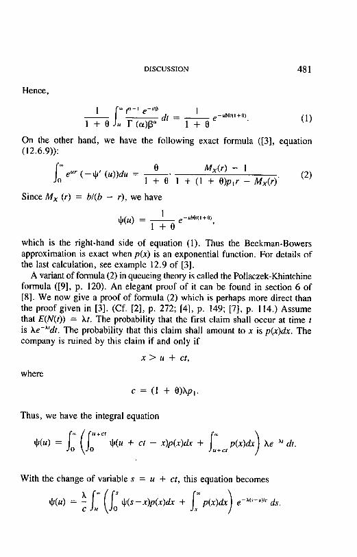
It should be pointed out that if the probability density function of claim size given that a claim has occurred, p(x), is exponential, the Beekman- Bowers approximation is exact ([1], p. 50). Let

p(x) = be -°x, x >- O.

It is easy to verify that

1 + 0 13-

b0

and

DISCUSSION 481

Hence,

1 r ~ t ~-I e -ar~ 1

1 + 0 J. F (o0~1 ~---------g d t - 1 +-----0 e-Ub°'O+°)" (1)

On the other hand, we have the following exact formula ([3], equation (12.6.9)):

f o 0 M x ( r ) - 1 e u r ( - ~ ' (u))du - 1 + 0 1 + (1 + O)plr - Mx(r)"

(2)

Since M x (r) = b/(b - r), we have

1 _ _ e-UbO#O +0)

tb(u)- I + 0

which is the right-hand side of equation (I). Thus the Beekman-Bowers approximation is exact when p(x) is an exponential function. For details of the last calculation, see example 12.9 of [3].

A variant of formula (2) in queueing theory is called the Pollaczek-Khintchine formula ([9], p. 120). An elegant proof of it can be found in section 6 of [8]. We now give a proof of formula (2) which is perhaps more direct than the proof given in [3]. (Cf. [2], p. 272; [4], p. 149; [7], p. 114.) Assume that E(N(t)) = ht. The probability that the first claim shall occur at time t is ke-X'dt. T h e probability that this claim shall amount to x is p(x)dx . The company is ruined by this claim if and only if

x > u + ct,

where

c = (1 + 0)Xp~.

Thus, we have the integral equation

So(r; s:+ @(u) = . @(u + ct - x )p (x )dx + ct p ( x ) d x ) he -x' dt.

With the change of variable s = u + ct, this equation becomes

s:(s; s: ) @(u) = _h @ ( s - x ) p ( x ) d x + p (x )dx e -x<"-">'< ds. c


Putting p = c/h and using the notation

So ( f . g)(z) = f(z-x)g(x)dx, z > O,

we have

p+(u) = e " p j ~ [ ( t ~ * p ) ( s ) + 1 - P(s)]e ,,Ods.

Differentiating, we obtain the integro-diffential equation

p+ ' (u) = +(u) - [(t~ * p)(u) + 1 - P(u)l. (3)

Let us multiply equation (3) by e r" and integrate with respect to u from 0 to 0o. Integrating by parts, we have

foer"t~(u)du= [ - O ( O ) + f o e r " ( - ~ ' ( u ) ) d u ] / r

and

Since

we obtain

~o e" (1 - P(u))du = [ - 1 + Mx(r)l/r.

~o Mx(r ) - 1 (4) eru(-~'(u))du = (1 - t~(O)) 1 - Mx(r ) + pr"

Hence formula (2) is proved if we can show that

4(0) = l/(1 + 0). (5)

To prove (5), consider equation (4) with r tending to zero. The left-hand side o f (4) converges to

- ~ o O'(u)du = ~(0) - ~(~)

= q,(o).

DISCUSSION 483

By L ' H 6 p i t a l ' s Rule, the r ight-hand side o f (4) converges to

Since

and

(1 - 0 ( 0 ) ) M'x (0)

-M'x (0) + p"

M ~ ( 0 ) = Pl

p = (1 + 0)p,,

formula (5) is proved. W e now give another proof of (5) which might be o f pedagogical interest

since we are treating the convolut ion as the mult ipl icat ion opera tor in a commuta t ive ring. Consider the convolut ion o f (3) with the constant function 1:

Since

p ~ ' * l = (~ - ~*p - 1 + P )* I

= +*1 - ~ * p * l - (1 - P ) * I .

Or, 1)(u) = f(x)dx

and P(0) = 0 by hypothesis ,

p(dg(u) - ~(0)) = (dg , 1)(u) - (~ * P)(u) - fo'

= (~ • (1 - p ) ) ( u ) - yo'

(1 - P(x))dx

(1 - P(x))dr. (6)

It can be shown that

l im (qJ * (1 - P))(u) = 0; u---~oo

thus

f ~ p(O - g,(o)) = o - J o

= - - P l .

(1 -- P(x))dx


Hence

t~(O) = pl/p

= l/(1 + 0)

as required. We note that exercise 11 in chapter 12 of [3] is an immediate consequence of equations (5) and (6).

In theory, formula (2) can be used to determine ~ for each given M x .

The appendix gives an integral representation for t~, but such contour inte- grals can be difficult to evaluate. However, ifp is a finite sum of exponential functions, we can derive an elegant expression for d~ as follows. By the method of partial fractions, we have

0 M x ( r ) - 1 = ~ C / r ( (7) 1 + 0 1 + (1 + O)plr - M x ( r ) i= I ri - r

(see section 12.6 of [3]). Thus, by formula (2)

~(U) = ~ Ci e-flu. (8) i=1

To find the coefficient Cj, multiply (7) by i) - r and let r tend to rj. Since

lim rj - r = - 1 r---~rj 1 + (1 + O)plr - M x ( r ) (1 + 0)p~ - M ' x (rj) '

we obtain

o r

0 M x ( r j ) - 1

1 + O ' M ' x (rj) - (1 + 0)p~ = Cjrj ,

Opl (9) Cj = M ' x (rj) - (1 + 0)pl

Formula (9) can be found on page 82 of [5], where it is derived by the residue theorem.

The following two relations can be useful for checking values. From equations (5) and (8) we immediately have

1 - ~ C i . I + 0 i~l

DISCUSSION 4 8 5

Multiply (7) by r; since lira Mx(r) = 0, we obtain /,----~ - - OO

0 -- ~ Ciri.

(1 + 0)2pl i=l

To conclude this discussion let me mention some references on ruin probabilities. Seal's book [10] is concerned with numerical probabilities of ruin in a finite time period for nonlife insurance companies. There are thirty- three pages of FORTRAN computer programs in its appendix. The book is supplemented by [12]. Thorin's paper [14] is a systematic review of his results on ruin probabilities. Its emphasis is on the calculation of the ruin probability for a finite time period by the Wiener-Hopf technique, under the assumption that the epochs of claims follow a renewal process.

APPENDIX

Denote the right-hand side of (2) by g(r). Since

o eru d?(u)du = [-t~(0) + g(r)]/r,

applying the complex inversion formula for the Laplace transformation ([13], chapter 7) gives

I f~,+i~ ~ ( u ) = ~-~ -,~

As

-d~(O) + g(r) e-r"dr, a<0 . (10)

lim g(r) = 1/(1 + 0) r---~0

= ~(0),

the point r = 0 is a removable singularity. Thus formula (10) can be sim- plified as

1 --Jc :+i= g(r) e -ru dr, 0 < c < R , ~J(U) = ~ -i~ 7

where R is the adjustment coefficient. This formula is equation (118) of [5].

R E F E R E N C E S

|. BEEKMAN, J.A. Two Stochastic Processes, New York: Wiley, 1974. 2. BORCH, K. The Mathematical Theory of Insurance, Lexington, Mass.: D. C. Heath,

1974.


3. BOWERS, N.L., GERBER, H.U., HICKMAN, J.C., JONES, D.A., AND NESBIq~F, C.J. Risk Theory, Part 5A Study Notes 52-1-82, Chicago: Society of Actuaries, 1982.

4. BOHLMANN, H. Mathematical Methods in Risk Theory, New York: Springer-Verlag, 1970.

5. CRAMI~R, H. "Collective Risk Theory," Skandia Jubilee Volume, Stockholm, 1955. 6. . "Historical Review of Filip Lundberg's Works on Risk Theory,"

Skandinavisk Aktuarietidskrift, LII (1969), Supplement, 6-12. 7. GERBER, H.U. An Introduction to Mathematical Risk Theory, Homewood, 111.:

Irwin, 1980. 8. LINDLEY, D.V. "The Theory of Queues with a Single Server," Proceedings, Cam-

bridge Philosophical Society, XLVIII (1952), 277-89. 9. SEAL, H.L. Stochastic Theory of a Risk Business, New York: Wiley, 1969.

10. . Survival Probabilities: The Goal of Risk Theory, New York: Wiley, 1978.

1 I. . "The Poisson Process: Its Failure in Risk Theory," Insurance: Math- ematics & Economics, I1 (1983), 287-88.

12. . "Numerical Probabilities of Ruin When Expected Claim Numbers Are Large," Mitteilungen der Vereinigung schweizerischer Versicherungsmathe- matiker, LXXXIII (1983), 89-103.

13. SPIEGEL, M.R. Schaum's Outline of Theory and Problems of Laplace Transforms, New York: Schaum, 1965; reprinted by McGraw-Hill.

14. THORIN, O. "Probabilities of Ruin," Scandinavian Actuarial Journal, 1982, 62- 102.

(AUTHORS' REVIEW DISCUSSION)

GEORGE E. RECK1N, DANIEL J. SCHWARK, AND JOHN B. SNYDER:

We wish to thank Professors Beekman and Shiu for the thought provoking comments outlined in their discussions.

Professor Beekman has pointed with encouragement to several alternative ruin probability evaluation methods. These methods would appear to hold considerable promise in areas of practical application. We would encourage all interested readers to investigate them more fully. It is unfortunate, however, that so much of the literature on this exciting subject is available only through foreign publications which are not often accessible to practicing actuaries.

Professor Shiu raises some fine points concerning the accuracy of the gamma approximation. We agree that ignoring interest in an infinite time ruin model is very conservative. In practice, however, we have found that the ruin technique still generates much higher feasible retention limits and lower risk reserve requirements than most insurance executives would com- fortably employ.

D~SCUSmON 487

We disagree with Professor Shiu's comments concerning the inaccuracy of the Poisson process in a real insurance company. In this regard, Professor Beekman was kind enough to supply some unpublished data developed by the late David Halmstad concerning the accuracy of the Poisson assumption in a large life insurance company. The results of this study verified the accuracy of the Poisson assumption using chi-square tests.

Professor Shiu also questions the accuracy of the Beekman-Bowers approximation. Although the accuracy of the method cannot be proven in a purely mathematical sense, except under some restricted assumptions, our experience with this and other risk theory techniques indicates that the method remains very useful as a guide to working actuaries. Practical work in this area is as much art and politics as science, and no method can be ascribed full credibility.

We hope that this paper and its discussion will encourage other actuaries to investigate and utilize the variety of statistical techniques that exist in this field.

Documents

TRANSACTIONS OF SOCIETY OF ACTUARIES 1984 VOL. 36 … · 2011-11-03 · The following paper is intended to acquaint actuaries with a simple and, we hope, practical application of