1

Trajic: An Effective Compression System forTrajectory Data

Aiden Nibali and Zhen He

Abstract—The need to store vast amounts of trajectory data becomes more problematic as GPS-based tracking devicesbecome increasingly prevalent. There are two commonly used approaches for compressing trajectory data. The first is the linegeneralisation approach which aims to fit the trajectory using a series of line segments. The second is to store the initial data pointand then store the remaining data points as a sequence of successive deltas. The line generalisation approach is only effectivewhen given a large error margin, and existing delta compression algorithms do not permit lossy compression. Consequently thereis an uncovered gap in which users expect a good compression ratio by giving away only a small error margin. This paper fills thisgap by extending the delta compression approach to allow users to trade a small maximum error margin for large improvementsto the compression ratio. In addition, alternative techniques are extensively studied for the following two key components of anydelta-based approach: predicting the value of the next data point and encoding leading zeros. We propose a new trajectorycompression system called Trajic based on the results of the study. Experimental results show that Trajic produces 1.5 timessmaller compressed data than a straight-forward delta compression algorithm for lossless compression and produces 9.4 timessmaller compressed data than a state-of-the-art line generalisation algorithm when using a small maximum error bound of 1meter.

Index Terms—Trajectory compression, spatial databases

F

1 INTRODUCTION

As GPS-based tracking devices become more popularmore trajectory data need to be stored. A trajec-tory comprises of a sequence of timestamped samplepoints, each containing a time, latitude and longitude.Using this representation a fleet of one thousand carseach recording a sample per second requires close to2 GB of storage space per day. Often a backlog ofsuch trajectory data need to be stored in a databases.Data compression algorithms can be applied to reducestorage requirements. Two contrasting state-of-the-artapproaches for compressing trajectory data are linegeneralisation and delta compression.

There are a large number of algorithms that take theline generalisation approach to compressing trajecto-ries [4], [11], [10], [15]. Line generalisation representsa trajectory using a series of linear segments createdby joining selected trajectory points. Compression isachieved by discarding unselected trajectory points.A maximum error threshold is enforced by ensuringthat the points discarded are within range of theline segments covering the points. The main problemwith this approach is that it can only achieve a goodcompression ratio when successive data points areclose to being linear. However, real-life trajectoriescan contain a lot of curvature and noise, sometimesaccompanied by low sampling rates which amplifythe negative effect of curves. The only way to improvecompression in these situations is for the user tospecify a large error margin (such as over 20 meters),but many users require higher precision.

Delta compression achieves lossless compression bystoring the difference between successive data points

• Aiden Nibali and Zhen He are with the Department of ComputerScience and Computer Engineering, La Trobe University, Bundoora,VIC, Australia.E-mail: dismaldenizen@gmail.com, z.he@latrobe.edu.au

in a trajectory rather than the points themselves. Sincethese deltas are typically small, they may be encodedto save space. In contrast to line generalisation, deltacompression is still able to achieve reasonable com-pression ratios despite any noise or curvature becauseit only requires successive points to be close to eachother rather than to lie within a straight line. Fur-thermore, line generalisation achieves no compressionfor a point that lies only a little outside the maxi-mum error bound, whereas delta compression is ableto smoothly degrade its compression ratio if pointsbecome further apart.

Figure 1 illustrates the tradeoff between compres-sion ratio and maximum error for line generalisation,delta compression, and line generalisation enhancedby delta compression. As we can see on the graph,delta compression (the single point labeled as Delta)has a zero error but a relatively poor compressionratio. In contrast line generalisation can achieve agood compression ratio but only after the maximumerror is relatively high. Even a combination of linegeneralisation and delta compression does not showany improvement in the compression ratio until themaximum error is relatively high. Therefore from thefigure we can see that there is currently an unfilledgap in which the user is willing to tolerate only asmall error in exchange for large improvements in thecompression ratio.

We have designed an algorithm called “Trajic”which can fill the above mentioned gap. Figure 1shows Trajic can achieve a good compression ratioin situations where the user is willing to give uponly a small amount of precision. In fact, even atzero error Trajic is able to achieve a relatively goodcompression ratio. Trajic has two core components: apredictor and a method for encoding residuals. Thepredictor guesses the value of the next data point andthen generates small residuals representing the dif-ference between the predicted and actual values. Theresidual encoding scheme attempts to use as few bits

2

Com

pre

ssio

n r

ati

o

Maximum error

good

poor

low high

Ideal

Delta Trajic

Line generalisation+ Delta

Line generalisation1

Figure 1. An abstract view of compression algorithmswith respect to a theoretical ideal (produced based onresults shown in Figure 15)

as possible to encode the number of leading zeros inthe residuals, and is able to achieve lossy compressionby discarding a number of least significant bits. Welimit the number of bits discarded to stay within themaximum user defined error margin.

Our Trajic compression algorithm is developed byextensively studying alternative algorithms for pre-dictors and leading zero encoding schemes. A com-parison was made between five different predictionalgorithms ranging from the simple “constant pre-dictor” (used in existing delta compression) to themore conceptually complicated cubic spline predictor.It was found that a simple and fast predictor, the“temporally-aware linear predictor”, results in themost accurate predictions. Hence Trajic utilises thispredictor.

We found different existing leading zero encodingschemes to be optimal for different actual residuallengths (the length of a residual without countingleading zeros). Furthermore, we discovered that inreal data sets residual lengths have a skewed distri-bution. This led to our novel method for encodingleading zeros which adapts to the distribution ofresidual lengths by incorporating a simple pre-passfrequency analysis step.

Finally, Trajic has linear run-time complexity (O(N))which is the same as simple delta compression. Incontrast line generalisation algorithms range in com-plexity from O(N log(N)) to O(N2).

Extensive experiments using real data sets showthat Trajic can produce 1.5 times smaller compresseddata than a straightforward delta compression algo-rithm (used in systems such as TrajStore [5]) for loss-less compression and 9.4 times smaller compresseddata than a state-of-the-art line generalisation algo-rithm when using a 1 meter error bound.

In summary, this paper makes the following threemain contributions.• We identify that neither of the existing methods

of line generalisation or delta compression, nora combination of the two, allow users to trade asmall amount of accuracy for large gains in thecompression ratio. This is a result of a systematicanalysis and experimentation of existing state-of-the-art line generalisation algorithms and existing

delta compression algorithms.• We develop the Trajic system to fill this important

gap in the existing literature. Within the Trajicsystem our main claim to novelty is the creationof a very effective and novel residual encodingscheme. A related contribution is making thedelta compression scheme span the spectrum be-tween lossless and lossy compression.

• We conduct extensive experiments demonstrat-ing the effectiveness of Trajic when applied toreal-world data sets. We systematically comparethe different algorithm across the three impor-tant metrics of compression/decompression time,compression ratio and error margin.

This paper begins by briefly discussing existing re-lated work and their shortcomings in Section 2.Section 3 describes the Trajic system, starting withthe predictor then continuing with the generationof residuals, leading zero encoding and finally themethod for storing residuals. Section 4 presents theexperimental results and finally Section 5 concludesthe paper.

2 RELATED WORKAs mentioned in the introduction there are two mainapproaches to compressing trajectories: line general-isation and delta compression. We will review theexisting work in both areas in addition to some othermethods that require knowledge of a road network.

2.1 Line generalisationOne of the most common trajectory compressionschemes is line generalisation [4], [11], [10], [6], [13],[21]. The line generalisation method originated fromcartographers wanting to use computers to extractfeatures from detailed data and represent them us-ing simple and readable maps. An important partof representing linear features is to solve the linegeneralisation problem.

The line generalisation problem can be de-fined as follows. Given an ordered set of n + 1points in the plane, V0, V1, ...Vn, let C, containingV0V1, ..., ViV i+ 1, ..., Vn−1Vn, be a chain with n linesegments. The problem is to find a modified C ′ con-taining less segments which approximates C withinan acceptable error margin, where the error marginis usually defined as the maximum perpendiculardistance from C ′ to C.

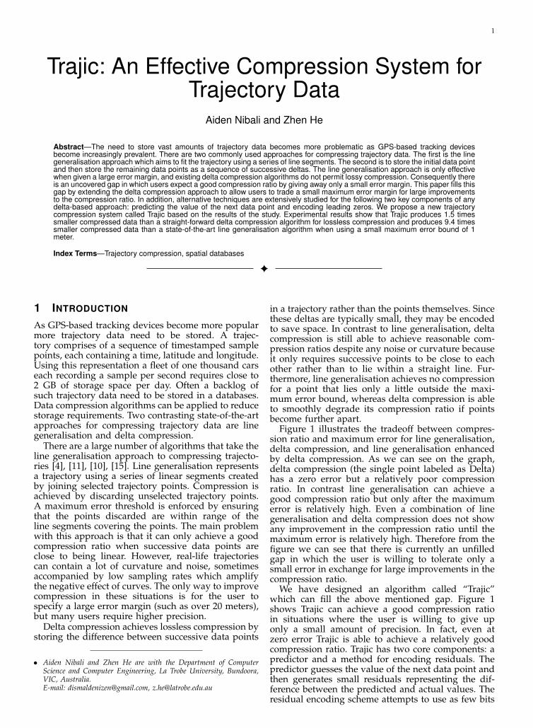
One of the most popular line generalisation algo-rithms is the top-down Douglas-Peucker (DP) algo-rithm [6], illustrated in Figure 2. At the beginning theentire set of points is approximated using a one linesegment connecting the first and last points of the set.Next the single long line segment is replaced by twoshorter line segments in which the end of the firstline segment and the start of the second line segmentcorrespond to the point that is the furthest (highestperpendicular distance) from the original single longline segment. This is recursively repeated until thereare no points whose maximum perpendicular distanceis higher than a user-defined threshold from the linesegment covering the point. The original DP algo-rithm has O(N2) time complexity, however, various

3

Selected point Unselected point

Max distance point

Max distance point

(a) After first line split (b) After second line split

Figure 2. Example illustrating the Douglas Peucker top-down line generalisation algorithm.

improvements have been proposed, including the oneby Hershberger et al. [8], which has a time complexityof O(N log(N)).

Another approach for solving the line generalisa-tion problem is the opening window approach [11].The opening window approach is an incrementalalgorithm that starts with a window that contains thefirst three points of the trajectory and then progres-sively “opens” the window until a single line segmentcan no longer represent all of the contained pointsaccurately enough. Once this happens, a single linesegment from the first point of the window to the sec-ond last point in the window is used to approximatethe current window and the second last point in thecurrent window becomes the start of the next window.This is repeated until the entire set of points have beenconnected by line segments. The opening windowalgorithm has O(N2) worst case time complexity.

When line generalisation methods are applied toachieve trajectory compression, the time dimensionmust be incorporated into the error metric. One wayof incorporating time is to use the synchronised eu-clidean distance (SED) [18]. SED measures the dis-tance from the original point to the approximatedpoint adjusted to the same timestamp. Another met-ric is the Meratnia-By time-distance ratio [11] wherespatial and temporal information are both used sepa-rately to decide whether a point is kept or discarded.For the temporal component, the ratio of the timetaken to travel the original versus approximated tra-jectory is used. For the spatial component, the positionof the original point is compared to its approximatedposition within the compressed trajectory.

The main limitation with the line generalisationapproach stems from the fact that it uses straight linesto approximate trajectories. Therefore, it works bestwhen trajectories are mostly linear. But in real lifethere are a lot of non-linear segments in trajectoriesdue to turning, noise and low sampling rates. Linegeneralisation requires very large error margins toachieve a good compression ratio in these scenarios.

2.2 Delta compressionThe standard simple delta compression algorithmstores a delta for each timestamp in the trajectory. Thedelta di for the ith timestamp equals pi - pi−1 where piand pi−1 are the trajectory point values at timestamp iand i−1 respectively. The above is typically performedseparately for each of the three components of time,longitude and latitude of the trajectory.

Existing literature in trajectory compression has al-most exclusively focused on line generalisation meth-ods, hence delta compression has been largely ig-nored in the past. However, the TrajStore [5] state-of-the-art trajectory database system only employs thestandard simple delta compression method definedabove. This simple method suffers from the followingthree shortcomings: it 1) employs a constant predic-tion policy; 2) uses a static leading zero encodingscheme; and 3) only performs lossless compression.The first shortcoming means TrajStore’s delta com-pression scheme essentially predicts the next datapoint to be exactly the same as the current pointand stores the difference as a delta. In contrast, thispaper explores a number of different prediction mod-els and conclude a temporally-aware linear predictorgives smaller deltas and hence better compressionratios. The second shortcoming of TrajStore’s deltacompression scheme is that it uses a static scheme toencode leading zeros. In contrast, this paper analyzesa number of different possible leading zero encod-ing schemes and concludes that our novel dynamicscheme gives the best performance. Finally, TrajStore’sdelta compression scheme only does lossless compres-sion. In contrast our Trajic performs both lossless andlossy compressing and hence can directly competeagainst the popular line generalisation methods whichare all lossy compression methods.

In addition to delta compression, TrajStore alsocompresses trajectories by clustering similar trajecto-ries together and storing only one representative tra-jectory per cluster. This is a complementary techniquethat may also be used in conjunction with our Trajicalgorithm.

2.3 Other methodsThere are other systems which use knowledge ofpredefined road networks and tracks to minimisethe space required when storing trajectories [3], [2].However, such systems are not very useful when thenetwork data is not available, or the moving objectsare not confined to well-defined tracks. The Trajiccompression scheme does not require such additionalnetwork information to compress trajectories.

Mahrsi et al. [7] proposed a one pass samplingbased method for trajectory compression which selec-tively decides if individual points should be discardedbased on whether the point can be predicted withina user defined error. They claim this method is morecomputationally efficient compared to the line gen-eralisation methods but at the same time allows an

4

PredictorResidual

Maker

Leading Zero

Encoder

Generator

ResidualPredicted pointTrajectory

Collect

Residuals

Entire

Residuals

Trajectory

Residuals

Approximate Point

Approximate points

Input: Original points

EncodedOutput:

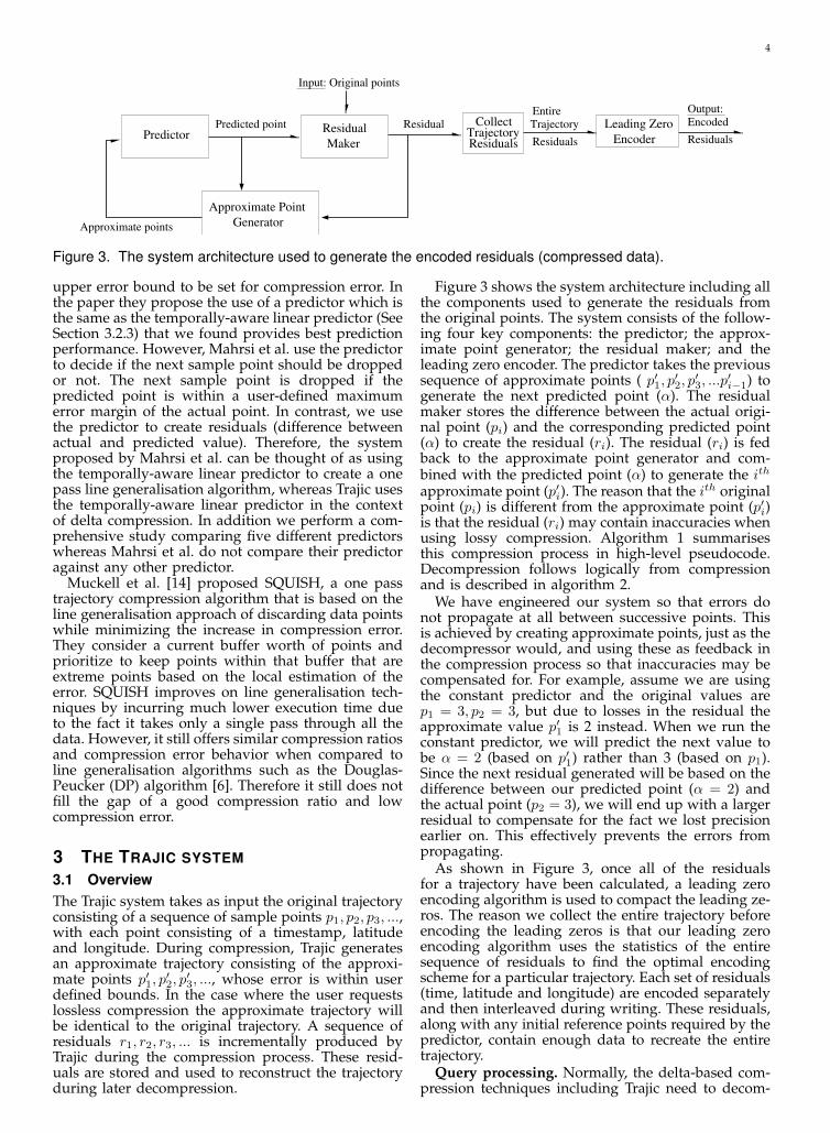
Figure 3. The system architecture used to generate the encoded residuals (compressed data).

upper error bound to be set for compression error. Inthe paper they propose the use of a predictor which isthe same as the temporally-aware linear predictor (SeeSection 3.2.3) that we found provides best predictionperformance. However, Mahrsi et al. use the predictorto decide if the next sample point should be droppedor not. The next sample point is dropped if thepredicted point is within a user-defined maximumerror margin of the actual point. In contrast, we usethe predictor to create residuals (difference betweenactual and predicted value). Therefore, the systemproposed by Mahrsi et al. can be thought of as usingthe temporally-aware linear predictor to create a onepass line generalisation algorithm, whereas Trajic usesthe temporally-aware linear predictor in the contextof delta compression. In addition we perform a com-prehensive study comparing five different predictorswhereas Mahrsi et al. do not compare their predictoragainst any other predictor.

Muckell et al. [14] proposed SQUISH, a one passtrajectory compression algorithm that is based on theline generalisation approach of discarding data pointswhile minimizing the increase in compression error.They consider a current buffer worth of points andprioritize to keep points within that buffer that areextreme points based on the local estimation of theerror. SQUISH improves on line generalisation tech-niques by incurring much lower execution time dueto the fact it takes only a single pass through all thedata. However, it still offers similar compression ratiosand compression error behavior when compared toline generalisation algorithms such as the Douglas-Peucker (DP) algorithm [6]. Therefore it still does notfill the gap of a good compression ratio and lowcompression error.

3 THE TRAJIC SYSTEM3.1 OverviewThe Trajic system takes as input the original trajectoryconsisting of a sequence of sample points p1, p2, p3, ...,with each point consisting of a timestamp, latitudeand longitude. During compression, Trajic generatesan approximate trajectory consisting of the approxi-mate points p′1, p

′2, p′3, ..., whose error is within user

defined bounds. In the case where the user requestslossless compression the approximate trajectory willbe identical to the original trajectory. A sequence ofresiduals r1, r2, r3, ... is incrementally produced byTrajic during the compression process. These resid-uals are stored and used to reconstruct the trajectoryduring later decompression.

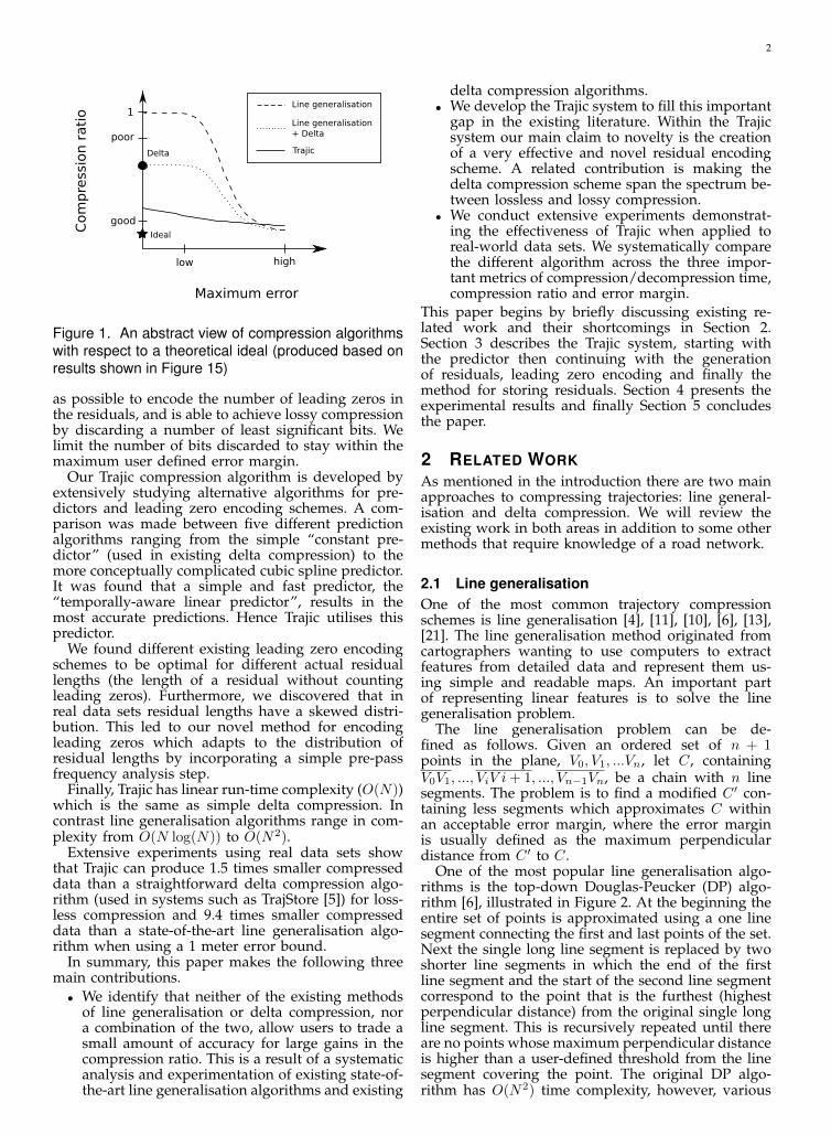
Figure 3 shows the system architecture including allthe components used to generate the residuals fromthe original points. The system consists of the follow-ing four key components: the predictor; the approx-imate point generator; the residual maker; and theleading zero encoder. The predictor takes the previoussequence of approximate points ( p′1, p′2, p′3, ...p′i−1) togenerate the next predicted point (α). The residualmaker stores the difference between the actual origi-nal point (pi) and the corresponding predicted point(α) to create the residual (ri). The residual (ri) is fedback to the approximate point generator and com-bined with the predicted point (α) to generate the ithapproximate point (p′i). The reason that the ith originalpoint (pi) is different from the approximate point (p′i)is that the residual (ri) may contain inaccuracies whenusing lossy compression. Algorithm 1 summarisesthis compression process in high-level pseudocode.Decompression follows logically from compressionand is described in algorithm 2.

We have engineered our system so that errors donot propagate at all between successive points. Thisis achieved by creating approximate points, just as thedecompressor would, and using these as feedback inthe compression process so that inaccuracies may becompensated for. For example, assume we are usingthe constant predictor and the original values arep1 = 3, p2 = 3, but due to losses in the residual theapproximate value p′1 is 2 instead. When we run theconstant predictor, we will predict the next value tobe α = 2 (based on p′1) rather than 3 (based on p1).Since the next residual generated will be based on thedifference between our predicted point (α = 2) andthe actual point (p2 = 3), we will end up with a largerresidual to compensate for the fact we lost precisionearlier on. This effectively prevents the errors frompropagating.

As shown in Figure 3, once all of the residualsfor a trajectory have been calculated, a leading zeroencoding algorithm is used to compact the leading ze-ros. The reason we collect the entire trajectory beforeencoding the leading zeros is that our leading zeroencoding algorithm uses the statistics of the entiresequence of residuals to find the optimal encodingscheme for a particular trajectory. Each set of residuals(time, latitude and longitude) are encoded separatelyand then interleaved during writing. These residuals,along with any initial reference points required by thepredictor, contain enough data to recreate the entiretrajectory.

Query processing. Normally, the delta-based com-pression techniques including Trajic need to decom-

5

press the entire trajectory before query processing canoccur. This is because each residual value dependson successive previous residual values. However, par-tial decompression is possible if we store the actualuncompressed point at regular intervals in the com-pressed trajectory. This allows decompression to startat the uncompressed points. The line generalisationbased compression methods can be partially decom-pressed by just decompressing the data points aroundthe query interval.

Algorithm 1: High-level compression pseudocodeInput: A sequence of timestamped pointsOutput: A compressed representation of the

trajectoryFunction Compress(p0, p1, . . . , pn) begin

for i ← 0 to n doα← PredictNext(p′0, p′1, . . . , p′i−1)ri ← CalculateResidual(α, pi)// Discard bits from residual

for lossy compressionri ← DiscardBits(ri)p′i ← RestoreResidual(α, ri)

return Encode(r0, r1, . . . , rn)

Algorithm 2: High-level decompression pseu-docode

Input: A compressed representation of thetrajectory

Output: A sequence of timestamped pointsFunction Decompress(data) begin

r0, r1, . . . , rn ← Decode(data)for i ← 0 to n do

α← PredictNext(p′0, p′1, . . . , p′i−1)p′i ← RestoreResidual(α, ri)

return p′0, p′1, . . . , p

′n

3.2 Predicting pointsIn this section, we present a range of predictors,starting with the simple constant predictor and endingwith our temporally-aware linear predictor. Althoughthe predictor is a fairly rudimentary part of the Trajicsystem, it is necessary to select an algorithm whichforms a good basis for the novel leading zero encod-ing scheme proposed in Section 3.3. To design a goodpredictor, two important factors must be taken intoconsideration: accuracy and efficiency. An accuratepredictor produces predicted points which are closeto the actual future points, thus minimizing residualsizes and reducing the final storage space required.An efficient predictor predicts points quickly. Giventhat a trajectory consists of a sequence of pointscontaining time, latitude and longitude, a predictoris composed of separate functions for predicting thetemporal and spatial elements of each point.

To keep the total compressor complexity at O(N),only predictors which run in constant time are con-sidered.

#1 #2

#3

#4

#3

#4 Predicted point

Actual point

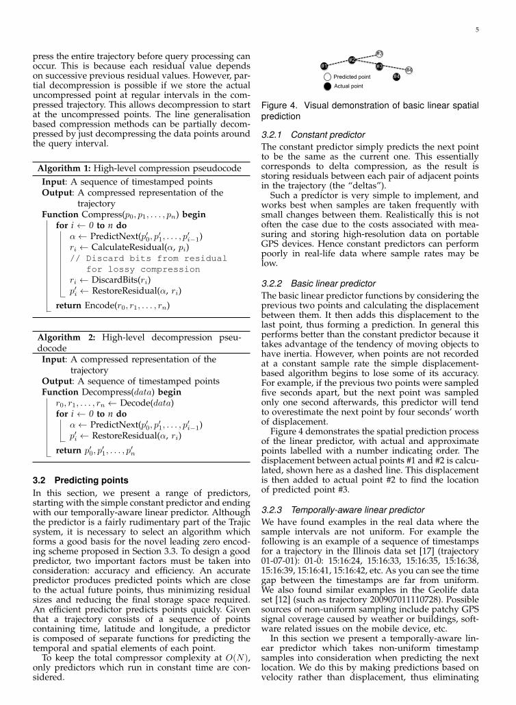
Figure 4. Visual demonstration of basic linear spatialprediction

3.2.1 Constant predictorThe constant predictor simply predicts the next pointto be the same as the current one. This essentiallycorresponds to delta compression, as the result isstoring residuals between each pair of adjacent pointsin the trajectory (the “deltas”).

Such a predictor is very simple to implement, andworks best when samples are taken frequently withsmall changes between them. Realistically this is notoften the case due to the costs associated with mea-suring and storing high-resolution data on portableGPS devices. Hence constant predictors can performpoorly in real-life data where sample rates may below.

3.2.2 Basic linear predictorThe basic linear predictor functions by considering theprevious two points and calculating the displacementbetween them. It then adds this displacement to thelast point, thus forming a prediction. In general thisperforms better than the constant predictor because ittakes advantage of the tendency of moving objects tohave inertia. However, when points are not recordedat a constant sample rate the simple displacement-based algorithm begins to lose some of its accuracy.For example, if the previous two points were sampledfive seconds apart, but the next point was sampledonly one second afterwards, this predictor will tendto overestimate the next point by four seconds’ worthof displacement.

Figure 4 demonstrates the spatial prediction processof the linear predictor, with actual and approximatepoints labelled with a number indicating order. Thedisplacement between actual points #1 and #2 is calcu-lated, shown here as a dashed line. This displacementis then added to actual point #2 to find the locationof predicted point #3.

3.2.3 Temporally-aware linear predictorWe have found examples in the real data where thesample intervals are not uniform. For example thefollowing is an example of a sequence of timestampsfor a trajectory in the Illinois data set [17] (trajectory01-07-01): 01-0: 15:16:24, 15:16:33, 15:16:35, 15:16:38,15:16:39, 15:16:41, 15:16:42, etc. As you can see the timegap between the timestamps are far from uniform.We also found similar examples in the Geolife dataset [12] (such as trajectory 200907011110728). Possiblesources of non-uniform sampling include patchy GPSsignal coverage caused by weather or buildings, soft-ware related issues on the mobile device, etc.

In this section we present a temporally-aware lin-ear predictor which takes non-uniform timestampsamples into consideration when predicting the nextlocation. We do this by making predictions based onvelocity rather than displacement, thus eliminating

6

the loss of spatial accuracy caused by a variablesample rate. In other words, using displacement onlywould result in poor prediction accuracy when thesampling rate has high variance. This is because anobject moving at constant velocity would move twiceas far if it was sampled at time tc+2∆t versus tc+∆t,where tc is the time of the current sample.

Timestamps are predicted by assuming a constantsample rate.

Time Actuallatitude

Linearprediction

Temporally-awarelinear prediction

0 0 - -

5 10 - -

6 12 20 12

8 16 14 16

Table 1Temporal awareness has a considerable impact on

the accuracy of predicted points when sample rate isnot fixed

Table 1 contains a sample set of trajectory points foran object moving with constant velocity but recordingpositions with a variable sample rate. The basic linearpredictor ignores time and assumes that the displace-ment between the second and third points will be thesame as that between the first and second. This resultsin a predicted latitude of 20, which is a considerableoverestimation of the actual latitude, 12. However,the temporally-aware linear predictor calculates thevelocity between the first and second points, assumesconstant velocity and hence accurately predicts thenext latitude to be 12. This example shows the im-portance of giving time special consideration whenforming predictions.

3.2.4 Complex predictorsThere are more complex prediction algorithms thatattempt to fit smooth curves to a group of samplepoints, including Lagrange extrapolation and naturalcubic spline extrapolation [1]. In order for the entireprediction process to run in linear time it is necessaryto only perform these more complicated predictionsbased on a fixed number of past points.

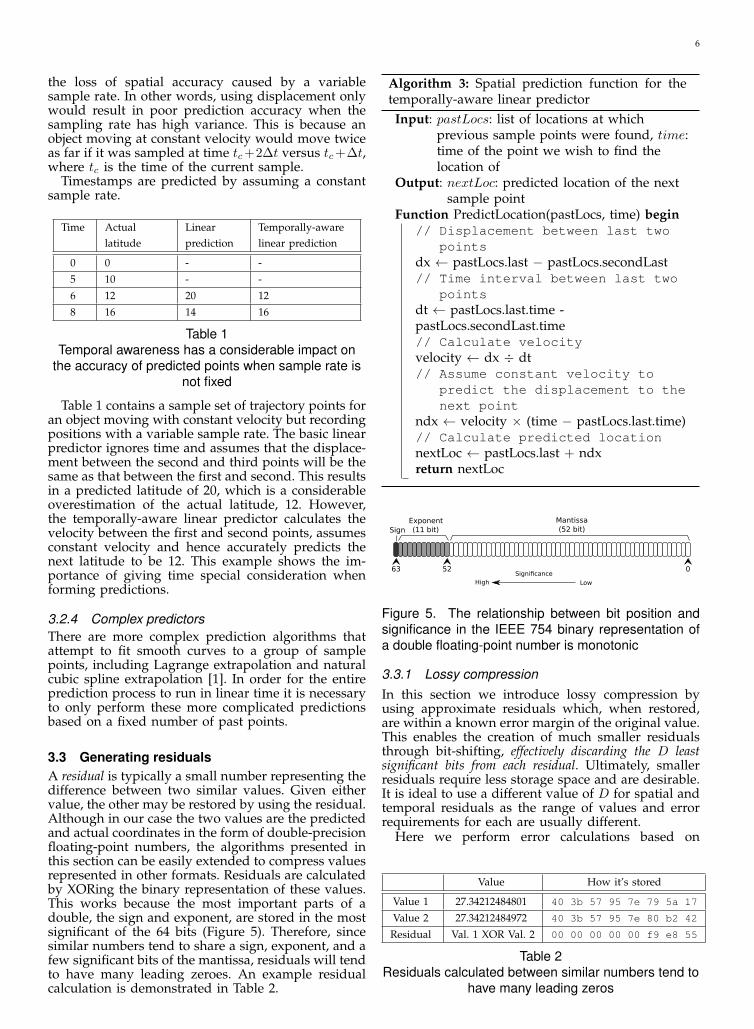
3.3 Generating residualsA residual is typically a small number representing thedifference between two similar values. Given eithervalue, the other may be restored by using the residual.Although in our case the two values are the predictedand actual coordinates in the form of double-precisionfloating-point numbers, the algorithms presented inthis section can be easily extended to compress valuesrepresented in other formats. Residuals are calculatedby XORing the binary representation of these values.This works because the most important parts of adouble, the sign and exponent, are stored in the mostsignificant of the 64 bits (Figure 5). Therefore, sincesimilar numbers tend to share a sign, exponent, and afew significant bits of the mantissa, residuals will tendto have many leading zeroes. An example residualcalculation is demonstrated in Table 2.

Algorithm 3: Spatial prediction function for thetemporally-aware linear predictorInput: pastLocs: list of locations at which

previous sample points were found, time:time of the point we wish to find thelocation of

Output: nextLoc: predicted location of the nextsample point

Function PredictLocation(pastLocs, time) begin// Displacement between last two

pointsdx ← pastLocs.last − pastLocs.secondLast// Time interval between last two

pointsdt ← pastLocs.last.time -pastLocs.secondLast.time// Calculate velocityvelocity ← dx ÷ dt// Assume constant velocity to

predict the displacement to thenext point

ndx ← velocity × (time − pastLocs.last.time)// Calculate predicted locationnextLoc ← pastLocs.last + ndxreturn nextLoc

Exponent(11 bit)Sign

Mantissa(52 bit)

63 52 0Significance

LowHigh

Figure 5. The relationship between bit position andsignificance in the IEEE 754 binary representation ofa double floating-point number is monotonic

3.3.1 Lossy compressionIn this section we introduce lossy compression byusing approximate residuals which, when restored,are within a known error margin of the original value.This enables the creation of much smaller residualsthrough bit-shifting, effectively discarding the D leastsignificant bits from each residual. Ultimately, smallerresiduals require less storage space and are desirable.It is ideal to use a different value of D for spatial andtemporal residuals as the range of values and errorrequirements for each are usually different.

Here we perform error calculations based on

Value How it’s stored

Value 1 27.34212484801 40 3b 57 95 7e 79 5a 17

Value 2 27.34212484972 40 3b 57 95 7e 80 b2 42

Residual Val. 1 XOR Val. 2 00 00 00 00 00 f9 e8 55

Table 2Residuals calculated between similar numbers tend to

have many leading zeros

7

ActualresidualPaddingHeader

l bits

p(l) bits

EO(l) bits

h bits

Figure 6. A general encoding scheme with importantbit-lengths labelled

the IEEE 754 standard for storing double-precisionfloating-point numbers, but the formulae presentedshould apply to other representations of doubles withslight modification.

It is important to ensure that the error inducedfrom the lossy compression stays within the userdefined maximum error. The maximum error possiblewhen discarding D bits from a double’s mantissa iserrormax = (2D−52 − 2−52)× 2q , where q is the valueof the double’s exponent (which in the case of theIEEE 754 standard is the number stored in the 11-bitexponent field minus an offset of 1023). In order tocalculate a safe value of D which will not exceed thespecified error bounds for the entire trajectory, it isnecessary to know the maximum exponent possiblefor values in that particular trajectory, qmax. By rear-ranging the formula we get D = blog2(errorbound ×252−qmax + 1)cqmax may be established by determining the maxi-

mum absolute value in the trajectory and performingbitwise manipulation to extract the exponent (Algo-rithm 4).

Algorithm 4: Function for calculating $D$ froma specified error bound, assuming doubles arestored using the IEEE 754 standard

Input: error: user-specified error bound, maxV al:maximum value in the trajectory

Output: D: number of bits which are safe todiscard from residuals

Function calculateDiscard(error, maxVal) begin// Extract exponent valueq ← (maxVal >> 52) & 0x7ff − 1023// Calculate safe number of bits

to discardD ← blog2(error × 252−q + 1)creturn D

3.4 Compressing residualsAlthough each residual is typically a small number,they are still technically 64-bit longs. To actuallyachieve compression, the leading zeros of the resid-uals must be compactly encoded.

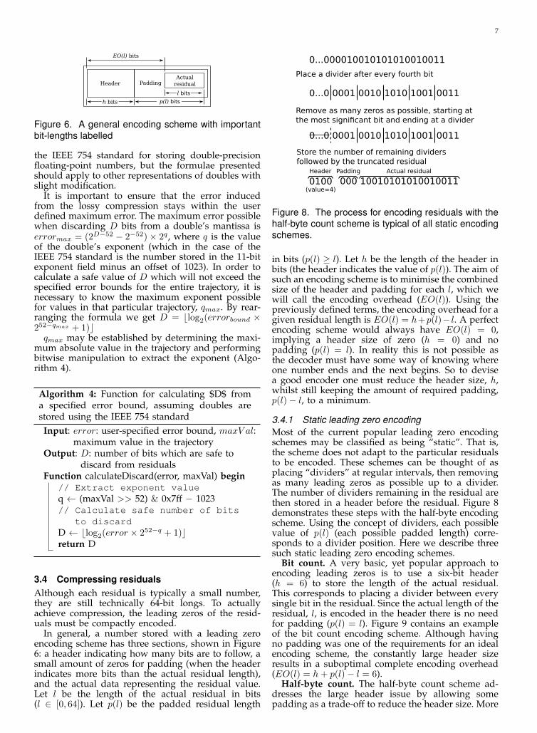
In general, a number stored with a leading zeroencoding scheme has three sections, shown in Figure6: a header indicating how many bits are to follow, asmall amount of zeros for padding (when the headerindicates more bits than the actual residual length),and the actual data representing the residual value.Let l be the length of the actual residual in bits(l ∈ [0, 64]). Let p(l) be the padded residual length

0...000010010101010010011

0...0 0001 0010 1010 1001 0011

0100 000 10010101010010011

Place a divider after every fourth bit

Remove as many zeros as possible, starting atthe most significant bit and ending at a divider

Store the number of remaining dividersfollowed by the truncated residual

Header Padding Actual residual

0...0 0001 0010 1010 1001 0011

(value=4)

Figure 8. The process for encoding residuals with thehalf-byte count scheme is typical of all static encodingschemes.

in bits (p(l) ≥ l). Let h be the length of the header inbits (the header indicates the value of p(l)). The aim ofsuch an encoding scheme is to minimise the combinedsize of the header and padding for each l, which wewill call the encoding overhead (EO(l)). Using thepreviously defined terms, the encoding overhead for agiven residual length is EO(l) = h+p(l)− l. A perfectencoding scheme would always have EO(l) = 0,implying a header size of zero (h = 0) and nopadding (p(l) = l). In reality this is not possible asthe decoder must have some way of knowing whereone number ends and the next begins. So to devisea good encoder one must reduce the header size, h,whilst still keeping the amount of required padding,p(l)− l, to a minimum.

3.4.1 Static leading zero encodingMost of the current popular leading zero encodingschemes may be classified as being “static”. That is,the scheme does not adapt to the particular residualsto be encoded. These schemes can be thought of asplacing “dividers” at regular intervals, then removingas many leading zeros as possible up to a divider.The number of dividers remaining in the residual arethen stored in a header before the residual. Figure 8demonstrates these steps with the half-byte encodingscheme. Using the concept of dividers, each possiblevalue of p(l) (each possible padded length) corre-sponds to a divider position. Here we describe threesuch static leading zero encoding schemes.

Bit count. A very basic, yet popular approach toencoding leading zeros is to use a six-bit header(h = 6) to store the length of the actual residual.This corresponds to placing a divider between everysingle bit in the residual. Since the actual length of theresidual, l, is encoded in the header there is no needfor padding (p(l) = l). Figure 9 contains an exampleof the bit count encoding scheme. Although havingno padding was one of the requirements for an idealencoding scheme, the constantly large header sizeresults in a suboptimal complete encoding overhead(EO(l) = h+ p(l)− l = 6).

Half-byte count. The half-byte count scheme ad-dresses the large header issue by allowing somepadding as a trade-off to reduce the header size. More

8

Enco

din

g

overh

ead

, EO(l)

Actual residual length, l

4

8

12

40 8 12

Bit countHalf-byte count

Byte count

16 20 24 28 32 36 40 44 48 52 56 60 64

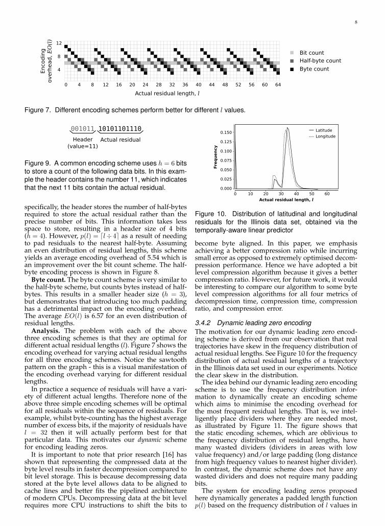
Figure 7. Different encoding schemes perform better for different l values.

001011 10101101110

Header(value=11)

Actual residual

Figure 9. A common encoding scheme uses h = 6 bitsto store a count of the following data bits. In this exam-ple the header contains the number 11, which indicatesthat the next 11 bits contain the actual residual.

specifically, the header stores the number of half-bytesrequired to store the actual residual rather than theprecise number of bits. This information takes lessspace to store, resulting in a header size of 4 bits(h = 4). However, p(l) = dl÷ 4e as a result of needingto pad residuals to the nearest half-byte. Assumingan even distribution of residual lengths, this schemeyields an average encoding overhead of 5.54 which isan improvement over the bit count scheme. The half-byte encoding process is shown in Figure 8.

Byte count. The byte count scheme is very similar tothe half-byte scheme, but counts bytes instead of half-bytes. This results in a smaller header size (h = 3),but demonstrates that introducing too much paddinghas a detrimental impact on the encoding overhead.The average EO(l) is 6.57 for an even distribution ofresidual lengths.

Analysis. The problem with each of the abovethree encoding schemes is that they are optimal fordifferent actual residual lengths (l). Figure 7 shows theencoding overhead for varying actual residual lengthsfor all three encoding schemes. Notice the sawtoothpattern on the graph - this is a visual manifestation ofthe encoding overhead varying for different residuallengths.

In practice a sequence of residuals will have a vari-ety of different actual lengths. Therefore none of theabove three simple encoding schemes will be optimalfor all residuals within the sequence of residuals. Forexample, whilst byte-counting has the highest averagenumber of excess bits, if the majority of residuals havel = 32 then it will actually perform best for thatparticular data. This motivates our dynamic schemefor encoding leading zeros.

It is important to note that prior research [16] hasshown that representing the compressed data at thebyte level results in faster decompression compared tobit level storage. This is because decompressing datastored at the byte level allows data to be aligned tocache lines and better fits the pipelined architectureof modern CPUs. Decompressing data at the bit levelrequires more CPU instructions to shift the bits to

Latitude

Longitude

Actual residual length, l

Fre

qu

en

cy

0.150

0.125

0.100

0.075

0.050

0.025

0.0000 10 20 30 40 50 60

Figure 10. Distribution of latitudinal and longitudinalresiduals for the Illinois data set, obtained via thetemporally-aware linear predictor

become byte aligned. In this paper, we emphasisachieving a better compression ratio while incurringsmall error as opposed to extremely optimised decom-pression performance. Hence we have adopted a bitlevel compression algorithm because it gives a bettercompression ratio. However, for future work, it wouldbe interesting to compare our algorithm to some bytelevel compression algorithms for all four metrics ofdecompression time, compression time, compressionratio, and compression error.

3.4.2 Dynamic leading zero encodingThe motivation for our dynamic leading zero encod-ing scheme is derived from our observation that realtrajectories have skew in the frequency distribution ofactual residual lengths. See Figure 10 for the frequencydistribution of actual residual lengths of a trajectoryin the Illinois data set used in our experiments. Noticethe clear skew in the distribution.

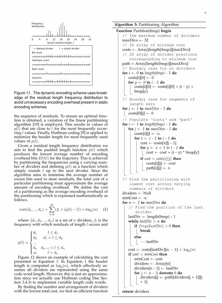
The idea behind our dynamic leading zero encodingscheme is to use the frequency distribution infor-mation to dynamically create an encoding schemewhich aims to minimise the encoding overhead forthe most frequent residual lengths. That is, we intel-ligently place dividers where they are needed most,as illustrated by Figure 11. The figure shows thatthe static encoding schemes, which are oblivious tothe frequency distribution of residual lengths, havemany wasted dividers (dividers in areas with lowvalue frequency) and/or large padding (long distancefrom high frequency values to nearest higher divider).In contrast, the dynamic scheme does not have anywasted dividers and does not require many paddingbits.

The system for encoding leading zeros proposedhere dynamically generates a padded length functionp(l) based on the frequency distribution of l values in

9

0 4 8 12 16 20 24 28 32

Frequencydistribution

Bit count

Half-byte count

Byte count

Dynamic

= Wasted divider = Useful divider

Actual residual length, l

Figure 11. The dynamic encoding scheme uses knowl-edge of the residual length frequency distribution toavoid unnecessary encoding overhead present in staticencoding schemes

the sequence of residuals. To ensure an optimal func-tion is obtained, a variation of the linear partitioningalgorithm [19] is employed. This results in values ofp(l) that are close to l for the most frequently occur-ring l values. Finally, Huffman coding [9] is applied tominimize the header length for most frequently usedvalues of p(l).

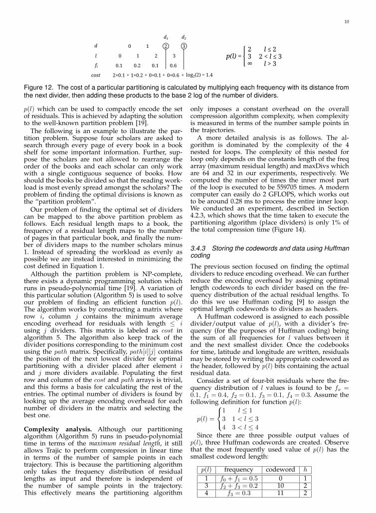
Given a residual length frequency distribution weaim to find the padded length function p(l) whichproduces the lowest average number of encodingoverhead bits EO(l) for the trajectory. This is achievedby partitioning the frequencies using a varying num-ber of dividers and defining p(l) as a function whichsimply rounds l up to the next divider. Since thealgorithm aims to minimise the average number ofexcess bits used to store residuals, the total cost of aparticular partitioning must approximate the averageamount of encoding overhead. We define the costof a partitioning as the average encoding overhead ofthe partitioning which is expressed mathematically asfollows.

cost(d1, ..., dn) =

64∑l=0

(fl × (p(l)− l)) + log2(n) (1)

where {d1, d2, ..., dn} is a set of n dividers, fl is thefrequency with which residuals of length l occurs and

p(l) =

d1 l ≤ d1d2 d1 < l ≤ d2...

dn dn−1 < l ≤ dn∞ l > dn

Figure 12 shows an example of calculating the costpresented in Equation 1. In Equation 1 the headerlength is computed as log2(n), which effectively as-sumes all dividers are represented using the samecode word length. However, this is just an approxima-tion since we actually use Huffman coding (See Sec-tion 3.4.3) to implement variable length code words.

By finding the number and arrangement of dividerswith the lowest total cost, we find an efficient function

Algorithm 5: Partitioning Algorithm

Function Partition(freqs) begin// The maximum number of dividersmaxDivs ← 32// 2D array of minimum costcosts ← Array[length(freqs)][maxDivs]// 2D array of divider positions

corresponding to minimum costpath = Array[length(freqs)][maxDivs]// Boundry case for no dividersfor i ← 0 to length(freqs) - 1 do

costs[i][0] ← 0for y ← 0 to i - 1 do

costs[i][0] ← costs[i][0] + (i - y) ×freqs[y]

// Boundry case for segments oflength zero

for j ← 1 to maxDivs - 1 docosts[0][j] ← 0

// Populate ‘costs‘ and ‘path‘for i ← 1 to length(freqs) - 1 do

for j ← 1 to maxDivs - 1 docosts[i][j] ←∞for x ← j - 1 to i - 1 do

cost ← costs[x][j - 1]for y ← x + 1 to i - 1 do

cost ← cost + (i - y) * freqs[y]

if cost < costs[i][j] thencosts[i][j] ← costpath[i][j] ← x

// Find the partitioning withlowest cost across varyingnumbers of dividers

dividers ← NullminCost ←∞for n ← 2 to maxDivs do

// Find the position of the lastdivider

lastDiv ← length(freqs) - 1while lastDiv > n do

if freqs[lastDiv] > 0 thenbreak

else−−lastDiv

cost ← costs[lastDiv][n − 1] + log2(n)if cost < minCost then

minCost ← costdividers ← Array[n]dividers[n - 1] ← lastDivfor j ← n− 2 downto 0 do

dividers[j] ← path[dividers[j + 1]][j+ 1]

return dividers

10

d

l

fl

cost

0 1 2 3

0 1 2 3

0.1 0.2 0.1 0.6

2×0.1 1×0.2 0×0.1 0×0.6+ log2(2) = 1.4+ + +

d1 d2

p(l) =l ≤ 2

2 < l ≤ 3l > 3

23∞

Figure 12. The cost of a particular partitioning is calculated by multiplying each frequency with its distance fromthe next divider, then adding these products to the base 2 log of the number of dividers.

p(l) which can be used to compactly encode the setof residuals. This is achieved by adapting the solutionto the well-known partition problem [19].

The following is an example to illustrate the par-tition problem. Suppose four scholars are asked tosearch through every page of every book in a bookshelf for some important information. Further, sup-pose the scholars are not allowed to rearrange theorder of the books and each scholar can only workwith a single contiguous sequence of books. Howshould the books be divided so that the reading work-load is most evenly spread amongst the scholars? Theproblem of finding the optimal divisions is known asthe “partition problem”.

Our problem of finding the optimal set of dividerscan be mapped to the above partition problem asfollows. Each residual length maps to a book, thefrequency of a residual length maps to the numberof pages in that particular book, and finally the num-ber of dividers maps to the number scholars minus1. Instead of spreading the workload as evenly aspossible we are instead interested in minimizing thecost defined in Equation 1.

Although the partition problem is NP-complete,there exists a dynamic programming solution whichruns in pseudo-polynomial time [19]. A variation ofthis particular solution (Algorithm 5) is used to solveour problem of finding an efficient function p(l).The algorithm works by constructing a matrix whererow i, column j contains the minimum averageencoding overhead for residuals with length ≤ iusing j dividers. This matrix is labeled as cost inalgorithm 5. The algorithm also keep track of thedivider positions corresponding to the minimum costusing the path matrix. Specifically, path[i][j] containsthe position of the next lowest divider for optimalpartitioning with a divider placed after element iand j more dividers available. Populating the firstrow and column of the cost and path arrays is trivial,and this forms a basis for calculating the rest of theentries. The optimal number of dividers is found bylooking up the average encoding overhead for eachnumber of dividers in the matrix and selecting thebest one.

Complexity analysis. Although our partitioningalgorithm (Algorithm 5) runs in pseudo-polynomialtime in terms of the maximum residual length, it stillallows Trajic to perform compression in linear timein terms of the number of sample points in eachtrajectory. This is because the partitioning algorithmonly takes the frequency distribution of residuallengths as input and therefore is independent ofthe number of sample points in the trajectory.This effectively means the partitioning algorithm

only imposes a constant overhead on the overallcompression algorithm complexity, when complexityis measured in terms of the number sample points inthe trajectories.

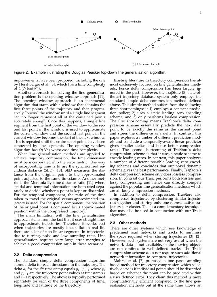
A more detailed analysis is as follows. The al-gorithm is dominated by the complexity of the 4nested for loops. The complexity of this nested forloop only depends on the constants length of the freqarray (maximum residual length) and maxDivs whichare 64 and 32 in our experiments, respectively. Wecomputed the number of times the inner most partof the loop is executed to be 559705 times. A moderncomputer can easily do 2 GFLOPS, which works outto be around 0.28 ms to process the entire inner loop.We conducted an experiment, described in Section4.2.3, which shows that the time taken to execute thepartitioning algorithm (place dividers) is only 1% ofthe total compression time (Figure 14).

3.4.3 Storing the codewords and data using Huffmancoding

The previous section focused on finding the optimaldividers to reduce encoding overhead. We can furtherreduce the encoding overhead by assigning optimallength codewords to each divider based on the fre-quency distribution of the actual residual lengths. Todo this we use Huffman coding [9] to assign theoptimal length codewords to dividers as headers.

A Huffman codeword is assigned to each possibledivider/output value of p(l), with a divider’s fre-quency (for the purposes of Huffman coding) beingthe sum of all frequencies for l values between itand the next smallest divider. Once the codebooksfor time, latitude and longitude are written, residualsmay be stored by writing the appropriate codeword asthe header, followed by p(l) bits containing the actualresidual data.

Consider a set of four-bit residuals where the fre-quency distribution of l values is found to be fo =0.1, f1 = 0.4, f2 = 0.1, f3 = 0.1, f4 = 0.3. Assume thefollowing definition for function p(l):

p(l) =

1 l ≤ 1

3 1 < l ≤ 3

4 3 < l ≤ 4Since there are three possible output values of

p(l), three Huffman codewords are created. Observethat the most frequently used value of p(l) has thesmallest codeword length:

p(l) frequency codeword h

1 f0 + f1 = 0.5 0 13 f2 + f3 = 0.2 10 24 f3 = 0.3 11 2

11

Now, to store a 2-bit residual, a header containing“10” is written out followed by 3 bits containing the2-bit residual padded with a leading zero.

4 EXPERIMENTS

4.1 Experimental setup4.1.1 Implementation and hardwareThe Trajic system and other existing compressionschemes were implemented and tested via C++11code compiled with GCC version 4.7.2 using the -O3optimization flag. Results were produced on an AMDPhenom II X4 965 processor clocked at 3.4 GHz with4 gigabytes of RAM, running Ubuntu Linux.

4.1.2 Algorithms implementedDelta compression. A simple delta compression al-gorithm was implemented with a bit-count leadingzero encoding scheme. This is the delta compressionmethod used in TrajStore [5].

TD-SED. TD-SED is a top-down line generalisationalgorithm based on the Douglas-Peucker algorithm[6] described in Section 2.1. It utilises the synchro-nised Euclidean distance (SED) as an error metricto incorporate the time dimension (as described inSection 2.1).TD-SED was used in our experiments torepresent the line generalisation approach to trajectorycompression. The reason we chose to compare againstthe Douglas-Peucker algorithm instead of others wasdue to the thorough set of experiments conductedby Muckell et al. [13]. Muckell et al. [13] comparedseven different state-of-the-art trajectory compressionalgorithms using several real data sets. The resultsshowed that Douglas-Peucker offered the best perfor-mance in terms of both low execution time and lowsynchronized Euclidean distance error.

TD-SED + Delta. TD-SED and delta compressionwere combined by first applying the line general-isation method to remove points, then storing theremaining points as a sequence of deltas.

Trajic. The Trajic system described in this paperwas implemented with the temporally-aware linearpredictor and dynamic leading zero encoding.

SQUISH. The one pass trajectory compression al-gorithm proposed by Muckell et al. [14].

Clustering compression. The clustering trajectorycompression algorithm from TrajStore[5]. The clus-tering algorithm is designed to work on partitionedregions of the 2D space. We therefore first partitionthe space into 20 x 20 grid cells of uniform width andlength. We then run the clustering algorithm on eachcell separately.

4.1.3 Data setsThe two main data sets used for the experimentswere a set of trajectories recorded by the Universityof Illinois [17] and data from the Microsoft GeoLifeproject [12].

The GeoLife data contains 17,621 trajectories (aver-age sample rate of 1 per 3 seconds and 1343 averagesamples per trajectory) taken with a variety of GPSdevices, and the set includes many modes of transportincluding walking, cycling and driving. Over 48,000

Constant Linear Temporally-aware

Mean predictiontime (ms)

0.076(0.135)

0.064(0.109)

0.084(0.138)

Mean overallresidual length

30.0 (29.7) 22.4(19.1) 22.4 (19.0)

Mean spatialresidual length

32.4 (32.0) 31.3 (27.9) 31.3 (27.8)

Mean temporalresidual length

25.4 (25.0) 4.31 (1.27) 4.30 (1.27)

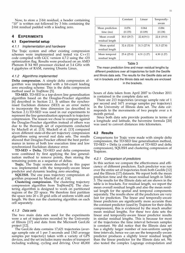
Table 3The mean prediction time and mean residual lengths by

different predictors over all trajectories for both the Geolifeand Illinois data sets. The results for the Geolife data set arenot in brackets and the Illinois data set results are enclosed

in the brackets.

hours of data taken from April 2007 to October 2011is contained in the complete data set.

There are 213 trajectories (average sample rate of 1per second and 1671 average samples per trajectory)in the University of Illinois data set. The data cor-responds to the movements of two people over a 6month period.

Since both data sets provide positions in terms ofa longitude and latitude, the haversine formula [20]was used to convert distances into kilometers.

4.2 ResultsComparisons for Trajic were made with simple deltacompression, the TD-SED line generalisation method,TD-SED + Delta (a combination of TD-SED and deltacompression), SQUISH and clustering compression ofTrajstore.

4.2.1 Comparison of predictorsIn this section we compare the effectiveness and effi-ciency of different predictors. Each predictor was runover the entire set of trajectories from both Geolife [12]and the Illinois [17] datasets. We report both the meanprediction time and the mean residual length in Table3. The results for the Illinois data set are shown in thetable is in brackets. For residual length, we report themean overall residual length and also the mean resid-ual length for the spatial and temporal componentsseparately. The results show all the predictors are veryfast for prediction. The linear and temporally-awarelinear predictors are significantly more accurate thanthe constant predictor (used by Trajstore for their deltacompression), this is evidenced by the much smallermean residual lengths. For these two data sets thelinear and temporally-aware linear predictor resultsin similar residual lengths. This is because for mostof the trajectories the time interval between samplesis constant. We did notice that the Illinois data sethas a slightly larger number of non-uniform sampletime intervals, hence we can see the temporally-awarepredictor produces a slightly lower residual lengththan the linear predictor for the Illinois data set. Wealso tested the complex Lagrange extrapolation and

12

0

1

2

3

4

5

6

0 0.2 0.4 0.6 0.8 1

Com

pres

sion

tim

e (m

s)

Compression ratio

TrajicTD-SED + Delta

TD-SED

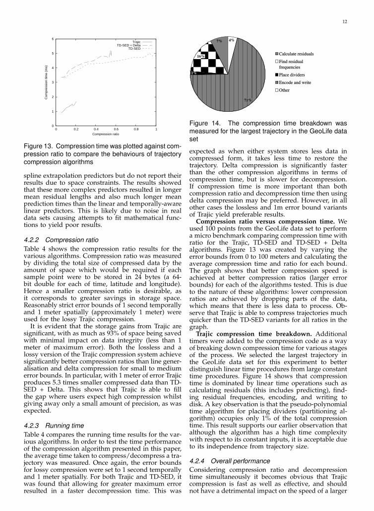
Figure 13. Compression time was plotted against com-pression ratio to compare the behaviours of trajectorycompression algorithms

spline extrapolation predictors but do not report theirresults due to space constraints. The results showedthat these more complex predictors resulted in longermean residual lengths and also much longer meanprediction times than the linear and temporally-awarelinear predictors. This is likely due to noise in realdata sets causing attempts to fit mathematical func-tions to yield poor results.

4.2.2 Compression ratioTable 4 shows the compression ratio results for thevarious algorithms. Compression ratio was measuredby dividing the total size of compressed data by theamount of space which would be required if eachsample point were to be stored in 24 bytes (a 64-bit double for each of time, latitude and longitude).Hence a smaller compression ratio is desirable, asit corresponds to greater savings in storage space.Reasonably strict error bounds of 1 second temporallyand 1 meter spatially (approximately 1 meter) wereused for the lossy Trajic compression.

It is evident that the storage gains from Trajic aresignificant, with as much as 93% of space being savedwith minimal impact on data integrity (less than 1meter of maximum error). Both the lossless and alossy version of the Trajic compression system achievesignificantly better compression ratios than line gener-alisation and delta compression for small to mediumerror bounds. In particular, with 1 meter of error Trajicproduces 5.3 times smaller compressed data than TD-SED + Delta. This shows that Trajic is able to fillthe gap where users expect high compression whilstgiving away only a small amount of precision, as wasexpected.

4.2.3 Running timeTable 4 compares the running time results for the var-ious algorithms. In order to test the time performanceof the compression algorithm presented in this paper,the average time taken to compress/decompress a tra-jectory was measured. Once again, the error boundsfor lossy compression were set to 1 second temporallyand 1 meter spatially. For both Trajic and TD-SED, itwas found that allowing for greater maximum errorresulted in a faster decompression time. This was

26/04/2014 2:18 pm

Page 1 of 1file:///Users/zhenhe/Dropbox/TrajStore%20new/Aiden/Paper-TKDE%20revision/time_breakdown%20files/time_breakdown.svg

7%

1%

71%

4%

Calculate residualsCalculate residualsFind residualFind residual frequenciesfrequenciesPlace dividersPlace dividersEncode and writeEncode and writeOtherOther

16%

Figure 14. The compression time breakdown wasmeasured for the largest trajectory in the GeoLife dataset

expected as when either system stores less data incompressed form, it takes less time to restore thetrajectory. Delta compression is significantly fasterthan the other compression algorithms in terms ofcompression time, but is slower for decompression.If compression time is more important than bothcompression ratio and decompression time then usingdelta compression may be preferred. However, in allother cases the lossless and 1m error bound variantsof Trajic yield preferable results.

Compression ratio versus compression time. Weused 100 points from the GeoLife data set to performa micro benchmark comparing compression time withratio for the Trajic, TD-SED and TD-SED + Deltaalgorithms. Figure 13 was created by varying theerror bounds from 0 to 100 meters and calculating theaverage compression time and ratio for each bound.The graph shows that better compression speed isachieved at better compression ratios (larger errorbounds) for each of the algorithms tested. This is dueto the nature of these algorithms: lower compressionratios are achieved by dropping parts of the data,which means that there is less data to process. Ob-serve that Trajic is able to compress trajectories muchquicker than the TD-SED variants for all ratios in thegraph.

Trajic compression time breakdown. Additionaltimers were added to the compression code as a wayof breaking down compression time for various stagesof the process. We selected the largest trajectory inthe GeoLife data set for this experiment to betterdistinguish linear time procedures from large constanttime procedures. Figure 14 shows that compressiontime is dominated by linear time operations such ascalculating residuals (this includes predicting), find-ing residual frequencies, encoding, and writing todisk. A key observation is that the pseudo-polynomialtime algorithm for placing dividers (partitioning al-gorithm) occupies only 1% of the total compressiontime. This result supports our earlier observation thatalthough the algorithm has a high time complexitywith respect to its constant inputs, it is acceptable dueto its independence from trajectory size.

4.2.4 Overall performanceConsidering compression ratio and decompressiontime simultaneously it becomes obvious that Trajiccompression is fast as well as effective, and shouldnot have a detrimental impact on the speed of a larger

13

AlgorithmCompression ratio Compression time (ms) Decompression time (ms)

GeoLife Illinois GeoLife Illinois GeoLife Illinois

Delta 0.55 0.39 0.7 0.3 0.8 0.4

Trajic (lossless) 0.37 0.18 5.2 2.8 0.6 0.2

TD-SED (1m error) 0.66 0.90 4.5 2.5 0.6 0.4

TD-SED + Delta (1m error) 0.37 0.36 4.3 2.5 0.6 0.3

Trajic (1m error) 0.07 0.08 1.9 1.2 0.3 0.2

TD-SED (31m error) 0.12 0.75 3.4 2.5 0.1 0.4

TD-SED + Delta (31m error) 0.07 0.31 3.0 2.6 0.1 0.3

Table 4The compression ratios and average compression/decompression times per trajectory

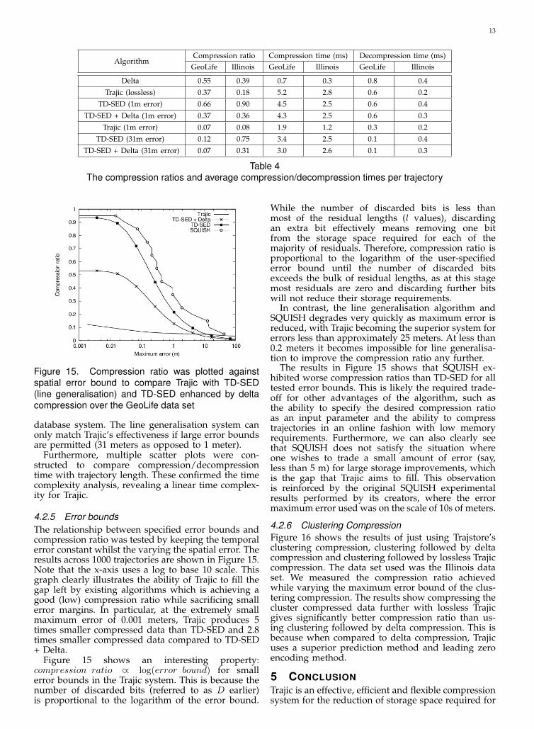
Figure 15. Compression ratio was plotted againstspatial error bound to compare Trajic with TD-SED(line generalisation) and TD-SED enhanced by deltacompression over the GeoLife data set

database system. The line generalisation system canonly match Trajic’s effectiveness if large error boundsare permitted (31 meters as opposed to 1 meter).

Furthermore, multiple scatter plots were con-structed to compare compression/decompressiontime with trajectory length. These confirmed the timecomplexity analysis, revealing a linear time complex-ity for Trajic.

4.2.5 Error boundsThe relationship between specified error bounds andcompression ratio was tested by keeping the temporalerror constant whilst the varying the spatial error. Theresults across 1000 trajectories are shown in Figure 15.Note that the x-axis uses a log to base 10 scale. Thisgraph clearly illustrates the ability of Trajic to fill thegap left by existing algorithms which is achieving agood (low) compression ratio while sacrificing smallerror margins. In particular, at the extremely smallmaximum error of 0.001 meters, Trajic produces 5times smaller compressed data than TD-SED and 2.8times smaller compressed data compared to TD-SED+ Delta.

Figure 15 shows an interesting property:compression ratio ∝ log(error bound) for smallerror bounds in the Trajic system. This is because thenumber of discarded bits (referred to as D earlier)is proportional to the logarithm of the error bound.

While the number of discarded bits is less thanmost of the residual lengths (l values), discardingan extra bit effectively means removing one bitfrom the storage space required for each of themajority of residuals. Therefore, compression ratio isproportional to the logarithm of the user-specifiederror bound until the number of discarded bitsexceeds the bulk of residual lengths, as at this stagemost residuals are zero and discarding further bitswill not reduce their storage requirements.

In contrast, the line generalisation algorithm andSQUISH degrades very quickly as maximum error isreduced, with Trajic becoming the superior system forerrors less than approximately 25 meters. At less than0.2 meters it becomes impossible for line generalisa-tion to improve the compression ratio any further.

The results in Figure 15 shows that SQUISH ex-hibited worse compression ratios than TD-SED for alltested error bounds. This is likely the required trade-off for other advantages of the algorithm, such asthe ability to specify the desired compression ratioas an input parameter and the ability to compresstrajectories in an online fashion with low memoryrequirements. Furthermore, we can also clearly seethat SQUISH does not satisfy the situation whereone wishes to trade a small amount of error (say,less than 5 m) for large storage improvements, whichis the gap that Trajic aims to fill. This observationis reinforced by the original SQUISH experimentalresults performed by its creators, where the errormaximum error used was on the scale of 10s of meters.

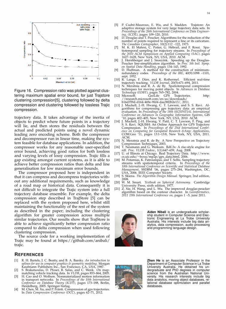
4.2.6 Clustering CompressionFigure 16 shows the results of just using Trajstore’sclustering compression, clustering followed by deltacompression and clustering followed by lossless Trajiccompression. The data set used was the Illinois dataset. We measured the compression ratio achievedwhile varying the maximum error bound of the clus-tering compression. The results show compressing thecluster compressed data further with lossless Trajicgives significantly better compression ratio than us-ing clustering followed by delta compression. This isbecause when compared to delta compression, Trajicuses a superior prediction method and leading zeroencoding method.

5 CONCLUSIONTrajic is an effective, efficient and flexible compressionsystem for the reduction of storage space required for

14

Figure 16. Compression ratio was plotted against clus-tering maximum spatial error bound, for just Trajstoreclustering compression[5], clustering followed by deltacompression and clustering followed by lossless Trajiccompression.

trajectory data. It takes advantage of the inertia ofobjects to predict where future points in a trajectorywill lie, and then stores the residuals between theactual and predicted points using a novel dynamicleading zero encoding scheme. Both the compressorand decompressor run in linear time, making the sys-tem feasible for database applications. In addition, thecompressor works for any reasonable user-specifiederror bound, achieving good ratios for both losslessand varying levels of lossy compression. Trajic fills agap existing amongst current systems, as it is able toachieve better compression ratios than delta and linegeneralisation for low maximum error bounds.

The compressor proposed here is independent inthat it can compress and decompress trajectories with-out any additional requirements, such as knowledgeof a road map or historical data. Consequently it isnot difficult to integrate the Trajic system into a fulltrajectory database ensemble. For example, the deltacompression step described in TrajStore [5] can bereplaced with the system proposed here, whilst stillmaintaining the functionality of the rest of the systemas described in the paper; including the clusteringalgorithm for greater compression across multiplesimilar trajectories. Our results show that TrajStore isable to achieve significantly better compression ratiocompared to delta compression when used followingclustering compression.

The source code for a working implementation ofTrajic may be found at https://github.com/anibali/trajic.

REFERENCES[1] R. H. Bartels, J. C. Beatty, and B. A. Barsky. An introduction to

splines for use in computer graphics & geometric modeling. MorganKaufmann Publishers Inc., San Francisco, CA, USA, 1987.

[2] S. Brakatsoulas, D. Pfoser, R. Salas, and C. Wenk. On map-matching vehicle tracking data. In VLDB, pages 853–864, 2005.

[3] H. Cao and O. Wolfson. Nonmaterialized motion informationin transport networks. In Proceedings of the 10th InternationalConference on Database Theory (ICDT), pages 173–188, Berlin,Heidelberg, 2005. Springer-Verlag.

[4] M. Chen, M. Xu, and P. Franti. Compression of gps trajectories.In Data Compression Conference (DCC), pages 62–71, 2012.

[5] P. Cudre-Mauroux, E. Wu, and S. Madden. Trajstore: Anadaptive storage system for very large trajectory data sets. InProceedings of the 26th International Conference on Data Engineer-ing, (ICDE), pages 109–120, 2010.

[6] D. Douglas and T. Peucker. Algorithms for the reduction of thenumber of points required to represent a line or its caricature.The Canadian Cartographer, 10(2):112 –122, 1973.

[7] M. K. El Mahrsi, C. Potier, G. Hebrail, and F. Rossi. Spa-tiotemporal sampling for trajectory streams. In Proceedings ofthe 2010 ACM Symposium on Applied Computing (SAC), pages1627–1628, New York, NY, USA, 2010. ACM.

[8] J. Hershberger and J. Snoeyink. Speeding up the Douglas-Peucker line-simplification algorithm. In Proc. 5th Intl. Symp.on Spatial Data Handling, pages 134–143, 1992.

[9] D. Huffman. A method for the construction of minimum-redundancy codes. Proceedings of the IRE, 40(9):1098 –1101,sept. 1952.

[10] R. Lange, F. Durr, and K. Rothermel. Efficient real-timetrajectory tracking. VLDB Journal, 20(5):671–694, 2011.

[11] N. Meratnia and R. A. de By. Spatiotemporal compressiontechniques for moving point objects. In Advances in DatabaseTechnology (EDBT), pages 765–782, 2004.

[12] Microsoft. GeoLife GPS Trajectories. http://research.microsoft.com/en-us/downloads/b16d359d-d164-469e-9fd4-daa38f2b2e13/, 2011.

[13] J. Muckell, J.-H. Hwang, C. T. Lawson, and S. S. Ravi. Al-gorithms for compressing gps trajectory data: an empiricalevaluation. In Proceedings of the 18th SIGSPATIAL InternationalConference on Advances in Geographic Information Systems, GIS’10, pages 402–405, New York, NY, USA, 2010. ACM.

[14] J. Muckell, J.-H. Hwang, V. Patil, C. T. Lawson, F. Ping, andS. S. Ravi. SQUISH: An Online Approach for GPS TrajectoryCompression. In Proceedings of the 2Nd International Confer-ence on Computing for Geospatial Research &Amp; Applications,COM.Geo ’11, pages 13:1–13:8, New York, NY, USA, 2011.ACM.

[15] N. Meratnia and R. de By. A New Perspective on TrajectoryCompression Techniques, 2003.

[16] T. Neumann and G. Weikum. Rdf-3x: A risc-style engine forrdf. Proc. VLDB Endow., 1(1):647–659, Aug. 2008.

[17] U. of Illinois at Chicago. Real Trajectory Data. http://www.cs.uic.edu/∼boxu/mp2p/gps data.html, 2006.

[18] M. Potamias, K. Patroumpas, and T. Sellis. Sampling trajectorystreams with spatiotemporal criteria. In Proceedings of the18th International Conference on Scientific and Statistical DatabaseManagement, SSDBM ’06, pages 275–284, Washington, DC,USA, 2006. IEEE Computer Society.

[19] S. Skiena. The Algorithm Design Manual. Springer, 2nd edition,2008.

[20] W. M. Smart. Textbook on Spherical Astronomy. CambridgeUniversity Press, sixth edition, 1977.

[21] Z. Xie, H. Wang, and L. Wu. The improved douglas-peuckeralgorithm based on the contour character. In Geoinformatics,2011 19th International Conference on, pages 1 –5, june 2011.

Aiden Nibali is an undergraduate scholar-ship student in Computer Science and Elec-tronic Engineering at La Trobe UniversityAustralia. His interests include big data an-alytics, data compression, audio processingand programming language design.

Zhen He is an Associate Professor in theDepartment of Computer Science in La TrobeUniversity Australia. He obtained his un-dergraduate and PhD degrees in computerscience from the Australian National Uni-versity. His research interests include bigdata analytics, moving object databases, re-lational database optimization and paralleldatabases.