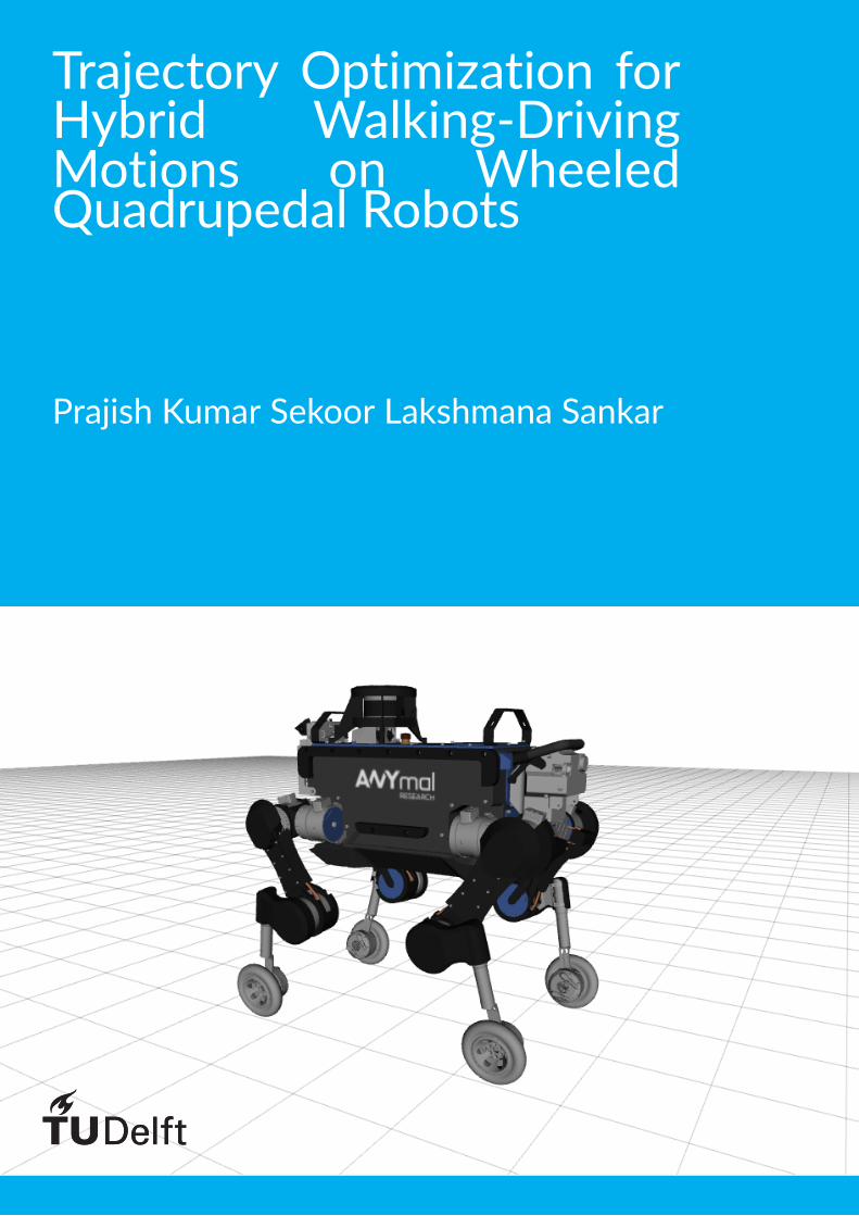
Trajectory Optimization forHybrid Walking-DrivingMotions on WheeledQuadrupedal Robots

Prajish Kumar Sekoor Lakshmana Sankar

Trajectory Optimization for HybridWalking-Driving Motions on WheeledQuadrupedal Robotsby

Prajish Kumar Sekoor Lakshmana Sankarto obtain the degree of

MASTER OF SCIENCE

at the Delft University of Technology,to be defended publicly on Tuesday October 29, 2019 at 14:00 hours.

Student number: 4743873Project duration: December 1, 2018 – August 31, 2019Supervisors: Marko Bjelonic, ETH Zürich

Prof. Dr. Marco Hutter, ETH ZürichProf. Dr.-Ing. Heike Vallery, TU Delft

Thesis committee: Prof. Dr.-Ing. Heike Vallery, TU Delft, supervisorProf. Dr. Ir. Martijn Wisse, TU DelftProf. Dr. Ir. A. J. J. (Ton) van den Boom, TU DelftProf. Dr. Ir. Arend L. Schwab, TU DelftMarko Bjelonic, ETH Zürich (external)

This thesis is confidential and cannot be made public until October 31, 2019.

An electronic version of this thesis is available at http://repository.tudelft.nl/.

Preface

My year-long association with the Robotics Systems Lab (RSL) of ETH Zürich was remarkablyinsightful and valuable than my initial expectations. I first thank Dr. Marco Hutter for the acceptance andfor arranging an internship in the last minute. Dr. Hutter also organized several events like the RoboticsSymposium, RSL Open Lab Day and the RSL summer party, which were great opportunities to networkand get a wholesome idea about the research in the lab and outside.

Marko Bjelonic was an amazing mentor in this research endeavour. Marko, who always respects mylearning curve, gave me sufficient time to navigate through the monumental pile of code and waitedpatiently for my contributions. His critical feedback, be it on writing, coding or in general, has alwaysbeen thorough; that is a great encouragement in itself. Marko and I have spent considerable timeputting some sense into the robot: dealing with punctures, smokes and some dangerous self-collisions.With every “why does it do that?" while tuning, I learnt so much with his pragmatic insights andimmediate connection to the theory. It is great to work with someone who encourages to perseverehard into one problem, while occasionally asking me to “let go and just chill by the lake". Thankyou, Marko, for that contagious excitement when the robot works and for recommending me to ANYbotics.

I am truly grateful for the involvement of Dr. Heike Vallery in this project. Her reasoning behindANYmal’s restricted turning abilities while driving, during her visit to RSL, was more concrete than myunderstanding then. With every conversation and draft review, I am surprised how much my scientificreasoning and communication improves. Thank you, Heike, for your collaboration in the paper and themotivating recommendation letter.

Some encounters in RSL, albeit brief, have helped me at the right times. Thank you, Dario, for helpingme get my gears going when I began programming. Yvain, for the useful insights into what works anddoes not on the robot. Köen, for guiding me on Delft related queries. Fabian, for helping me point outa mistake in my optimization. Thank you Christian and Péter, for introducing me to the locomotion andcontrol team of ANYbotics, where I met EV, Paco and Valentin.

My time at Zürich was way too fun, primarily because of Shruti and Vasily, who were my window tosocial life. From providing me with good food, fixing my laptop, spontaneous lake dips, hiking, partyingand biking, they have pampered me enough. Thank you, Surya, for being my go-to person for rants,advice and laughter; could not have asked for a better roommate and a best friend. Thank you, Jay;we’ve shared numerous moments of success and frustrations throughout this period. Thank you Kishan,Martina, Marti, John, Tuvshee, Anselmo and several other inmates of Tannenrauch 35. I have also beenfortunate to receive wonderful encouragements in this period from my friends in Delft: Rick, Anees,Sanjit, Aneesh, Vivek, Gokul, Sarvesh, Krishna, Ashwin, Chris, Alex, Adriana, Niels, Jens and Cathy.

I thank Gerdien for recommending me the Justus & Louise van Effen Excellence Scholarship in thefirst place and also helping in its extension.

My heartfelt gratitude goes to mom and dad for being too supportive and putting my needs beyondtheirs several times over these two years. Every time I send them a working video of the robot, theyhave always shared the same excitement as me in a follow-up call, despite asking “is this really what itis supposed to do?". Um, no papa; not really.

Finally, thank you coffee. You sustain me.

Prajish Kumar4743873Delft University of Technology29th October 2019

i

Table of ContentsI Introduction 1

II Motion Planning Overview 2

III Foot Trajectory Optimization 2III-A Preliminary definitions . . . . . . . . . . . . . . . . . . . . . . . . . . . . . . . . . 2III-B Coordinate Systems and Reference Frames . . . . . . . . . . . . . . . . . . . . . . 2III-C Parameterization of Feet Trajectories . . . . . . . . . . . . . . . . . . . . . . . . . . 3

III-C1 Swing Trajectories . . . . . . . . . . . . . . . . . . . . . . . . . . . . . . 3III-C2 Stance Trajectories . . . . . . . . . . . . . . . . . . . . . . . . . . . . . 3

III-D Formulation of Trajectory Optimization . . . . . . . . . . . . . . . . . . . . . . . . 4III-E Objectives . . . . . . . . . . . . . . . . . . . . . . . . . . . . . . . . . . . . . . . . 4

III-E1 Minimizing Accelerations . . . . . . . . . . . . . . . . . . . . . . . . . . 4III-E2 Avoid Extension of Legs During Stance . . . . . . . . . . . . . . . . . . 5III-E3 Consistent Trajectories . . . . . . . . . . . . . . . . . . . . . . . . . . . 5III-E4 Position and Velocity Soft Constraints . . . . . . . . . . . . . . . . . . . 5III-E5 Foothold Predictions . . . . . . . . . . . . . . . . . . . . . . . . . . . . . 5III-E6 General . . . . . . . . . . . . . . . . . . . . . . . . . . . . . . . . . . . . 5

III-F Equality Constraints . . . . . . . . . . . . . . . . . . . . . . . . . . . . . . . . . . . 6III-F1 Initial States . . . . . . . . . . . . . . . . . . . . . . . . . . . . . . . . . 6III-F2 Junction Constraints . . . . . . . . . . . . . . . . . . . . . . . . . . . . . 6III-F3 Foothold Constraints . . . . . . . . . . . . . . . . . . . . . . . . . . . . 6III-F4 End Constraints . . . . . . . . . . . . . . . . . . . . . . . . . . . . . . . 6

III-G Inequality Constraints . . . . . . . . . . . . . . . . . . . . . . . . . . . . . . . . . . 6III-H Switching between Hybrid Walking and Driving . . . . . . . . . . . . . . . . . . . 6

IV Base Trajectory Optimization 6IV-A Parameterization Of Base Trajectory . . . . . . . . . . . . . . . . . . . . . . . . . . 6IV-B Objectives . . . . . . . . . . . . . . . . . . . . . . . . . . . . . . . . . . . . . . . . 7IV-C Equality Constraints . . . . . . . . . . . . . . . . . . . . . . . . . . . . . . . . . . . 7IV-D Inequality Constraints . . . . . . . . . . . . . . . . . . . . . . . . . . . . . . . . . . 7

V Experimental Setup and Implementation 7V-A Setup . . . . . . . . . . . . . . . . . . . . . . . . . . . . . . . . . . . . . . . . . . . 7V-B Implementation . . . . . . . . . . . . . . . . . . . . . . . . . . . . . . . . . . . . . 8V-C Analysis . . . . . . . . . . . . . . . . . . . . . . . . . . . . . . . . . . . . . . . . . 8

VI Results and Discussions 8VI-A Gaits . . . . . . . . . . . . . . . . . . . . . . . . . . . . . . . . . . . . . . . . . . . 8VI-B Solver Times . . . . . . . . . . . . . . . . . . . . . . . . . . . . . . . . . . . . . . . 8VI-C Speed and Cost of Transportation . . . . . . . . . . . . . . . . . . . . . . . . . . . 9VI-D Reactive Behavior . . . . . . . . . . . . . . . . . . . . . . . . . . . . . . . . . . . . 9VI-E Real-World Application . . . . . . . . . . . . . . . . . . . . . . . . . . . . . . . . . 10

VII Conclusions and Future Work 11

Appendix A: ANYmal’s ability to make turns without steering the wheels 12

Appendix B: Representing the objective to avoid extension of legs in stance in QP form 12

Appendix C: Objectives for minimizing deviation from previous solution 12

Appendix D: Representing the inequality constraints term in QP form 13

Appendix E: Shifting from Driving to Walking 13

References 14

ii

List of Figures

1 Overview of the motion planning and control framework used in our work. . . . . . . . . . 22 Top view of the robot showing the coordinate systems and their corresponding reference

frames used for the foot optimization. . . . . . . . . . . . . . . . . . . . . . . . . . . . . . . 33 All possible sequences of splines for an optimization horizon of gait duration. . . . . . . . . 44 Switching between hybrid walking and pure driving. . . . . . . . . . . . . . . . . . . . . . . 65 Simulation of ANYmal on wheels while hybrid-crawling in a curve . . . . . . . . . . . . . . 86 ANYmal on wheels reacting to external force disturbances from a human. . . . . . . . . . . 107 ANYmal on wheels traversing over a wooden plank, on rough terrains and muddy under-

ground environments at the DARPA Subterranean Challenge. . . . . . . . . . . . . . . . . . 108 Measured base and feet trajectories of ANYmal at the DARPA Subterranean Challenge. . . . 119 Desired CoM and feet trajectories of ANYmal at the DARPA Subterranean Challenge while

hybrid trotting. . . . . . . . . . . . . . . . . . . . . . . . . . . . . . . . . . . . . . . . . . . . 1110 Initial configuration of ANYmal while turning. . . . . . . . . . . . . . . . . . . . . . . . . . 1211 Final configuration of ANYmal while turning. . . . . . . . . . . . . . . . . . . . . . . . . . . 12

List of Tables

I Spline durations for all possible spline sequences. . . . . . . . . . . . . . . . . . . . . . . . 4II Planning horizon and the average optimization times for different gaits. . . . . . . . . . . . . 9III Maximum heading speeds of the base, vmax, for different gaits . . . . . . . . . . . . . . . . 9IV Comparison of mechanical COT between multiple gaits . . . . . . . . . . . . . . . . . . . . 9

iii

Notations

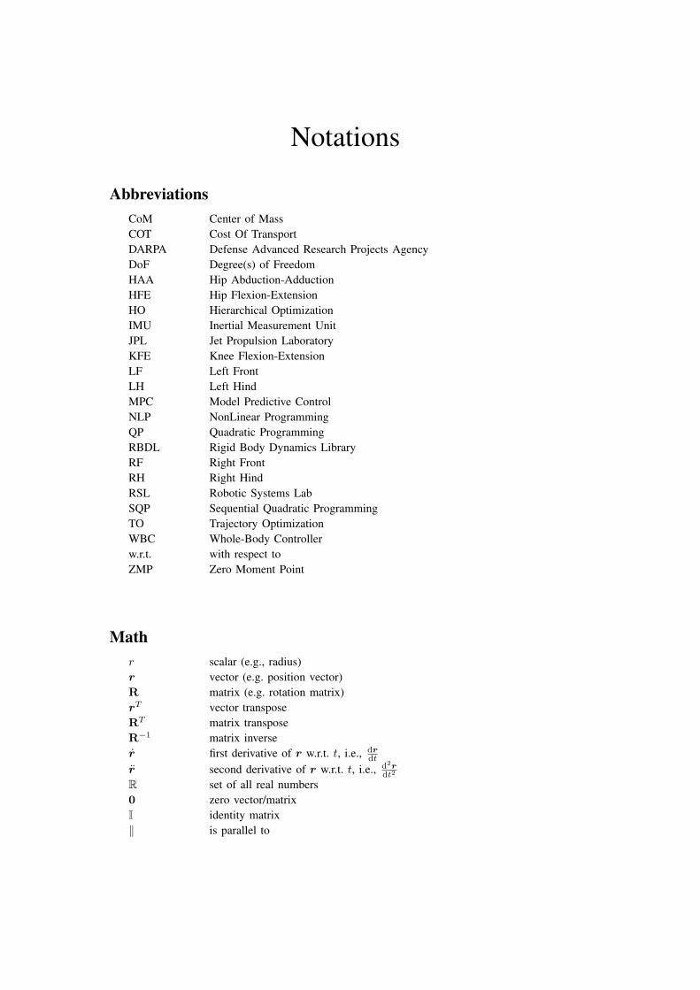
AbbreviationsCoM Center of MassCOT Cost Of TransportDARPA Defense Advanced Research Projects AgencyDoF Degree(s) of FreedomHAA Hip Abduction-AdductionHFE Hip Flexion-ExtensionHO Hierarchical OptimizationIMU Inertial Measurement UnitJPL Jet Propulsion LaboratoryKFE Knee Flexion-ExtensionLF Left FrontLH Left HindMPC Model Predictive ControlNLP NonLinear ProgrammingQP Quadratic ProgrammingRBDL Rigid Body Dynamics LibraryRF Right FrontRH Right HindRSL Robotic Systems LabSQP Sequential Quadratic ProgrammingTO Trajectory OptimizationWBC Whole-Body Controllerw.r.t. with respect toZMP Zero Moment Point

Mathr scalar (e.g., radius)r vector (e.g. position vector)R matrix (e.g. rotation matrix)rT vector transposeRT matrix transposeR−1 matrix inverser first derivative of r w.r.t. t, i.e., dr

dt

r second derivative of r w.r.t. t, i.e., d2rdt2

R set of all real numbers0 zero vector/matrixI identity matrix‖ is parallel to

iv

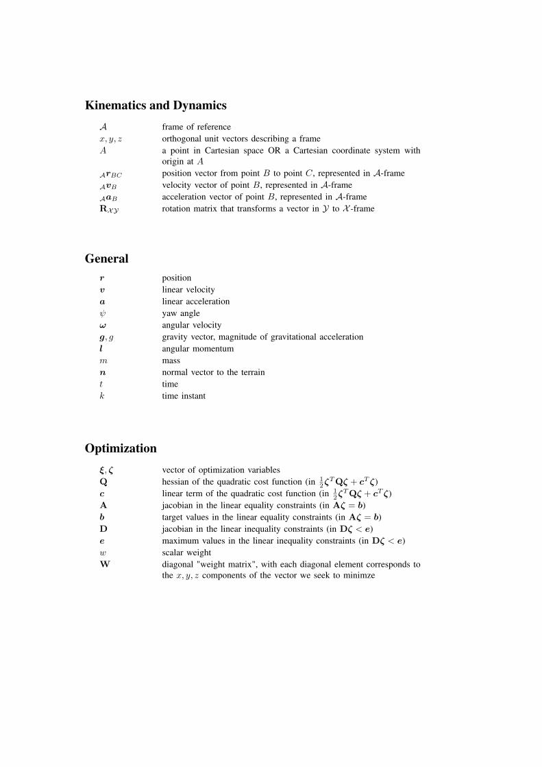
Kinematics and DynamicsA frame of referencex, y, z orthogonal unit vectors describing a frameA a point in Cartesian space OR a Cartesian coordinate system with

origin at AArBC position vector from point B to point C, represented in A-frameAvB velocity vector of point B, represented in A-frameAaB acceleration vector of point B, represented in A-frameRXY rotation matrix that transforms a vector in Y to X -frame

Generalr positionv linear velocitya linear accelerationψ yaw angleω angular velocityg, g gravity vector, magnitude of gravitational accelerationl angular momentumm massn normal vector to the terraint timek time instant

Optimizationξ, ζ vector of optimization variablesQ hessian of the quadratic cost function (in 1

2ζTQζ + cT ζ)

c linear term of the quadratic cost function (in 12ζ

TQζ + cT ζ)A jacobian in the linear equality constraints (in Aζ = b)b target values in the linear equality constraints (in Aζ = b)D jacobian in the linear inequality constraints (in Dζ < e)e maximum values in the linear inequality constraints (in Dζ < e)w scalar weightW diagonal "weight matrix", with each diagonal element corresponds to

the x, y, z components of the vector we seek to minimze

v

Relevant Publication

Marko Bjelonic, Prajish K. Sankar, Carmine D. Bellicoso, Heike Vallery and Marco Hutter. Rollingin the Deep - Hybrid Locomotion for Wheeled-Legged Robots using Online Trajectory Optimization.Submitted to IEEE Robotics and Automation Letters, 2020.

Please cite as

@article{bjelonic2020rolling,author = {Bjelonic, Marko and

Sankar, Prajish K. andBellicoso, Carmine D andVallery, Heike andHutter, Marco},

title = {Rolling in the Deep - Hybrid Locomotion for Wheeled-LeggedRobots using Online Trajectory Optimization},

journal = {submitted to IEEE Robotics and Automation Letters},year = {2020}

}

Paper: https://arxiv.org/abs/1909.07193Video: https://www.youtube.com/watch?v=ukY0vyM-yfY

vi

Abstract

Wheeled-legged (hybrid) robots have the potential for highly agile and versatile locomotion in anyreal-world application requiring rapid, long-distance mobility skills on challenging terrain. The abilityto walk and drive simultaneously is an attractive feature of these hybrid systems, but is unexplored inliterature.

This report presents an online trajectory optimization framework for high-dimensional wheeled-leggedquadrupedal robots where the feet and base trajectories are generated in a model predictive controlfashion for robustness against disturbances. Our feet optimization employs a unique parameterizationthat captures the velocity constraints of the wheels’ rolling and our base optimization uses a ZMP-basedbalance criterion.

Our approach is verified on a torque-controlled quadrupedal robot with nonsteerable wheels. Therobot performs hybrid locomotion with different gait sequences on flat and rough terrain. Moreover,our optimization framework generates base trajectories at a rate of about 100 Hz and feet trajectoriesat 1000 Hz or higher. In addition, we validated the robotic platform at the Defense Advanced ResearchProjects Agency (DARPA) Subterranean Challenge, where the robot rapidly maps, navigates, and exploresdynamic underground environments.

vii

viii

ME51032 ME-BMD MSc ProjectStudent Number 4743873

Trajectory Optimization for Hybrid Walking-DrivingMotions on Wheeled Quadrupedal Robots

Prajish Kumar Sankar1, Marko Bjelonic2, Heike Vallery1 and Marco Hutter2

Abstract—Wheeled-legged (hybrid) robots have the potentialfor highly agile and versatile locomotion in any real-worldapplication requiring rapid, long-distance mobility skills onchallenging terrain. The ability to walk and drive simultaneouslyis an attractive feature of these hybrid systems, but is unexploredin literature.

This report presents an online trajectory optimization frame-work for high-dimensional wheeled-legged quadrupedal robotswhere the feet and base trajectories are generated in a modelpredictive control fashion for robustness against disturbances.Our feet optimization employs a unique parameterization thatcaptures the velocity constraints of the wheels’ rolling and ourbase optimization uses a ZMP-based balance criterion.

Our approach is verified on a torque-controlled quadrupedalrobot with nonsteerable wheels. The robot performs hybridlocomotion with different gait sequences on flat and roughterrain. Moreover, our optimization framework generates basetrajectories at a rate of about 100 Hz and feet trajectoriesat 1000 Hz or higher. In addition, we validated the roboticplatform at the Defense Advanced Research Projects Agency(DARPA) Subterranean Challenge, where the robot rapidly maps,navigates, and explores dynamic underground environments.

I. INTRODUCTION

LEGGED robotic systems, on one end, are dexterousenough to navigate in tight spaces and accept terrain

discontinuities like gaps, stairs and minor obstacles [1], [2].On the other end, wheeled mobile robots are an excellentchoice for fast locomotion, whose control strategies are fairlyestablished [3]. The recent interest in combining the benefitsof both has resulted in hybrid robots1, which can drive fast onflat terrains and use legged locomotion on rough surfaces.

Compared with traditional legged robots, some hybrid sys-tems have broken speed records and reduced cost of trans-portation [4]–[6]. Compared with traditional wheeled vehicles,hybrid systems in literature have demonstrated three mainadvantages. First, the legs can be used as mechanisms to varyfootprints for navigating tight spaces without losing balance.Second, the legs can provide suspension for traversing ruggedterrains. Most hybrid systems in literature demonstrate justthese two benefits [7]–[19].

1P.K. Sankar and H. Vallery are with Mechanical, Maritimeand Materials Engineering (3mE), TU Delft, 2628 CD Delft,Netherlands (email: P.K.Sankar@student.tudelft.nl,h.vallery@tudelft.nl).

2M. Bjelonic and M. Hutter are with the Robotic Sys-tems Lab, ETH Zürich, 8092 Zürich, Switzerland (email:marko.bjelonic@mavt.ethz.ch, mahutter@ethz.ch).

1Here, we use "hybrid systems" to refer to robots with wheels connectedto the main body through extendable/retractable legs.

A few studies have demonstrated the third advantage: theability to step over obstacles larger than the wheels’ radius.A wheeled hexapod in [20] was one of the earliest worksto demonstrate walking over large obstacles, but could notbe used on-the-fly due to relatively inefficient computations.Walking in [21] was implemented by turning the plane ofwheels so that they lay flat on the surface terrain; whichis unnecessary considering that the rotation of the wheelscould be merely controlled. Some recent works on quadrupedalrobots like CENTAURO [22], [23], Momaro [24], [25] andANYmal [4], [26] have shown impressive results. All thesesystems demonstrate both driving and walking, but not bothsimultaneously; the locomotion modes are manually switcheddepending on the need.

The full exploitation of hybrid systems would be hybridmotions where the system drives and walks at the sametime. Examples include ice skating and roller skating [5].These hybrid motions, however, are relatively unexplored inliterature. Skaterbots [27] is an example, but the nonlinearprogramming (NLP) involved can suffer from the curse ofdimensionality when employed on a quadrupedal system withhigher degrees of freedom (DoF). Boston Dynamic’s Handle[28] is an inspiration but lacks supporting publication.

Motion planning for quadrupedal robots requires generatingtrajectories for both the feet and the base (torso). Thesetrajectories can be either predesigned, generated based onsimple heuristics or using optimal control problems. ForANYmal [29] on skates [5], these trajectories are hand-crafted,and hence the robot is generally not robust. In ANYmal’sfirst attempt with actuated wheels [4], the trajectories for thedriving motion are generated based on simple heuristics, likevelocity projections. This approach works for driving, butcannot be easily extended to hybrid motions.

Trajectory generation by solving an optimal control problemis pervasive and recommended in the literature. Tools liketrajectory optimization (TO) and model predictive control(MPC) have produced reliable and robust motions, even forblind locomotion on rough terrains [30]. Currently, only [26]tackles planning through TO for hybrid motions in ANYmalon wheels, while incorporating the rolling constraints in theframework. The approach involves generating trajectories forboth feet (wheels) and the base in the same optimizationproblem. This, however, resulted in a slower computationthan in [4]. Additionally, the results were verified only ona simulation, and therefore, the extension of their frameworkto the real robot is unknown.

ANYmal [29] is significantly different from other wheeledquadrupedal robots in literature because the wheels are non-

2 ME51032 ME-BMD MSC PROJECT, OCTOBER 2019

steerable. The orientation of wheels with respect to (w.r.t.)base follows a sequence of rotations corresponding to hipad/abduction, hip flex/extension and knee flex/extension2; noendo/exo rotation joint exists for steering. Therefore, ANYmalcan only perform small turns while driving. For larger turnangles, the robot must lift its legs and place them somewherecloser, so that the legs do not get overextended. The reasoningbehind small turns is in Appendix A.

In this report, we provide a TO framework for hybridmotions on ANYmal on wheels. The framework involvessequential generation of feet and base trajectories in separateoptimization problems. We verify the framework on the robotby employing multiple walking gaits with high-speed driving.To the best of our knowledge, this is the first proven attemptof hybrid motions with nonsteerable wheels employed oversuch a wide range of walking gaits.

II. MOTION PLANNING OVERVIEW

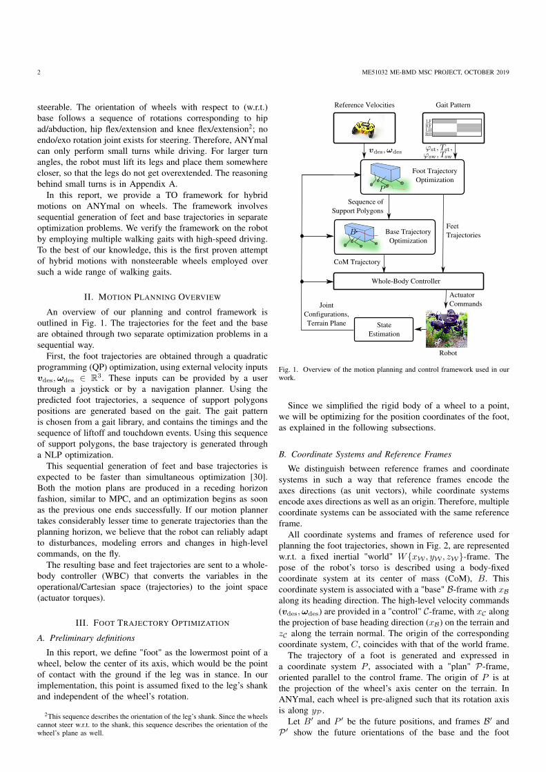
An overview of our planning and control framework isoutlined in Fig. 1. The trajectories for the feet and the baseare obtained through two separate optimization problems in asequential way.

First, the foot trajectories are obtained through a quadraticprogramming (QP) optimization, using external velocity inputsvdes,ωdes ∈ R3. These inputs can be provided by a userthrough a joystick or by a navigation planner. Using thepredicted foot trajectories, a sequence of support polygonspositions are generated based on the gait. The gait patternis chosen from a gait library, and contains the timings and thesequence of liftoff and touchdown events. Using this sequenceof support polygons, the base trajectory is generated througha NLP optimization.

This sequential generation of feet and base trajectories isexpected to be faster than simultaneous optimization [30].Both the motion plans are produced in a receding horizonfashion, similar to MPC, and an optimization begins as soonas the previous one ends successfully. If our motion plannertakes considerably lesser time to generate trajectories than theplanning horizon, we believe that the robot can reliably adaptto disturbances, modeling errors and changes in high-levelcommands, on the fly.

The resulting base and feet trajectories are sent to a whole-body controller (WBC) that converts the variables in theoperational/Cartesian space (trajectories) to the joint space(actuator torques).

III. FOOT TRAJECTORY OPTIMIZATION

A. Preliminary definitions

In this report, we define "foot" as the lowermost point of awheel, below the center of its axis, which would be the pointof contact with the ground if the leg was in stance. In ourimplementation, this point is assumed fixed to the leg’s shankand independent of the wheel’s rotation.

2This sequence describes the orientation of the leg’s shank. Since the wheelscannot steer w.r.t. to the shank, this sequence describes the orientation of thewheel’s plane as well.

Reference Velocities Gait Pattern

Foot TrajectoryOptimization

Base Trajectory Optimization

Whole-Body Controller

Sequence ofSupport Polygons

CoM Trajectory

State Estimation

Joint Configurations, Terrain Plane

Robot

Actuator Commands

Feet Trajectories

Fig. 1. Overview of the motion planning and control framework used in ourwork.

Since we simplified the rigid body of a wheel to a point,we will be optimizing for the position coordinates of the foot,as explained in the following subsections.

B. Coordinate Systems and Reference Frames

We distinguish between reference frames and coordinatesystems in such a way that reference frames encode theaxes directions (as unit vectors), while coordinate systemsencode axes directions as well as an origin. Therefore, multiplecoordinate systems can be associated with the same referenceframe.

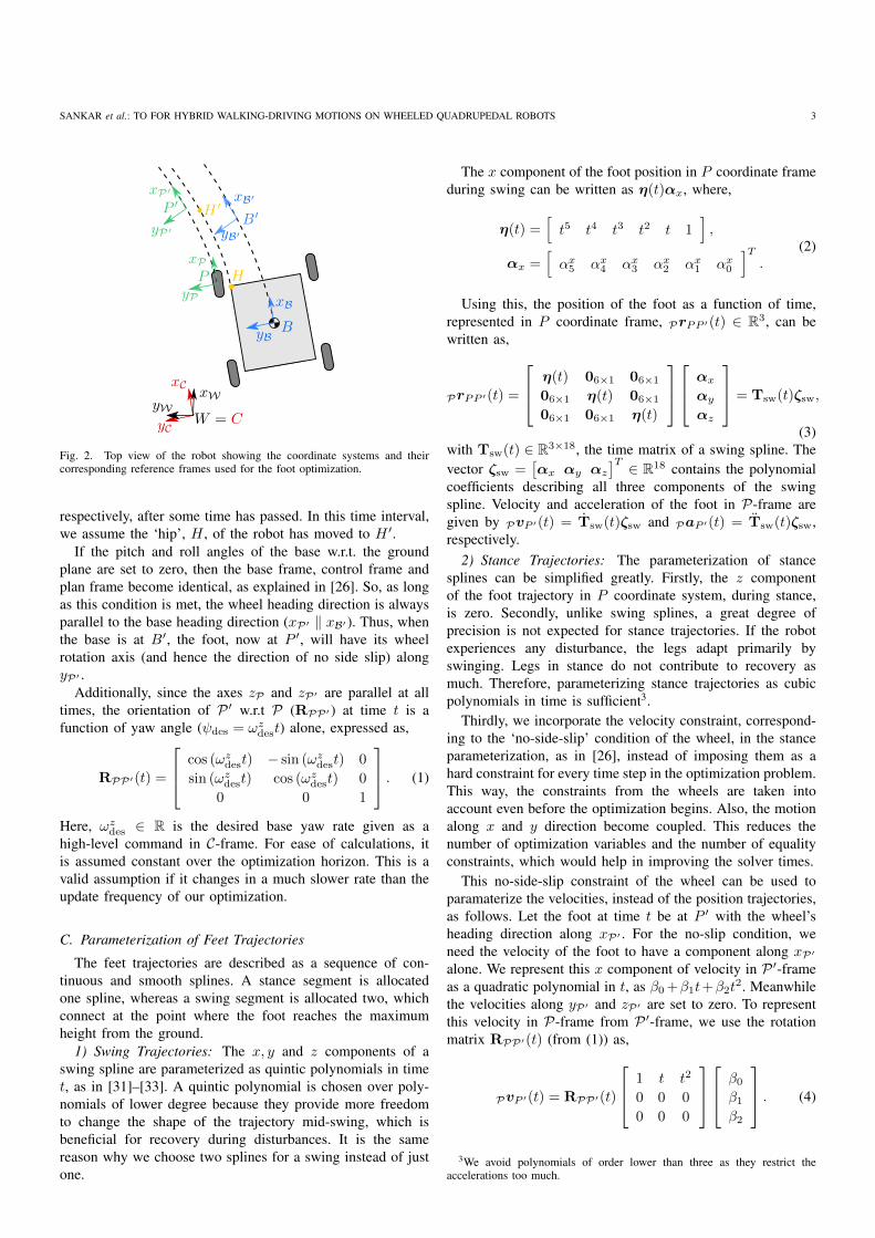
All coordinate systems and frames of reference used forplanning the foot trajectories, shown in Fig. 2, are representedw.r.t. a fixed inertial "world" W{xW , yW , zW}-frame. Thepose of the robot’s torso is described using a body-fixedcoordinate system at its center of mass (CoM), B. Thiscoordinate system is associated with a "base" B-frame with xBalong its heading direction. The high-level velocity commands(vdes,ωdes) are provided in a "control" C-frame, with xC alongthe projection of base heading direction (xB) on the terrain andzC along the terrain normal. The origin of the correspondingcoordinate system, C, coincides with that of the world frame.

The trajectory of a foot is generated and expressed ina coordinate system P , associated with a "plan" P-frame,oriented parallel to the control frame. The origin of P is atthe projection of the wheel’s axis center on the terrain. InANYmal, each wheel is pre-aligned such that its rotation axisis along yP .

Let B′ and P ′ be the future positions, and frames B′ andP ′ show the future orientations of the base and the foot

SANKAR et al.: TO FOR HYBRID WALKING-DRIVING MOTIONS ON WHEELED QUADRUPEDAL ROBOTS 3

Fig. 2. Top view of the robot showing the coordinate systems and theircorresponding reference frames used for the foot optimization.

respectively, after some time has passed. In this time interval,we assume the ‘hip’, H , of the robot has moved to H ′.

If the pitch and roll angles of the base w.r.t. the groundplane are set to zero, then the base frame, control frame andplan frame become identical, as explained in [26]. So, as longas this condition is met, the wheel heading direction is alwaysparallel to the base heading direction (xP′ ‖ xB′ ). Thus, whenthe base is at B′, the foot, now at P ′, will have its wheelrotation axis (and hence the direction of no side slip) alongyP′ .

Additionally, since the axes zP and zP′ are parallel at alltimes, the orientation of P ′ w.r.t P (RPP′ ) at time t is afunction of yaw angle (ψdes = ωz

dest) alone, expressed as,

RPP′(t) =

cos (ωzdest) − sin (ωz

dest) 0

sin (ωzdest) cos (ωz

dest) 0

0 0 1

. (1)

Here, ωzdes ∈ R is the desired base yaw rate given as a

high-level command in C-frame. For ease of calculations, itis assumed constant over the optimization horizon. This is avalid assumption if it changes in a much slower rate than theupdate frequency of our optimization.

C. Parameterization of Feet Trajectories

The feet trajectories are described as a sequence of con-tinuous and smooth splines. A stance segment is allocatedone spline, whereas a swing segment is allocated two, whichconnect at the point where the foot reaches the maximumheight from the ground.

1) Swing Trajectories: The x, y and z components of aswing spline are parameterized as quintic polynomials in timet, as in [31]–[33]. A quintic polynomial is chosen over poly-nomials of lower degree because they provide more freedomto change the shape of the trajectory mid-swing, which isbeneficial for recovery during disturbances. It is the samereason why we choose two splines for a swing instead of justone.

The x component of the foot position in P coordinate frameduring swing can be written as η(t)αx, where,

η(t) =[t5 t4 t3 t2 t 1

],

αx =[αx

5 αx4 αx

3 αx2 αx

1 αx0

]T.

(2)

Using this, the position of the foot as a function of time,represented in P coordinate frame, PrPP ′(t) ∈ R3, can bewritten as,

PrPP ′(t) =

η(t) 06×1 06×1

06×1 η(t) 06×1

06×1 06×1 η(t)

αx

αy

αz

= Tsw(t)ζsw,

(3)with Tsw(t) ∈ R3×18, the time matrix of a swing spline. Thevector ζsw =

[αx αy αz

]T ∈ R18 contains the polynomialcoefficients describing all three components of the swingspline. Velocity and acceleration of the foot in P-frame aregiven by PvP ′(t) = Tsw(t)ζsw and PaP ′(t) = Tsw(t)ζsw,respectively.

2) Stance Trajectories: The parameterization of stancesplines can be simplified greatly. Firstly, the z componentof the foot trajectory in P coordinate system, during stance,is zero. Secondly, unlike swing splines, a great degree ofprecision is not expected for stance trajectories. If the robotexperiences any disturbance, the legs adapt primarily byswinging. Legs in stance do not contribute to recovery asmuch. Therefore, parameterizing stance trajectories as cubicpolynomials in time is sufficient3.

Thirdly, we incorporate the velocity constraint, correspond-ing to the ‘no-side-slip’ condition of the wheel, in the stanceparameterization, as in [26], instead of imposing them as ahard constraint for every time step in the optimization problem.This way, the constraints from the wheels are taken intoaccount even before the optimization begins. Also, the motionalong x and y direction become coupled. This reduces thenumber of optimization variables and the number of equalityconstraints, which would help in improving the solver times.

This no-side-slip constraint of the wheel can be used toparamaterize the velocities, instead of the position trajectories,as follows. Let the foot at time t be at P ′ with the wheel’sheading direction along xP′ . For the no-slip condition, weneed the velocity of the foot to have a component along xP′

alone. We represent this x component of velocity in P ′-frameas a quadratic polynomial in t, as β0 +β1t+β2t

2. Meanwhilethe velocities along yP′ and zP′ are set to zero. To representthis velocity in P-frame from P ′-frame, we use the rotationmatrix RPP′(t) (from (1)) as,

PvP ′(t) = RPP′(t)

1 t t2

0 0 0

0 0 0

β0

β1

β2

. (4)

3We avoid polynomials of order lower than three as they restrict theaccelerations too much.

4 ME51032 ME-BMD MSC PROJECT, OCTOBER 2019

To get the foot trajectory, we integrate this velocity w.r.t tand add the initial position [xinit yinit 0]T as,

PrPP ′(t) =

xinit

yinit

0

+

t∫0

PvP ′(t)dt. (5)

Assuming ωzdes is constant over the optimization horizon,

the integration is solved analytically. The resulting expressionis,

PrPP ′(t) = Tst(ωzdes, t)ζst, (6)

where, Tst(ωzdes, t) ∈ R3×5 is the time matrix of the stance

spline and the vector ζst = [β0 β1 β2 xinit yinit]T ∈ R5

contains the polynomial coefficients that describes this stancespline.

Unlike in swing, the position of the foot in stance attime t depends on ωz

des too. For brevity and consistency,we write the foot trajectories in stance as PrPP ′(t), insteadof PrPP ′(ωz

des, t). For negligible base yaw rates,∣∣ωz

des

∣∣ <10−5 rad/s, we use the time matrix of the limiting case,Tst(t) = lim

ωzdes→0

Tst(ωzdes, t).

D. Formulation of Trajectory Optimization

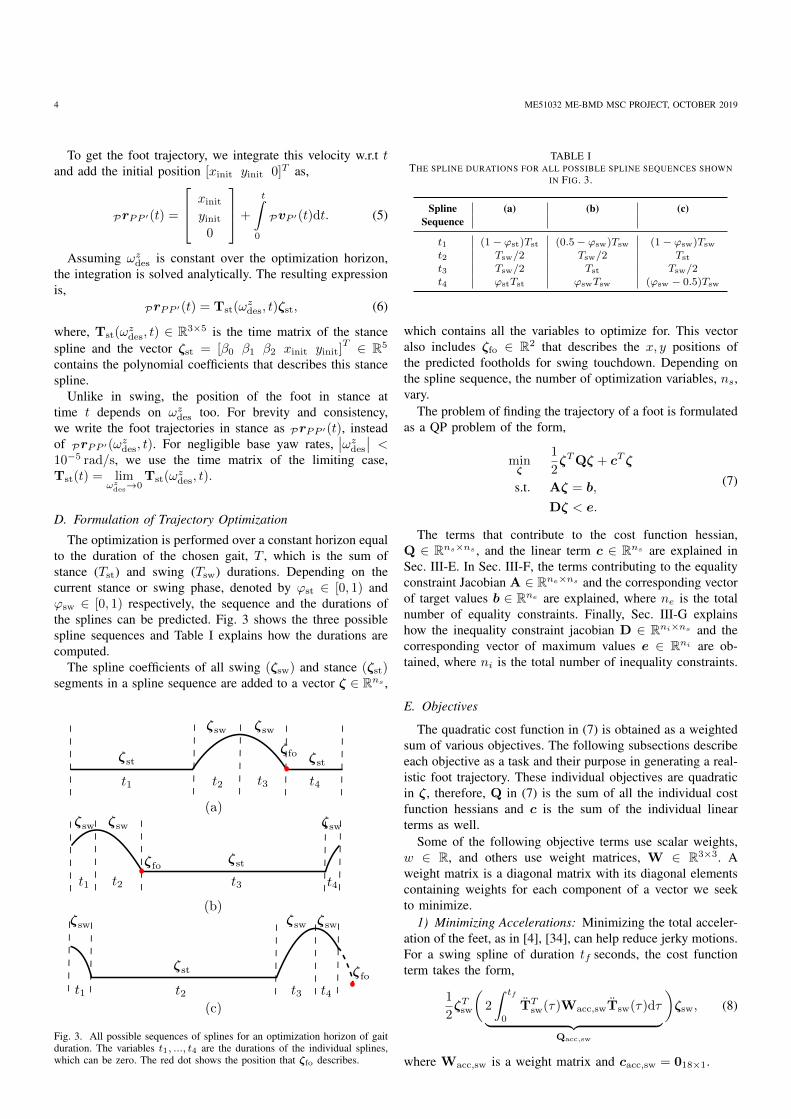
The optimization is performed over a constant horizon equalto the duration of the chosen gait, T , which is the sum ofstance (Tst) and swing (Tsw) durations. Depending on thecurrent stance or swing phase, denoted by ϕst ∈ [0, 1) andϕsw ∈ [0, 1) respectively, the sequence and the durations ofthe splines can be predicted. Fig. 3 shows the three possiblespline sequences and Table I explains how the durations arecomputed.

The spline coefficients of all swing (ζsw) and stance (ζst)segments in a spline sequence are added to a vector ζ ∈ Rns ,

Fig. 3. All possible sequences of splines for an optimization horizon of gaitduration. The variables t1, ..., t4 are the durations of the individual splines,which can be zero. The red dot shows the position that ζfo describes.

TABLE ITHE SPLINE DURATIONS FOR ALL POSSIBLE SPLINE SEQUENCES SHOWN

IN FIG. 3.

Spline (a) (b) (c)Sequence

t1 (1− ϕst)Tst (0.5− ϕsw)Tsw (1− ϕsw)Tsw

t2 Tsw/2 Tsw/2 Tst

t3 Tsw/2 Tst Tsw/2

t4 ϕstTst ϕswTsw (ϕsw − 0.5)Tsw

which contains all the variables to optimize for. This vectoralso includes ζfo ∈ R2 that describes the x, y positions ofthe predicted footholds for swing touchdown. Depending onthe spline sequence, the number of optimization variables, ns,vary.

The problem of finding the trajectory of a foot is formulatedas a QP problem of the form,

minζ

1

2ζTQζ + cT ζ

s.t. Aζ = b,

Dζ < e.

(7)

The terms that contribute to the cost function hessian,Q ∈ Rns×ns , and the linear term c ∈ Rns are explained inSec. III-E. In Sec. III-F, the terms contributing to the equalityconstraint Jacobian A ∈ Rne×ns and the corresponding vectorof target values b ∈ Rne are explained, where ne is the totalnumber of equality constraints. Finally, Sec. III-G explainshow the inequality constraint jacobian D ∈ Rni×ns and thecorresponding vector of maximum values e ∈ Rni are ob-tained, where ni is the total number of inequality constraints.

E. Objectives

The quadratic cost function in (7) is obtained as a weightedsum of various objectives. The following subsections describeeach objective as a task and their purpose in generating a real-istic foot trajectory. These individual objectives are quadraticin ζ, therefore, Q in (7) is the sum of all the individual costfunction hessians and c is the sum of the individual linearterms as well.

Some of the following objective terms use scalar weights,w ∈ R, and others use weight matrices, W ∈ R3×3. Aweight matrix is a diagonal matrix with its diagonal elementscontaining weights for each component of a vector we seekto minimize.

1) Minimizing Accelerations: Minimizing the total acceler-ation of the feet, as in [4], [34], can help reduce jerky motions.For a swing spline of duration tf seconds, the cost functionterm takes the form,

1

2ζTsw

(2

∫ tf

0

TTsw(τ)Wacc,swTsw(τ)dτ︸ ︷︷ ︸

Qacc,sw

)ζsw, (8)

where Wacc,sw is a weight matrix and cacc,sw = 018×1.

SANKAR et al.: TO FOR HYBRID WALKING-DRIVING MOTIONS ON WHEELED QUADRUPEDAL ROBOTS 5

For a stance segment with duration tf , we follow a similarformulation with a weight matrix Wacc,st as,

1

2ζTst

(2

∫ tf

0

TTst(ω

zdes, τ)Wacc,stTst(ω

zdes, τ)dτ︸ ︷︷ ︸

Qacc,st

)ζst, (9)

with cacc,st = 018×1 as well.2) Avoid Extension of Legs During Stance: During stance,

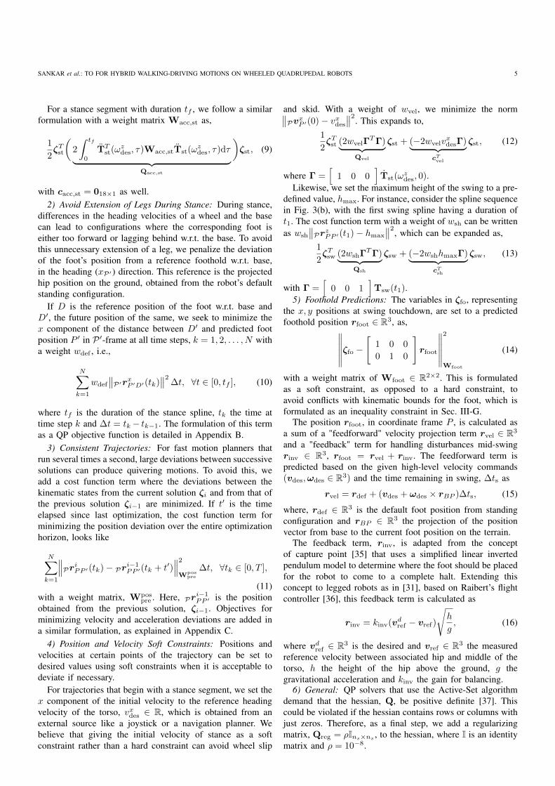
differences in the heading velocities of a wheel and the basecan lead to configurations where the corresponding foot iseither too forward or lagging behind w.r.t. the base. To avoidthis unnecessary extension of a leg, we penalize the deviationof the foot’s position from a reference foothold w.r.t. base,in the heading (xP′ ) direction. This reference is the projectedhip position on the ground, obtained from the robot’s defaultstanding configuration.

If D is the reference position of the foot w.r.t. base andD′, the future position of the same, we seek to minimize thex component of the distance between D′ and predicted footposition P ′ in P ′-frame at all time steps, k = 1, 2, . . . , N witha weight wdef , i.e.,

N∑k=1

wdef

∥∥P′rxP ′D′(tk)∥∥2

∆t, ∀t ∈ [0, tf ], (10)

where tf is the duration of the stance spline, tk the time attime step k and ∆t = tk− tk−1. The formulation of this termas a QP objective function is detailed in Appendix B.

3) Consistent Trajectories: For fast motion planners thatrun several times a second, large deviations between successivesolutions can produce quivering motions. To avoid this, weadd a cost function term where the deviations between thekinematic states from the current solution ζi and from that ofthe previous solution ζi−1 are minimized. If t′ is the timeelapsed since last optimization, the cost function term forminimizing the position deviation over the entire optimizationhorizon, looks like

N∑k=1

∥∥∥PriPP ′(tk)− Pri−1PP ′(tk + t′)

∥∥∥2

Wpospre

∆t, ∀tk ∈ [0, T ],

(11)with a weight matrix, Wpos

pre . Here, Pri−1PP ′ is the position

obtained from the previous solution, ζi−1. Objectives forminimizing velocity and acceleration deviations are added ina similar formulation, as explained in Appendix C.

4) Position and Velocity Soft Constraints: Positions andvelocities at certain points of the trajectory can be set todesired values using soft constraints when it is acceptable todeviate if necessary.

For trajectories that begin with a stance segment, we set thex component of the initial velocity to the reference headingvelocity of the torso, vxdes ∈ R, which is obtained from anexternal source like a joystick or a navigation planner. Webelieve that giving the initial velocity of stance as a softconstraint rather than a hard constraint can avoid wheel slip

and skid. With a weight of wvel, we minimize the norm∥∥PvxP ′(0)− vxdes

∥∥2. This expands to,

1

2ζTst (2wvelΓ

TΓ)︸ ︷︷ ︸Qvel

ζst + (−2wvelvxdesΓ)︸ ︷︷ ︸

cTvel

ζst, (12)

where Γ =[

1 0 0]

Tst(ωzdes, 0).

Likewise, we set the maximum height of the swing to a pre-defined value, hmax. For instance, consider the spline sequencein Fig. 3(b), with the first swing spline having a duration oft1. The cost function term with a weight of wsh can be writtenas wsh

∥∥PrzPP ′(t1)− hmax

∥∥2, which can be expanded as,

1

2ζTsw (2wshΓTΓ)︸ ︷︷ ︸

Qsh

ζsw + (−2wshhmaxΓ)︸ ︷︷ ︸cTsh

ζsw, (13)

with Γ =[

0 0 1]

Tsw(t1).5) Foothold Predictions: The variables in ζfo, representing

the x, y positions at swing touchdown, are set to a predictedfoothold position rfoot ∈ R3, as,∥∥∥∥∥∥ζfo −

[1 0 0

0 1 0

]rfoot

∥∥∥∥∥∥2

Wfoot

(14)

with a weight matrix of Wfoot ∈ R2×2. This is formulatedas a soft constraint, as opposed to a hard constraint, toavoid conflicts with kinematic bounds for the foot, which isformulated as an inequality constraint in Sec. III-G.

The position rfoot, in coordinate frame P , is calculated asa sum of a "feedforward" velocity projection term rvel ∈ R3

and a "feedback" term for handling disturbances mid-swingrinv ∈ R3, rfoot = rvel + rinv. The feedforward term ispredicted based on the given high-level velocity commands(vdes,ωdes ∈ R3) and the time remaining in swing, ∆ts as

rvel = rdef + (vdes + ωdes × rBP )∆ts, (15)

where, rdef ∈ R3 is the default foot position from standingconfiguration and rBP ∈ R3 the projection of the positionvector from base to the current foot position on the terrain.

The feedback term, rinv, is adapted from the conceptof capture point [35] that uses a simplified linear invertedpendulum model to determine where the foot should be placedfor the robot to come to a complete halt. Extending thisconcept to legged robots as in [31], based on Raibert’s flightcontroller [36], this feedback term is calculated as

rinv = kinv(vdref − vref)

√h

g, (16)

where vdref ∈ R3 is the desired and vref ∈ R3 the measuredreference velocity between associated hip and middle of thetorso, h the height of the hip above the ground, g thegravitational acceleration and kinv the gain for balancing.

6) General: QP solvers that use the Active-Set algorithmdemand that the hessian, Q, be positive definite [37]. Thiscould be violated if the hessian contains rows or columns withjust zeros. Therefore, as a final step, we add a regularizingmatrix, Qreg = ρIns×ns

, to the hessian, where I is an identitymatrix and ρ = 10−8.

6 ME51032 ME-BMD MSC PROJECT, OCTOBER 2019

F. Equality Constraints

1) Initial States: The initial position of the trajectory is setto [xinit yinit 0]

T as,

Tsw(0)ζsw = [xinit yinit 0]T, (17)

where the value of yinit is obtained from the measured positionof the foot, while xinit is obtained from a fused state of themeasured position and the position obtained from the previoussolution.

Likewise, for trajectories that start with a swing spline, weset the initial velocity and acceleration as hard constraints.The initial velocity is set to a fused state of measured velocityand from that of previous solution. Since we do not obtainacceleration measurements, the initial acceleration is set tothat from previous solution alone.

2) Junction Constraints: We constrain the position, velocityand acceleration at the junction of two swing splines charac-terized by their spline coefficients ζsw,1 and ζsw,2 as, −Tsw,1(tsw) Tsw,2(0)

−Tsw,1(tsw) Tsw,2(0)

−Tsw,1(tsw) Tsw,2(0)

[ ζsw,1

ζsw,2

]=

03×1

03×1

03×1

,(18)

where tsw is the duration of the first swing spline.At stance-swing junctions, we avoid constraining of accel-

eration as it can hinder liftoff and touchdown. The constraintsare formulated as,[−Tst(ω

zdes, tst) Tsw(0)

−Tst(ωzdes, tst) Tsw(0)

][ζst

ζsw

]=

[03×1

03×1

], (19)

where tst is the stance spline duration.3) Foothold Constraints: If ζsw characterizes the spline that

represents the second half of a swing, then the end position(at spline duration tsw) is constrained to ζfo as,[

1 0 0

0 1 0

]Tsw(tsw)ζsw = ζfo. (20)

The end of the spline that represents the first half of theswing is set to the point where the foot reaches maximumheight. If rinit ∈ R2 is the initial x, y position of this spline(with a duration of tsw,1), and tsw,2 the duration of thefollowing spline representing the second half of the swing,the final point of the first swing spline is given by,[

1 0 0

0 1 0

]Tsw,1(tsw,1)ζsw,1 =

tsw,1

tsw,1 + tsw,2ζfo

+tsw,2

tsw,1 + tsw,2rinit.

(21)

4) End Constraints: When the spline sequence ends with aswing, the z component of the final position of that spline isset to the current height of the foot from the ground, whereasthe x, y components are found using velocity projection, as in(15). With ∆ts = tf , the duration of the final swing spline,this constraint is formulated as,

Tsw(tf )ζsw =[rxvel ryvel Pr

zPP′(0)

]T. (22)

G. Inequality Constraints

To avoid overextension of legs from the base, we providekinematic bounds for the feet. This is formulated as inequalityconstraints, where the foot position P ′, at time t ∈ [0, T ], islimited to a rectangle of size 2xoffset×2yoffset centered aroundthe projection of the corresponding hip position on the terrain,H ′. This implies,∣∣P′rxP ′H′(tk)

∣∣ < xoffset ∀ tk ∈ [0, T ],∣∣P′ryP ′H′(tk)∣∣ < yoffset ∀ tk ∈ [0, T ],

(23)

where the formulation of this term as an inequality constraintin (7) is detailed in Appendix D.

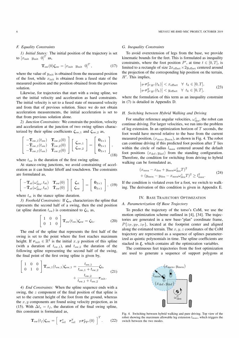
H. Switching between Hybrid Walking and Driving

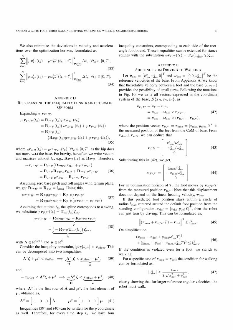
For smaller reference angular velocities, ωzdes, the robot can

continue driving. For larger velocities, we run into the problemof leg extension. In an optimization horizon of T seconds, thefoot would have moved relative to the base from the currentmeasured position, (xmea, ymea), as shown in Fig. 4. The robotcan continue driving if this predicted foot position after T lieswithin the circle of radius lmax centered around the defaultfoot positions (xdef , ydef) from the standing configuration.Therefore, the condition for switching from driving to hybridwalking can be formulated as,

(xmea − xdes + ymeaωzdesT )2

+ (ymea − ydes − xmeaωzdesT )2 ≥ l2max.

(24)

If the condition is violated even for a foot, we switch to walk-ing. The derivation of this condition is given in Appendix E.

IV. BASE TRAJECTORY OPTIMIZATION

A. Parameterization Of Base Trajectory

To predict the trajectory of the torso’s CoM, we use themotion optimization scheme outlined in [4], [34]. The trajec-tories are generated in a new base-"plan" coordinate frame,P{zP , yP , zP}, located at the footprint center and alignedalong the estimated terrain. The x, y, z coordinates of the CoMtrajectory are represented as a sequence of splines parameter-ized as quintic polynomials in time. The spline coefficients arestacked in ξ, which contains all the optimization variables.

The continuous feet trajectories from the foot optimizationare used to generate a sequence of support polygons at

Fig. 4. Switching between hybrid walking and pure driving. Top view of therobot showing the maximum allowable leg extension lmax, which triggers theswitch between the two modes.

SANKAR et al.: TO FOR HYBRID WALKING-DRIVING MOTIONS ON WHEELED QUADRUPEDAL ROBOTS 7

multiple time instants over the optimization horizon. Threesplines are allocated for every consecutive pair of supportpolygons, corresponding to the three DoF of the base we areoptimizing for. Therefore, for np support polygons over thehorizon, we require 3(np − 1) splines. Since each spline has6 polynomial coefficients, the size of ξ is 18(np − 1). If thegait includes full-flight phases, then we reserve two splinesfor each consecutive pair of support polygons and the size ofξ increases accordingly.

B. Objectives

Some of the objectives that contribute to the cost func-tion for the base optimization are similar to that of footoptimization. Over the optimization horizon, we minimizethe acceleration of the base for smooth motions, as in (8)[38]. Moreover, the deviations in positions, velocities andaccelerations between successive optimization solutions areminimized, as in (11).

Additionally, we penalize deviations of the base trajectoryfrom a reference trajectory, or a path regularizer, π(t). Thispath regularizer is obtained as an approximate trajectory forthe base from the external high-level velocities, as in [34].Finally, as a terminal cost, the end of the trajectory is set asa soft constraint to the center of the final support polygon.

The resulting cost function of the base optimization isquadratic in ξ [34].

C. Equality Constraints

The initial states of the trajectory are set as hard constraints,linear in ξ, similar to our approach for foot optimization. Theinitial position and velocity are set to fused states obtainedfrom the current measurements and previous solution, whilethe acceleration is constrained to the state obtained from theprevious solution alone.

For continuity, linear constraints are set for kinematic statesat the junction between splines as in [34]. While the constraintsare set for position and velocity for all junctions, we constrainthe acceleration only if the splines belong to two intersectingsupport polygons.

D. Inequality Constraints

To ensure stability in the sense of balance, we constrainthe zero moment point (ZMP) [39] to lie within the supportpolygon at all time steps in the optimization horizon, T [40].This can be formulated as inequality constraints of the form,[

p q 0]rZMP(tk) + r < 0, ∀tk ∈ [0, T ], (25)

where d = [p q r]T describes the edges of the support polygon

with added safety margins at its boundaries.The position of the ZMP at time t , rZMP(t) ∈ R3, is a

function of the position of CoM, rCoM(t), as,

rx,yZMP(t) =n×

(mrCoM(t)× (g − rCoM(t))− l(t)

)n · (mg −mrCoM(t))

, (26)

where n ∈ R3 is the terrain normal, m ∈ R the mass ofthe base, g ∈ R3 the gravity vector and l ∈ R3 the angular

momentum of the base at the CoM. Since the ZMP positionis nonlinear in the CoM position rCoM(t), it is nonlinear inξ as well. Substituting (26) in (25), the inequality constraints,likewise, are nonlinear in ξ.

If the robot walks on a horizontal flat terrain (n ‖ g) witha constant angular momentum (l = 0) and height of the basefrom the ground (rzCoM = 0), (26) can be simplified greatly toproduce an expression linear in the x, y components of rCoM

as,

rx,yZMP(t) = rx,yCoM(t)− rzCoM(t)

grx,yCoM(t), (27)

where g is the magnitude of the gravitational acceleration. Thisequation can be extended for inclined surfaces by replacingg with the component of gravity along the terrain normaland adding its other components to the accelerations rx,y

respectively.Through these assumptions, we have treated the robot as

a linear inverted pendulum (or a cart-table) model [41], [42].Substituting this in (25), the inequalities become linear in ξ.

In our implementation, the convexity of the base optimiza-tion problem depends on the linearity of the inequality con-straints in ξ. As long as we employ gaits like driving, crawlingor trotting on flat surfaces, the assumptions for the cart-tablemodel are valid. This maintains the base optimization convex,guaranteeing global minima and fast computations.

V. EXPERIMENTAL SETUP AND IMPLEMENTATION

A. Setup

We tested the proposed optimization framework on ANY-mal [4], a quadrupedal robot equipped with nonsteerable,torque-controlled wheels as end-effectors. The robot receivesexternal velocity inputs from a joystick, controlled by the user.The computations were carried out on a PC (Intel i7-7500U,2.7 GHz, dual-core 64-bit) integrated into the robot. Forapplications that require autonomous navigation, the velocitycommands were obtained from a navigation planner, wherethe higher-level computations (such as perception, mapping,localization, path planning, path following, and object detec-tion) were carried out on additional PCs in the robot.

The optimization was implemented in C++ using open-source libraries like Eigen [43] for linear algebraic operationsand QuadProg++ [44] for solving QP based on Goldfarb-Idnani Active-Set algorithm [37]. The base TO uses a customsequential quadratic problem (SQP) algorithm, which solvesthe NLP problem by iterating through a sequence of QPproblems. Rigid Body Dynamics Library, RDBL [45] andKindr [46] were used for kinematics and dynamics, whilesimulating in Gazebo [47] with Open Dynamics Engine, ODE[48] as a physics engine.

For tracking the operational space reference variables, weuse a WBC, inspired from [49], that generates the torquecommands for the joints by solving a sequence of prioritizedconstraints. The WBC is extended for ANYmal on wheels, asdescribed in [4], incorporating the additional rolling constraintassociated with the wheels.

The feet TO, base TO and the WBC run parallel in multiplethreads. The WBC and the state estimation (as established in

8 ME51032 ME-BMD MSC PROJECT, OCTOBER 2019

[49], [50] and extended for ANYmal on wheels as in [4]) runin a fixed 400 Hz loop. The trajectory optimizations, however,are not bound by time. Therefore, the observed frequencies ofthese optimizations reflect their solver times. If either of thefoot or base optimization fails, we use the solution from thecorresponding previously successful optimization.

B. Implementation

As in [26], we set the pitch and roll of the base w.r.t.W-frame to zero at all times. This is crucial for our initialassumption that the heading directions of the base and wheelsare always the same.

The external commands for linear velocity vdes =[vxdes v

ydes 0

]Tand the angular velocity ωdes =

[0 0 ωz

des

]Tof the base are given in the "control" C-frame. Althoughadditional velocity commands, like vzdes and ωxy

des, can pro-vide more functionality to our robot, our options for thesecommands are limited by most off-the-shelf joysticks.

In the foot TO, some objective terms, like (10) and (11), aswell as the inequality constraints in (23), require discretizingthe spline segments in intervals of ∆t. In our implementation,we set an arbitrary lower threshold for ∆t as 2 ms and anupper threshold of ti/50, where ti is the spline duration. Forsplines with durations lower than 2 ms, we skip adding theoptimization variables as well as the corresponding objectiveterms and constraints to our optimization.

The ZMP-based inequality constraints (25) in base TOalso require discretization of the planning horizon. Thesampled time, ∆t, in seconds, was obtained as ∆t =min(0.085,∆tevent), where ∆tevent is the time until the nexttouchdown/liftoff event caused by one or more legs.

C. Analysis

We use the mechanical cost of transport (COTm), a di-mensionless quantity, to compare the energy efficiencies ofdifferent gaits during locomotion. For legged robots, we followthe definition as in [5], where it is the ratio of the power inputsfrom the motors to the power equivalence of the locomotionspeed, given as,

COTm =

1N

N∑k=1

4∑j=1

4∑i=1

max(τijkuijk, 0)

mgvavg, (28)

where τijk is the produced torque and uijk the angular velocityof the joint i of leg j at the time instant k (of a total Nsamples). The variables m, g and vavg denote the mass of thebase, the gravitational acceleration and the average velocity ofthe base in W-frame.

VI. RESULTS AND DISCUSSIONS

A. Gaits

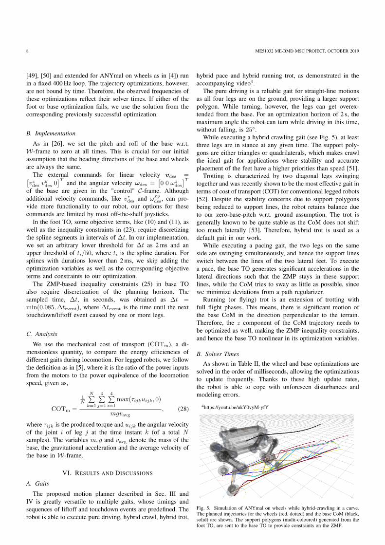
The proposed motion planner described in Sec. III andIV is greatly versatile to multiple gaits, whose timings andsequences of liftoff and touchdown events are predefined. Therobot is able to execute pure driving, hybrid crawl, hybrid trot,

hybrid pace and hybrid running trot, as demonstrated in theaccompanying video4.

The pure driving is a reliable gait for straight-line motionsas all four legs are on the ground, providing a larger supportpolygon. While turning, however, the legs can get overex-tended from the base. For an optimization horizon of 2 s, themaximum angle the robot can turn while driving in this time,without falling, is 25◦.

While executing a hybrid crawling gait (see Fig. 5), at leastthree legs are in stance at any given time. The support poly-gons are either triangles or quadrilaterals, which makes crawlthe ideal gait for applications where stability and accurateplacement of the feet have a higher priorities than speed [51].

Trotting is characterized by two diagonal legs swingingtogether and was recently shown to be the most effective gait interms of cost of transport (COT) for conventional legged robots[52]. Despite the stability concerns due to support polygonsbeing reduced to support lines, the robot retains balance dueto our zero-base-pitch w.r.t. ground assumption. The trot isgenerally known to be quite stable as the CoM does not shifttoo much laterally [53]. Therefore, hybrid trot is used as adefault gait in our work.

While executing a pacing gait, the two legs on the sameside are swinging simultaneously, and hence the support linesswitch between the lines of the two lateral feet. To executea pace, the base TO generates significant accelerations in thelateral directions such that the ZMP stays in these supportlines, while the CoM tries to sway as little as possible, sincewe minimize deviations from a path regularizer.

Running (or flying) trot is an extension of trotting withfull flight phases. This means, there is significant motion ofthe base CoM in the direction perpendicular to the terrain.Therefore, the z component of the CoM trajectory needs tobe optimized as well, making the ZMP inequality constraints,and hence the base TO nonlinear in its optimization variables.

B. Solver Times

As shown in Table II, the wheel and base optimizations aresolved in the order of milliseconds, allowing the optimizationsto update frequently. Thanks to these high update rates,the robot is able to cope with unforeseen disturbances andmodeling errors.

4https://youtu.be/ukY0vyM-yfY

Fig. 5. Simulation of ANYmal on wheels while hybrid-crawling in a curve.The planned trajectories for the wheels (red, dotted) and the base CoM (black,solid) are shown. The support polygons (multi-coloured) generated from thefoot TO, are sent to the base TO to provide constraints on the ZMP.

SANKAR et al.: TO FOR HYBRID WALKING-DRIVING MOTIONS ON WHEELED QUADRUPEDAL ROBOTS 9

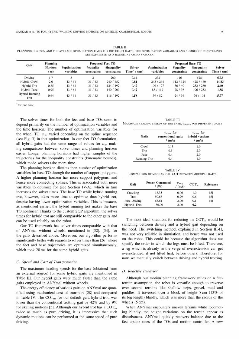
TABLE IIPLANNING HORIZON AND THE AVERAGE OPTIMIZATION TIMES FOR DIFFERENT GAITS. THE OPTIMIZATION VARIABLES AND NUMBER OF CONSTRAINTS

ARE EXPRESSED AS A RANGE, AS <MIN> / <MAX>.

Gait PlanningHorizon

/ (s)

Proposed Feet TO Proposed Base TO#optimization

variables#equality

constraints#inequalityconstraints

SolverTime* / (ms)

#optimizationvariables

#equalityconstraints

#inequalityconstraints

SolverTime / (ms)

Driving 1.7 5 2 200 0.14 232 116 528 6.93Hybrid Crawl 2.0 43 / 61 31 / 43 240 / 452 0.81 243 / 264 112 / 124 428 / 470 14.83Hybrid Trot 0.85 43 / 61 31 / 43 124 / 192 0.47 109 / 127 36 / 40 252 / 280 2.40Hybrid Pace 0.95 43 / 61 31 / 43 140 / 200 0.42 88 / 119 28 / 36 196 / 252 1.88

Hybrid RunningTrot

0.64 43 / 61 31 / 43 116 / 192 0.58 59 / 82 24 / 36 76 / 104 5.77

*for one foot.

The solver times for both the feet and base TOs seem todepend primarily on the number of optimization variables andthe time horizon. The number of optimization variables forthe wheel TO, ns, varied depending on the spline sequence(see Fig. 3) in that optimization. In our feet TO formulation,all hybrid gaits had the same range of values for ns, mak-ing comparisons between solver times and planning horizoneasier. Longer planning horizons had higher samples of thetrajectories for the inequality constraints (kinematic bounds),which made solvers take more time.

The planning horizon dictates then number of optimizationvariables for base TO through the number of support polygons.A higher planning horizon has more support polygons, andhence more connecting splines. This is associated with morevariables to optimize for (see Section IV-A), which in turnincreases the solver times. The base TO while hybrid runningtrot, however, takes more time to optimize than hybrid trot,despite having lower optimization variables. This is because,as mentioned earlier, the hybrid running trot makes the baseTO nonlinear. Thanks to the custom SQP algorithm, the solvertimes for hybrid trot are still comparable to the other gaits andcan be used reliably on the robot.

Our TO framework has solver times comparable with thatof ANYmal without wheels, mentioned in [32], [34], forthe gaits described above. Moreover, our algorithm performssignificantly better with regards to solver times than [26] wherethe feet and base trajectories are optimized simultaneously,which took 20 ms for the same hybrid gaits.

C. Speed and Cost of Transportation

The maximum heading speeds for the base (obtained froman external source) for some hybrid gaits are mentioned inTable III. Our hybrid gaits were much faster than the samegaits employed in ANYmal without wheels.

The energy efficiency of various gaits on ANYmal are quan-tified using mechanical cost of transport (28) and comparedin Table IV. The COTm for our default gait, hybrid trot, waslower than the conventional trotting gait by 42% and by 9%for skating motions [5]. Although our hybrid trot has a COTm

twice as much as pure driving, it is impressive that suchdynamic motions can be performed at the same speed of puredriving.

TABLE IIIMAXIMUM HEADING SPEEDS OF THE BASE, vmax , FOR DIFFERENT GAITS

Gaitsvmax for

conventional gaits/ (m/s)

vmax forhybrid versions

/ (m/s)

Crawl 0.15 1.0Trot 0.5 2.0Pace 0.4 2.0

Running Trot 0.4 1.0

TABLE IVCOMPARISON OF MECHANICAL COT BETWEEN MULTIPLE GAITS

Gait Power Consumed/ (W)

vavg/ (m/s)

COTm Reference

Crawling 18.35 0.06 1.0 [5]Trot 50.68 0.29 0.6 [5]

Pure Driving 63.64 2.00 0.1 [4]Hybrid Trot 156.00 2.00 0.2 -

The most ideal situation, for reducing the COTm would beswitching between driving and a hybrid gait depending onthe need. The switching method, explained in Section III-H,was not very reliable in simulation, and hence was not usedon the robot. This could be because the algorithm does notspecify the order in which the legs must be lifted. Therefore,a leg which is already in the verge of overextension can getoverextended, if not lifted first, before others. Therefore, fornow, we manually switch between driving and hybrid trotting.

D. Reactive Behavior

Although our motion planning framework relies on a flat-terrain assumption, the robot is versatile enough to traverseover several terrains like shallow steps, gravel, mud andpuddles. It traversed over a block of height 8 cm (13% ofits leg length) blindly, which was more than the radius of thewheels (5 cm).

When ANYmal encounters uneven terrains while locomot-ing blindly, the height variations on the terrain appear asdisturbances. ANYmal quickly recovers balance due to thefast update rates of the TOs and motion controller. A new

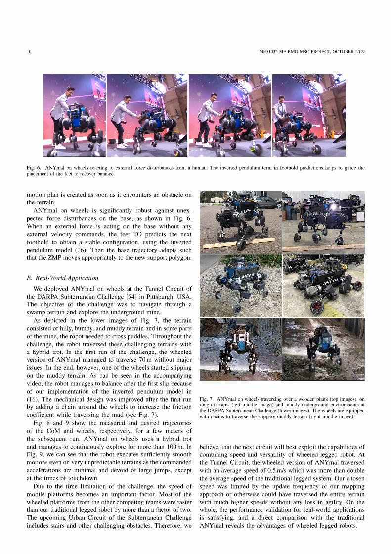
10 ME51032 ME-BMD MSC PROJECT, OCTOBER 2019

Fig. 6. ANYmal on wheels reacting to external force disturbances from a human. The inverted pendulum term in foothold predictions helps to guide theplacement of the feet to recover balance.

motion plan is created as soon as it encounters an obstacle onthe terrain.

ANYmal on wheels is significantly robust against unex-pected force disturbances on the base, as shown in Fig. 6.When an external force is acting on the base without anyexternal velocity commands, the feet TO predicts the nextfoothold to obtain a stable configuration, using the invertedpendulum model (16). Then the base trajectory adapts suchthat the ZMP moves appropriately to the new support polygon.

E. Real-World Application

We deployed ANYmal on wheels at the Tunnel Circuit ofthe DARPA Subterranean Challenge [54] in Pittsburgh, USA.The objective of the challenge was to navigate through aswamp terrain and explore the underground mine.

As depicted in the lower images of Fig. 7, the terrainconsisted of hilly, bumpy, and muddy terrain and in some partsof the mine, the robot needed to cross puddles. Throughout thechallenge, the robot traversed these challenging terrains witha hybrid trot. In the first run of the challenge, the wheeledversion of ANYmal managed to traverse 70 m without majorissues. In the end, however, one of the wheels started slippingon the muddy terrain. As can be seen in the accompanyingvideo, the robot manages to balance after the first slip becauseof our implementation of the inverted pendulum model in(16). The mechanical design was improved after the first runby adding a chain around the wheels to increase the frictioncoefficient while traversing the mud (see Fig. 7).

Fig. 8 and 9 show the measured and desired trajectoriesof the CoM and wheels, respectively, for a few meters ofthe subsequent run. ANYmal on wheels uses a hybrid trotand manages to continuously explore for more than 100 m. InFig. 9, we can see that the robot executes sufficiently smoothmotions even on very unpredictable terrains as the commandedaccelerations are minimal and devoid of large jumps, exceptat the times of touchdown.

Due to the time limitation of the challenge, the speed ofmobile platforms becomes an important factor. Most of thewheeled platforms from the other competing teams were fasterthan our traditional legged robot by more than a factor of two.The upcoming Urban Circuit of the Subterranean Challengeincludes stairs and other challenging obstacles. Therefore, we

Fig. 7. ANYmal on wheels traversing over a wooden plank (top images), onrough terrains (left middle image) and muddy underground environments atthe DARPA Subterranean Challenge (lower images). The wheels are equippedwith chains to traverse the slippery muddy terrain (right middle image).

believe, that the next circuit will best exploit the capabilities ofcombining speed and versatility of wheeled-legged robot. Atthe Tunnel Circuit, the wheeled version of ANYmal traversedwith an average speed of 0.5 m/s which was more than doublethe average speed of the traditional legged system. Our chosenspeed was limited by the update frequency of our mappingapproach or otherwise could have traversed the entire terrainwith much higher speeds without any loss in agility. On thewhole, the performance validation for real-world applicationsis satisfying, and a direct comparison with the traditionalANYmal reveals the advantages of wheeled-legged robots.

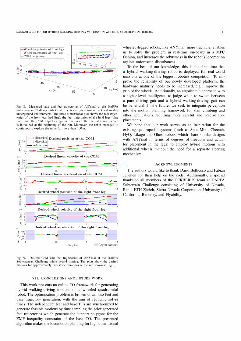
SANKAR et al.: TO FOR HYBRID WALKING-DRIVING MOTIONS ON WHEELED QUADRUPEDAL ROBOTS 11

123

401545

50 1055

5

91.5842.5

2

43 43.5 44 44.5 745

Fig. 8. Measured base and feet trajectories of ANYmal at the DARPASubterranean Challenge. ANYmal executes a hybrid trot on wet and muddyunderground environments. The three-dimensional plot shows the feet trajec-tories of the front legs (red line), the feet trajectories of the hind legs (blueline), and the CoM trajectory (green line) w.r.t. the inertial frame, whichis initialized at the beginning of the run. Moreover, the robot managed tocontinuously explore the mine for more than 100 m.

0 0.5 1 1.50

0.5

0 0.5 1 1.5-0.2

00.20.40.6

0 0.5 1 1.5-202

0 0.5 1 1.50

0.5

0 0.5 1 1.5

-101

0 0.5 1 1.5-200-100

0100

Fig. 9. Desired CoM and feet trajectories of ANYmal at the DARPASubterranean Challenge while hybrid trotting. The plots show the desiredmotions for approximately two stride durations of the run shown in Fig. 8.

VII. CONCLUSIONS AND FUTURE WORK

This work presents an online TO framework for generatinghybrid walking-driving motions on a wheeled quadrupedalrobot. The optimization problem is broken down into feet andbase trajectory generation, with the aim of reducing solvertimes. The independent feet and base TOs are synchronized togenerate feasible motions by time sampling the prior generatedfeet trajectories which generate the support polygons for theZMP inequality constraint of the base TO. The presentedalgorithm makes the locomotion planning for high dimensional

wheeled-legged robots, like ANYmal, more tractable, enablesus to solve the problem in real-time on-board in a MPCfashion, and increases the robustness in the robot’s locomotionagainst unforeseen disturbances.

To the best of our knowledge, this is the first time thata hybrid walking-driving robot is deployed for real-worldmissions at one of the biggest robotics competition. To im-prove the reliability of our newly developed platform, thehardware maturity needs to be increased, e.g., improve thegrip of the wheels. Additionally, an algorithmic approach witha higher-level intelligence to judge when to switch betweena pure driving gait and a hybrid walking-driving gait canbe beneficial. In the future, we seek to integrate perceptioninto the motion planning framework for stair climbing andother applications requiring more careful and precise footplacements.

We hope that our work serves as an inspiration for theexisting quadrupedal systems (such as Spot Mini, Cheetah,HyQ, Likago and Ghost robots, which share similar designswith ANYmal in terms of degrees of freedom and actua-tor placement in the legs) to employ hybrid motions withadditional wheels, without the need for a separate steeringmechanism.

ACKNOWLEDGMENTS

The authors would like to thank Dario Bellicoso and FabianJenelten for their help on the code. Additionally, a specialthanks to all members of the CERBERUS team at DARPASubterrain Challenge consisting of University of Nevada,Reno, ETH Zürich, Sierra Nevada Corporation, University ofCalifornia, Berkeley, and Flyability.

12 ME51032 ME-BMD MSC PROJECT, OCTOBER 2019

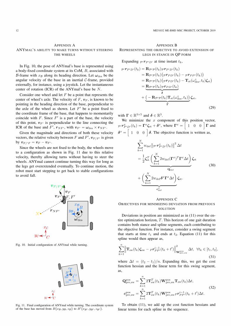
APPENDIX AANYMAL’S ABILITY TO MAKE TURNS WITHOUT STEERING

THE WHEELS

In Fig. 10, the pose of ANYmal’s base is represented usinga body-fixed coordinate system at its CoM, B, associated withB-frame with xB along its heading direction. Let ωdes be theangular velocity of the base in an inertial C-frame, providedexternally, for instance, using a joystick. Let the instantaneouscenter of rotation (ICR) of the ANYmal’s base be N .

Consider one wheel and let F be a point that represents thecenter of wheel’s axle. The velocity of F , vF , is known to bepointing in the heading direction of the base, perpendicular tothe axle of the wheel as shown. Let F ′ be a point fixed tothe coordinate frame of the base, that happens to momentarilycoincide with F . Since F ′ is a part of the base, the velocityof this point, vF ′ is perpendicular to the line connecting theICR of the base and F ′, rNF ′ , with vF ′ = ωdes × rNF ′ .

Given the magnitude and directions of both these velocityvectors, the relative velocity between F and F ′, vF/F ′ is givenby vF/′F = vF − vF ′ .

Since the wheels are not fixed to the body, the wheels moveto a configuration as shown in Fig. 11 due to this relativevelocity, thereby allowing turns without having to steer thewheels. ANYmal cannot continue turning this way for long asthe legs get overextended eventually. To continue motion, therobot must start stepping to get back to stable configurationsto avoid fall.

Fig. 10. Initial configuration of ANYmal while turning.

Fig. 11. Final configuration of ANYmal while turning. The coordinate systemof the base has moved from B{xB, yB, zB} to B′{xB′ , yB′ , zB′}.

APPENDIX BREPRESENTING THE OBJECTIVE TO AVOID EXTENSION OF

LEGS IN STANCE IN QP FORM

Expanding P′rP ′D′ at time instant tk,

P′rP ′D′(tk) = RP′P(tk)PrP ′D′(tk)

= RP′P(tk)(PrPD′(tk)− PrPP ′(tk)

)= RP′P(tk)

(PrPD′(tk)−Tst(ω

zdes, tk)ζst

)= RP′P(tk)PrPD′(tk)︸ ︷︷ ︸

δ

+(−RP′P(tk)Tst(ω

zdes, tk)

)︸ ︷︷ ︸Γ

ζst,

(29)

with Γ ∈ R3×5 and δ ∈ R3.We minimize the x component of this position vector,

P′rxP ′D′(tk) = Γxζst + δx, where Γx =[

1 0 0]

Γ and

δx =[

1 0 0]δ. The objective function is written as,

N∑k=1

wdef

∥∥P′rxP ′D′(tk)∥∥2

∆t

=1

2ζTst

( N∑k=1

2wdef(Γx)TΓx∆t

)︸ ︷︷ ︸

Qdef

ζst

+

( N∑k=1

2wdefδxΓx∆t

)︸ ︷︷ ︸

cTdef

ζst.

(30)

APPENDIX COBJECTIVES FOR MINIMIZING DEVIATION FROM PREVIOUS

SOLUTION

Deviations in position are minimized as in (11) over the en-tire optimization horizon, T . This horizon of one gait durationcontains both stance and spline segments, each contributing tothe objective function. For instance, consider a swing segmentthat starts at time t1 and ends at t2. Equation (11) for thisspline would then appear as,n∑

k=1

∥∥∥Tsw(tk)ζsw − Pri−1PP ′(tk + t′)

∥∥∥2

Wpospre,sw

∆t, ∀tk ∈ [t1, t2],

(31)where ∆t = (t2 − t1)/n. Expanding this, we get the costfunction hessian and the linear term for this swing segment,as,

Qpospre,sw =

n∑k=1

2TTsw(tk)Wpos

pre,swTsw(tk)∆t,

cpospre,sw =

n∑k=1

2TTsw(tk)Wpos

pre,swPri−1PP ′(tk + t′)∆t.

(32)

To obtain (11), we add up the cost function hessians andlinear terms for each spline in the sequence.

SANKAR et al.: TO FOR HYBRID WALKING-DRIVING MOTIONS ON WHEELED QUADRUPEDAL ROBOTS 13

We also minimize the deviations in velocity and accelera-tions over the optimization horizon, formulated as,

N∑k=1

∥∥∥PviP ′(tk)− Pvi−1P ′ (tk + t′)

∥∥∥2

Wvelpre

∆t, ∀tk ∈ [0, T ],

(33)N∑

k=1

∥∥∥PaiP ′(tk)− Pa

i−1P ′ (tk + t′)

∥∥∥2

Waccpre

∆t, ∀tk ∈ [0, T ].

(34)

APPENDIX DREPRESENTING THE INEQUALITY CONSTRAINTS TERM IN

QP FORM

Expanding P′rP ′H′ ,

P′rP ′H′(tk) = RP′P(tk)PrP ′H′(tk)

= RP′P(tk)(PrB′H′(tk) + PrP ′B′(tk)

)= RP′P(tk)(

RPB′(tk)B′rB′H′(tk) + PrP ′B′(tk)),

(35)

where BrBH(tk) = B′rB′H′(tk) ∀tk ∈ [0, T ], as the hip doesnot move w.r.t the base. For brevity, hereafter, we write vectorsand matrices without tk, e.g., RP′P(tk) as RP′P . Therefore,

P′rP ′H′ = RP′P(RPB′BrBH + PrP ′B′

)= RP′PRPB′BrBH + RP′PPrP ′B′

= RP′B′BrBH + RP′PPrP ′B′

(36)

Assuming zero base pitch and roll angles w.r.t. terrain plane,we get RP′B′ = RPB = I3×3. Using this,

P′rP ′H′ = RPBBrBH + RP′PPrP ′B′

= RPBBrBH + RP′P(PrPB′ − PrPP ′

) (37)

Assuming that at time tk, the spline corresponds to a swing,we substitute PrPP ′(tk) = Tsw(tk)ζsw.

P′rP ′H′ = RPBBrBH + RP′PPrPB′︸ ︷︷ ︸µ

+(−RP′PTsw(tk)

)︸ ︷︷ ︸Λ

ζsw,(38)

with Λ ∈ R3×18 and µ ∈ R3.Consider the inequality constraint,

∣∣P′rxP ′H′

∣∣ < xoffset. Thiscan be decomposed into two inequalities:

Λxζ + µx < xoffset =⇒ Λx︸︷︷︸D

ζ < xoffset − µx︸ ︷︷ ︸e

, (39)

and,

− xoffset < Λxζ + µx =⇒ −Λx︸ ︷︷ ︸D

ζ < xoffset + µx︸ ︷︷ ︸e

, (40)

where, Λx is the first row of Λ and µx, the first element ofµ, obtained as,

Λx =[

1 0 0]

Λ, µx =[

1 0 0]µ. (41)

Inequalities (39) and (40) can be written for the y coordinateas well. Therefore, for every time step tk, we have four

inequality constraints, corresponding to each side of the rect-angle foot bound. These inequalities can be extended for stancesplines with the substitution PrPP ′(tk) = Tst(ω

zdes, tk)ζst.

APPENDIX ESHIFTING FROM DRIVING TO WALKING

Let vdes =[vxdes v

ydes 0

]Tand ωdes =

[0 0 ωz

des

]Tbe the

reference velocities of the base. From Appendix A, we knowthat the relative velocity between a foot and the base (vF/F ′)provides the possibility of small turns. Following the notationsin Fig. 10, we write all vectors expressed in the coordinatesystem of the base, B{xB, yB, zB}, as

vF/F ′ = vF − vF ′ ,

= vdes − ωdes × rNF ′ ,

= vdes − ωdes × (rBF ′ − rBN ),

(42)

where the position vector rBF ′ = rmea = [xmea ymea 0]T is

the measured position of the feet from the CoM of base. Fromvdes ⊥ rBN , we can deduce that

rBN =

vydes/ωzdes

−vxdes/ωzdes

0

(43)

Substituting this in (42), we get,

vF/F ′ =

ymeaωzdes

−xmeaωzdes

0

(44)

For an optimization horizon of T , the foot moves by vF/F ′Tfrom the measured position rBF ′ . Note that this displacementdoes not depend on the linear heading velocity, vdes.

If this predicted foot position stays within a circle ofradius lmax centered around the default foot position from thestanding configuration, rdef = [xdef ydef 0]

T , then the robotcan just turn by driving. This can be formulated as,∥∥∥(rmea + vF/F ′T )− rdef

∥∥∥2

≤ l2max. (45)

On simplification,

(xmea − xdef + ymeaωzdesT )2

+ (ymea − ydef − xmeaωzdesT )2 ≤ l2max.

(46)

If the condition is violated even for a foot, we switch towalking.

For a specific case of rmea = rdef , the condition for walkingcan be formulated as,

|ωzdes| ≥

lmax

T√x2

def + y2def

, (47)

clearly showing that for larger reference angular velocities, therobot must walk.

14 ME51032 ME-BMD MSC PROJECT, OCTOBER 2019

REFERENCES

[1] M. Xiangrui, W. Shuo, C. Zhiqiang, and Z. Leijie, “A review ofquadruped robots and environment perception,” 2016 35th ChineseControl Conference (CCC), pp. 6350–6356, 2016.

[2] M. Hutter, R. Diethelm, S. Bachmann, P. Fankhauser, C. Gehring,V. Tsounis, A. Lauber, F. Guenther, M. Bjelonic, L. Isler, H. Kolvenbach,K. Meyer, and M. Hoepflinger, “Towards a generic solution for inspec-tion of industrial sites.” ETH Zurich, 2017-09, 11th Conference onField and Service Robotics (FSR) 2017; Conference Location: Zurich,Switzerland; Conference Date: September 12-15, 2017.

[3] F. Rubio, F. Valero, and C. Llopis-Albert, “A review of mobilerobots: Concepts, methods, theoretical framework, and applications,”International Journal of Advanced Robotic Systems, vol. 16, no. 2, p.172988141983959, 2019. [Online]. Available: http://journals.sagepub.com/doi/10.1177/1729881419839596

[4] M. Bjelonic, D. Bellicoso, Y. De Viragh, D. Sako, F. D. Tresoldi,F. Jenelten, and M. Hutter, “Keep Rollin’-Whole-Body Motion Controland Planning for Wheeled Quadrupedal Robots.” [Online]. Available:https://arxiv.org/pdf/1809.03557.pdf

[5] M. Bjelonic, C. D. Bellicoso, M. E. Tiryaki, and M. Hutter, “Skatingwith a force controlled quadrupedal robot,” 2018, iEEE/RSJ Interna-tional Conference on Intelligent Robots and Systems (IROS 2018);Conference Location: Madrid, Spain; Conference Date: October 1-5,2018; RSL; snf; dfab.

[6] G. Endo and S. Hirose, “Study on roller-walker - energy efficiencyof roller-walk,” 2011 IEEE International Conference on Robotics andAutomation, pp. 5050–5055, 2011.

[7] W. Reid, F. J. Perez-Grau, A. H. Goktogan, and S. Sukkarieh, “Ac-tively articulated suspension for a wheel-on-leg rover operating on aMartian analog surface,” Proceedings - IEEE International Conferenceon Robotics and Automation, vol. 2016-June, pp. 5596–5602, 2016.

[8] K. Iagnemma, A. Rzepniewski, S. Dubowsky, and P. Schenker,“Control of robotic vehicles with actively articulated suspensions inrough terrain,” Autonomous Robots, vol. 14, no. 1, pp. 5–16, Jan 2003.[Online]. Available: https://doi.org/10.1023/A:1020962718637

[9] S. YLÃNEN and A. Halme, “Further development and testing of thehybrid locomotion of workpartner robot,” 01 2002.

[10] M. Takahaashi, K. Yoneda, and S. Hirose, “Rough terrain locomotionof a leg-wheel hybrid quadruped robot,” in Proceedings 2006 IEEEInternational Conference on Robotics and Automation, 2006. ICRA2006., May 2006, pp. 1090–1095.

[11] P. Robuffo Giordano, M. Fuchs, A. Albu-Schäffer, and G. Hirzinger, “Onthe kinematic modeling and control of a mobile platform equipped withsteering wheels and movable legs,” Proceedings - IEEE InternationalConference on Robotics and Automation, pp. 4080–4087, 2009.

[12] A. Dietrich, T. Wimböck, A. Albu-Schäffer, and G. Hirzinger, “Sin-gularity avoidance for nonholonomic, omnidirectional wheeled mobileplatforms with variable footprint,” Proceedings - IEEE InternationalConference on Robotics and Automation, pp. 6136–6142, 2011.

[13] M. Fuchs, C. Borst, P. R. Giordano, A. Baumann, E. Kraemer, J. Lang-wald, R. Gruber, N. Seitz, G. Plank, K. Kunze, R. Burger, F. Schmidt,T. Wimboeck, and G. Hirzinger, “Rollin’ Justin - Design considerationsand realization of a mobile platform for a humanoid upper body,” Pro-ceedings - IEEE International Conference on Robotics and Automation,no. May 2014, pp. 4131–4137, 2009.

[14] F. Cordes, C. Oekermann, A. Babu, D. Kuehn, T. Stark, and F. Kirchner,“An Active Suspension System for a Planetary Rover,” iSAIRAS, no.February 2017, 2014.

[15] M. Giftthaler, F. Farshidian, T. Sandy, L. Stadelmann, and J. Buchli, “Ef-ficient kinematic planning for mobile manipulators with non-holonomicconstraints using optimal control,” Proceedings - IEEE InternationalConference on Robotics and Automation, pp. 3411–3417, 2017.

[16] J. P. Laumond, S. Sekhavat, and F. Lamiraux, Guidelines in nonholo-nomic motion planning for mobile robots, 2006.

[17] M. Wada and H. H. Asada, “Design of a Holonomic OmnidirectionalVehicle Using a Reconfigurable Footprint Mechanism and Its Applica-tion to a Wheelchair.” Journal of the Robotics Society of Japan, vol. 16,no. 6, pp. 816–823, 2012.

[18] A. Suzumura and Y. Fujimoto, “Real-time motion generation and controlsystems for high wheel-legged robot mobility,” IEEE Transactions onIndustrial Electronics, vol. 61, no. 7, pp. 3648–3659, 2014.

[19] C. Grand, F. Benamar, and F. Plumet, “Motion kinematics analysisof wheeledâlegged rover over 3D surface with posture adaptation,”Mechanism and Machine Theory, vol. 45, no. 3, pp. 477–495,2010. [Online]. Available: http://www.sciencedirect.com/science/article/pii/S0094114X09001918

[20] K. K. Hauser, T. Bretl, J.-C. Latombe, and B. Wilcox, “Motion planningfor a six-legged lunar robot,” vol. 47, 01 2006, pp. 301–316.

[21] M. Olinski and J. Ziemba, Hybrid Quadruped Robot â MechanicalDesign and Gait Modelling, 01 2014, vol. 17, pp. 183–190.

[22] T. Klamt, D. Rodriguez, M. Schwarz, C. Lenz, D. Pavlichenko,D. Droeschel, and S. Behnke, “Supervised Autonomous Locomotionand Manipulation for Disaster Response with a Centaur-like Robot,”no. October, 2018. [Online]. Available: http://arxiv.org/abs/1809.06802

[23] A. Laurenzi, E. M. Hoffman, and N. G. Tsagarakis, “Quadrupedalwalking motion and footstep placement through Linear Model PredictiveControl,” pp. 2267–2273, 2018.

[24] T. Klamt and S. Behnke, “Anytime hybrid driving-stepping locomotionplanning,” IEEE International Conference on Intelligent Robots andSystems, vol. 2017-Septe, pp. 4444–4451, 2017.

[25] M. Schwarz, T. Rodehutskors, D. Droeschel, M. Beul, M. Schreiber,N. Araslanov, I. Ivanov, C. Lenz, J. Razlaw, S. Schüller, D. Schwarz,A. Topalidou-Kyniazopoulou, and S. Behnke, “NimbRo Rescue: SolvingDisaster-response Tasks with the Mobile Manipulation Robot Momaro,”Journal of Field Robotics, vol. 34, no. 2, pp. 400–425, 2017.

[26] Y. de Viragh, M. Bjelonic, C. D. Bellicoso, F. Jenelten, and M. Hut-ter, “Trajectory Optimization for Wheeled-Legged Quadrupedal RobotsUsing Linearized ZMP Constraints,” IEEE Robotics and AutomationLetters, vol. 4, no. 2, pp. 1633–1640, 2019.

[27] M. Geilinger, R. Poranne, R. Desai, B. Thomaszewski, and S. Coros,“Skaterbots,” ACM Transactions on Graphics, vol. 37, no. 4, pp. 1–12,2018. [Online]. Available: http://dl.acm.org/citation.cfm?doid=3197517.3201368

[28] B. Dynamics, “Introducing handle,” https://www.youtube.com/watch?v=-7xvqQeoA8c, Feb 2017.

[29] M. Hutter, C. Gehring, D. Jud, A. Lauber, C. D. Bellicoso, V. Tsou-nis, J. Hwangbo, K. Bodie, P. Fankhauser, M. Bloesch, R. Diethelm,S. Bachmann, A. Melzer, and M. Hoepflinger, “Anymal - a highly mo-bile and dynamic quadrupedal robot,” in 2016 IEEE/RSJ InternationalConference on Intelligent Robots and Systems (IROS), Oct 2016, pp.38–44.

[30] A. W. Winkler, C. D. Bellicoso, M. Hutter, and J. Buchli,“Gait and Trajectory Optimization for Legged Systems throughPhase-based End-Effector Parameterization,” IEEE Robotics andAutomation Letters, no. 99, pp. 1–1, 2018. [Online]. Available:http://ieeexplore.ieee.org/document/8283570/

[31] C. Gehring, S. Coros, M. Hutler, C. D. Bellicoso, H. Heijnen, R. Di-ethelm, M. Bloesch, P. Fankhauser, J. Hwangbo, M. Hoepflinger, andR. Siegwart, “Practice makes perfect: An optimization-based approachto controlling agile motions for a quadruped robot,” IEEE RoboticsAutomation Magazine, vol. 23, no. 1, pp. 34–43, March 2016.

[32] C. D. Bellicoso, F. Jenelten, C. Gehring, and M. Hutter, “DynamicLocomotion through Online Nonlinear Motion Optimization forQuadrupedal Robots,” IEEE Robotics and Automation Letters, vol. 3,no. 3, pp. 1–1, 2018. [Online]. Available: http://ieeexplore.ieee.org/document/8260889/

[33] A. W. Winkler, “Optimization-based motion planning for leggedrobots,” p. 100, 2018. [Online]. Available: https://doi.org/10.3929/ethz-b-000272432

[34] C. Dario Bellicoso, F. Jenelten, P. Fankhauser, C. Gehring, J. Hwangbo,and M. Hutter, “Dynamic locomotion and whole-body control forquadrupedal robots,” IEEE International Conference on IntelligentRobots and Systems, vol. 2017-Septe, pp. 3359–3365, 2017.

[35] J. Pratt, J. Carff, S. Drakunov, and A. Goswami, “Capture point: A steptoward humanoid push recovery,” 01 2007, pp. 200 – 207.

[36] M. Raibert, Legged Robots that Balance, ser. Artificial Intelligence.MIT Press, 1986. [Online]. Available: https://books.google.nl/books?id=EXRiBnQ37RwC

[37] D. Goldfarb and A. Idnani, “A numerically stable dual methodfor solving strictly convex quadratic programs,” MathematicalProgramming, vol. 27, no. 1, pp. 1–33, Sep 1983. [Online].Available: https://doi.org/10.1007/BF02591962

[38] M. Kalakrishnan, J. Buchli, P. Pastor, M. Mistry, and S. Schaal, “Learn-ing, planning, and control for quadruped locomotion over challengingterrain,” International Journal of Robotics Research, vol. 30, no. 2, pp.236–258, 2011.

[39] M. Vukobratovic, “Zero-moment pointâproper inter-pretation and new applications,” 2001. [Online].Available: http://www.robot-learning.de/pmwiki/uploads/Research/LocomotionSeminar/vukobratovic_humanoids2001.pdf

[40] P. Sardain and G. Bessonnet, “Forces acting on a biped robot. Center ofpressure-zero moment point,” IEEE Transactions on Systems, Man, and

Cybernetics - Part A: Systems and Humans, vol. 34, no. 5, pp. 630–637,2004.

[41] S. Kajita, F. Kanehiro, K. Kaneko, K. Fujiwara, K. Harada, K. Yokoi,and H. Hirukawa, “Biped Walking Pattern Generation by using PreviewControl of Zero-Moment Point,” Robotics and Automation (ICRA), 2003,pp. 1620–1626, 2003.

[42] A. W. Winkler, F. Farshidian, D. Pardo, M. Neunert, and J. Buchli,“Fast Trajectory Optimization for Legged Robots using Vertex-based ZMP Constraints,” pp. 1–8, 2017. [Online]. Available: http://arxiv.org/abs/1705.10313

[43] G. Guennebaud, B. Jacob et al., “Eigen v3,” http://eigen.tuxfamily.org,2010.

[44] L. D. Gasper, “Quadprog++,” http://quadprog. sourceforge.net.[45] M. L. Felis, “Rbdl: an efficient rigid-body dynamics library using

recursive algorithms,” Autonomous Robots, pp. 1–17, 2016. [Online].Available: http://dx.doi.org/10.1007/s10514-016-9574-0

[46] C. Gehring et al., “Kindr-kinematics and dynamics for robotics,” Nov2018.

[47] O. S. R. Foundation, “Gazebo,” http://gazebosim.org, 2014.[48] S. Russell, “Ode - open dynamics engine,” http://www.ode.org, 2001.

[49] C. Dario Bellicoso, C. Gehring, J. Hwangbo, P. Fankhauser, and M. Hut-ter, “Perception-less terrain adaptation through whole body controland hierarchical optimization,” IEEE-RAS International Conference onHumanoid Robots, pp. 558–564, 2016.

[50] M. Bloesch, M. Burri, H. Sommer, R. Siegwart, and M. Hutter, “TheTwo-State Implicit Filter - Recursive Estimation for Mobile Robots,”IEEE Robotics and Automation Letters, vol. 3, no. 1, pp. 1–1, 2017.[Online]. Available: http://ieeexplore.ieee.org/document/8118116/

[51] P. Fankhauser, M. Bjelonic, D. Bellicoso, T. Miki, and M. Hutter,“Robust Rough-Terrain Locomotion with a Quadrupedal Robot,” Icra,no. May, p. 8, 2018.

[52] H. Kolvenbach, D. Bellicoso, F. Jenelten, L. Wellhausen, and M. Hutter.ESA Conference Bureau, 2018-06-04.

[53] J. Hwangbo, J. Lee, A. Dosovitskiy, D. Bellicoso, V. Tsounis, V. Koltun,and M. Hutter, “Learning agile and dynamic motor skills for leggedrobots,” Science Robotics, vol. 4, no. 26, 2019. [Online]. Available:https://robotics.sciencemag.org/content/4/26/eaau5872

[54] DARPA, “Subterrain challenge,” https://www.subtchallenge.com, 2019.

15