San Jose State University San Jose State University

SJSU ScholarWorks SJSU ScholarWorks

Master's Theses Master's Theses and Graduate Research

Fall 2015

Trajectories of Air Parcel Motions in Mars' Atmosphere Computed Trajectories of Air Parcel Motions in Mars' Atmosphere Computed

Using HYSPLIT Using HYSPLIT

David Bruggeman San Jose State University

Follow this and additional works at: https://scholarworks.sjsu.edu/etd_theses

Recommended Citation Recommended Citation Bruggeman, David, "Trajectories of Air Parcel Motions in Mars' Atmosphere Computed Using HYSPLIT" (2015). Master's Theses. 4625. DOI: https://doi.org/10.31979/etd.9kn2-vwb2 https://scholarworks.sjsu.edu/etd_theses/4625

This Thesis is brought to you for free and open access by the Master's Theses and Graduate Research at SJSU ScholarWorks. It has been accepted for inclusion in Master's Theses by an authorized administrator of SJSU ScholarWorks. For more information, please contact scholarworks@sjsu.edu.

TRAJECTORIES OF AIR PARCEL MOTIONS IN MARS’ ATMOSPHERE

COMPUTED USING HYSPLIT

A Thesis

Presented to

The Faculty of the Department of Meteorology and Climate Science

San José State University

In Partial Fulfillment

of the Requirements for the Degree

Master of Science

by

David Bruggeman

December 2015

© 2015

David Bruggeman

ALL RIGHTS RESERVED

The Designated Thesis Committee Approves the Thesis Titled

TRAJECTORIES OF AIR PARCEL MOTIONS IN MARS’ ATMOSPHERE

COMPUTED USING HYSPLIT

by

David Bruggeman

APPROVED FOR THE DEPARTMENT OF METEOROLOGY AND CLIMATE

SCIENCE

SAN JOSÉ STATE UNIVERSITY

December 2015

Dr. Alison F. C. Bridger Department of Meteorology and Climate Science

Dr. Martin Leach Department of Meteorology and Climate Science

Dr. Melina A. Kahre NASA Ames Research Center

ABSTRACT

TRAJECTORIES OF AIR PARCEL MOTIONS IN MARS’ ATMOSPHERE

COMPUTED USING HYSPLIT

by David Bruggeman

An analysis of the advection of air parcels in the Martian atmosphere during the

2001 global dust storm through the use of three-dimensional trajectories is presented.

The Hybrid Single Particle Lagrangian Integrated Trajectory (HYSPLIT) model, well-

known for trajectory, dispersion, and deposition modeling, and originally developed for

Earth was modified for Mars to provide forward and backward trajectories. The custom

HYSPLIT for Mars uses meteorological input generated by the NASA Ames Mars

General Circulation Model (MGCM). The 2001 global dust storm was the earliest on

record (Ls ~ 180°) and originated from local dust storms around the Hellas basin as the

storm expanded asymmetrically to the east. Trajectories near Hellas and Claritas Fossae

correspond with dust transport detected using satellite imagery. Forward trajectories at Ls

= 184° from Hellas show flow to the south, transporting dust around the south polar cap,

while after Ls = 188° there is an eastward shift in propagation. Air parcel trajectories

intersecting the surface during the dust storm may indicate the processes involved with

global dust storms contributing to dust layers in the polar regions. Backward trajectories

from Claritas Fossae reveal the dust activity in this region was the result of local dust

storm activity instead of the propagation of dust eastward from the Hellas region.

v

ACKNOWLEDGEMENTS

We thank Dr. Roland Draxler of ARL and Dr. Jim Murphy for their valuable help

with HYSPLIT and the MGCM. Thank you to Dr. Housiadas and Dimitris Mitrakos of

the Greek Atomic Energy Commission for their assistance in understanding a way to

modify the conversion program. An extra special thank you to Dr. Bridger for her

patience in the everlasting struggle with HYSPLIT.

vi

TABLE OF CONTENTS

1. Introduction ................................................................................................................... 1

2. Background ................................................................................................................... 6

2.1. Mars .......................................................................................................................... 6

2.2. Atmospheric Structure .............................................................................................. 9

2.3. Hadley Circulation .................................................................................................. 10

2.4. Dust ......................................................................................................................... 12

2.5. Dust Lifting Mechanisms ....................................................................................... 14

2.6. Dust Storms ............................................................................................................ 15

2.7. Polar Layered Deposits ........................................................................................... 18

3. Methods....................................................................................................................... 19

3.1. Overview of HYSPLIT ........................................................................................... 19

3.2. Overview of MGCM .............................................................................................. 23

3.3. Observations ........................................................................................................... 24

3.4. Meteorology File .................................................................................................... 25

3.5. Trajectory Prediction Model ................................................................................... 27

4. 2001 Global Dust Storm ............................................................................................. 30

4.1. Storm Progression................................................................................................... 30

4.2. Claritas Storm Activity ........................................................................................... 34

5. Trajectory Analysis ..................................................................................................... 37

vii

5.1. Hellas ...................................................................................................................... 37

5.2. Claritas .................................................................................................................... 45

6. Discussion and Conclusions ....................................................................................... 50

7. References ................................................................................................................... 54

8. APPENDIX A: Acronyms .......................................................................................... 60

9. APPENDIX B: HYSPLIT Call Chart ......................................................................... 61

viii

LIST OF FIGURES

FIGURE 1: Topographic map of Mars ............................................................................... 4

FIGURE 2: Martian orbital position and seasons ............................................................... 9

FIGURE 3: Conceptual model of Hadley cell circulation ................................................ 12

FIGURE 4: Example trajectories from Fukushima Daiichi accident ............................... 21

FIGURE 5: Flow chart of HYSPLIT process ................................................................... 22

FIGURE 6: MDGM example prior to 2001 global dust storm ......................................... 25

FIGURE 7: MDGM images of Hellas from Ls = 176.12–184.99° ................................... 31

FIGURE 8: MDGM images of south polar cap from Ls = 185.5–191.22° ....................... 33

FIGURE 9: MDGM images of Claritas from Ls = 175.57–196.97° ................................. 36

FIGURE 10: Forward trajectories from western Hellas at Ls = 184° ............................... 40

FIGURE 11: Forward trajectories from central Hellas at Ls = 184°................................. 41

FIGURE 12: Forward trajectories from eastern Hellas at Ls = 184° ................................ 42

FIGURE 13: Forward trajectories from eastern Hellas at Ls = 188° ................................ 43

FIGURE 14: Backward trajectories around south polar cap ............................................ 44

FIGURE 15: Forward trajectories from Claritas at Ls = 188° .......................................... 47

FIGURE 16: Forward trajectories from Claritas at Ls ~ 189.8° ....................................... 48

FIGURE 17: Backward trajectories from Claritas at Ls = 187°........................................ 49

ix

LIST OF TABLES

TABLE 1: Planetary and atmospheric parameters for Earth and Mars .............................. 7

TABLE 2: Observed global dust storms ........................................................................... 17

1

1. Introduction

The determination to learn more about other planets has grown extensively with

the study of our neighbor planet Mars. While the primary focus has been on the past or

future existence of life on Mars, it is not the sole purpose of studying the red planet. The

Mars Atmosphere and Volatile Evolution satellite launched on 18 November 2013 and

reached orbit on 21 September 2014. The satellite collects data on the Martian upper

atmosphere and its interaction with the solar wind. The data allow us to study the history

of the atmosphere and climate (Jakosky et al. 2015). The recognition of another planet’s

environment and climate can help in understanding the complex physics and chemistry

occurring on Earth.

Mars is known for its barren surface and dusty atmosphere. The Martian dust

cycle is a key component of the state of the climate system. For example, dust can

change the albedo of the surface, and interact with the visible and infrared radiation to

alter heating rates in the atmosphere. The dust cloud sizes range from local to global

scales as dust is lifted from the surface and transferred throughout the atmosphere.

Planet-encircling dust storms vary significantly in intensity, when they occur, and in

duration. Dust storms typically occur around the southern hemisphere summer during the

maximum insolation and can distribute dust between both hemispheres as dust can be

lofted several tens of kilometers deep in the atmosphere (Read and Lewis 2004).

An objective of our study is to understand how significant plumes of dust shown

by satellite imagery are transported. This is accomplished by constructing trajectories to

follow dust that is advected around the Martian atmosphere during large dust storms

2

using winds generated from a Mars general circulation model (MGCM). A terrestrial

trajectory prediction model, the Hybrid Single Particle Lagrangian Integrated Trajectory

(HYSPLIT), is used for transport and dispersion modeling based on winds from various

models. HYSPLIT has been modified to allow the input of meteorological data from the

MGCM, a unique application that has not been done prior to this study.

An application of the HYSPLIT presented in this study is to analyze the processes

involved in dust transport for specific regions on Mars during the 2001 global dust storm.

Previous studies observed the initiation and evolution of a global dust storm that occurred

from June to November 2001 using images captured by the Mars Orbiter Camera (MOC)

onboard the Mars Global Surveyor (MGS) satellite. The importance of this global dust

storm is a result of its unusually early occurrence and vast amount of data collected due

to Mars’ favorable orbital position (Strausberg et al. 2005; Cantor 2007). The detailed

observations available from the MGS-MOC are supplemented by the National

Aeronautics and Space Administration (NASA) Ames MGCM to help analyze the source

of the dust storm and the associated atmospheric transport response. Areas of interest

include the Hellas basin impact crater, the source of the global dust storm, and a regional

dust storm in Claritas Fossae that helped sustain high atmospheric dust levels until the

dust filled both hemispheres. Another area includes the south polar cap where alternating

layers of ice and dust known as polar layered deposits (PLDs) have been observed. The

use of backward trajectories from our custom HYSPLIT helps in analyzing how the dust

can settle on the polar surface.

The exploration of Mars began in 1964 where the NASA Mariner 4 captured the

3

first images and temperature of the surface. The USSR successfully landed the Mars 2

spacecraft on the Martian surface in 1969, but the spacecraft failed before it could return

data to Earth. The Viking mission in the summer of 1976 became the first to land on

another planet and return images. The two Viking landers (VLs) touched down on the

northern hemisphere of Mars equipped with 14 instruments designed to analyze the

environment (Read and Lewis 2004). VL-1 landed in western Chryse Planitia and VL-2

in Utopia Planitia (Figure 1). Although the primary objective of the Viking mission was

to identify evidence of living organisms, the VLs were equipped with pressure,

temperature, and wind sensors (Hess et al. 1977). The expected lifespan of the VLs was

90 days; however, VL-1 continued until August 1980 and VL-2 until July 1978. The

meteorology data captured by the VL spacecraft remain invaluable for studies of the

Martian atmosphere (Kieffer et al. 1992; Read and Lewis 2004).

4

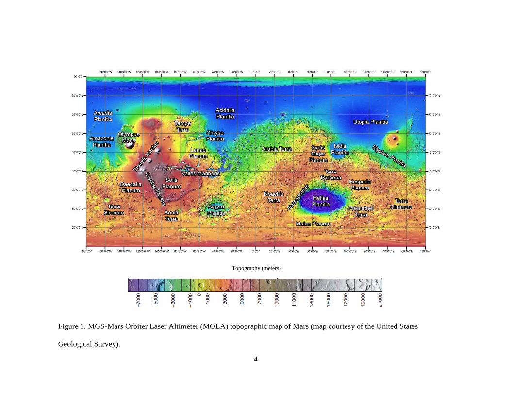
Topography (meters)

Figure 1. MGS-Mars Orbiter Laser Altimeter (MOLA) topographic map of Mars (map courtesy of the United States

Geological Survey).

5

The Mars Pathfinder (MPF), launched by NASA in December 1996 and landed

southeast of VL-1 on 4 July 1997, attempted to demonstrate new lander technology for

future missions. After arrival, MPF served as a scientific mission. MPF obtained an in-

situ atmospheric vertical profile through its entry, and measured surface meteorology

during the nearly 90 days of operation. The images of Mars captured by the VL and MPF

spacecraft revealed a rocky landscape and dusty atmosphere (Magalhães et al. 1999;

Read and Lewis 2004).

A recent spacecraft to orbit Mars and observe atmospheric dust was the MGS

with onboard instruments such as the MOC, Thermal Emission Spectrometer (TES), and

Mars Orbiter Laser Altimeter (MOLA). The MGS began an elliptical orbit around Mars

in September 1997 but transitioned to a nearly circular orbit and to a mapping phase by

March 1999. The MGS was in a polar orbit 12 times per Martian day (sol), collecting

data from 300 km above the surface (Wang and Ingersoll 2002; Read and Lewis 2004).

The MGS-MOC contained a high resolution narrow-angle camera and two low resolution

wide-angle cameras, which were always pointed at the spacecraft’s nadir to provide daily

global surface maps (Cantor et al. 2001). MGS-TES data provide information across the

infrared spectra (~7-50 μm) to determine atmospheric temperature and opacity (Smith et

al. 2002). The MGS-MOLA collected altimetry data to accurately measure the

topography of the planet (Smith et al. 2001). The spacecraft was expected to stop

sending data approximately in April 2003, but continued until November 2006 when the

signal went silent (Wang and Ingersoll 2002; Montabone et al. 2015).

The latest rover sent to Mars is the NASA Mars Science Laboratory (MSL)

6

mission that launched in November 2013 and landed the Curiosity rover in Gale Crater in

August 2012. The radioisotope power system of Curiosity allows for the long-range

mobility (~5–20 km) of the rover for at least one Martian year (MY). The goal of the

mission is to determine the past habitability of the planet (Vasavada et al. 2014).

2. Background

2.1 Mars

Mars was formed ~4.5 × 109 years ago with a counterclockwise orbital and

rotational motion, similar to most of the solar system. Several ancient civilizations

revered Mars and named this red planet appearing in the night sky after a god of war or

death (Read and Lewis 2004). Many planetary features of Mars are similar to Earth,

while atmospheric properties vary greatly (Table 1). A Martian day lasts only 39 minutes

longer than Earth and the axis tilt of both planets is near 24°. Compared with Earth, Mars

is half the size, is 50% farther from the Sun, has a larger orbital eccentricity, has one-

third of the surface gravity, and has a thin atmosphere (1% of Earth) primarily consisting

of carbon dioxide (CO2). Mars’ distinct eccentricity causes 44% more insolation at the

planet’s closest position to the Sun at perihelion compared with aphelion. Other than

Mercury, Mars has the largest eccentricity of the planets in our solar system (Kieffer et

al. 1992; Read and Lewis 2004).

7

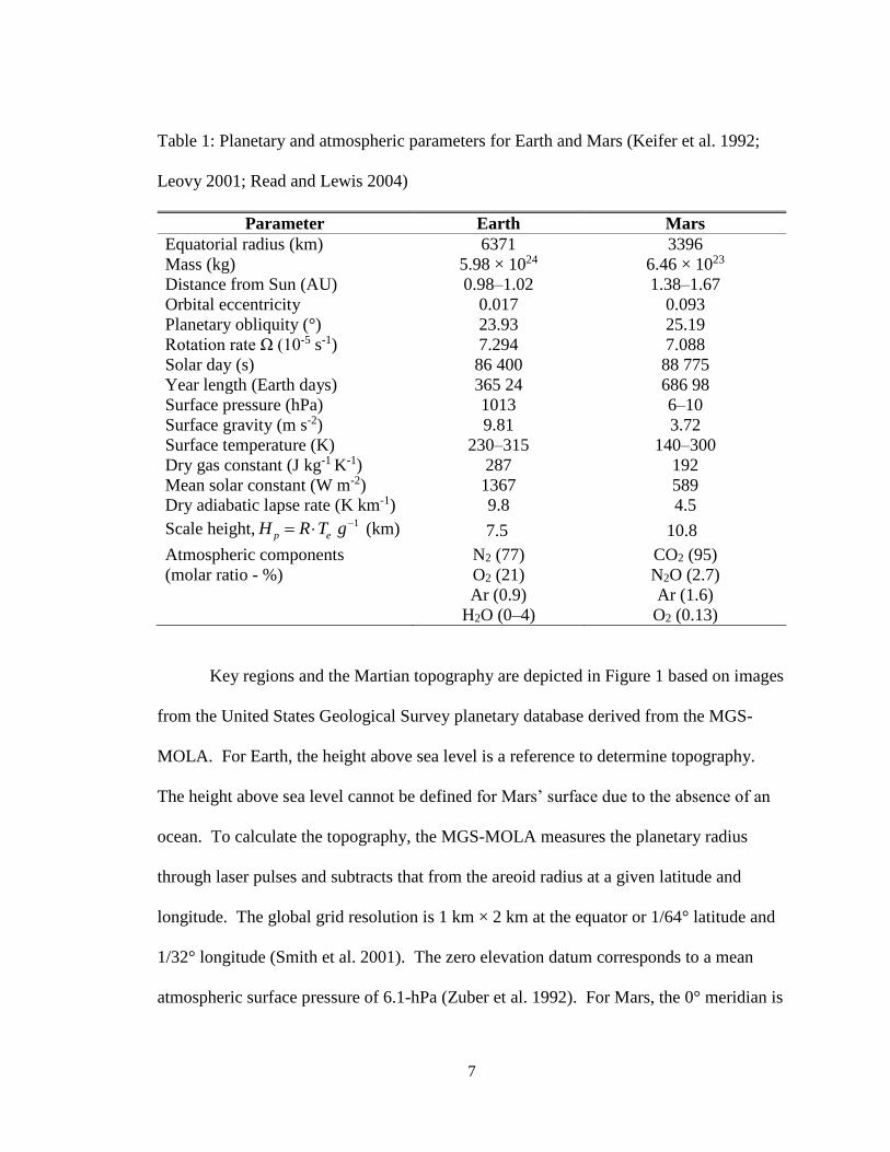
Table 1: Planetary and atmospheric parameters for Earth and Mars (Keifer et al. 1992;

Leovy 2001; Read and Lewis 2004)

Parameter Earth Mars

Equatorial radius (km) 6371 3396

Mass (kg) 5.98 × 1024 6.46 × 1023

Distance from Sun (AU) 0.98–1.02 1.38–1.67

Orbital eccentricity 0.017 0.093

Planetary obliquity (°) 23.93 25.19

Rotation rate Ω (10-5 s-1) 7.294 7.088

Solar day (s) 86 400 88 775

Year length (Earth days) 365 24 686 98

Surface pressure (hPa) 1013 6–10

Surface gravity (m s-2) 9.81 3.72

Surface temperature (K) 230–315 140–300

Dry gas constant (J kg-1 K-1) 287 192

Mean solar constant (W m-2) 1367 589

Dry adiabatic lapse rate (K km-1) 9.8 4.5

Scale height,1

p eH R T g (km) 7.5 8 10.8 8

Atmospheric components N2 (77) CO2 (95)

(molar ratio - %) O2 (21) N2O (2.7)

Ar (0.9) Ar (1.6)

H2O (0–4) O2 (0.13)

Key regions and the Martian topography are depicted in Figure 1 based on images

from the United States Geological Survey planetary database derived from the MGS-

MOLA. For Earth, the height above sea level is a reference to determine topography.

The height above sea level cannot be defined for Mars’ surface due to the absence of an

ocean. To calculate the topography, the MGS-MOLA measures the planetary radius

through laser pulses and subtracts that from the areoid radius at a given latitude and

longitude. The global grid resolution is 1 km × 2 km at the equator or 1/64° latitude and

1/32° longitude (Smith et al. 2001). The zero elevation datum corresponds to a mean

atmospheric surface pressure of 6.1-hPa (Zuber et al. 1992). For Mars, the 0° meridian is

8

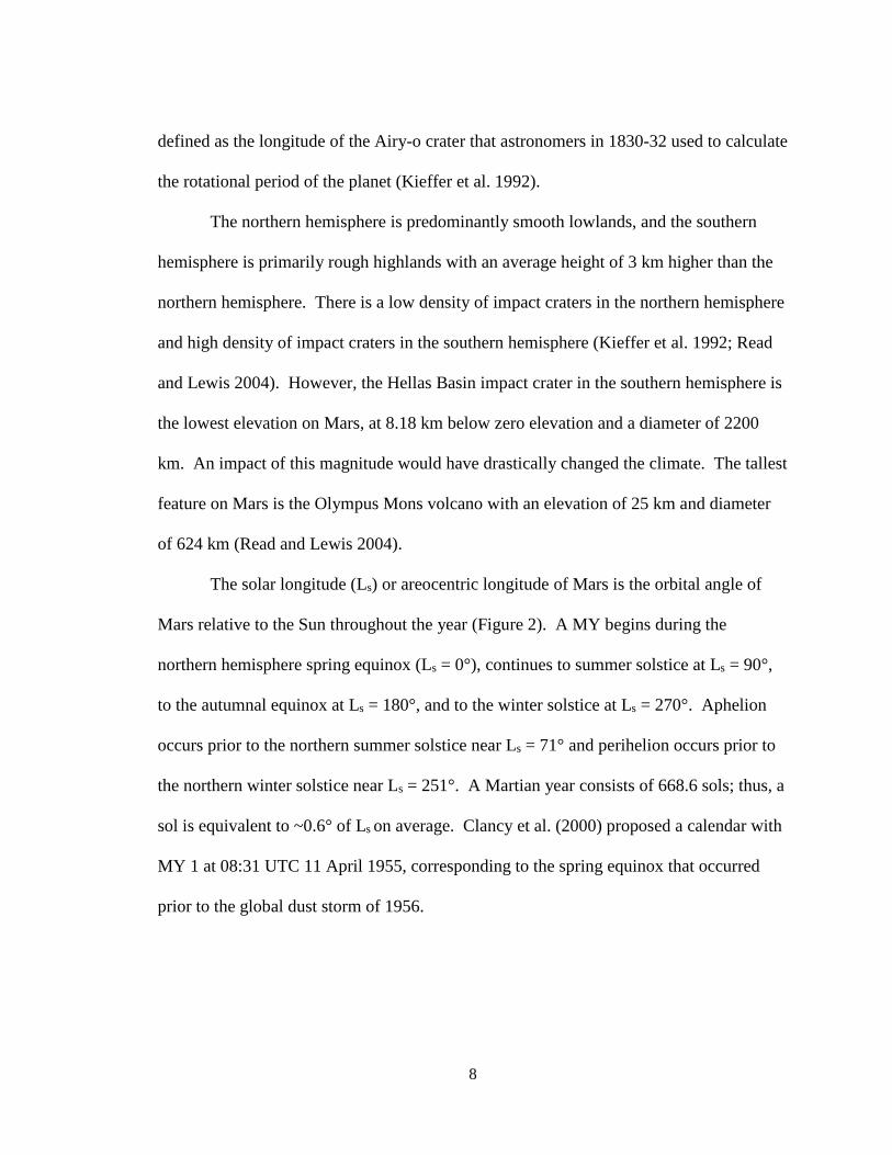
defined as the longitude of the Airy-o crater that astronomers in 1830-32 used to calculate

the rotational period of the planet (Kieffer et al. 1992).

The northern hemisphere is predominantly smooth lowlands, and the southern

hemisphere is primarily rough highlands with an average height of 3 km higher than the

northern hemisphere. There is a low density of impact craters in the northern hemisphere

and high density of impact craters in the southern hemisphere (Kieffer et al. 1992; Read

and Lewis 2004). However, the Hellas Basin impact crater in the southern hemisphere is

the lowest elevation on Mars, at 8.18 km below zero elevation and a diameter of 2200

km. An impact of this magnitude would have drastically changed the climate. The tallest

feature on Mars is the Olympus Mons volcano with an elevation of 25 km and diameter

of 624 km (Read and Lewis 2004).

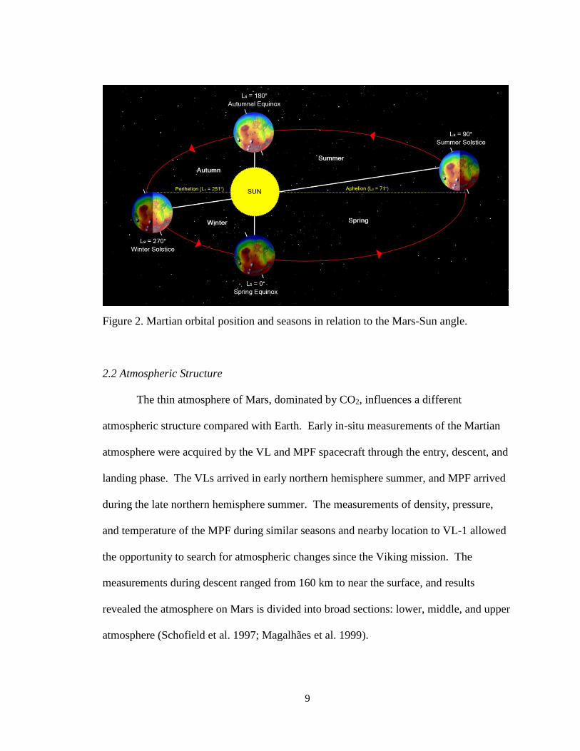
The solar longitude (Ls) or areocentric longitude of Mars is the orbital angle of

Mars relative to the Sun throughout the year (Figure 2). A MY begins during the

northern hemisphere spring equinox (Ls = 0°), continues to summer solstice at Ls = 90°,

to the autumnal equinox at Ls = 180°, and to the winter solstice at Ls = 270°. Aphelion

occurs prior to the northern summer solstice near Ls = 71° and perihelion occurs prior to

the northern winter solstice near Ls = 251°. A Martian year consists of 668.6 sols; thus, a

sol is equivalent to ~0.6° of Ls on average. Clancy et al. (2000) proposed a calendar with

MY 1 at 08:31 UTC 11 April 1955, corresponding to the spring equinox that occurred

prior to the global dust storm of 1956.

9

Figure 2. Martian orbital position and seasons in relation to the Mars-Sun angle.

2.2 Atmospheric Structure

The thin atmosphere of Mars, dominated by CO2, influences a different

atmospheric structure compared with Earth. Early in-situ measurements of the Martian

atmosphere were acquired by the VL and MPF spacecraft through the entry, descent, and

landing phase. The VLs arrived in early northern hemisphere summer, and MPF arrived

during the late northern hemisphere summer. The measurements of density, pressure,

and temperature of the MPF during similar seasons and nearby location to VL-1 allowed

the opportunity to search for atmospheric changes since the Viking mission. The

measurements during descent ranged from 160 km to near the surface, and results

revealed the atmosphere on Mars is divided into broad sections: lower, middle, and upper

atmosphere (Schofield et al. 1997; Magalhães et al. 1999).

10

The lower atmosphere of Mars is comparable to Earth’s stratosphere in regards to

surface pressure and temperature. The surface pressure of Mars ranges from 6–10 hPa

and surface temperatures range from 140–300 K. The variation in surface pressure is the

result of the seasonal variability in CO2 (Leovy 2001; Read and Lewis 2004). Processes

involved in heating the lower atmosphere include the major contributor of the absorption

of sunlight by atmospheric dust and a minor greenhouse effect from CO2 inhibiting

infrared radiation escaping to space. Mars’ thin atmosphere prevents the retention of

daytime heat, creating large temperature fluctuations from day to night (Read and Lewis

2004).

The seasonal and interannual variation in the vertical distribution of dust can

cause an indistinguishable boundary between the lower and middle atmospheres. This

boundary has an average height of ~45 km above ground level (AGL) at a pressure ~0.1-

hPa. The middle atmosphere extends to ~100 km with cold temperatures decreasing with

increasing height. The upper atmosphere extends above 110 km and has an increasing

temperature profile above 120 km where the VL and MPF spacecraft measured a

thermosphere (Schofield et al. 1997; Magalhães et al. 1999; Barlow 2008).

2.3 Hadley Circulation

Previous studies showed a Hadley cell in each hemisphere around equinox (Ls =

180°), similar to Earth, and the development of a single cross-equatorial cell between

30°N and 30°S during the solstices (Haberle et al. 1993). Recent studies with MGCMs

have revealed an asymmetry in the Hadley circulation below 20 km in the annual average

and equinoxes (Takahashi et al. 2003; Zalucha et al. 2010). The asymmetry corresponds

11

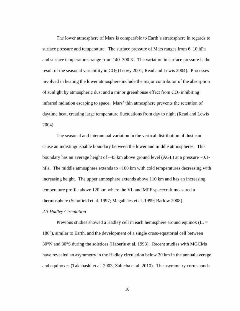
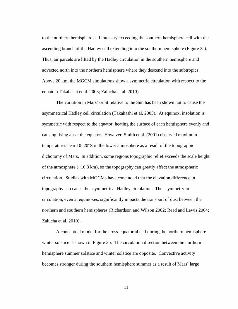
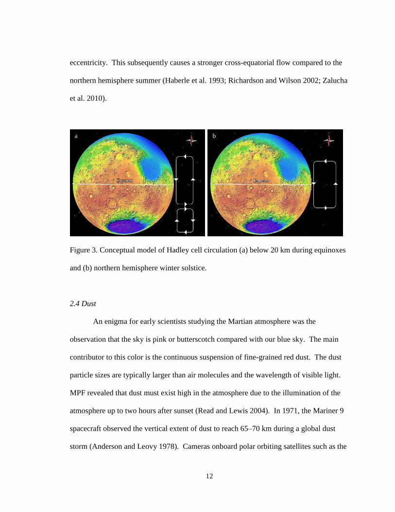
to the northern hemisphere cell intensity exceeding the southern hemisphere cell with the

ascending branch of the Hadley cell extending into the southern hemisphere (Figure 3a).

Thus, air parcels are lifted by the Hadley circulation in the southern hemisphere and

advected north into the northern hemisphere where they descend into the subtropics.

Above 20 km, the MGCM simulations show a symmetric circulation with respect to the

equator (Takahashi et al. 2003; Zalucha et al. 2010).

The variation in Mars’ orbit relative to the Sun has been shown not to cause the

asymmetrical Hadley cell circulation (Takahashi et al. 2003). At equinox, insolation is

symmetric with respect to the equator, heating the surface of each hemisphere evenly and

causing rising air at the equator. However, Smith et al. (2001) observed maximum

temperatures near 10–20°S in the lower atmosphere as a result of the topographic

dichotomy of Mars. In addition, some regions topographic relief exceeds the scale height

of the atmosphere (~10.8 km), so the topography can greatly affect the atmospheric

circulation. Studies with MGCMs have concluded that the elevation difference in

topography can cause the asymmetrical Hadley circulation. The asymmetry in

circulation, even at equinoxes, significantly impacts the transport of dust between the

northern and southern hemispheres (Richardson and Wilson 2002; Read and Lewis 2004;

Zalucha et al. 2010).

A conceptual model for the cross-equatorial cell during the northern hemisphere

winter solstice is shown in Figure 3b. The circulation direction between the northern

hemisphere summer solstice and winter solstice are opposite. Convective activity

becomes stronger during the southern hemisphere summer as a result of Mars’ large

12

eccentricity. This subsequently causes a stronger cross-equatorial flow compared to the

northern hemisphere summer (Haberle et al. 1993; Richardson and Wilson 2002; Zalucha

et al. 2010).

Figure 3. Conceptual model of Hadley cell circulation (a) below 20 km during equinoxes

and (b) northern hemisphere winter solstice.

2.4 Dust

An enigma for early scientists studying the Martian atmosphere was the

observation that the sky is pink or butterscotch compared with our blue sky. The main

contributor to this color is the continuous suspension of fine-grained red dust. The dust

particle sizes are typically larger than air molecules and the wavelength of visible light.

MPF revealed that dust must exist high in the atmosphere due to the illumination of the

atmosphere up to two hours after sunset (Read and Lewis 2004). In 1971, the Mariner 9

spacecraft observed the vertical extent of dust to reach 65–70 km during a global dust

storm (Anderson and Leovy 1978). Cameras onboard polar orbiting satellites such as the

a

b

13

MGS-MOC and the Mars Climate Sounder (MCS) onboard the currently orbiting satellite

Mars Reconnaissance Orbiter (MRO), have also observed this high altitude dust (Read

and Lewis 2004).

Suspended dust provides mid-level atmospheric heating through the absorption of

insolation and infrared radiation. As the suspended dust absorbs insolation, radiation is

prevented from reaching the surface causing cooling near the ground. At night, dust

layers prevent heat from escaping and cause warmer surface temperatures (Read and

Lewis 2004; Barlow 2008).

The column optical depth or optical thickness (τ) is a measure of the fractional

depletion of radiation traveling through an atmospheric column due to absorption and

scattering by dust. During relatively clear days, observations show values of τ in the

range of 0.3–0.5, indicative of a constant background haze of dust. Models show that this

haze can cause global mid-level atmospheric warming at least 5–10 K compared with a

relatively clear atmosphere (Basu et al. 2004). Dust loading increases during southern

hemisphere spring and summer as τ increases to 2–5 and dust loading decreases during

northern hemisphere spring and summer (Read and Lewis 2004).

Montabone et al. (2015) developed the climatology of dust optical depth from

MY 24–31 using measurements from various missions and instruments (e.g., MGS-TES,

MRO-MCS). Results during non-global dust storm years revealed an increase in dust

around Ls = 150° in the southern hemisphere, and a peak between Ls = 210° and 240°.

From Ls = 250–300°, strong dust lifting occurs in the southern polar region. A pause in

large dust storms for other latitudes occurs after Ls ~ 260° as the result of a weakening in

14

low-altitude northern baroclinic waves called the “solstical pause.” After Ls ~ 310°, the

solstical pause ends and a late peak in optical depth occurs (Montabone et al. 2015).

2.5 Dust Lifting Mechanisms

The background haze of dust in the Martian atmosphere is not likely due to slow

dust settlement from global dust storms. Studies show that wind stress and dust devils

contribute to the dust lifting that causes background haze (Basu et al. 2004; Kahre et al.

2006). Kahre et al. (2006) used the MGCM to conclude dust devil lifting contributes to

the background haze during northern hemisphere spring and summer while the annual

opacity maximum during the southern hemisphere spring and summer is the result of

wind stress. Wind stress refers to the lifting of particles as a result of the surface winds.

Sand particles ≥ 20 μm in diameter removed from the surface due to strong low-level

wind stress typically fall immediately to the surface. The process of saltation then takes

place, where particles fall out of the atmosphere, and impact finer particles that become

suspended in the atmosphere. Airborne dust particles typically range from 1–2.5 μm in

diameter (Basu et al. 2004; Read and Lewis 2004).

Dust devils are convective vortices of strong vertical motion and help maintain

the background dust opacity levels. During the summer, thermally-driven convection

during the day can develop a convective boundary layer up to 10 km deep. In areas of

strong heating, the convection can develop a vortex of low pressure and a strong updraft

leading to the formation of a dust devil (Read and Lewis 2004). Dust devils are prevalent

during the southern hemisphere late spring to early fall, and occur more frequently

around Amazonis Planitia (Kahre et al. 2006; Reiss et al. 2014). Dust devils cause dark

15

streaks on the ground as they lift dust from the surface and reveal the dark ground below

(Read and Lewis 2004).

The VL spacecraft first discovered dust devils on Mars and the VLs experienced

the passage of a dust devil over their locations measuring winds greater than 25 m s-1

with gusts up to 44 m s-1 (Ryan and Lucich 1983). The MSL rover Curiosity measured

numerous rapid pressure drops at Gale Crater ranging from 0.5–2.5 Pa, interpreted as dust

devil passage (Kahanpää et al. 2014). Several studies analyzing dust devils using satellite

observations from the MGS, Mars Express (Stanzel et al. 2008), and the MRO (Choi and

Dundas 2011; Reiss et al. 2014) yielded similar results to dust devil wind speed and

direction of motion climatology. Choi and Dundas (2011) calculated tangential speeds

ranging from 20–30 m s-1 and Reiss et al. (2014) found horizontal wind speeds from 4–25

m s-1. The dust devils on Mars are larger in proportion to Earth and can reach several

hundred meters across and have heights of up to 8 km, evidenced through images from

the MGS-MOC (Read and Lewis 2004). Stanzel et al. (2008) found an average height for

dust devils of 660 m and average diameter of 230 m.

2.6 Dust Storms

Dust storms have been observed on Mars in all seasons since the eighteenth

century through the use of telescope and satellite observations (Read and Lewis 2004).

Martian dust storms are categorized based on size and duration as defined by Cantor et al.

(2001). A “local” dust storm has a spatial area limit of 1.6 × 106 km2 or lasts for < 3 sols.

Once a dust storm reaches an area ≥ 1.6 × 106 km2 and lasts > 3 sols, it is called a

“regional” dust storm (Cantor et al. 2001). The dust storm season occurs around

16

perihelion ranging from Ls ~ 161–326°, where regional dust storms are more prevalent to

occur (Martin and Zurek 1993). Local and regional dust storms that occur throughout the

year can significantly elevate dust into the atmosphere. However, the background level

of dust persists in the absence of dust storms (Read and Lewis 2004; Montabone et al.

2015).

A global or planet-encircling dust storm comprises local and regional storms that

yields a sustainable dust cloud with a vertical extent of at least one scale height and

shrouds one or both hemispheres (Cantor et al. 2001). Global dust storms spread dust

over the planet with the convergence of two or more regional storms, and are the rarest

dust storm events occurring every 2–4 MYs (Martin and Zurek 1993). These large dust

storms have been observed primarily in the spring and summer of the southern

hemisphere from Ls = 204–300°, which is the time of maximum insolation (Zurek and

Martin 1993; Montabone et al. 2015). The exception to this time frame is the 2001 global

dust storm that began at Ls ~ 180°.

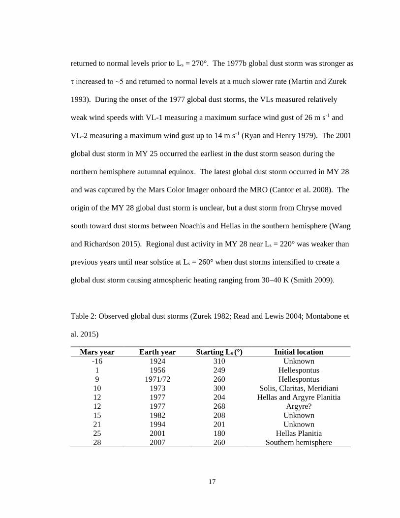
Table 2 shows the global dust storms observed in the past century. Before 2001,

there were five confirmed planet-encircling storms observed in 1956, 1971/72, 1973, and

two in 1977 (Zurek and Martin 1993). The storms listed before 1971 were detected by

telescope observations. The primary locations observed to have initiated previous global

dust storms are around Hellas, the plains near Claritas Fossae, and Isidis Planitia. The

VLs provided visible optical depth and wind speed measurements during two global dust

storms occurring in 1977. Their measurements showed during the first 1977 global dust

storm (1977a), τ increased to ~3 after northern hemisphere autumnal equinox and quickly

17

returned to normal levels prior to Ls = 270°. The 1977b global dust storm was stronger as

τ increased to ~5 and returned to normal levels at a much slower rate (Martin and Zurek

1993). During the onset of the 1977 global dust storms, the VLs measured relatively

weak wind speeds with VL-1 measuring a maximum surface wind gust of 26 m s-1 and

VL-2 measuring a maximum wind gust up to 14 m s-1 (Ryan and Henry 1979). The 2001

global dust storm in MY 25 occurred the earliest in the dust storm season during the

northern hemisphere autumnal equinox. The latest global dust storm occurred in MY 28

and was captured by the Mars Color Imager onboard the MRO (Cantor et al. 2008). The

origin of the MY 28 global dust storm is unclear, but a dust storm from Chryse moved

south toward dust storms between Noachis and Hellas in the southern hemisphere (Wang

and Richardson 2015). Regional dust activity in MY 28 near Ls = 220° was weaker than

previous years until near solstice at Ls = 260° when dust storms intensified to create a

global dust storm causing atmospheric heating ranging from 30–40 K (Smith 2009).

Table 2: Observed global dust storms (Zurek 1982; Read and Lewis 2004; Montabone et

al. 2015)

Mars year Earth year Starting Ls (°) Initial location

-16 1924 310 Unknown

1 1956 249 Hellespontus

9 1971/72 260 Hellespontus

10 1973 300 Solis, Claritas, Meridiani

12 1977 204 Hellas and Argyre Planitia

12 1977 268 Argyre?

15 1982 208 Unknown

21 1994 201 Unknown

25 2001 180 Hellas Planitia

28 2007 260 Southern hemisphere

18

The large quantities of dust lofted by global dust storms has been shown to affect

Hadley cell circulations, atmospheric temperatures, and albedo (Haberle et al. 1993).

MGCM studies have shown that an increase in dust loading at equinox causes a

strengthening in the southern Hadley cell and subsequently shifts the rising branch

northward (Zalucha 2014). Measurements of the 1977a global dust storm by VL-1

yielded a daytime surface temperature decrease of 19 K and nighttime increase of ~15 K

(Ryan and Henry 1979). The change in albedo caused by global dust storms could

influence global surface temperatures as deposition of dust brightens the surface and dust

removal darkens the surface. During the 2001 global dust storm, deposition in the

southern hemisphere increased the albedo by 3.5%, and dust removal in the northern

hemisphere decreased the albedo by 2.5%. The change in albedo potentially caused a

decrease in global average surface temperatures by ~1 K (Cantor 2007).

2.7 Polar Layered Deposits

The polar caps on Mars consist of both a permanent cap that persists all year and a

seasonal CO2 cap that exists from fall through spring. A distinct difference between the

polar caps is that the north residual cap consists of water ice, while the south residual cap

is dominated by CO2 ice with traces of water ice. The north residual cap has a diameter

of 1100 km and covers most of the area poleward of 80°N. By contrast, the south

residual cap extends to 400 km in diameter and is offset from the geographic pole with a

center of 87°S, 315°E (Calvin and Martin 1994; Read and Lewis 2004; Giuranna et al.

2007).

The PLDs exist on the polar caps of Mars and consist of alternating layers of ice

19

and dust that have been observed for decades (Murray et al. 1972; Read and Lewis 2004).

The dust associated with these deposits has been lifted from the surface, transported

through the atmosphere, and deposited in the polar areas. The PLDs stratigraphy are

visible from satellite and are believed to be caused by variations in the Martian climate as

a result of past significant changes in Mars’ obliquity and eccentricity (Read and Lewis

2004; Hvidberg et al. 2012). An objective for this study is to understand the possible

transportation of dust to the polar surface during a global dust storm. HYSPLIT can be

used to produce backward trajectories starting from the polar surface in order to

understand the source of dust that reaches the surface.

3. Methods

3.1 Overview of HYSPLIT

HYSPLIT was developed at the Air Resources Laboratory (ARL) in 1982 through

a collaboration between the National Oceanic and Atmospheric Administration and

Australia’s Bureau of Meteorology. HYSPLIT computes air parcel trajectories,

dispersion, and deposition calculations through a puff or particle approach (Draxler

1999). Initially, the model used only rawinsonde observations as input, but its

capabilities have since expanded (Draxler and Taylor 1982).

HYSPLIT answers the question of how air parcels are transported through the

atmosphere by the advection of winds generated by a wide variety of numerical models.

The model utilizes a hybrid of the Lagrangian approach that moves the frame of reference

with moving air parcels, and the Eulerian approach with a three-dimensional fixed frame

of reference. HYSPLIT includes stability and dispersion equations and advection

20

algorithms to simulate atmospheric transport of single or multiple air parcels. HYSPLIT

version 4.9 has updated the advection algorithm to provide temporal interpolation. The

model is used by a plethora of disciplines ranging from local emergency managers

requesting dispersion forecasts, requests from air quality regulators, and international

dispersion forecasts in case of a large scale nuclear incident (Draxler 1999).

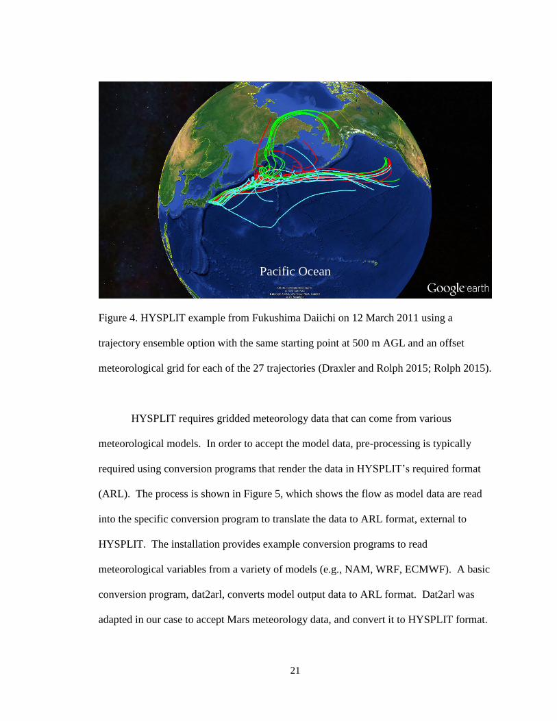
A recent application of HYSPLIT analyzed the Fukushima Daiichi nuclear

complex meltdown in 2011. Figure 4 shows an example of trajectories calculated by

HYSPLIT from the Fukushima site starting at 12 March 2011 from 500 m AGL for a

120-hour duration. This example employs the ensemble option that starts multiple

trajectories from the same point, but offsets the horizontal and vertical meteorological

grid by one grid point in every direction resulting in 27 trajectories. Several studies used

HYSPLIT to analyze the dispersion and transport of radionuclides from Fukushima

(Draxler and Rolph 2012; Draxler et al. 2013; Eslinger et al. 2014).

21

Figure 4. HYSPLIT example from Fukushima Daiichi on 12 March 2011 using a

trajectory ensemble option with the same starting point at 500 m AGL and an offset

meteorological grid for each of the 27 trajectories (Draxler and Rolph 2015; Rolph 2015).

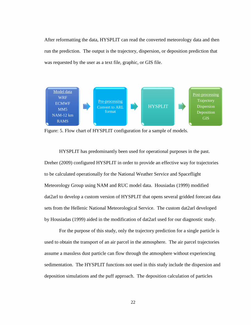
HYSPLIT requires gridded meteorology data that can come from various

meteorological models. In order to accept the model data, pre-processing is typically

required using conversion programs that render the data in HYSPLIT’s required format

(ARL). The process is shown in Figure 5, which shows the flow as model data are read

into the specific conversion program to translate the data to ARL format, external to

HYSPLIT. The installation provides example conversion programs to read

meteorological variables from a variety of models (e.g., NAM, WRF, ECMWF). A basic

conversion program, dat2arl, converts model output data to ARL format. Dat2arl was

adapted in our case to accept Mars meteorology data, and convert it to HYSPLIT format.

Pacific Ocean

22

After reformatting the data, HYSPLIT can read the converted meteorology data and then

run the prediction. The output is the trajectory, dispersion, or deposition prediction that

was requested by the user as a text file, graphic, or GIS file.

Figure: 5. Flow chart of HYSPLIT configuration for a sample of models.

HYSPLIT has predominantly been used for operational purposes in the past.

Dreher (2009) configured HYSPLIT in order to provide an effective way for trajectories

to be calculated operationally for the National Weather Service and Spaceflight

Meteorology Group using NAM and RUC model data. Housiadas (1999) modified

dat2arl to develop a custom version of HYSPLIT that opens several gridded forecast data

sets from the Hellenic National Meteorological Service. The custom dat2arl developed

by Housiadas (1999) aided in the modification of dat2arl used for our diagnostic study.

For the purpose of this study, only the trajectory prediction for a single particle is

used to obtain the transport of an air parcel in the atmosphere. The air parcel trajectories

assume a massless dust particle can flow through the atmosphere without experiencing

sedimentation. The HYSPLIT functions not used in this study include the dispersion and

deposition simulations and the puff approach. The deposition calculation of particles

Model data

WRF

ECMWF

MM5

NAM-12 km

RAMS

Pre-processing

Convert to ARL format

HYSPLIT

Post-processing

Trajectory

Dispersion

Deposition

GIS

23

would allow the input of particle characteristics (e.g., size, density, shape).

The latest version of HYSPLIT is available at http://ready.arl.noaa.gov/index.php.

An installation package of HYSPLIT is available for Windows PC, Mac OS, UNIX or

LINUX (Draxler 1999). The UNIX version allowed the modification of HYSPLIT’s

source code for this study.

3.2 Overview of MGCM

General circulation models simulate the physical processes occurring in the

atmosphere. The atmospheric general circulation of Mars has been successfully modeled

through the interpretation of data obtained by spacecraft missions to Mars. Popular

models include MGCMs developed at NASA Ames Research Center (Leovy and Mintz

1969), the French Laboratoire de Météorologie Dynamique (Hourdin 1992), Oxford

University (Collins and James 1995), and Princeton University (Wilson and Hamilton

1996).

The meteorology data used for this study come from the NASA Ames MGCM.

The MGCM version 1.7.3 is a hydrostatic, finite difference model that simulates the

Martian atmosphere numerically for a desired period using the Arakawa C-Grid. In this

study, a grid spacing of 7.5° latitude, 9° longitude, and 16 vertical sigma levels is used.

This coarse resolution is used to ensure the functionality of the model and HYSPLIT

process, and requires less computing time. The model outputs primary meteorological

variables such as wind, temperature, and pressure at specified time steps. Our scenario

includes a modest dust loading (τ = 0.3) when the atmosphere is relatively clear. The

radiative heating rates from airborne CO2 and dust are calculated in the model. Water

24

and CO2 ice cloud microphysics schemes are not included (Haberle et al. 1993; Kahre

and Haberle 2010).

The physical modeling required for a general circulation model can be difficult

for extraterrestrial planets due to the lack of observations. Other difficulties include a

condensing atmosphere of CO2 to ice at the poles and a strong contrast of the boundary

layer height; tens of meters at night and exceeding 10 km during the day. The Martian

atmosphere can make the MGCM simpler due to its CO2-dominated atmosphere and lack

of oceans. The absorption of infrared radiation occurs from only CO2 and the complex

ocean-atmosphere coupling can be avoided (Read and Lewis 2004).

3.3 Observations

The MGS spacecraft was in orbit during the 2001 global dust storm in MY 25 and

the MGS-MOC recorded many images of the planet before, during, and after the storm.

Mars Daily Global Map (MDGM) images use daily MGS-MOC images to capture

atmospheric phenomena (e.g., dust storms, water-ice clouds) ranging from MY 24–28.

Each map is a composite of 13 consecutive pairs of daytime red and blue MGS-MOC

global strips at 7.5 km pixel-1 or 3.75 km pixel -1 resolution. The MGS-MOC swaths in

the red and blue wavelengths help identify clouds and dust. Most of the images taken

during the global dust storm are presented in 3.75 km pixel-1 resolution. Note the 13

swath pairs were acquired throughout a sol, thus the maps are asynoptic and do not

represent a snapshot in time. The MDGM images presented here are projected as

cylindrical equatorial maps from 60°N to 60°S, as well as south polar stereographic maps

from 45°S to 90°S (Cantor et al. 2001; Wang and Ingersoll 2002).

25

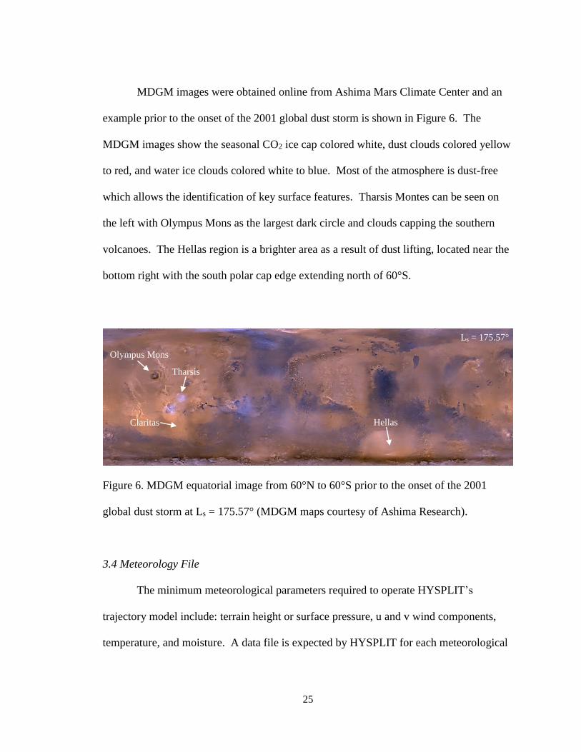
MDGM images were obtained online from Ashima Mars Climate Center and an

example prior to the onset of the 2001 global dust storm is shown in Figure 6. The

MDGM images show the seasonal CO2 ice cap colored white, dust clouds colored yellow

to red, and water ice clouds colored white to blue. Most of the atmosphere is dust-free

which allows the identification of key surface features. Tharsis Montes can be seen on

the left with Olympus Mons as the largest dark circle and clouds capping the southern

volcanoes. The Hellas region is a brighter area as a result of dust lifting, located near the

bottom right with the south polar cap edge extending north of 60°S.

Figure 6. MDGM equatorial image from 60°N to 60°S prior to the onset of the 2001

global dust storm at Ls = 175.57° (MDGM maps courtesy of Ashima Research).

3.4 Meteorology File

The minimum meteorological parameters required to operate HYSPLIT’s

trajectory model include: terrain height or surface pressure, u and v wind components,

temperature, and moisture. A data file is expected by HYSPLIT for each meteorological

Ls = 175.57°

Tharsis

Hellas

Olympus Mons

Claritas

26

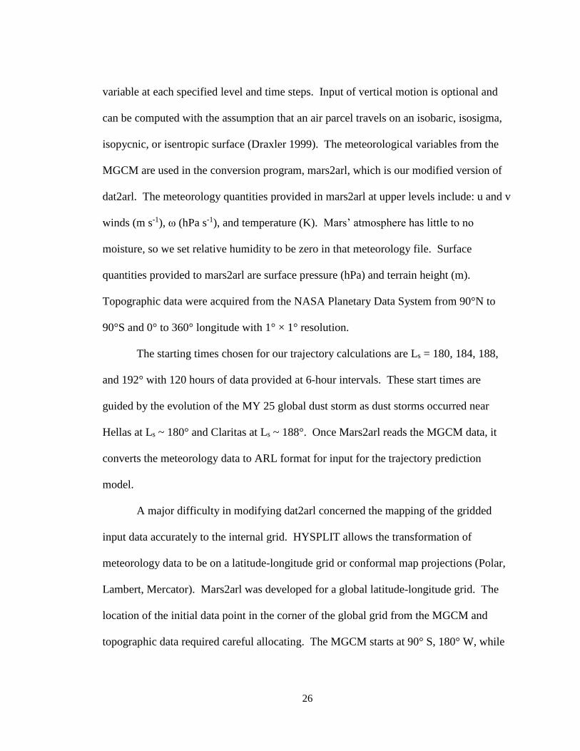
variable at each specified level and time steps. Input of vertical motion is optional and

can be computed with the assumption that an air parcel travels on an isobaric, isosigma,

isopycnic, or isentropic surface (Draxler 1999). The meteorological variables from the

MGCM are used in the conversion program, mars2arl, which is our modified version of

dat2arl. The meteorology quantities provided in mars2arl at upper levels include: u and v

winds (m s-1), ω (hPa s-1), and temperature (K). Mars’ atmosphere has little to no

moisture, so we set relative humidity to be zero in that meteorology file. Surface

quantities provided to mars2arl are surface pressure (hPa) and terrain height (m).

Topographic data were acquired from the NASA Planetary Data System from 90°N to

90°S and 0° to 360° longitude with 1° × 1° resolution.

The starting times chosen for our trajectory calculations are Ls = 180, 184, 188,

and 192° with 120 hours of data provided at 6-hour intervals. These start times are

guided by the evolution of the MY 25 global dust storm as dust storms occurred near

Hellas at Ls ~ 180° and Claritas at Ls ~ 188°. Once Mars2arl reads the MGCM data, it

converts the meteorology data to ARL format for input for the trajectory prediction

model.

A major difficulty in modifying dat2arl concerned the mapping of the gridded

input data accurately to the internal grid. HYSPLIT allows the transformation of

meteorology data to be on a latitude-longitude grid or conformal map projections (Polar,

Lambert, Mercator). Mars2arl was developed for a global latitude-longitude grid. The

location of the initial data point in the corner of the global grid from the MGCM and

topographic data required careful allocating. The MGCM starts at 90° S, 180° W, while

27

the topographic data start at 90° N, 180° W. In addition, the MGCM’s vertical levels

start at the top of the atmosphere, while HYSPLIT expects the first vertical level to be

near the surface. FORTRAN code was written to make the necessary transformations.

3.5 Trajectory Prediction Model

Hymodelt is the main trajectory executable FORTRAN file that calls several

subroutines based on the input meteorology file. There is no published chart that

describes the order in which these subroutines are called by hymodelt. Appendix B was

developed to understand the purpose for each process (blue outline), which files are used

to calculate trajectory predications including a description (orange outline), and in what

order they are called. For example, the first step includes determining the starting time

and number of locations. Hymodelt then calls four files including the file, datset, to set

up the date, time, and number of locations. Datset then calls decodi to decode integer

input variables. Because of its original development for Earth, planetary and atmospheric

constants coded in HYSPLIT required modifying in order to convert the model to Mars

(e.g., planetary radius, surface gravity, surface pressure). An investigation of the 50

subroutines in Appendix B ensured a complete transformation to Mars. Some parameters

cause no change in the results due to their primary use in the dispersion and concentration

simulations of HYSPLIT.

As the model reads the horizontal meteorological data fields in mars2arl, an

interpolation of the data to a terrain-following vertical coordinate system ensures an air

parcel flows around the topography. The meteorological data are allowed to be input on

vertical coordinate systems including pressure-sigma, pressure-absolute, terrain-sigma, or

28

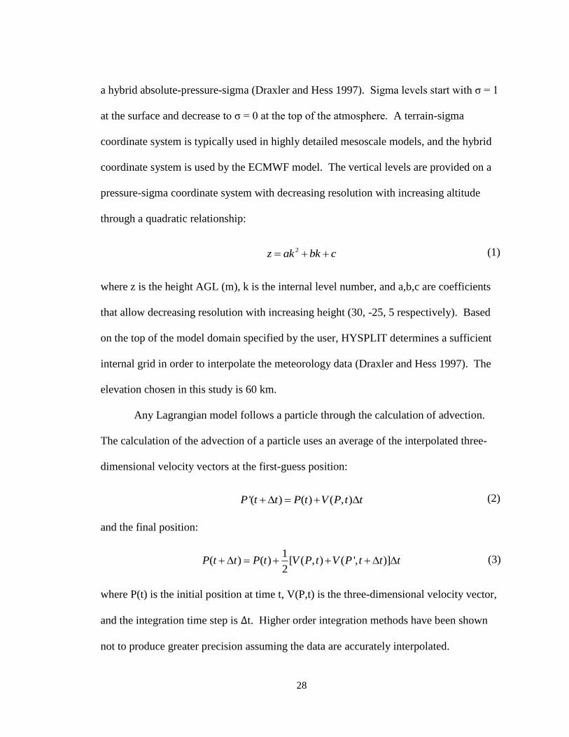
a hybrid absolute-pressure-sigma (Draxler and Hess 1997). Sigma levels start with σ = 1

at the surface and decrease to σ = 0 at the top of the atmosphere. A terrain-sigma

coordinate system is typically used in highly detailed mesoscale models, and the hybrid

coordinate system is used by the ECMWF model. The vertical levels are provided on a

pressure-sigma coordinate system with decreasing resolution with increasing altitude

through a quadratic relationship:

2z ak bk c

where z is the height AGL (m), k is the internal level number, and a,b,c are coefficients

that allow decreasing resolution with increasing height (30, -25, 5 respectively). Based

on the top of the model domain specified by the user, HYSPLIT determines a sufficient

internal grid in order to interpolate the meteorology data (Draxler and Hess 1997). The

elevation chosen in this study is 60 km.

Any Lagrangian model follows a particle through the calculation of advection.

The calculation of the advection of a particle uses an average of the interpolated three-

dimensional velocity vectors at the first-guess position:

'( ) ( ) ( , )P t t P t V P t t

and the final position:

1( ) ( ) [ ( , ) ( ', )]

2P t t P t V P t V P t t t

where P(t) is the initial position at time t, V(P,t) is the three-dimensional velocity vector,

and the integration time step is ∆t. Higher order integration methods have been shown

not to produce greater precision assuming the data are accurately interpolated.

(2)

(3)

(1)

29

Trajectories are stopped when a parcel’s elevation exceeds the top of the model domain.

However, HYSPLIT allows trajectories that intersect the ground to continue to advect on

the surface (Draxler and Hess 1997). For parcels that intersect the ground in this study,

the remaining trajectory is terminated since dust would most likely settle in this area.

During model execution, various constants not associated with the meteorology

file, such as roughness length and land use, were provided to ensure complete

modification of the model to Mars. HYSPLIT utilizes a roughness length to calculate the

horizontal mean wind speed near the surface. The default roughness length file was

replaced with a constant value of 0.01 m based on VL measurements (Sutton et al. 1978).

The purpose of land use is for resuspension calculations and a default land use file for

Earth is provided, but the user can select a specific land use from 11 categories (e.g.,

urban, mixed forest, water) at every grid point. Mars’ complex terrain lacks any water or

vegetation resulting in a rocky land use characteristic for this study.

Various sources can lead to errors in HYSPLIT’s trajectory prediction. A major

component of error can arise from the inaccuracy of the model meteorological fields to

represent the atmosphere, these are called resolution errors. They can occur during

interpolation of meteorological gridded parameters regardless of a high resolution model.

Resolution errors are difficult to quantify independently. However, multiple meteorology

sources can verify an error. Integration errors involve the integration time step in

HYSPLIT and can be minimized with a smaller Δt value. An integration error can be

estimated by executing a forward trajectory and then running a backward trajectory from

the forward trajectory termination (Draxler and Rolph 2007).

30

4. 2001 Global Dust Storm

4.1 Storm Progression

MGS-MOC observations captured the development and decay of a global dust

storm that lasted from June to November 2001 in MY 25 and occurred near Ls = 180°,

southern hemisphere spring. This storm was the earliest and most thoroughly recorded

global dust storm to date (Strausberg et al. 2005; Cantor 2007). During MY 25, detailed

observations were made of Mars’ atmosphere as Earth was positioned directly between

the Sun and Mars. This alignment is referred to as opposition. Opposition occurs for

Earth and Mars every 779 Earth days and the closest proximity occurs when Mars is at

perihelion during opposition, which occurs every 15–17 years (Read and Lewis 2004).

Strausberg et al. (2005) observed the evolution of this storm using MGS-MOC

and MGS-TES data. Cantor (2007) used MGS-MOC images for this storm to conclude

that the storm was initiated by local dust storm activity occurring in seven pulses around

the Hellas region. Six transient baroclinic eddies are believed to have initiated these

precursor storms, causing significant dust lifting (Noble 2013). The storm was then

sustained through several local and regional storms (Strausberg et al. 2005; Cantor 2007).

Figure 7 shows local dust storms around Hellas, at its center, expanding from the

basin prior to the global dust storm. The local storms located around Hellas and Malea

Planum occurred from Ls = 176.2–184.6° (Figures 7a-d) as they spread northward and

eastward at 1.5–16.2 m s-1 (Cantor 2007). After Ls = 184.7°, the dust storm rapidly

expanded asymmetrically to the east from the Hellas region at speeds ranging from 4–32

m s-1 reaching Noachis, Arabia, Syrtis, Tyrrhena, Hesperia, Cimmera, and Malea. Note

31

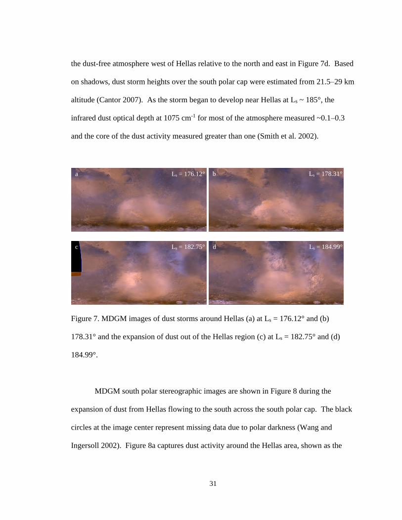
the dust-free atmosphere west of Hellas relative to the north and east in Figure 7d. Based

on shadows, dust storm heights over the south polar cap were estimated from 21.5–29 km

altitude (Cantor 2007). As the storm began to develop near Hellas at Ls ~ 185°, the

infrared dust optical depth at 1075 cm-1 for most of the atmosphere measured ~0.1–0.3

and the core of the dust activity measured greater than one (Smith et al. 2002).

Figure 7. MDGM images of dust storms around Hellas (a) at Ls = 176.12° and (b)

178.31° and the expansion of dust out of the Hellas region (c) at Ls = 182.75° and (d)

184.99°.

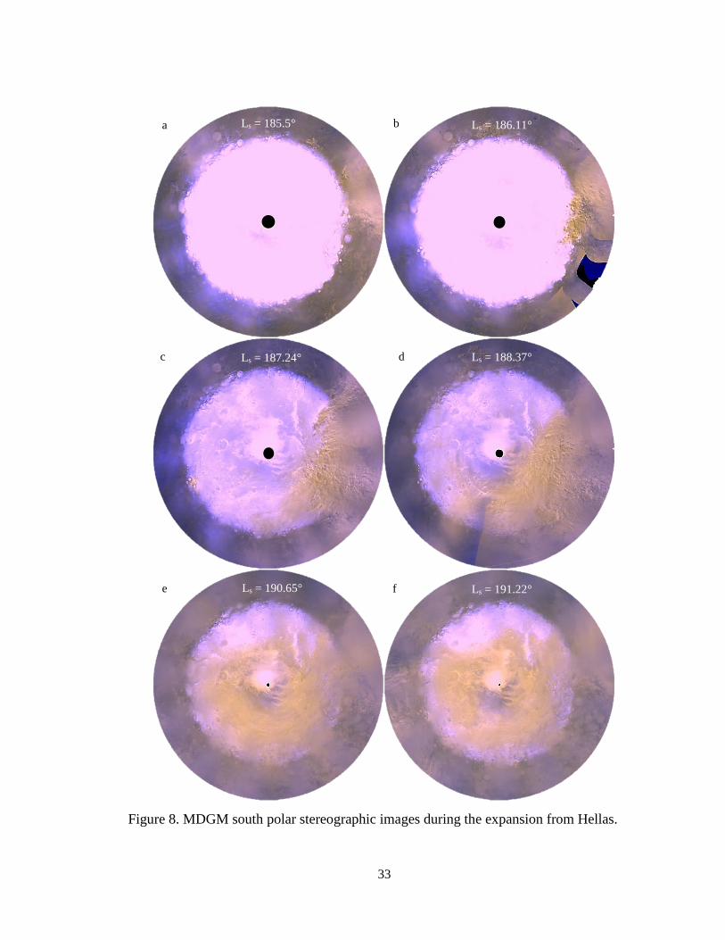
MDGM south polar stereographic images are shown in Figure 8 during the

expansion of dust from Hellas flowing to the south across the south polar cap. The black

circles at the image center represent missing data due to polar darkness (Wang and

Ingersoll 2002). Figure 8a captures dust activity around the Hellas area, shown as the

a Ls = 176.12°

b Ls = 178.31°

c Ls = 182.75°

d Ls = 184.99°

32

bright region on the right, revealing only the southern half of Hellas. At this time, the

south polar cap is dust-free with evidence of water ice clouds around the perimeter of the

cap edge. The dust originating from Hellas travels to the south over the polar region by

Ls ~ 186° (Figure 8b). After this time, dust is wrapping clockwise around the cap and

begins to obscure the polar cap surface (Figures 8c, 8d). By Ls = 190.65° (Figure 8e), the

dust injection from Hellas toward the south pole decreases as evidenced by the nearly

entire cap edge that can be seen through the dust haze. After Ls = 191.22° (Figure 8f),

the flow of dust is significantly cut-off from Hellas and a dust haze remains in this area

throughout the duration of the global dust storm.

33

Figure 8. MDGM south polar stereographic images during the expansion from Hellas.

Ls = 187.24°

e

f

Ls = 188.37°

Ls = 185.5°

Ls = 186.11°

Ls = 190.65°

Ls = 191.22°

a

b

c

d

34

The Hellas storm activity became planet-encircling in the southern hemisphere

by Ls = 192.3° and expanded into the northern hemisphere. The dust shroud obscured the

surface between 60°N and 59°S by Ls = 197.0° except for the 20+ km high volcanoes in

the northern hemisphere. Even though regional storms around the Hellas and Claritas

regions continued at Ls = 200.4°, the optical depth began to diminish as dust settled to the

surface. The primary dust clearing occurred until Ls = 263.4° while the dust opacity took

until Ls = 304° to reach a seasonal low (Strausberg et al. 2005; Cantor 2007).

The main direction of propagation for the 2001 global dust storm differed from

prior global dust storms. The 2001 storm propagated to the east while previous storms

were observed to propagate to the west. Cantor (2007) estimated the general circulation

of the atmosphere between Ls = 175–199° in MY 25 to be to the east with wind speeds

ranging from 3–32 m s-1. The dust opacity around Hellas rapidly increased from τ ~ 1 at

Ls = 184.5° to a peak at Ls = 199.5° of τ ~ 5.0 (Cantor 2007).

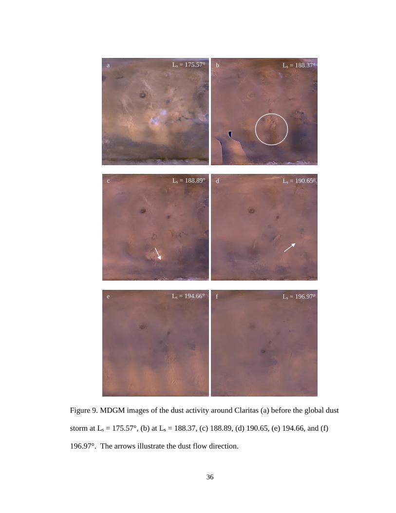
4.2 Claritas Storm Activity

The Hellas storm activity was not the sole contributor to the MY 25 planet-

encircling storm. The Claritas Fossae region, south of Tharsis, revealed dust activity at

Ls = 188.2° as shown in Figure 9. Figure 9a shows the Claritas area during the relatively

clear atmosphere before the global dust storm. At Ls = 188.37° (Figure 9b), a significant

plume of dust was located around Claritas, noted with the white circle. The storm

expanded south and east into Solis Planum by Ls = 188.8° (Figure 9c). The Claritas dust

storm became a regional storm on Ls = 189.6° extending from Daedalia Planum to Valles

Marineris and south to Aonia Terra. After Ls = 190.5° (Figure 9d), the Claritas regional

35

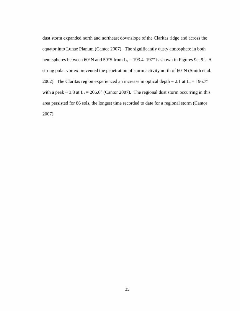
dust storm expanded north and northeast downslope of the Claritas ridge and across the

equator into Lunae Planum (Cantor 2007). The significantly dusty atmosphere in both

hemispheres between 60°N and 59°S from Ls = 193.4–197° is shown in Figures 9e, 9f. A

strong polar vortex prevented the penetration of storm activity north of 60°N (Smith et al.

2002). The Claritas region experienced an increase in optical depth ~ 2.1 at Ls = 196.7°

with a peak ~ 3.8 at Ls = 206.6° (Cantor 2007). The regional dust storm occurring in this

area persisted for 86 sols, the longest time recorded to date for a regional storm (Cantor

2007).

36

Figure 9. MDGM images of the dust activity around Claritas (a) before the global dust

storm at Ls = 175.57°, (b) at Ls = 188.37, (c) 188.89, (d) 190.65, (e) 194.66, and (f)

196.97°. The arrows illustrate the dust flow direction.

a Ls = 175.57° b Ls = 188.37°

Ls = 188.89° Ls = 190.65°

Ls = 194.66° e

d c

Ls = 196.97° f

37

The general circulation patterns for northern hemisphere fall correspond to dust

transport shown by the MDGM images during the 2001 global dust storm. MGCM

studies during equinox show relatively weak mid-latitude westerlies compared with at

solstice, and easterlies near the equator (Haberle et al. 1993). Fenton and Richardson

(2001) used MGCM simulations to calculate seasonal average surface winds. During

northern hemisphere summer (Ls = 90–180°), winds southeast of Hellas flow toward the

south polar cap. Surface winds during northern hemisphere fall (Ls = 180–270°) indicate

clockwise circulation around Hellas, and the flow around Tharsis is to the south as a

result of the topography (Fenton and Richardson 2001).

5. Trajectory Analysis

5.1 Hellas

A matrix of numerous trajectories throughout Hellas and at several vertical levels

was calculated to aid in examining the dust transport from Hellas. Three-dimensional

forward trajectories starting on the perimeter and within the Hellas impact crater are

shown in Figures 10–13. For brevity, the trajectories shown provide a representative

sample for the area. The MGS-MOC topography image is a south polar stereographic

projection with the same topography scale as Figure 1. Based on MDGM images during

the onset of the global dust storm, the south polar cap edge has little variation, with an

estimated extent to ~55°S noted by the dashed line. Figures 10–12 represent trajectories

of air parcels lifted to or released at 500 m, 1.5 km, and 3 km AGL starting at Ls = 184°,

corresponding to the initial expansion of dust out of the Hellas region. Air parcel

trajectories representing dust transport through the atmosphere assume dust loading

38

occurred in that region. Each colored sphere in the figures represents 24 hour increments

or ~0.6° of Ls. The graph below the following figures shows the altitude of each parcel

over 120 hours or ~3° of Ls.

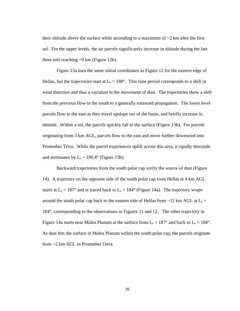
For parcels released from the western edge of Hellas, the lower level trajectories

flow to the north and west and descend to the surface within 24 hours (Figures 10a, 10b).

Parcels released at 3 km move north and east around Hellas, executing clockwise diurnal

motions, and they remain aloft over the elevated terrain east of Hellas by Ls = 187°.

Parcels released above this altitude follow a similar path. During the first 24 hours, as the

parcels move from a higher elevation at the start to a lower elevation into Hellas, the

parcels descend following the terrain (Figure 10b).

Figure 11 is similar to Figure 10 except the starting location is near the center of

Hellas. The air parcels are immediately lofted as much as 3 km above their initial

altitude and remain aloft as they travel south from all levels (Figures 11a, 11b). For

parcels at 500 m, lighter winds near the surface compared with winds aloft cause the

parcel to travel a shorter distance and reach Malea Planum by Ls = 187°. Dust that is

lifted to higher altitudes approaches the cap edge by Ls ~ 185.2° and then continues to

flow clockwise around the south polar cap. The parcels remain suspended and slowly

increase in altitude until reaching near Aonia Terra by Ls = 187°.

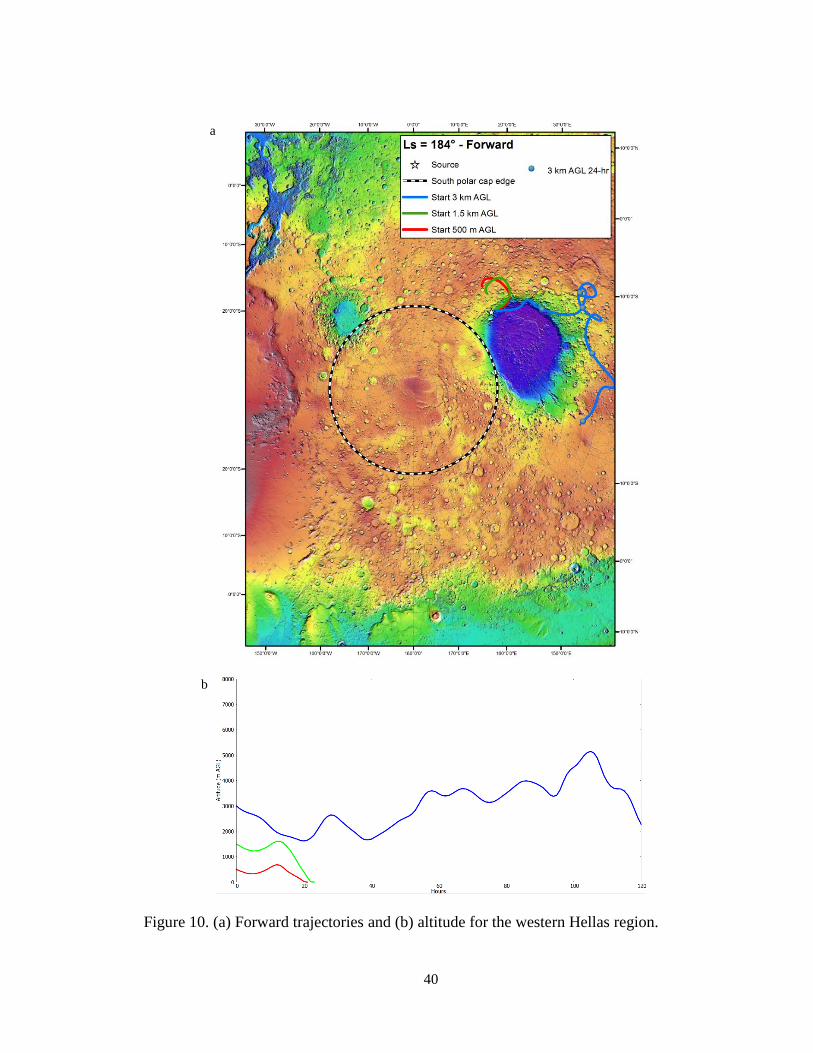
The trajectories originating from the eastern edge of Hellas are shown in Figure

12a. The trajectories follow a similar path to the trajectories released from the center of

Hellas (Figure 11a); the air parcels travel south around the south polar cap ending

southwest of Argyre Planitia by Ls = 187°. Parcels starting at 500 m generally maintain

39

their altitude above the surface while ascending to a maximum of ~2 km after the first

sol. For the upper levels, the air parcels significantly increase in altitude during the last

three sols reaching ~9 km (Figure 12b).

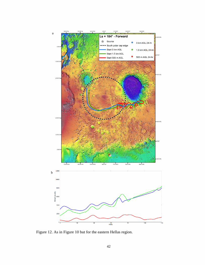
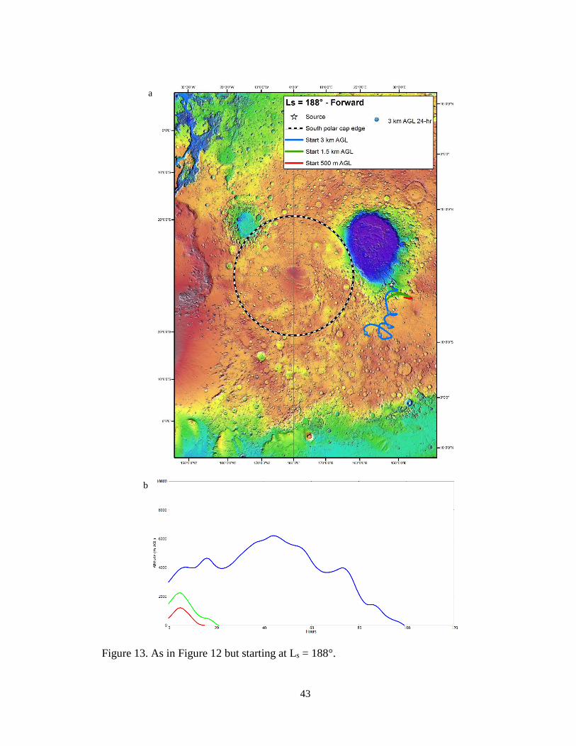
Figure 13a uses the same initial coordinates as Figure 12 for the eastern edge of

Hellas, but the trajectories start at Ls = 188°. This time period corresponds to a shift in

wind direction and thus a variation in the movement of dust. The trajectories show a shift

from the previous flow to the south to a generally eastward propagation. The lower level

parcels flow to the east as they travel upslope out of the basin, and briefly increase in

altitude. Within a sol, the parcels quickly fall to the surface (Figure 13b). For parcels

originating from 3 km AGL, parcels flow to the east and move further downwind into

Promethei Terra. While the parcel experiences uplift across this area, it rapidly descends

and terminates by Ls ~ 190.4° (Figure 13b).

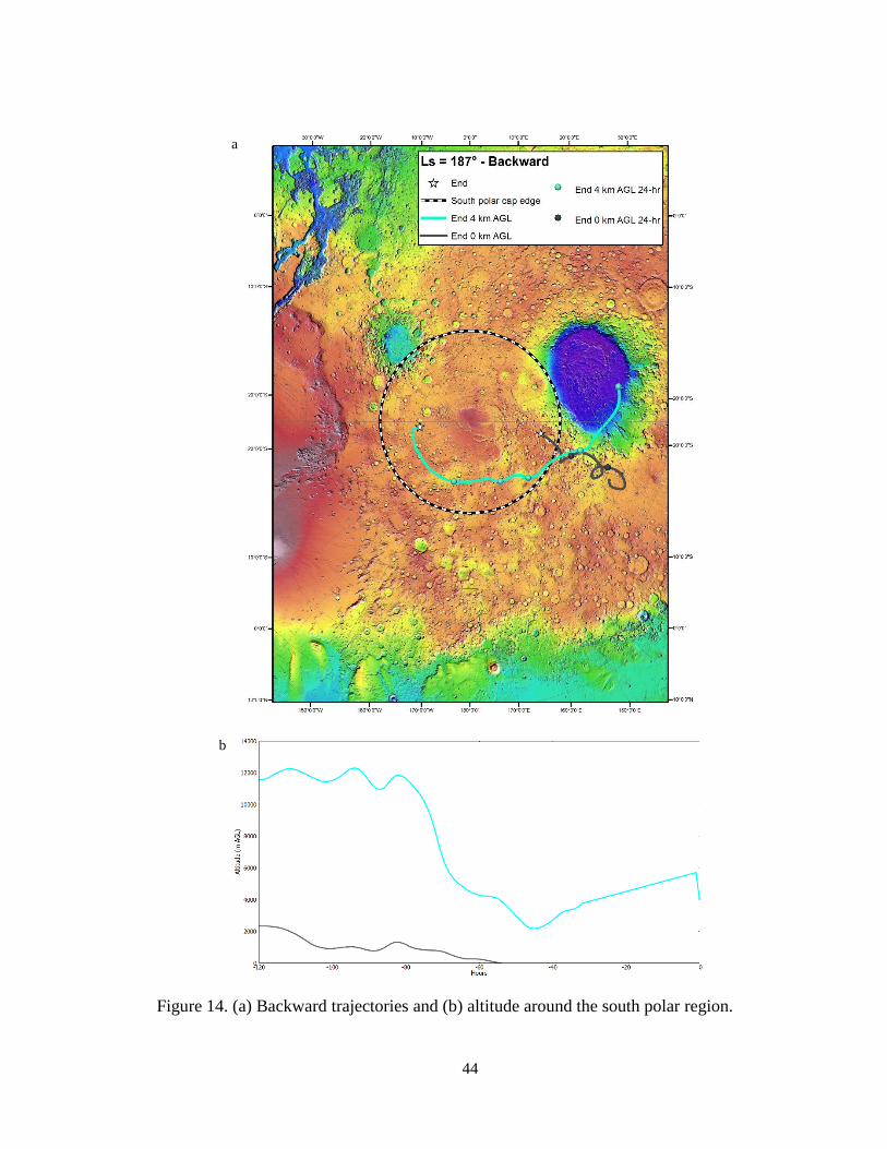
Backward trajectories from the south polar cap verify the source of dust (Figure

14). A trajectory on the opposite side of the south polar cap from Hellas at 4 km AGL

starts at Ls = 187° and is traced back to Ls = 184° (Figure 14a). The trajectory wraps

around the south polar cap back to the eastern side of Hellas from ~12 km AGL at Ls =

184°, corresponding to the observations in Figures 11 and 12. The other trajectory in

Figure 14a starts near Malea Planum at the surface from Ls = 187° and back to Ls = 184°.

As dust hits the surface in Malea Planum within the south polar cap, the parcels originate

from ~2 km AGL in Promethei Terra.

40

Figure 10. (a) Forward trajectories and (b) altitude for the western Hellas region.

a

b

41

Figure 11. As in Figure 10 but for the central Hellas region.

a

b

42

Figure 12. As in Figure 10 but for the eastern Hellas region.

a

b

43

Figure 13. As in Figure 12 but starting at Ls = 188°.

a

b

44

Figure 14. (a) Backward trajectories and (b) altitude around the south polar region.

a

b

45

5.2 Claritas

Forward trajectories from the Claritas region are shown in Figures 15 and 16.

The MGS-MOC topography is shown with an equatorial projection with the latitude for

the south polar cap edge at 55°S, the Tharsis volcanoes located on the left, and Valles

Marineris on the right. The trajectories around Claritas start at higher altitudes as the

result of lower level trajectories immediately descending to the surface.

Figure 15 starts forward trajectories at Ls = 188° since the initial dust activity

around Claritas began at Ls = 188.2°. The parcels at nearly all levels move to the

southeast across Solis Planum and into Aonia Terra (Figure 15a). These parcels ascend

throughout the three sols and remain well above their start point (Figure 15b). The parcel

starting at 3 km is lifted to nearly 12 km by the end of its trajectory.

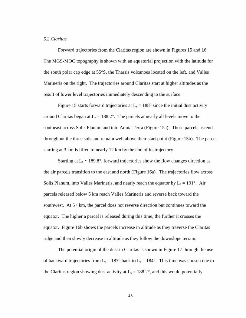
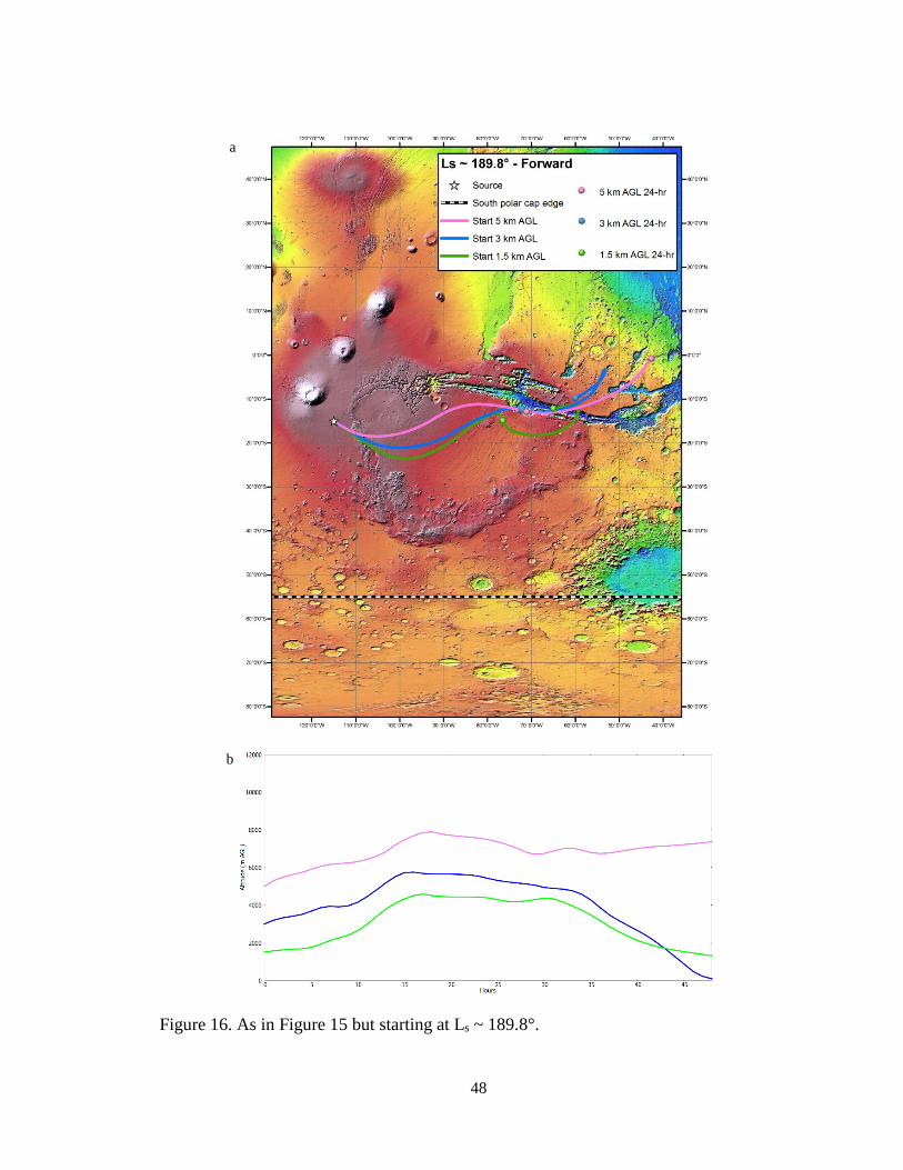
Starting at Ls ~ 189.8°, forward trajectories show the flow changes direction as

the air parcels transition to the east and north (Figure 16a). The trajectories flow across

Solis Planum, into Valles Marineris, and nearly reach the equator by Ls = 191°. Air

parcels released below 5 km reach Valles Marineris and reverse back toward the

southwest. At 5+ km, the parcel does not reverse direction but continues toward the

equator. The higher a parcel is released during this time, the further it crosses the

equator. Figure 16b shows the parcels increase in altitude as they traverse the Claritas

ridge and then slowly decrease in altitude as they follow the downslope terrain.

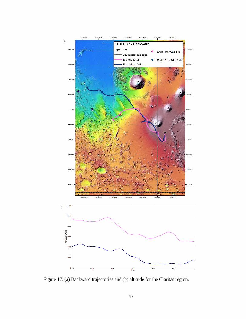
The potential origin of the dust in Claritas is shown in Figure 17 through the use

of backward trajectories from Ls = 187° back to Ls = 184°. This time was chosen due to

the Claritas region showing dust activity at Ls = 188.2°, and this would potentially

46

determine the origin of the observed dust activity. The general direction of flow is from

the northwest near Amazonis Planitia at most levels shown in Figure 17a. In general, the

trajectories begin from a higher altitude and sink into the Claritas region (Figure 17b).

The source of air from the northwest would suggest that the Claritas dust activity was a

result of local lifting and not due to the advection of dust from the Hellas dust storm.

47

Figure 15. (a) Forward trajectories and (b) altitude for the Claritas region.

a

b

48

Figure 16. As in Figure 15 but starting at Ls ~ 189.8°.

a

b

49

Figure 17. (a) Backward trajectories and (b) altitude for the Claritas region.

a

b

50

6. Discussion and Conclusions

HYSPLIT is a reliable and popular model used in several studies to calculate the

transport of aerosols or radionuclides through the Earth’s atmosphere. Previous studies

modified HYSPLIT for the use of specific model data but not for another planet such as

Mars. This study modified the HYSPLIT trajectory prediction model for Mars and

showed its effectiveness in replicating satellite imagery observations of dust movement.

The modified HYSPLIT accounts for the uniqueness of Mars and enables the input of

meteorological data from an MGCM.

Dust plays a crucial role in the atmosphere and climate of Mars, requiring studies

beyond the scope of satellite imagery analysis. The modification of HYSPLIT allows the

study of air parcel motion and consequently dust transport in the Martian atmosphere.

We analyzed the dust transport during the 2001 global dust storm in MY 25 with forward

and backward trajectories. The trajectories presented assume dust has been lifted in the

area for the winds to advect around the planet. In addition, the dust is assumed to remain

aloft and continue along the trajectory without depositing onto the surface. The particular

regions of interest included the observed initial location for the storm from the Hellas

basin impact crater, and the location of a regional dust storm that helped sustain the

global dust storm from Claritas Fossae.

A comparison of MDGM images and trajectories from HYSPLIT provided a

validation of our technique. The comparison of MDGM images and trajectories can be

subject to inconsistencies because the MDGM images are developed from swaths

captured by the MGS-MOC throughout a sol and patched together to span the globe.

51

Based on our analysis, the trajectories starting from the central and eastern

regions of Hellas correlate with the MDGM observations of dust flow to the south from

Hellas. The trajectories then approach the south polar cap edge by Ls ~ 185.2°, and

circulate around the south pole by Ls = 187°. The trajectories starting above 1.5 km

(Figures 11a, 12a) continue around the south polar cap further than suggested by the

MDGM at Ls = 187.24° (Figure 8c). This difference may be a result of the resolution of

the MGCM or because the dust that was advected by the winds had fallen to the surface

prior to this time. Forward trajectories from the western edge of Hellas reveal lower level

parcels sinking to the surface within a sol (Figure 10). This helps explain the

observations of the asymmetric expansion of dust to the east from Hellas instead of to the

west. As a result of the circulation around the south polar cap originating from the center

and eastern edge of Hellas, the source of dust was from these areas of Hellas and not

from the western edge. Forward trajectories starting at Ls = 184° from the eastern edge

of Hellas (Figure 12a) compared with starting at Ls = 188° (Figure 13a) replicate the shift

in wind direction seen on MDGM images. Air parcel trajectories show a flow to the

south at Ls = 184° that changed to a flow to the east by Ls = 188°. The wind shift

occurred because the dust injection from Hellas into the polar region was cut off (Figures

8e, 8f).

Backward trajectories at Ls = 187° from the south polar cap (Figure 14a) show

similar results in Figures 11 and 12 as the dust originated from the eastern side of Hellas

at Ls = 184°. As dust eventually moved east of Hellas into Promethei Terra, backward

trajectories from Malea Planum (Figure 14a) show the dust descending and settling on

52

the south polar cap. As strong storm activity lifts dust from the surface around Hellas,

the dust settling on the south polar cap surface may relate to the PLDs observations.

These trajectories provide evidence for a global dust storm transporting dust to the poles

and possibly contributing to the observed dust layering.

The MDGM images revealed dust activity around Claritas at Ls = 188° but an

important question to address is: was the Claritas dust storm due to local storm activity or

did the dust originate from the expansion of the Hellas dust storm to the east? The

forward trajectories from Hellas at Ls = 188° (Figure 13) reveal air parcels flow to the

east and descend to the surface several kilometers west of Claritas. This evidence

indicates that the dust activity observed around Claritas did not correspond to the dust

activity occurring at Hellas. In addition, backward trajectories starting at Ls = 187° from

Claritas (Figure 17) reveal air parcels coming from the northwest near Amazonis Planitia.

These results suggest the Hellas and Claritas storm activity were independent local

events.

In regards to the Claritas dust storm progression, forward trajectories from Ls =

188° starting at Claritas are comparable to the MDGM observations of a flow to the

southeast into Aonia Terra (Figure 15a). After Ls = 190.5°, the flow changes to the

northeast, crossing the equator probably due to enhanced Hadley cell circulation (Haberle

et al. 1993). Forward trajectories from Ls ~ 189.8° (Figure 16a) follow this pattern to the

northeast with air parcels starting at 5 km and continuing into Lunae Planum. As the

regional dust storm lofted dust to higher altitudes, dust may have been entrained into the

ascending branch of the Hadley cell circulation located in the southern hemisphere at this

53

time (Figure 3a). The dust could then be transported to the north and sink to the surface

in the descending branch of the Hadley cell in the northern hemisphere. This

hemispheric redistribution of dust may have contributed to the dust storm becoming

global.

Uncertainties can be introduced by the assumptions used in this study including

massless dust particles assumed to have been lifted from the surface and following along

the trajectory. Any dust particle has a mass that will cause the particle to fall to the

surface by itself. However, observations show dust can be lofted high in the atmosphere

and remain aloft for long periods of time. The trajectories presented represent the general

flow of dust capable of remaining suspended in the atmosphere. Most large particles

likely fell to the surface prior to the end of their trajectory.

Particular times of air parcel motions were nearly identical to the MDGM images

but variations in the time could be a result of the coarse resolution of the MGCM. The

improvement in the grid spacing of 7.5° latitude and 9° longitude would be advantageous

for future studies to compare to our results. Other possible errors could include

horizontal and vertical interpolation errors of meteorological parameters made in the

HYSPLIT model. The ability of our customized HYPSLIT to replicate observations

made in the MDGM images can help future studies analyze dust transport in the Martian

atmosphere and answer questions concerning dust storm events and the PLDs.

54

REFERENCES

Anderson, E. M., and C. B. Leovy, 1978: Mariner 9 television limb observations of dust

and ice hazes on Mars. J. Geophys. Res., 35, 723-734.

Barlow, N., 2008: Mars: An introduction to its interior, surface, and atmosphere.

Cambridge University Press, 281 pp.

Basu S., M. I. Richardson, and R. J. Wilson, 2004: Simulations of the Martian dust cycle

with the GFDL Mars GCM. J. Geophys. Res., 109, E11006.

Calvin, W. M., and T. M. Martin, 1994: Spatial variability in the seasonal south polar

cap of Mars. J. Geophys. Res., 99, 21143-21152.

Cantor, B. A., 2007: MOC observations of the 2001 Mars planet-encircling dust storm.

Icarus, 186, 60-96.

Cantor, B. A., M. Caplinger, P. James, and M. J. Wolff, 2001: Martian dust storms: 1999

Mars Orbiter Camera observations. J. Geophys. Res., 106, 23653-23687.

Cantor, B. A., and Coauthors, 2008: Observations of the Martian atmosphere by MRO-

MARCI, an overview of 1 Mars year. Third International Workshop on the Mars

atmosphere: Modelling and Observations, Wlliamsburg, Virginia.

Choi, D. S., and C. M. Dundas, 2011: Measurements of Martian dust devil winds with

HiRISE, Geophys. Res. Lett., 38, L24206.

Clancy, R. T., B. Sandor, M. Wolff, P. Christensen, M. Smith, J. Pearl, B. Conrath, and

R.Wilson, 2000: An intercomparison of ground-based millimeter, MGS TES, and

Viking atmospheric temperature measurements- Seasonal and interannual

variability of temperatures and dust loading in the global Mars atmosphere.

J. Geophys. Res., 105, 9553-9571.

Collins, M., and I. N. James, 1995: Regular baroclinic transient waves in a simplified

global circulation model of the Martian atmosphere. J. Geophys. Res., 100,

14421-14432.

Draxler, R. R., 1999: HYSPLIT4 user's guide. NOAA Tech. Memo. ERL ARL-230,

NOAA Air Resources Laboratory, Silver Spring, MD.

Draxler, R. R. and A. D. Taylor, 1982: Horizontal dispersion parameters for long-range

transport modeling. J. Appl. Meteor., 21, 367-372.

Draxler, R. R., and G. D. Hess, 1997: Description of the HYSPLIT_4 modeling system.

55

NOAA Tech. Memo. ERL ARL-224, NOAA Air Resources Laboratory, Silver

Spring, MD, 24 pp.

Draxler, R. R., and G. D. Rolph, 2007: HYSPLIT-WEB Short Course. National Air

Quality Conference, Orlando, Florida.

Draxler, R. R, and G. D. Rolph, 2012: Evaluation of the Transfer Coefficient Matrix

(TCM) approach to model the atmospheric radionuclide air concentrations from

Fukishima. J. Geophys. Res., 117.

Draxler, R. R. and G. D. Rolph, 2015: HYSPLIT (HYbrid Single-Particle Lagrangian

Integrated Trajectory) Model access via NOAA ARL READY Website

(http://ready.arl.noaa.gov/HYSPLIT.php). NOAA Air Resources Laboratory,

Silver Spring, MD.

Draxler, R. R., and Coauthors, 2013: The World Meteorological Organization’s

Evaluation of Meteorological Analyses for the Radionuclide Dispersion and

Deposition from the Fukushima Daiichi Nuclear Power Plant Accident. Third

meeting of WMO on meteorological analyses for Fukushima-Daiichi nuclear

power plant accident. Vienna, Austria.

Dreher, J., 2009: Configuring the HYSPLIT model for National Weather Service

Forecast Office and Spaceflight Meteorology Group Applications. NASA

Contractor Report CR-2009-214764, 36 pp.

Eslinger, P., and Coauthors, 2014: Source Term Estimation of Radioxenon Released from

the Fukushima Dai-Ichi Nuclear Reactors Using Measured Air Concentrations

and Atmospheric Transport Modeling. Journal of Environmental Radioactivity,

127, 127-132.

Fenton, L. K., and M. I. Richardson, 2001: Martian surface winds: Insensitivity to orbital

changes and implications for aeolian processes. J. Geophys. Res., 106, 32,885-

32,902.

Giuranna, M., G. Hansen, V. Formisano, L. Zasova, A. Maturilli, D. Grassi, and N.

Ignatiev, 2007: Spatial variability, composition, and thickness of the seasonal

north polar cap of mars in mid-spring. Planetary and Space Science, 55, 1328-

1345.

Haberle, R. M., J. B. Pollack, J. R. Barnes, R. W. Zurek, C. B. Leovy, J. Murphy, H. Lee,

and J. Schaeffer, 1993: Mars Atmospheric Dynamics as Simulated by the NASA

Ames General Circulation Model 1. The Zonal-Mean Circulation. J. Geophys.

Res., 98, 3093-3123.

56

Hess, S. L., R. M. Henry, C. B. Leovy, J. A. Ryan, and J. E. Tillman, 1977:

Meteorological results from the surface of Mars: Viking 1 and 2, J. Geophys.

Res., 82, 4559-4574.

Hourdin, F., 1992: A new representation of the CO2 15μm band for a Martian general

circulation model. J. Geophys. Res., 97, 18319-18335.

Housiadas, C., 1999: Cm-hysplit: A software capability forresponse in nuclear

emergencies. Tech. rep., Institute of Nuclear Technology and Radiation

Protection.

Hvidberg, C. S., K. E. Fishbaugh, M. Winstrup, A. Svensson, S. Byrne, and K. E.

Herkenhoff, 2012: Reading the climate record of the martian polar layered

deposits. Icarus, 221, 405-419.

Jakosky, B. M., and Coauthors, 2015: The Mars Atmosphere and Volatile Evolution

(MAVEN) Mission. Space Sci. Rev.

Kahanpää, H., and Coauthors, 2014: Convective vortices at the MSL landing site. Fifth

International Workshop on the Mars atmosphere: Modelling and Observations,

Oxford, UK.

Kahre, M. A., and R. M. Haberle, 2010: Mars CO2 cycle: Effects of airborne dust and

polar cap ice emissivity. Icarus, 207, 648-653.

Kahre, M. A., J. R. Murphy, and R. M. Haberle, 2006: Modeling the Martian dust cycle

and surface dust reservoirs with the NASA Ames general circulation model.

J. Geophys. Res., 111, E06008.

Kieffer, H. H., B. M. Jakosky, C. W. Snyder, and M. S. Matthews, 1992: Mars. The

University of Arizona Press, 1498 pp.

Leovy, C., 2001: Weather and climate on Mars. Nature, 412, 245-249.

Leovy, C. B., and Y. Mintz, 1969: Numerical simulations of the atmospheric circulation

and climate of Mars. J. Geophys. Res., 26, 1167-1190.

Magalhães, J. A., J. T. Schofield, and A. Seiff, 1999: Results of the Mars Pathfinder

atmospheric structure investigation. J. Geophys. Res., 104, 8943-8955.

Martin, T. Z., and R. W. Zurek 1993: An analysis of the history of dust activity on Mars.

J. Geophys. Res., 98, 3221-3246.

Montabone, L., and Coauthors, 2015: Eight-year Climatology of Dust Optical Depth on

57

Mars. Icarus, 251, 65-95.

Murray, B. C., L. A. Soderblom, J. A. Cutts, R. P. Sharp, D. J. Milton, and R. B.

Leighton, 1972: Geological framework of the south polar layered region of Mars.

Icarus, 17, 328-345.

Noble, J., 2013: Integration of Mars Global Surveyor observations of the MY 25 planet-

encircling dust storm on Mars: implications for atmospheric dynamics and

modeling. M. S. thesis, Department of Meteorology and Climate Science, San

José State University, 116 pp.

Read, P. L., and S. R. Lewis, 2004: The Martian climate revisited: atmosphere and

environment of a desert planet. Springer-Praxis Books, 326 pp.

Reiss, D., A. Spiga, and G. Erkeling, 2014: The horizontal motion of dust devils on Mars

derived from CRISM and CTX/HiRISE observations. Icarus, 227, 8-20.

Richardson, M. I., and R. J. Wilson, 2002: A topographically forced asymmetry in the

martian circulation and climate. Nature, 416, 298-301.

Rolph, G. D., 2015. Real-time Environmental Applications and Display sYstem

(READY) Website (http://ready.arl.noaa.gov). NOAA Air Resources Laboratory,

Silver Spring, MD.

Ryan, J. A., and R. M. Henry, 1979: Mars Atmospheric Phenomena During Major Dust

Storms, as Measured at Surface. J. Geophys. Res., 84, 2821-2829.

Ryan, J. A., and R. D. Lucich, 1983: Possible Dust Devils, Vortices on Mars. J. Geophys.

Res., 88, 11,005-11,011.

Schofield, J., and Coauthors, 1997: The Mars Pathfinder atmospheric structure

investigation/meteorology (ASI/MET) experiment. Science, 278, 1752-1758.

Smith, D. E., and Coauthors, 2001: Mars Orbiter Laser Altimeter: Experiment summary

after the first year of global mapping of Mars. J. Geophys. Res., 106, 23,689-

23,722.

Smith, M. D., 2009: THEMIS observations of Mars aerosol optical depth from 2002-

2008. Icarus, 202, 444-452.

Smith, M. D., B. J. Conrath, J. C. Pearl, and P. R. Christensen, 2002: Thermal Emission

Spectrometer Observations of Martian Planet-Encircling Dust Storm 2001A.

Icarus, 157, 259-263.

58

Stanzel, C. M., M. Pätzold, D. A. Williams, P. L. Whelley, R. Greeley, G. Neukum, and

The HRSC Co-Investigator Team, 2008: Dust devil speeds, directions of motion

and general characteristics observed by the Mars Express High Resolution Stereo

Camera, Icarus, 197, 39-51.

Strausberg, M. J., H. Wang, M. I. Richardson, S. P. Ewald, and A. D. Toigo, 2005:

Observations of the initiation and evolution of the 2001 Mars global dust storm.

J. Geophys. Res., 110, E02006.

Sutton, J. L., C. B. Leovy, and J. E. Tillman, 1978: Dirunal variations of the martian

surface layer meteorological parameters during the first 45 sols at two Viking

Lander sites. J. Geophys. Res., 35, 2346-2355.

Takahashi, Y. O., H. Fujiwara, H. Fukunishi, M. Odaka, Y. Hayashi, and S. Watanabe,

2003: Topographically induced north-south asymmetry of the meridional

circulation in the Martian atmosphere. J. Geophys. Res., 108, 5018.

Vasavada, A. R., and Coauthors, 2014: Overview of the Mars Science Laboratory

mission: Bradbury Landing to Yellowknife Bay and beyond. J. Geophys. Res.

Planets, 119, 1134-1161.

Wang, H., and A. P. Ingersoll, 2002. Martian clouds observed by Mars Global Surveyor

Mars Orbiter Camera. J. Geophys. Res., 107, 5078.

Wang, H., and M. I. Richardson, 2015: The origin, evolution, and trajectory of large dust

storms on Mars during Mars years 24-30 (1999-2011). Icarus, 251, 112-127.

Wilson, R. J., and K. Hamilton, 1996: Comprehensive model simulation of thermal tides

in the Martian atmosphere. J. Geophys. Res., 53, 1290-1326.

Zalucha, A. M., 2014: The effect of dust on the Martian Hadley cells. Fifth

International Workshop on the Mars atmosphere: Modelling and Observations,

Oxford, UK.

Zalucha, A. M., R. Plumb, and R. J. Wilson, 2010: An Analysis of the Effect of

Topography on the Martian Hadley Cells. J. Geophys. Res., 67, 673–693.

Zuber, M. T., D. E. Smith, S. C. Solomon, D. O. Muhleman, J. W. Head, B. Garvin, J. B.

Abshire, and J. L. Bufton, 1992: The Mars Observer Laser Altimeter

Investigation. J. Geophys. Res., 97, 7781-7797.

Zurek, R. W., 1982: Martian great dust storms: An update, Icarus, 50, 288-310.

Zurek, R. W., and L. J. Martin, 1993: Interannual variability of planet-encircling dust

59

storms on Mars. J. Geophys. Res., 98, 3247-3259.

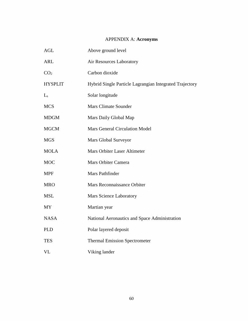
60

APPENDIX A: Acronyms

AGL Above ground level

ARL Air Resources Laboratory

CO2 Carbon dioxide

HYSPLIT Hybrid Single Particle Lagrangian Integrated Trajectory

Ls Solar longitude

MCS Mars Climate Sounder

MDGM Mars Daily Global Map

MGCM Mars General Circulation Model

MGS Mars Global Surveyor

MOLA Mars Orbiter Laser Altimeter

MOC Mars Orbiter Camera

MPF Mars Pathfinder

MRO Mars Reconnaissance Orbiter

MSL Mars Science Laboratory

MY Martian year

NASA National Aeronautics and Space Administration

PLD Polar layered deposit

TES Thermal Emission Spectrometer

VL Viking lander

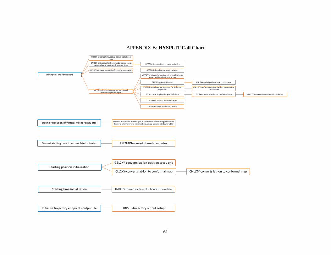
61

APPENDIX B: HYSPLIT Call Chart

Starting time and # of locations

TMINIT-initialize time, set up accumulated days table

DATSET-date setup for basic model parameters, set number of locations & starting time

DECODI-decodes integer input variables

RUNSET-set basic simulation & control parameters DECODR-decodes real input variables

METINI-initialize information about each meteorological data grid

METSET-reads and unpacks meteorological index record and initalize file structure

GBLSET-global grid setup GBLDXY-global grid size by x,y coordinate

STLMBR-initialize map structure for different projections

CNLLXY-tranformation from lat-lon to canonical coordinates

STCM1P-use single point grid definition CLL2XY-converts lat-lon to conformal map CNLLXY-converts lat-lon to conformal map

TM2MIN-converts time to minutes

TM2DAY-converts minutes to time

Define resolution of vertical meteorology grid METLVL-determines internal grid to interpolate meteorology input data levels to internal levels, initialize time, set up accumulated days table

Convert starting time to accumulated minutes TM2MIN-converts time to minutes

Starting position initialization

GBL2XY-converts lat-lon position to x-y grid

CLL2XY-converts lat-lon to conformal map CNLLXY-converts lat-lon to conformal map

Starting time initialization TMPLUS-converts a date plus hours to new date

Initialize trajectory endpoints output file TRJSET-trajectory output setup

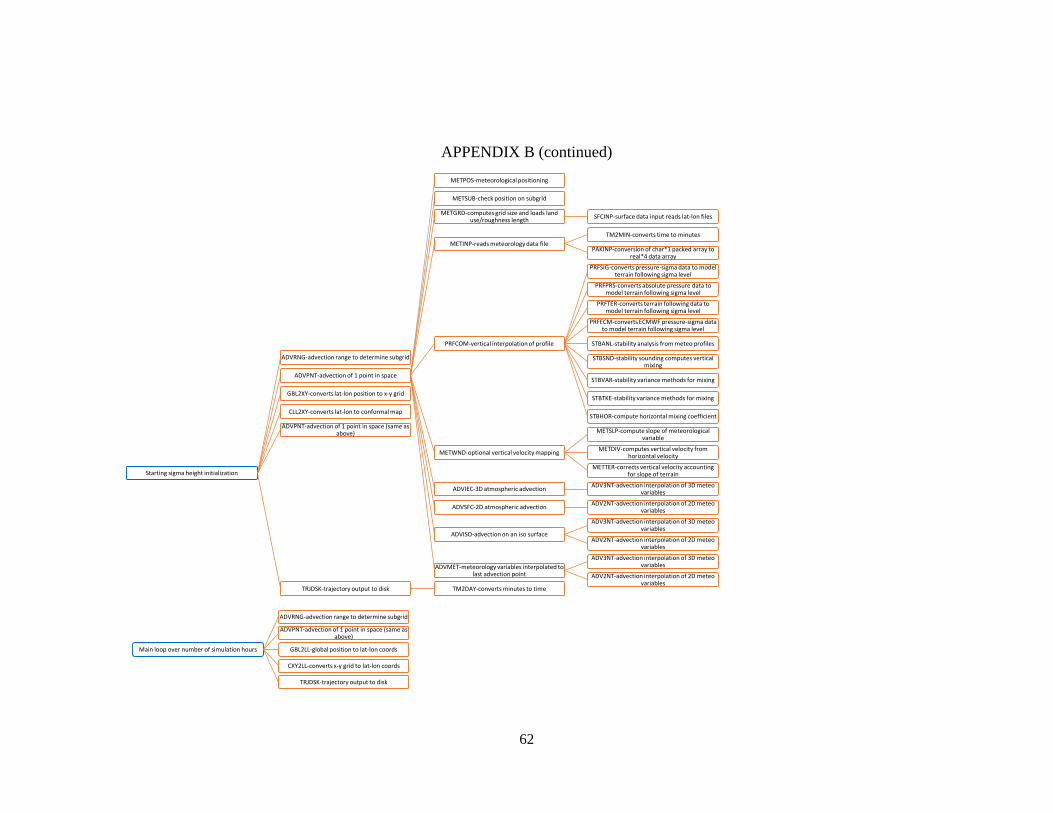
62

APPENDIX B (continued)

Starting sigma height initialization

ADVRNG-advection range to determine subgrid

ADVPNT-advection of 1 point in space

METPOS-meteorological positioning

METSUB-check position on subgrid

METGRD-computes grid size and loads land use/roughness length

SFCINP-surface data input reads lat-lon files

METINP-reads meteorology data file

TM2MIN-converts time to minutes

PAKINP-conversion of char*1 packed array to real*4 data array

PRFCOM-vertical interpolation of profile

PRFSIG-converts pressure-sigma data to model terrain following sigma level

PRFPRS-converts absolute pressure data to model terrain following sigma level

PRFTER-converts terrain following data to model terrain following sigma level

PRFECM-converts ECMWF pressure-sigma data to model terrain following sigma level

STBANL-stability analysis from meteo profiles

STBSND-stability sounding computes vertical mixing

STBVAR-stability variance methods for mixing

STBTKE-stability variance methods for mixing

STBHOR-compute horizontal mixing coefficient

METWND-optional vertical velocity mapping

METSLP-compute slope of meteorological variable

METDIV-computes vertical velocity from horizontal velocity

METTER-corrects vertical velocity accounting for slope of terrain

ADVIEC-3D atmospheric advectionADV3NT-advection interpolation of 3D meteo

variables

ADVSFC-2D atmospheric advectionADV2NT-advection interpolation of 2D meteo

variables

ADVISO-advection on an iso surface

ADV3NT-advection interpolation of 3D meteo variables

ADV2NT-advection interpolation of 2D meteo variables

ADVMET-meteorology variables interpolated to last advection point

ADV3NT-advection interpolation of 3D meteo variables

ADV2NT-advection interpolation of 2D meteo variables

GBL2XY-converts lat-lon position to x-y grid

CLL2XY-converts lat-lon to conformal map

ADVPNT-advection of 1 point in space (same as above)

TRJDSK-trajectory output to disk TM2DAY-converts minutes to time

Main loop over number of simulation hours

ADVRNG-advection range to determine subgrid

ADVPNT-advection of 1 point in space (same as above)

GBL2LL-global position to lat-lon coords

CXY2LL-converts x-y grid to lat-lon coords

TRJDSK-trajectory output to disk