Embed Size (px)
Citation preview

Training Exercises
Exercise Setup
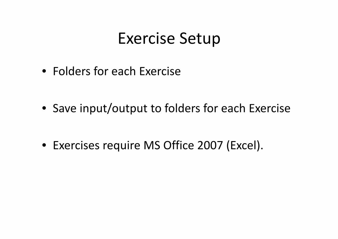
• Folders for each Exercise
• Save input/output to folders for each Exercise
• Exercises require MS Office 2007 (Excel).

Exercise #1: Daily Emissions Inventory
• Problem: This exercise will generate an average daily emissions inventory for Hong Kong for calendar year 2030. Assume model defaults, except as noted below. I/M programs begin in 2014.
• Purpose: familiarization with emission inventories; using BURDEN output formats
• Scenario input data: – Geographic Area: Hong Kong SAR– Calendar Years: 2030– No Alternate Baseline Year– Season: Annual– Scenario Type: BURDEN– Output File types: Detailed Planning Inventory (CSV), MVEI7G (BCD)– Output Frequency: daily– Pollutants: PM10, VOC

Exercise #1: Notes
• Requires 1 scenario for calendar year 2030• Save Input File As: HK_2030_Burden.inp

Exercise #1: Input 1 Tab

Exercise #1: Mode and Output Tab
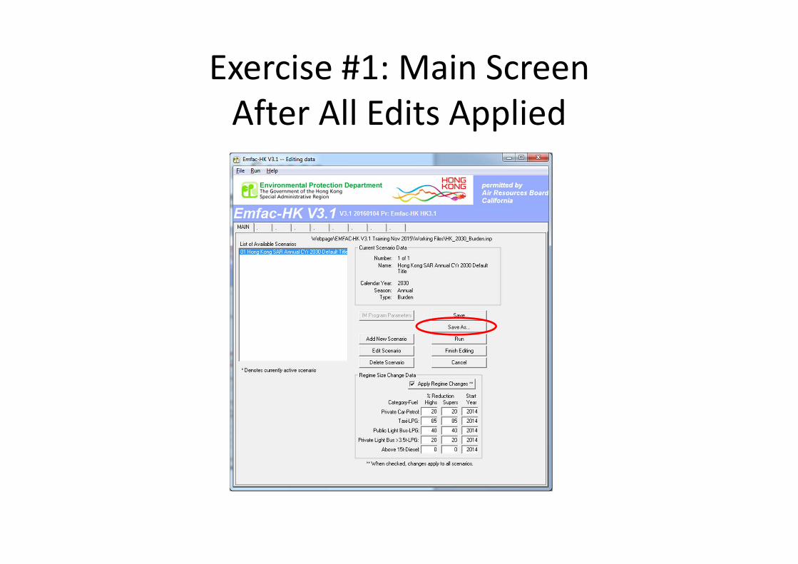
Exercise #1: Main Screen After All Edits Applied
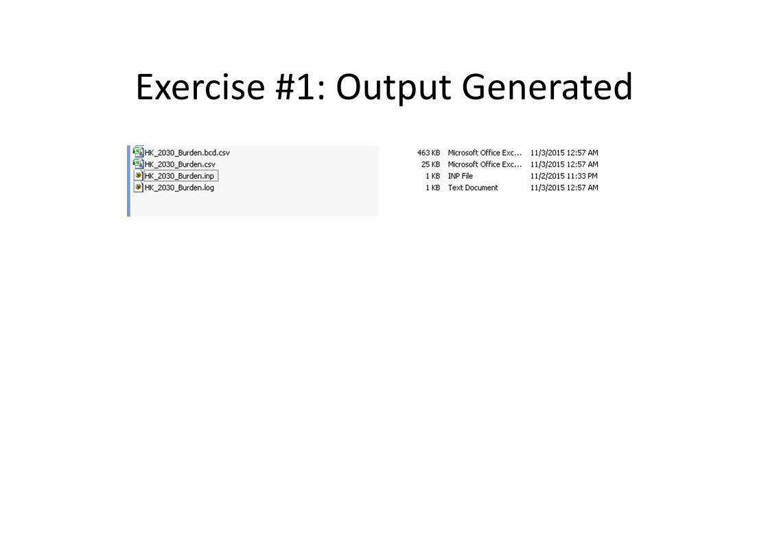
Exercise #1: Output Generated

Exercise #1: Format of the BURDEN Text File with *.CSV extension

Exercise #1: Format of the MVEI7G File with *.BCD.CSV Extension

Exercise #1a: Processing BCD Output
• Problem: using BCD output from Exercise #1, determine total NOx running exhaust emissions for 2030.
• Purpose: post processing of BCD output, single year scenario
• Hints:– Import *.BCD.CSV directly into spreadsheet– Use data filters
• pollutant (NOx), process (“Run Exh”) – Copy filtered results to a separate tab in spreadsheet for analysis
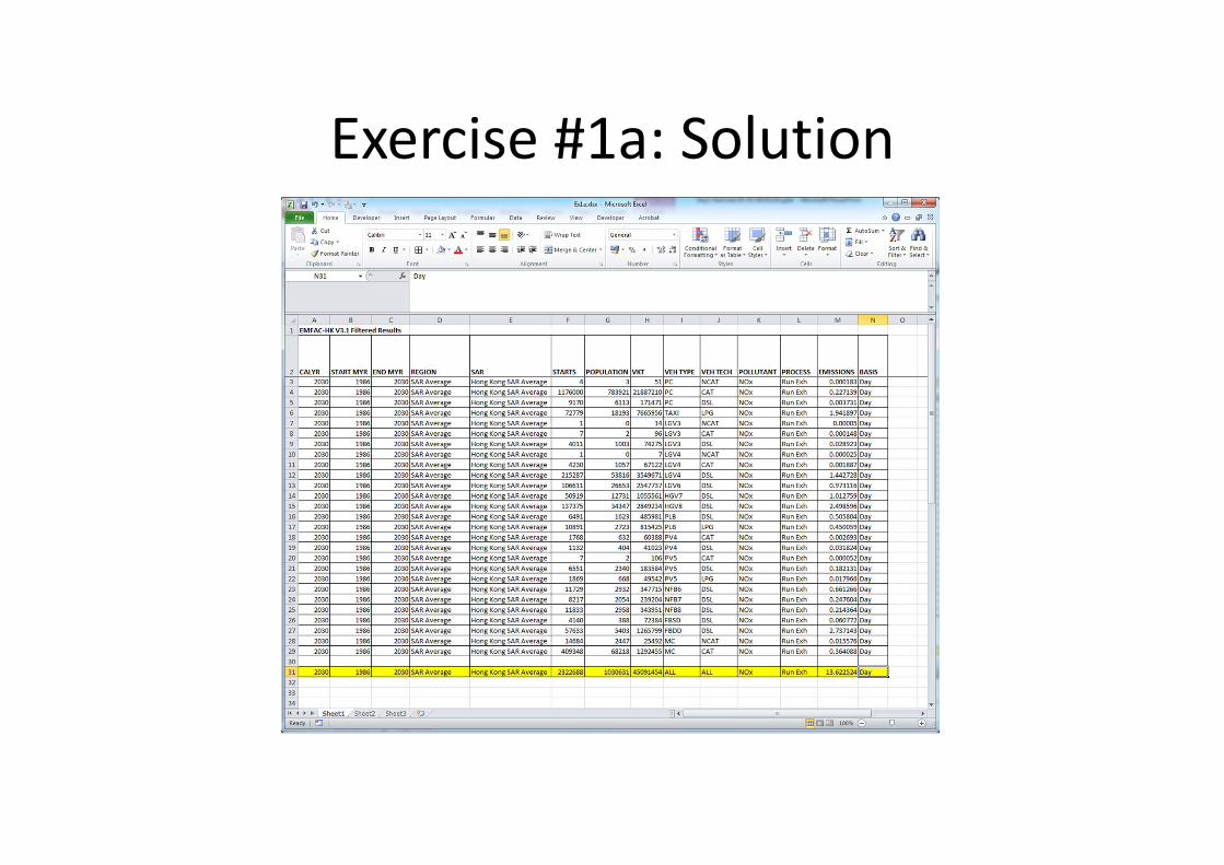
Exercise #1a: Solution
Exercise #1b: Processing Text/CSV Output
• Problem: using Text/CSV output from Exercise #1, determine total NOx running exhaust emissions for 2030.
• Post processing of Text/CSV output

Exercise #1b: Processing Text/CSV Output
Exercise #1c: Determine Fleet‐Average Emissions
• Problem: using spreadsheet results obtained in Exercise #1a, determine the fleet‐average NOxemission factor (gram/km) for all vehicles for 2030.
• Purpose: Convert emission rate to an emission factor
• Steps– Divide EMISSIONS Column by VKT Column– Sum over all vehicle classes to get composite.– Convert units to obtain grams/km

Exercise #1c: Solution
Exercise #2: Hourly Emissions Inventory
• Problem: Repeat Exercise #1, except generate an hourly emissions estimates for Hong Kong for calendar year 2030 only.
• Context: This output is useful to ambient air quality modelers who are interested in hourly emission estimates.
• Scenario data: – Geographic Area: Hong Kong SAR– Calendar Years: 2030– Season: Annual– Scenario Type: BURDEN– Output File types: Text (CSV), BCD– Output Frequency: hourly– Pollutants: PM10, VOC
• Purpose: generating/processing BURDEN hourly output formats

Exercise #2: Hourly Emissions Estimates
• Problem: Repeat Exercise #1, except generate an hourly emissions inventory for Hong Kong for calendar year 2030 only.
• Purpose: generating/processing BURDEN hourly output formats
• Context: This output is useful to ambient air quality modelers who are interested in hourly emission inventories.
• In this run the Burden inventories are calculated on an hourly basis, and then aggregated to show an inventory for the entire day. The hourly inventories are mainly based on disaggregating daily activity to an hourly basis. The data provide default diurnal distribution of hourly trip starts, and vehicle kilometers travelled.
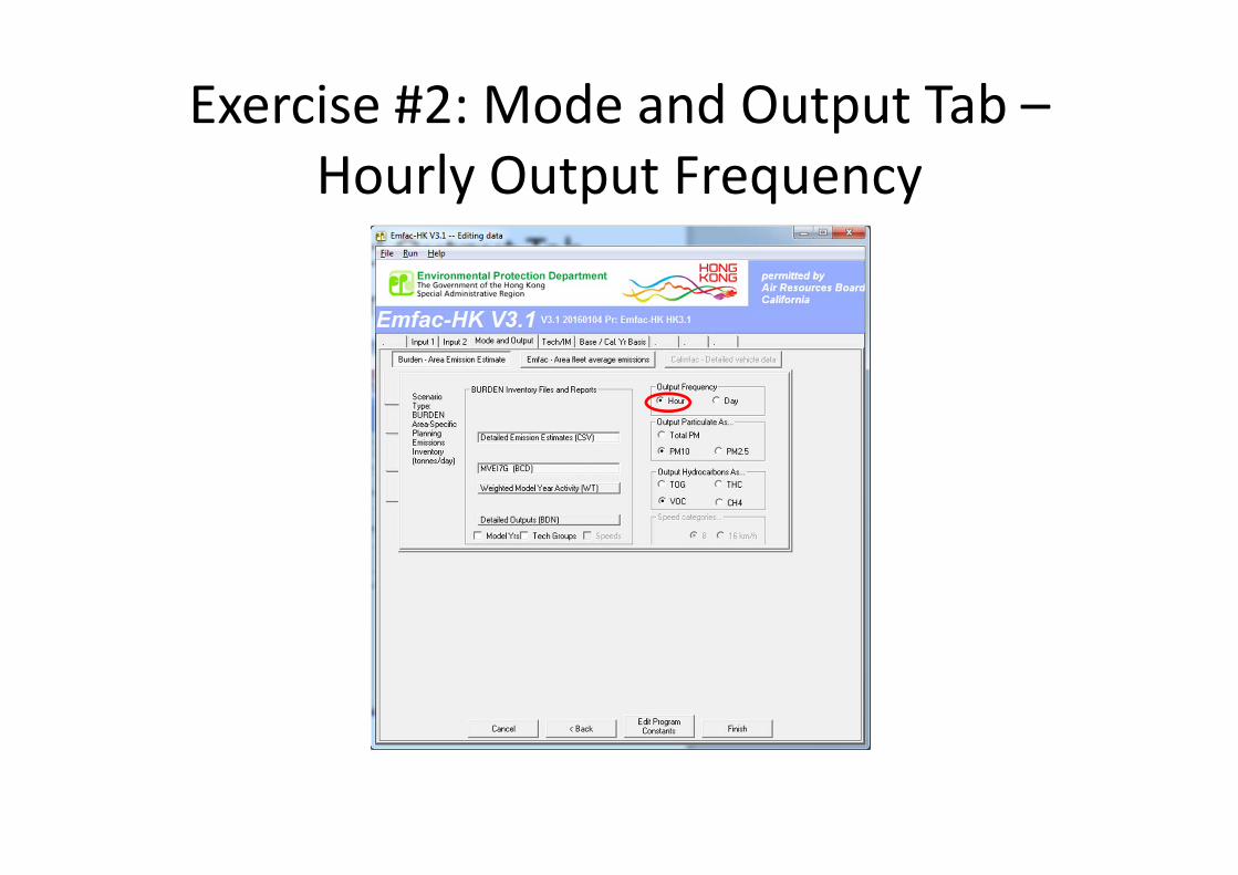
Exercise #2: Mode and Output Tab –Hourly Output Frequency
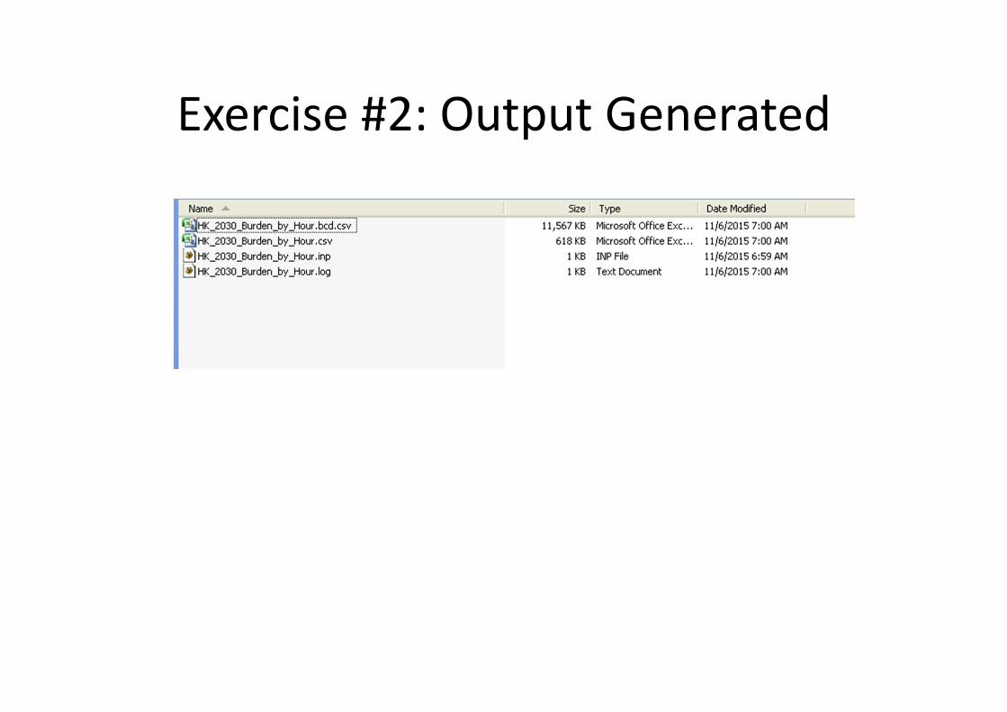
Exercise #2: Output Generated
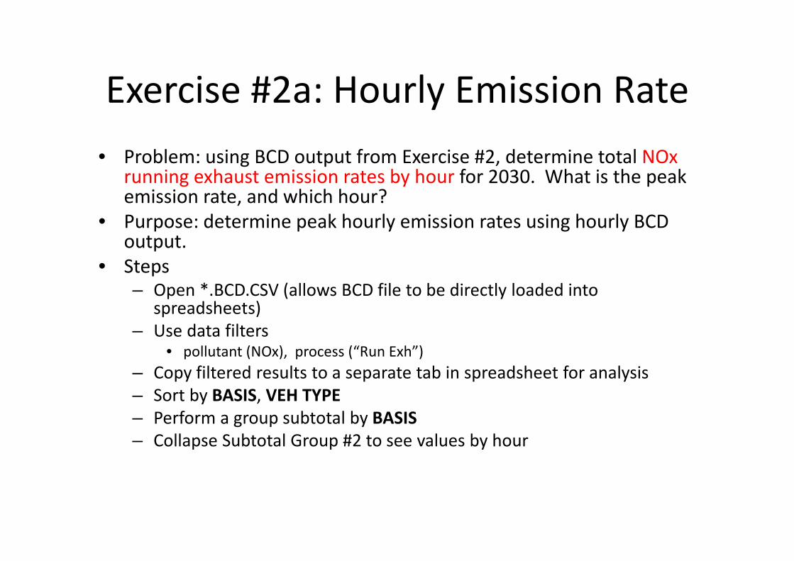
Exercise #2a: Hourly Emission Rate• Problem: using BCD output from Exercise #2, determine total NOx
running exhaust emission rates by hour for 2030. What is the peak emission rate, and which hour?
• Purpose: determine peak hourly emission rates using hourly BCD output.
• Steps– Open *.BCD.CSV (allows BCD file to be directly loaded into
spreadsheets)– Use data filters
• pollutant (NOx), process (“Run Exh”) – Copy filtered results to a separate tab in spreadsheet for analysis– Sort by BASIS, VEH TYPE– Perform a group subtotal by BASIS– Collapse Subtotal Group #2 to see values by hour

Exercise #2a: Solution
Exercise #3: EMFAC Mode
• Problem: Generate emission factors for 25 ºC and 40% RH for calendar year 2030 using the EMFAC mode.
• Context: In Emfac mode the model calculates emission factors either in grams per hour or grams per kilometer for each temperature, relative humidity and average speed combination specified by the user.
• fleet‐average emission factors (grams/km or g/mile) are useful in roadway modeling

Exercise #3: EMFAC Mode
• Scenario data: – Geographic Area: Hong Kong SAR– Calendar Years: 2030– No Alternate Baseline Year– Season: Annual– Scenario Type: EMFAC– Output File types: Impact Rate Detail (RTL)– Temperatures: 25 ºC– Relative Humidity: 40%– Pollutants: PM10, VOC
• Purpose: generating/processing EMFAC formats

Exercise #3: Input 1 Tab (populated)
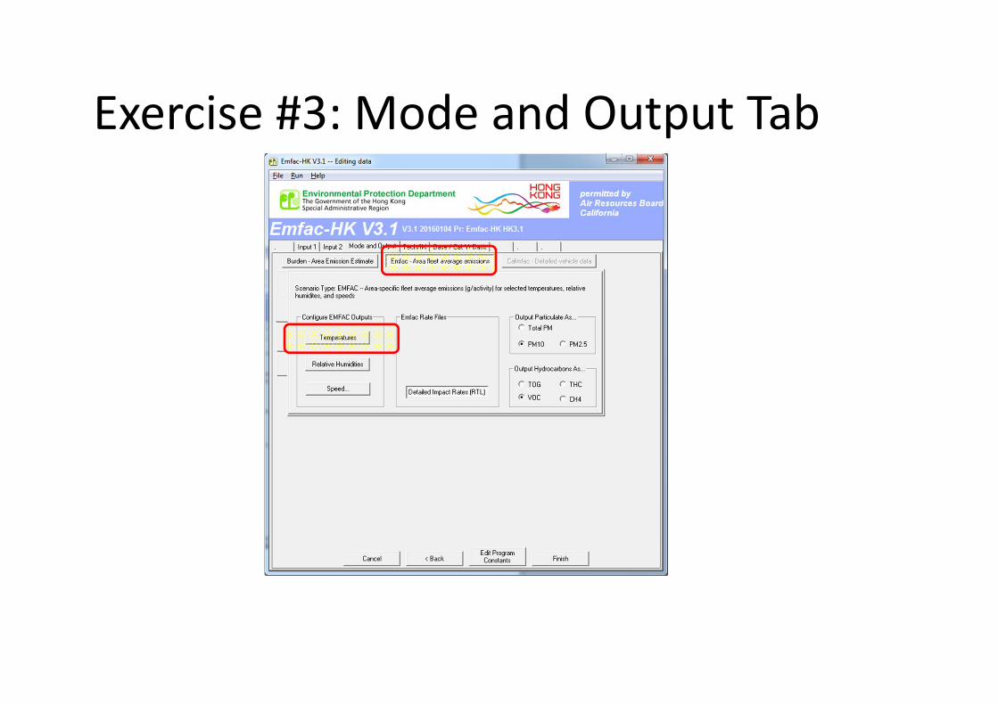
Exercise #3: Mode and Output Tab
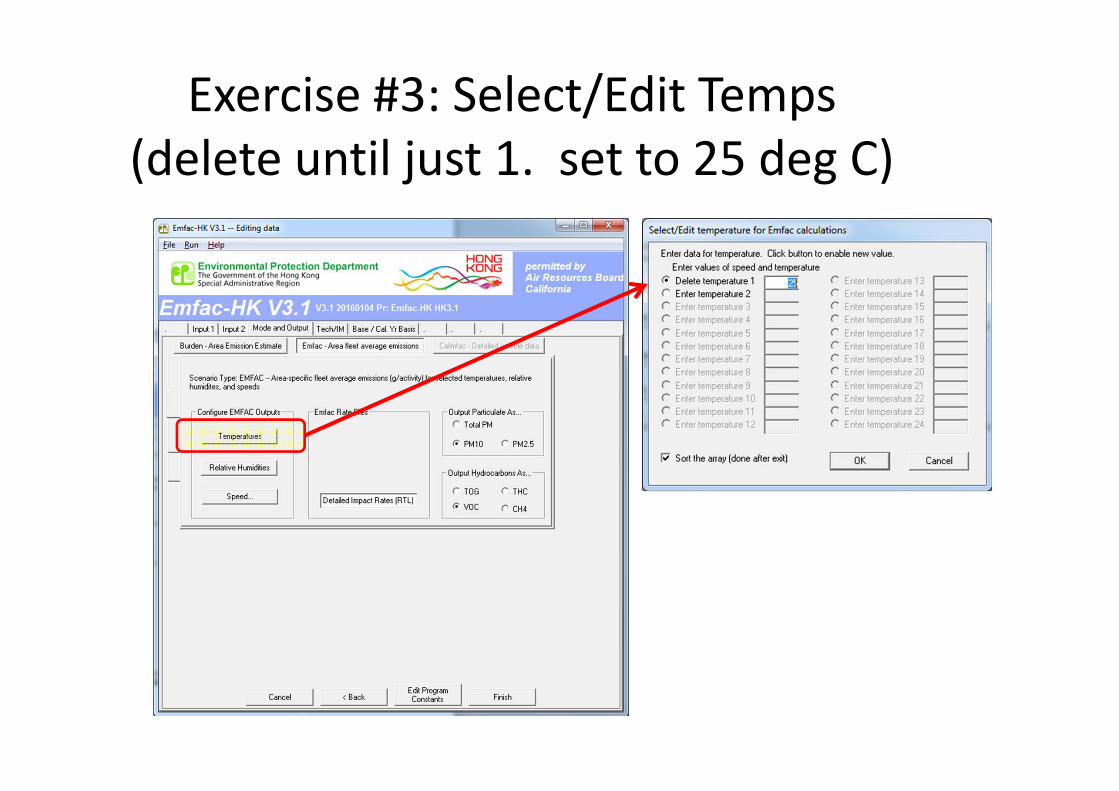
Exercise #3: Select/Edit Temps(delete until just 1. set to 25 deg C)

Exercise #3: Select/Edit RH(delete until just 1. set to 40%)
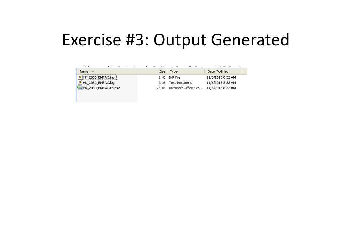
Exercise #3: Output Generated

Exercise #4: Changing Technology Group Fractions
• Context: This example evaluates emission changes if the Government introduces a tax incentive program. In this case, introducing Euro V in 2010 for light goods vehicles greater than 3.5 tonnes (vehicle class LGV6).
• The table below shows the accelerate phase‐in of Euro V for LGV6– Model Year: 2010‐2012 40% Euro V– Model Year: 2013+ 100%

Exercise #4: Changing TG Fractions
• Scenario data: – Geographic Area: Hong Kong SAR– Calendar Years: 2030– Season: Annual– Scenario Type: BURDEN– Output File types: Detailed Estimates (CSV)– Output Frequency: daily– Pollutants: PM10, VOC
• Perform a Base Case Run• Update TG distribution using data on next slide

Exercise #4: New LGV6 Exhaust TG Fractions to Apply
Exh TG ‐> 119 132 133
ModelYear
Euro IV POC LGV 3.5-5-5t Dsl
Euro IV DPF LGV 3.5-5-5t Dsl
Euro V DPF LGV 3.5-5-5t Dsl
2010 17.435% 42.5646% 40%
Source: http://www.epd.gov.hk/epd/sites/default/files/epd/2013_Licensed_Vehicle_by_Age_and_Technology_Group_Fractions.xls
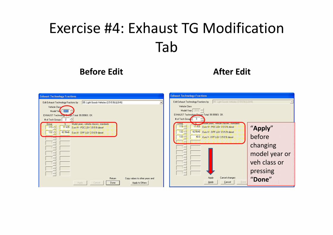
Exercise #4: Exhaust TG Modification Tab
Before Edit After Edit
“Apply” before changing model year or veh class or pressing “Done”

Exercise #4: “Apply to Others – Model Year Only”
Before Edit After Edit
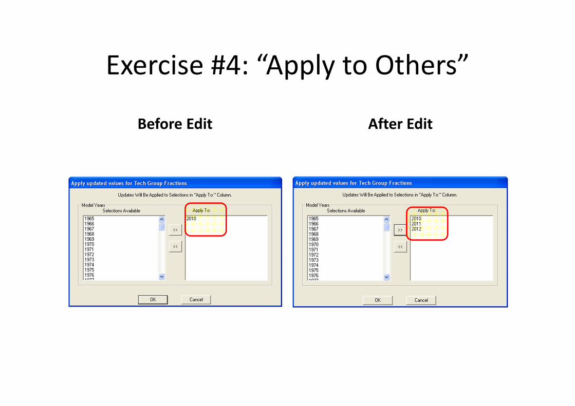
Exercise #4: “Apply to Others”
Before Edit After Edit
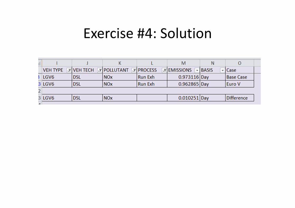
Exercise #4: Solution
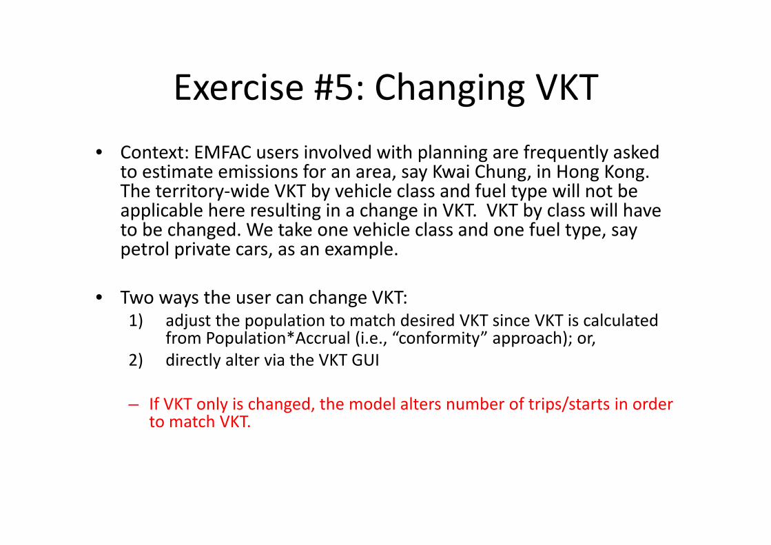
Exercise #5: Changing VKT• Context: EMFAC users involved with planning are frequently asked
to estimate emissions for an area, say Kwai Chung, in Hong Kong. The territory‐wide VKT by vehicle class and fuel type will not be applicable here resulting in a change in VKT. VKT by class will have to be changed. We take one vehicle class and one fuel type, say petrol private cars, as an example.
• Two ways the user can change VKT: 1) adjust the population to match desired VKT since VKT is calculated
from Population*Accrual (i.e., “conformity” approach); or,2) directly alter via the VKT GUI
– If VKT only is changed, the model alters number of trips/starts in order to match VKT.

Exercise #5: Changing VKT
• Problem: Determine emissions in 2030 for petrol private cars (Vehicle Class 1) given a forecasted VKT of 1,609,000 km/day.
• This Exercise will be conducted in three phases: – 5: “base” case– 5a: “conformity” adjustment– 5b: direct VKT adjustment

Exercise #5a: Changing VKT (“Conformity” Approach)
• Scenario data: – Geographic Area: Hong Kong SAR– Calendar Years: 2030– Season: Annual– Scenario Type: BURDEN– Output File types: Text (CSV), BCD– Output Frequency: hourly– Pollutants: PM10, VOC
• VKT for private cars = 1,609,000 km/day
• Use “conformity” approach: adjust population to match desired VKT

Exercise #5a: Notes• Determine Population Adjustment to Match VKT
– Find “base” population and VKT for vehicle class and fuel for 2030.
• Enter scenario data in Input 1 screen • Edit Program Constants • Click “Population” key in Tab Pop/Accrual Screen
– Select By Vehicle and Fuel: – PC petrol population? (Vehicle Class 1, Fuel=1):
• Advance to VKT Screen – Tab By Vehicle and Fuel:– PC VKT (Vehicle Class=1, Fuel=1)?:
– Determine VKT adjustment factor?
• Multiply population by VKT adjustment factor:
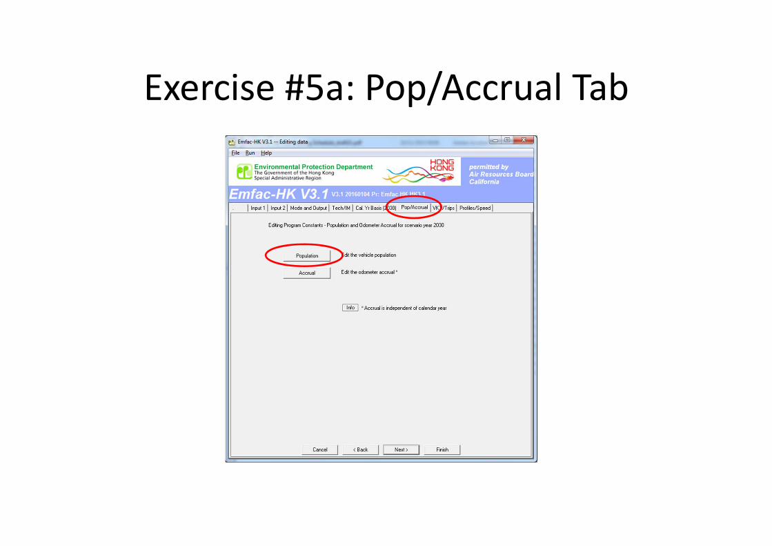
Exercise #5a: Pop/Accrual Tab

Exercise #5a: VKT/Trips Tab
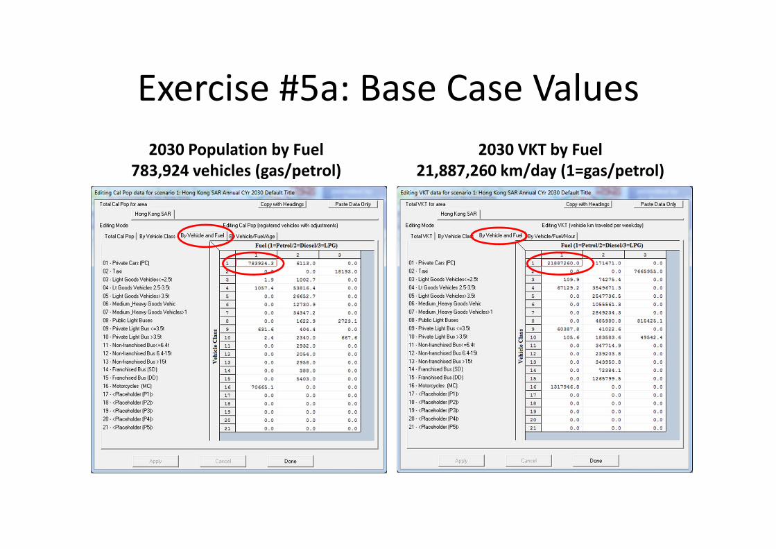
Exercise #5a: Base Case Values2030 Population by Fuel
783,924 vehicles (gas/petrol)2030 VKT by Fuel
21,887,260 km/day (1=gas/petrol)

Exercise #5a: VKT Adjustment using Population
• Find “base” population and VKT for vehicle class and fuel (PC petrol) for 2030: – Population (2030): 783,924 vehicles– VKT (2030 base): 21,887,260 kilometers
• Determine VKT adjustment factor:– 1,609,000/ 21,887,260 = 0.0735
• Multiply population by factor:– 783,924 * 0.0735 = 57,629
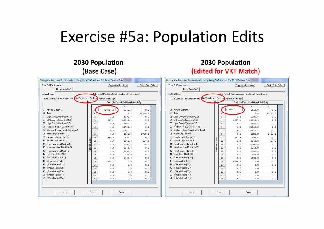
Exercise #5a: Population Edits2030 Population
(Base Case)2030 Population
(Edited for VKT Match)

Exercise #5a: Verify VKT Adjustment2030 VKT (Base Case)
2030 VKT(After Pop Edit)

Exercise #5b: Changing VKT (Directly)
• Problem: Determine emissions in 2030 for petrol private cars (Vehicle Class 1) given a forecasted VKT of 1,609,000 km/day.
• Scenario data: – Geographic Area: Hong Kong SAR– Calendar Years: 2030– Season: Annual– Scenario Type: BURDEN– Output File types: Text (CSV), BCD– Output Frequency: hourly– Pollutants: PM10, VOC
• VKT for petrol private cars = 1,609,000 km/day
• Direct entry of new VKT
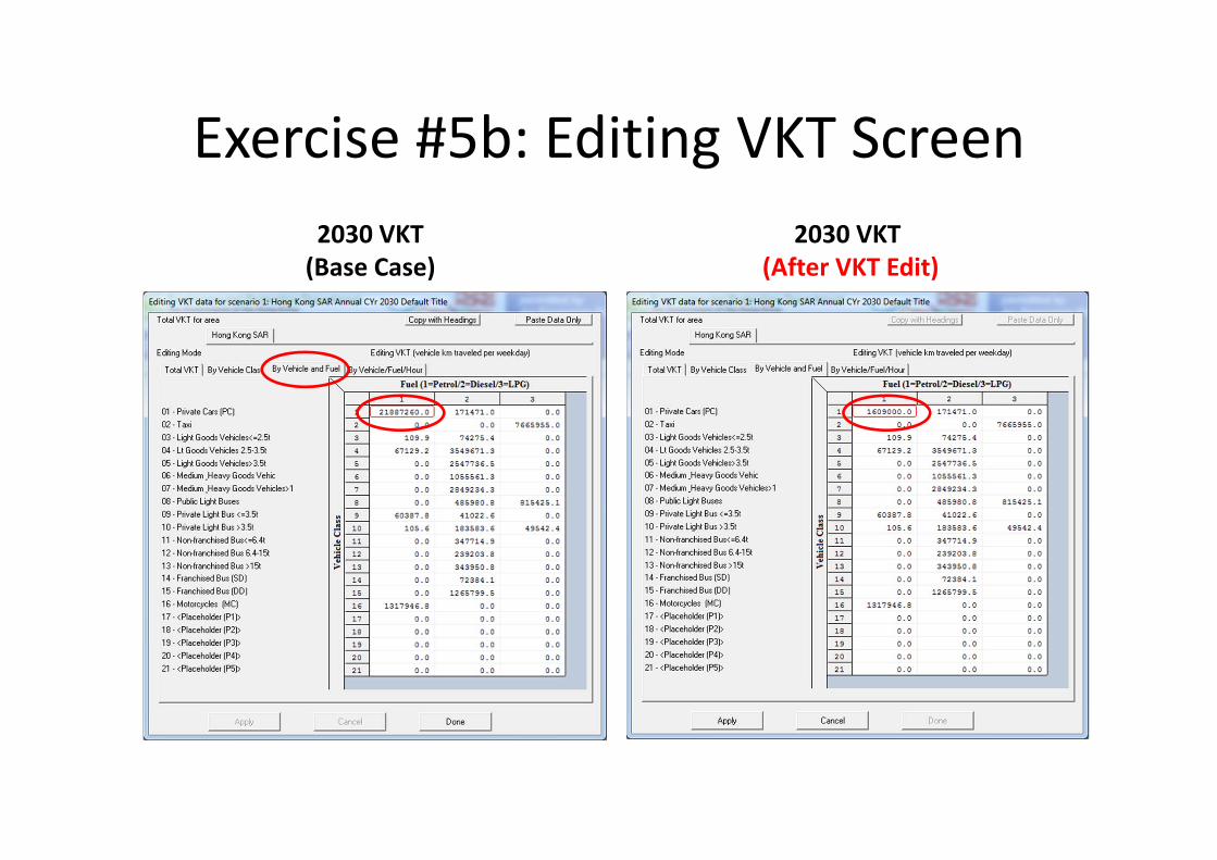
Exercise #5b: Editing VKT Screen2030 VKT (Base Case)
2030 VKT(After VKT Edit)
Exercise #5c: Changing VKT ‐Comparison of #5a and #5b Output
• Problem: determine difference in NOx running and starting exhaust emissions output from Exercises #5a and #5b for petrol private cars.
• Purpose: examine results from alternate VKT edit approaches
• Extract/compare NOx running and starting exhaust emissions from Text/*.CSV. Use values for the day. – Note: day is at bottom of CSV after results by hour– Note: you’ll need to add results for NCAT and CAT

Exercise #5c: SolutionProcess Base #5a: Pop‐adjusted
VKT#5b: VKT direct
Vehicles 783,924 57,629 783,924
VKT 21,887,260 1,609,000 1,609,000
Trips 1,176,004 86,452 1,176,004
NOx Run Exhaust (tonne/day)
0.2273 0.0167 0.0167
Nox Start Exhaust(tonne/day)
0.0441 0.0032 0.0441
Notes:Results show how the model adjusted trips in Exercise #5a, thus, starting exhaust as well. Running exhaust emissions do not differ. Exercise #5b shows it is possible to directly input VKT into EMFAC‐HK; however, it is generally not recommended to do this independent of vehicle population because of the desire to properly estimate start and evaporative emissions tied to the size of the vehicle fleet.
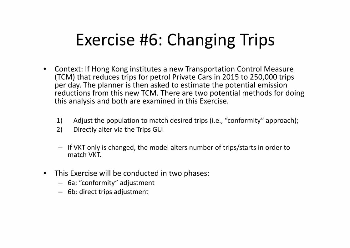
Exercise #6: Changing Trips• Context: If Hong Kong institutes a new Transportation Control Measure
(TCM) that reduces trips for petrol Private Cars in 2015 to 250,000 trips per day. The planner is then asked to estimate the potential emission reductions from this new TCM. There are two potential methods for doing this analysis and both are examined in this Exercise.
1) Adjust the population to match desired trips (i.e., “conformity” approach); 2) Directly alter via the Trips GUI
– If VKT only is changed, the model alters number of trips/starts in order to match VKT.
• This Exercise will be conducted in two phases: – 6a: “conformity” adjustment– 6b: direct trips adjustment
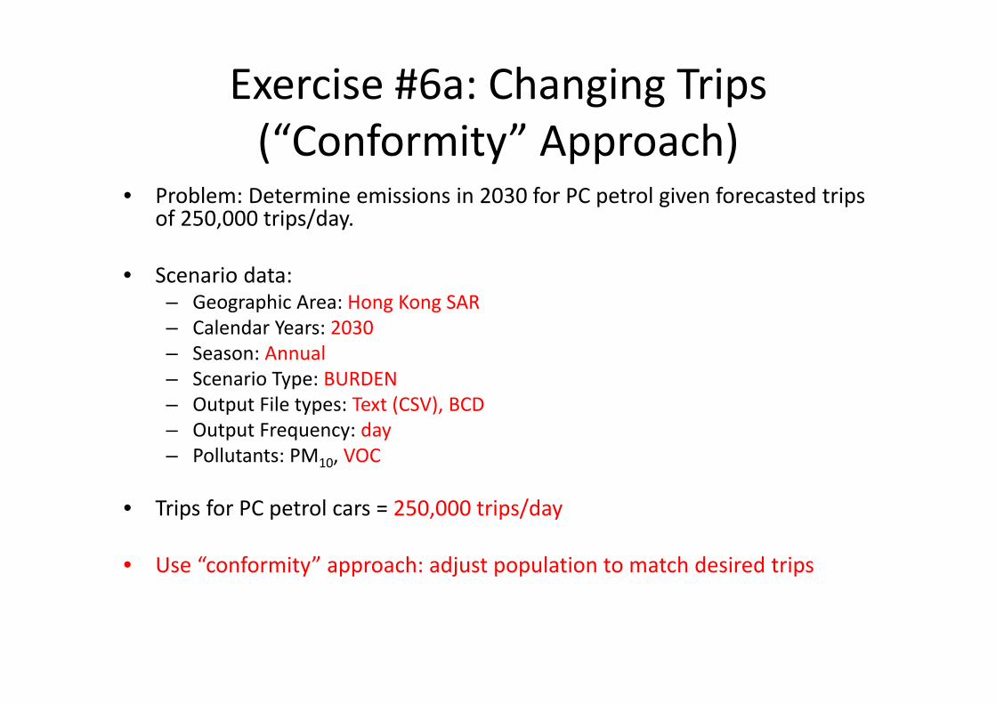
Exercise #6a: Changing Trips (“Conformity” Approach)
• Problem: Determine emissions in 2030 for PC petrol given forecasted trips of 250,000 trips/day.
• Scenario data: – Geographic Area: Hong Kong SAR– Calendar Years: 2030– Season: Annual– Scenario Type: BURDEN– Output File types: Text (CSV), BCD– Output Frequency: day– Pollutants: PM10, VOC
• Trips for PC petrol cars = 250,000 trips/day
• Use “conformity” approach: adjust population to match desired trips
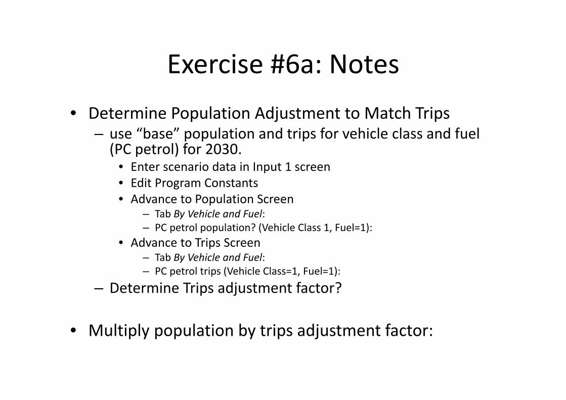
Exercise #6a: Notes• Determine Population Adjustment to Match Trips
– use “base” population and trips for vehicle class and fuel (PC petrol) for 2030.
• Enter scenario data in Input 1 screen • Edit Program Constants • Advance to Population Screen
– Tab By Vehicle and Fuel: – PC petrol population? (Vehicle Class 1, Fuel=1):
• Advance to Trips Screen – Tab By Vehicle and Fuel:– PC petrol trips (Vehicle Class=1, Fuel=1):
– Determine Trips adjustment factor?
• Multiply population by trips adjustment factor:

Exercise #6a: Base Case Values2030 Population by Fuel
783,924 vehicles (gas/petrol)2030 Trips by Fuel
1,176,004 trips (gas/petrol)

Exercise #6a: Trips Adjustment using Population
• Find “base” population and trips for vehicle class and fuel (PC petrol) for 2030: – Population (2030): 783,924 vehicles– Trips (2030 base): 1,176,004 trips
• Determine Trips adjustment factor:– 250,000/ 1,176,004 = 0.2126
• Multiply population by factor:– 783,924 x 0.2126 = 166,650 vehicles

Exercise #6a: Population Edits2030 Population
(Base Case)2030 Population
(Edited for Trips Match)

Exercise #6a: Verify Trips Adjustment2030 Trips (Base Case)
2030 Trips(After Pop Edit)

Exercise #6a: VKT Adjustment after Population Adjustment
2030 VKT (Base Case)
2030 VKT(After Pop Edit)

Exercise #6b: Changing Trips (Directly)
• Problem: Determine emissions in 2030 for PC petrol (Vehicle Class 1) given a forecast of 250,000 trips/day.
• Scenario data: – Geographic Area: Hong Kong SAR– Calendar Years: 2030– Season: Annual– Scenario Type: BURDEN– Output File types: Text (CSV), BCD– Output Frequency: hourly– Pollutants: PM10, VOC
• Trips for PC petrol cars = 250,000
• Direct entry of new trips
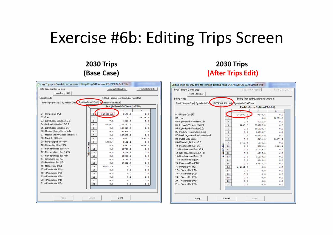
Exercise #6b: Editing Trips Screen2030 Trips(Base Case)
2030 Trips(After Trips Edit)

Exercise #6c: Changing VKT ‐Comparison of #6a and #6b Output
• Problem: determine difference in NOx running and starting exhaust emissions output from Exercises #6a and #6b for PC petrol cars.
• Purpose: examine results from alternate trip edit approaches
• Extract/compare NOx running and starting exhaust emissions from Test/*.CSV. Use values for the day.– Note: you’ll need to add results for NCAT and CAT
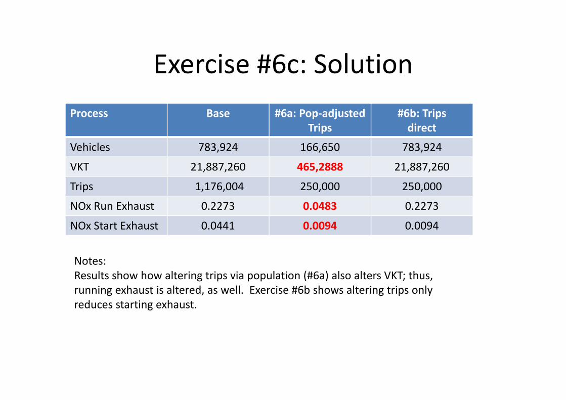
Exercise #6c: SolutionProcess Base #6a: Pop‐adjusted
Trips#6b: Trips direct
Vehicles 783,924 166,650 783,924
VKT 21,887,260 465,2888 21,887,260
Trips 1,176,004 250,000 250,000
NOx Run Exhaust 0.2273 0.0483 0.2273
NOx Start Exhaust 0.0441 0.0094 0.0094
Notes:Results show how altering trips via population (#6a) also alters VKT; thus, running exhaust is altered, as well. Exercise #6b shows altering trips only reduces starting exhaust.

Exercise #7: Speed Distributions
• Hong Kong has developed a TCM, which requires medium and heavy goods vehicles to only travel between midnight (0‐hr) and 8 a.m. and from 10 p.m. to midnight. 5% of the VKT occurs at average speed 1‐8 km/hr (Speed Bin #1 in GUI); 25% at 24‐32 km/hr (Speed Bin #4); 20% at 48‐56 km/hr (Speed Bin #7), 25% at 56‐64 km/hr (Speed Bin #8), and 25% at 64‐72 km/hr (Speed Bin #9).
• What is the effect on NOx running exhaust emissions from this change?
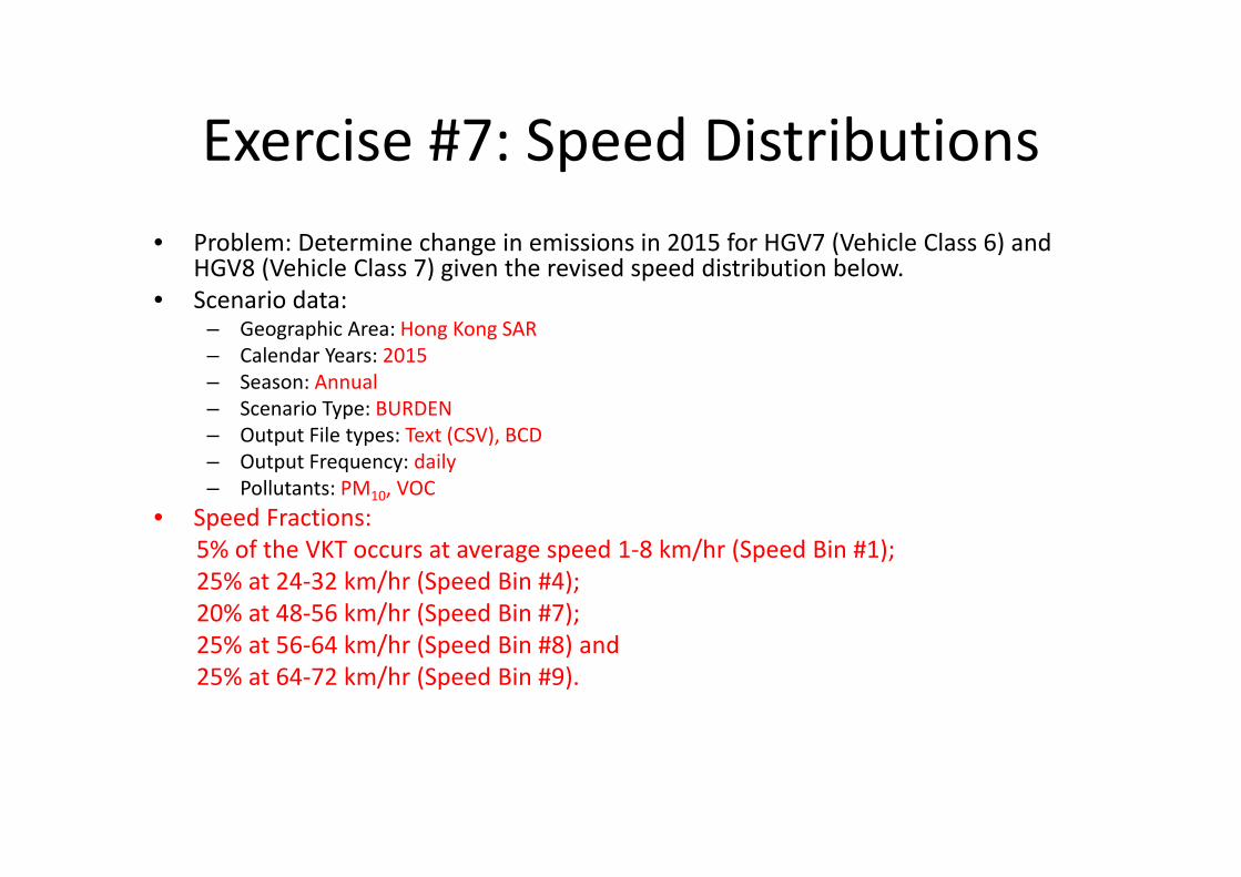
Exercise #7: Speed Distributions• Problem: Determine change in emissions in 2015 for HGV7 (Vehicle Class 6) and
HGV8 (Vehicle Class 7) given the revised speed distribution below. • Scenario data:
– Geographic Area: Hong Kong SAR– Calendar Years: 2015– Season: Annual– Scenario Type: BURDEN– Output File types: Text (CSV), BCD– Output Frequency: daily– Pollutants: PM10, VOC
• Speed Fractions: 5% of the VKT occurs at average speed 1‐8 km/hr (Speed Bin #1); 25% at 24‐32 km/hr (Speed Bin #4); 20% at 48‐56 km/hr (Speed Bin #7); 25% at 56‐64 km/hr (Speed Bin #8) and 25% at 64‐72 km/hr (Speed Bin #9).

Exercise #7: Profiles/Speed Tab
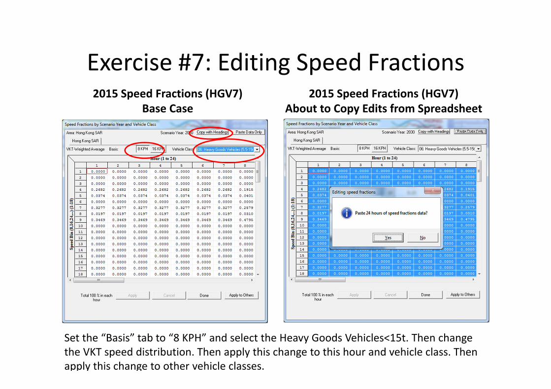
Exercise #7: Editing Speed Fractions2015 Speed Fractions (HGV7)
Base Case2015 Speed Fractions (HGV7)
About to Copy Edits from Spreadsheet
Set the “Basis” tab to “8 KPH” and select the Heavy Goods Vehicles<15t. Then change the VKT speed distribution. Then apply this change to this hour and vehicle class. Then apply this change to other vehicle classes.
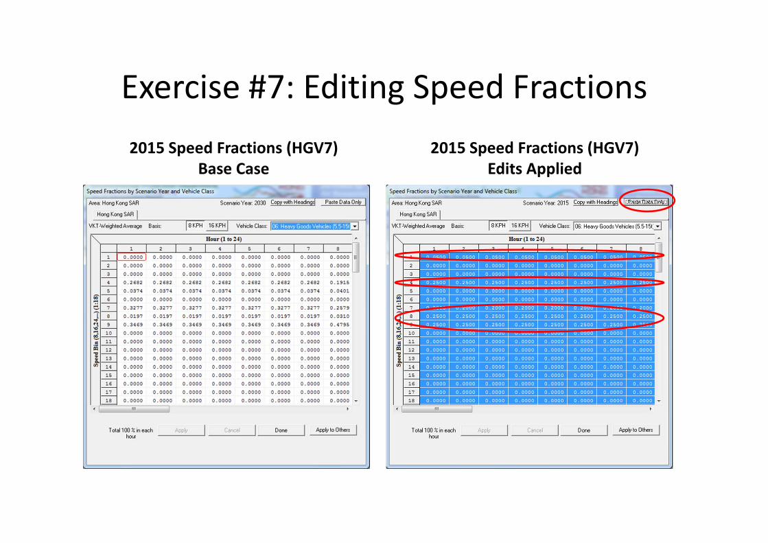
Exercise #7: Editing Speed Fractions2015 Speed Fractions (HGV7)
Base Case2015 Speed Fractions (HGV7)
Edits Applied

Exercise #7: Apply Speed Fraction Edits to Other Hours
Apply Edit to Another Veh Class Apply Edit to HGV8

Exercise #7: Solution
Exercise #8: Changing RH
• Context: This exercise shows how the user can change the relative humidity for an area of concern, say, area near a weather station, P, in 2015. It also provides the users
• Problem: Set up a base run for 2015 calendar year for Hong Kong. Include a second scenario, replacing the annual relative humidity values with the annual values provided on RH.XLS.

Exercise #8: Entering Different Relative Humidity Values
• Scenario data: – Scenario #1
• Geographic Area: Hong Kong SAR• Calendar Years: 2015• Season: Annual• Scenario Type: BURDEN• Output File types: Text (CSV), BCD• Output Frequency: daily• Pollutants: PM10, VOC
– Scenario #2: Replace annual Relative Humidity Values with values from RH.XLS
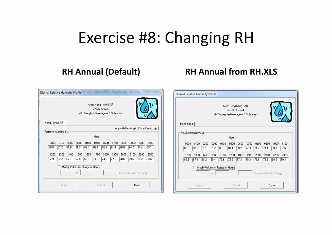
Exercise #8: Changing RH
RH Annual (Default) RH Annual from RH.XLS
This example shows how to choose and edit an alternate base year and data; then, perform a forecast of these data. The example selects an alternate baseline year (Calendar Year 2014); performs a 5% adjustment to the petrol base population; then forecasts the inventory for Calendar Year 2030.
Suggested steps:
1) Run EMFAC-HK V3.1
2) Select “File” and click “New” from the Menu
3) On Tab "MAIN", click “Add New Scenario”.
Exercise #9: Alternate Base Year

Exercise #9: Alternate Base Year

4) On Tab "INPUT1", under Step 2a - Target Years, click “Select”
5) On the "Target Year Selection" screen, click "2030" in the Available column; then, click ">". The target year 2030 should appear in the "Included" column. Click “OK”.
Exercise #9: Alternate Base Year

Exercise #9: Alternate Base Year

6) On Tab “INPUT 1”, under Step 2b – Alternate Baseline Yr” is no longer “grayed out”. Click “Select” and proceed to selecting an alternate baseline year.
7) On the “Alternate Baseline Yr Selection" screen, click "2014" in the Available column; then, click ">". The alternate baseline year of “2014” should appear in the "Included" column. Click “OK”.
Exercise #9: Alternate Base Year

Exercise #9: Alternate Base Year

8) The updated Step 2a – Target Years and Step 2b – Alternate Baseline Yrboxes should now both be updated, as indicated below. At Step 3, keep the Season or Month selection as “Annual”. Click “Next” to proceed to the screen titled Input 2.
Exercise #9: Alternate Base Year

9) In Input 2 screen, click “Default Title” to change the Step 4 -Scenario Title for Reports to reflect the concerned scenario.
Exercise #9: Alternate Base Year
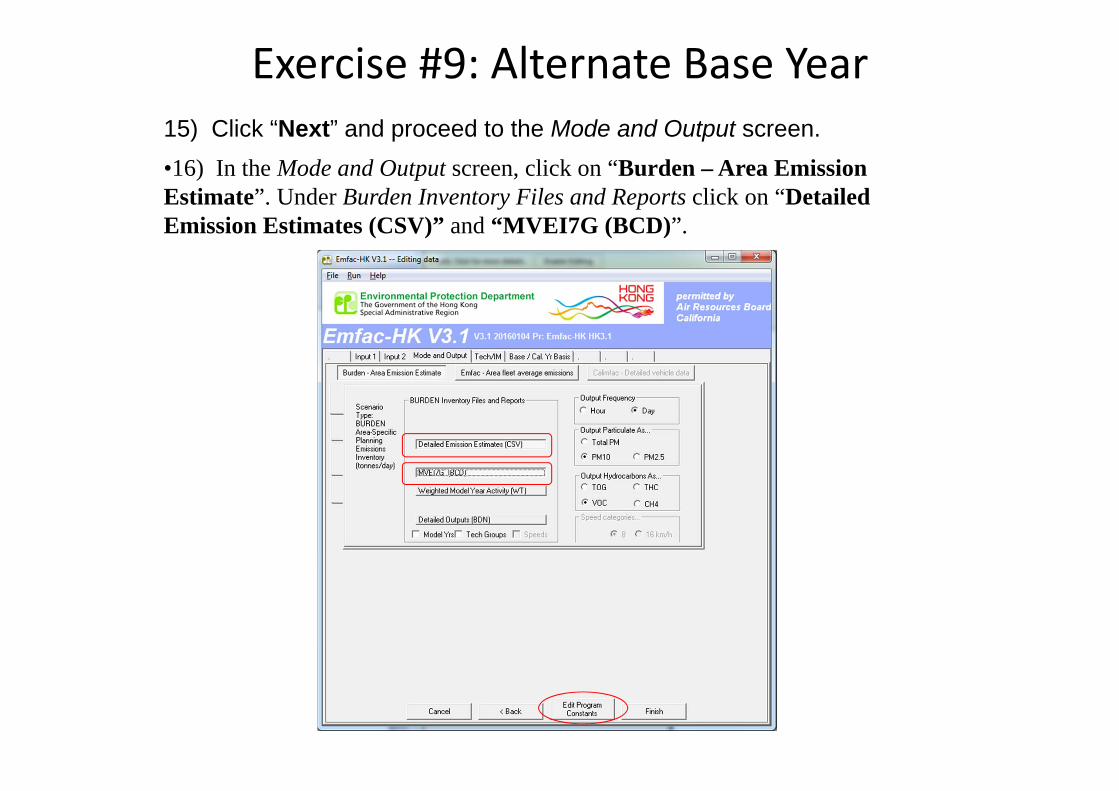
15) Click “Next” and proceed to the Mode and Output screen.•16) In the Mode and Output screen, click on “Burden – Area Emission Estimate”. Under Burden Inventory Files and Reports click on “Detailed Emission Estimates (CSV)” and “MVEI7G (BCD)”.
Exercise #9: Alternate Base Year

17) Click “Edit Program Constants” to advance to the next screen, which is the Tech/IM screen.
18) Click “Next” at the Tech/IM Screen to advance to the Base/Targ Yrscreen.
19) We will now perform edits to the Alternate Baseline Data: on the Base/Targ Yr Screen click on “2014 (Alt Baseline Pop)” to select the alternate baseline data for editing. Once the selection is made, notice that the tab has been relabeled to Base Yr Basis (2014), and the Population tab appears on the Tab Strip.
Exercise #9: Alternate Base Year

Exercise #9: Alternate Base Year
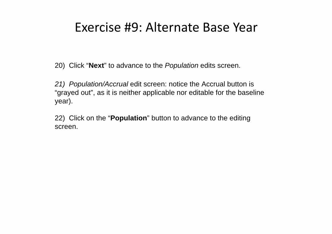
20) Click “Next” to advance to the Population edits screen.
21) Population/Accrual edit screen: notice the Accrual button is “grayed out”, as it is neither applicable nor editable for the baseline year).
22) Click on the “Population” button to advance to the editing screen.
Exercise #9: Alternate Base Year

Notice the “Accrual” button is grayed out.
Exercise #9: Alternate Base Year
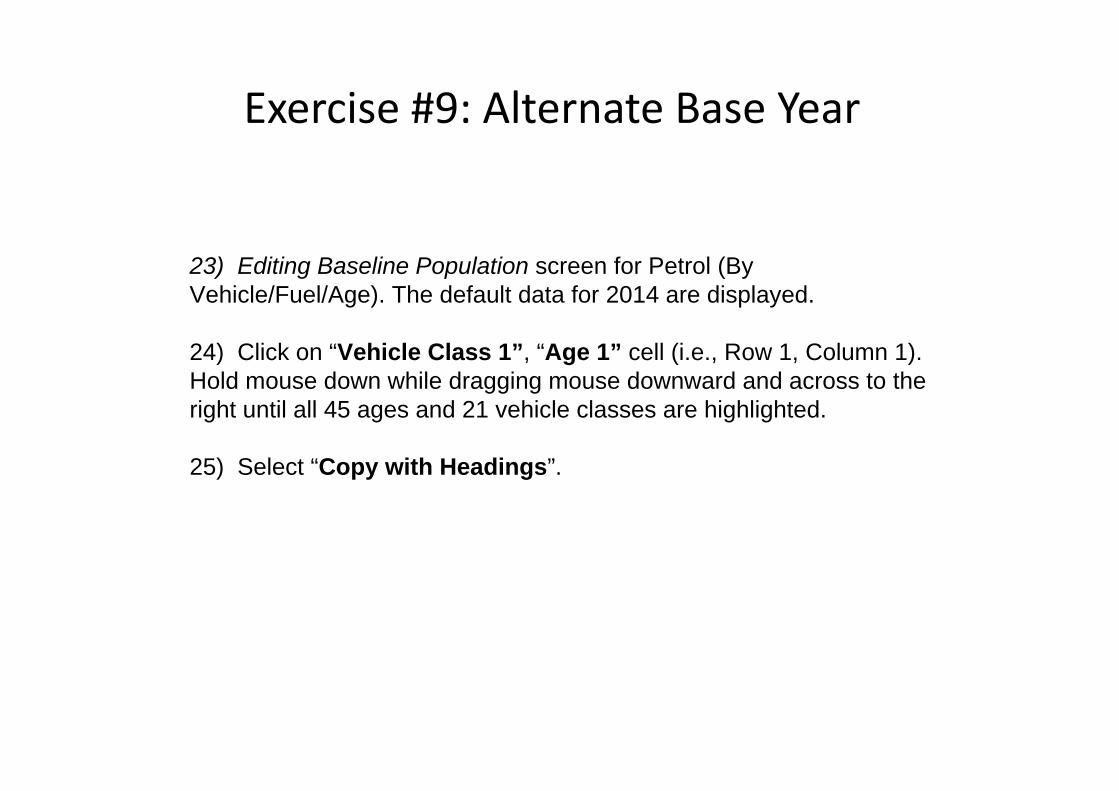
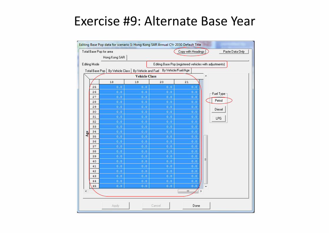
23) Editing Baseline Population screen for Petrol (By Vehicle/Fuel/Age). The default data for 2014 are displayed.
24) Click on “Vehicle Class 1”, “Age 1” cell (i.e., Row 1, Column 1). Hold mouse down while dragging mouse downward and across to the right until all 45 ages and 21 vehicle classes are highlighted.
25) Select “Copy with Headings”.
Exercise #9: Alternate Base Year
Exercise #9: Alternate Base Year

26) Open a Microsoft Excel blank spreadsheet. Paste data into Cell A1. Paste data again at Cell C24 (a formula will be used to edit this portion of the data)
27) Adjust column width of “A”, so vehicle class label can be seen.
28) At Cell B25, enter the formula “=B2*1.05”. Copy this formula to the data range (C25:AT45). Values highlighted below in yellow with “blue” text illustrate the formula cells.
Exercise #9: Alternate Base Year

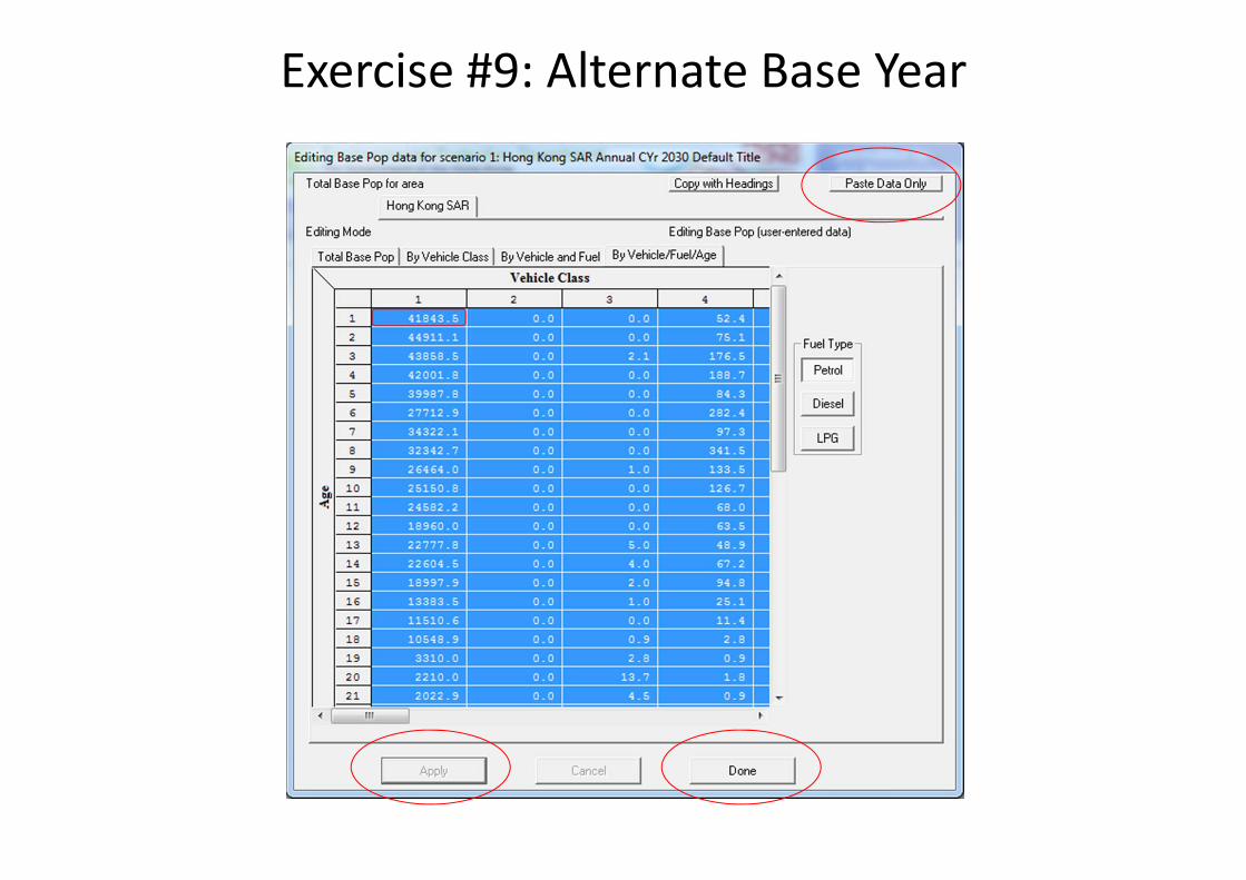
29) Highlight C25:AT25 with the mouse (i.e, the “yellow” portion above entending to Age 45), then type “Ctrl-C” to copy to the buffer.
30) Return to EMFAC-HK and click “Paste Data Only”. Then “Apply”. Then “Done”
Exercise #9: Alternate Base Year
Exercise #9: Alternate Base Year
17) Click “Finish”
18) At the MAIN screen, click “Save As” to save and name the input file to an appropriate folder. In this example, the input file was named as “Ex09.inp”.
Exercise #9: Alternate Base Year
Exercise #10: Future Projections (Accelerated Retirement)
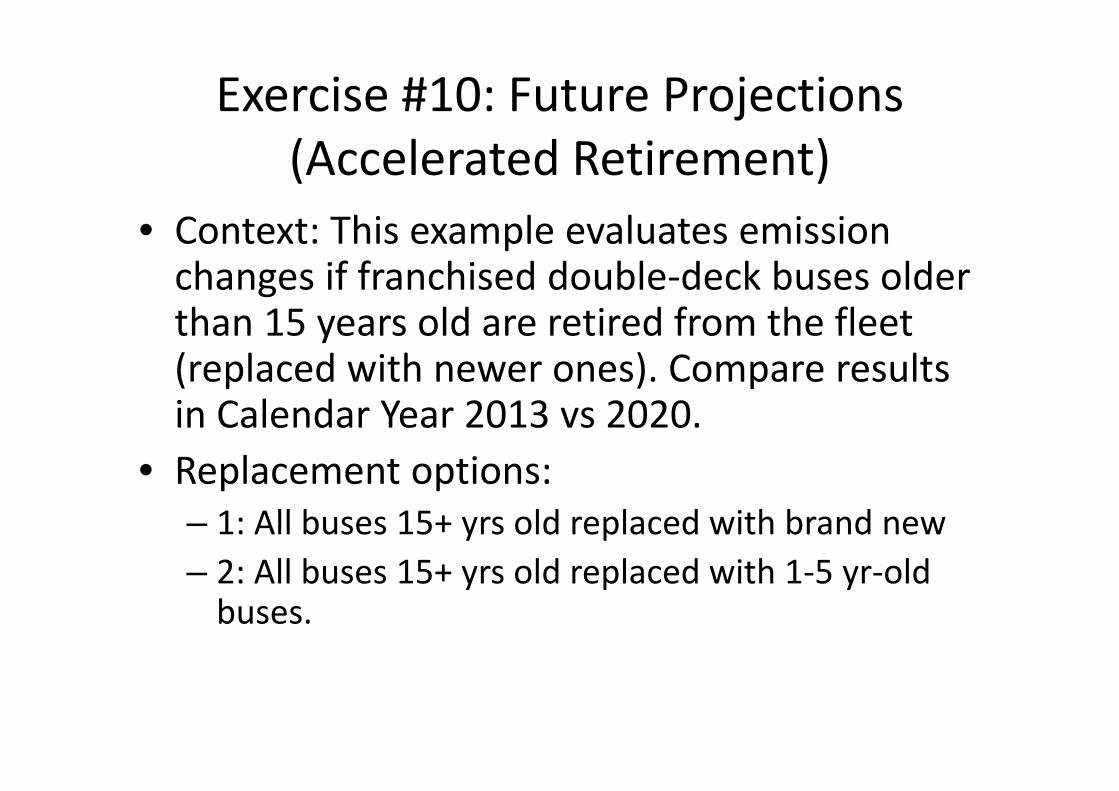
• Context: This example evaluates emission changes if franchised double‐deck buses older than 15 years old are retired from the fleet (replaced with newer ones). Compare results in Calendar Year 2013 vs 2020.
• Replacement options:– 1: All buses 15+ yrs old replaced with brand new– 2: All buses 15+ yrs old replaced with 1‐5 yr‐old buses.

Exercise #10: Future Projections
• Scenario data: – Geographic Area: Hong Kong SAR– Calendar Years: 2013, 2020– Season: Annual– Scenario Type: BURDEN– Output File types: CSV, BCD– Pollutants: PM10, VOC– Hint: Copy FBDD populations by age from GUI and implement desired program.

Exercise #11 – HK Expressway
W Kowloon Hwy Link 1167, 1169
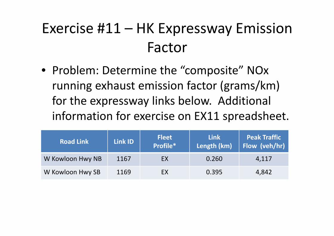
Exercise #11 – HK Expressway Emission Factor
• Problem: Determine the “composite” NOxrunning exhaust emission factor (grams/km) for the expressway links below. Additional information for exercise on EX11 spreadsheet.
Road Link Link ID FleetProfile*
LinkLength (km)
Peak TrafficFlow (veh/hr)
W Kowloon Hwy NB 1167 EX 0.260 4,117
W Kowloon Hwy SB 1169 EX 0.395 4,842
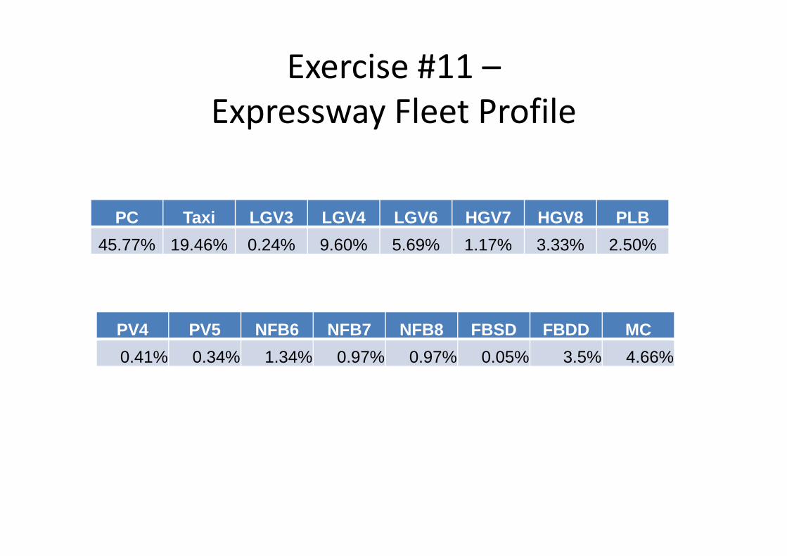
Exercise #11 –Expressway Fleet Profile
PC Taxi LGV3 LGV4 LGV6 HGV7 HGV8 PLB45.77% 19.46% 0.24% 9.60% 5.69% 1.17% 3.33% 2.50%
PV4 PV5 NFB6 NFB7 NFB8 FBSD FBDD MC0.41% 0.34% 1.34% 0.97% 0.97% 0.05% 3.5% 4.66%

Exercise #11 – Expressway Link (cont.)
• Scenario data: – Geographic Area: Hong Kong SAR– Calendar Years: 2015– Season: Annual– Scenario Type: EMFAC– Output File types: RTL– Pollutants: PM10, VOC– Temperature: 1 = 20 deg C– Relative Humidity: 1 = 70%– Speeds: 100kph, except 70kph for GV > 5.5t, FB, NFB

Exercise #11 – Expressway Link (cont.)
• Number of Runs: only 1 EMFAC‐HK run is necessary as the fleet and speed distributions are the same for each link.

Exercise #11 (cont.)
• Steps– Setup EMFAC‐HK model run– Look up emission factors for each vehicle class– Fill out Speed Fractions Table
• NOTE: speeds differ by vehicle class
– Compute “composite” (i.e., fleet‐average) emission factor
– Develop CALINE4 input parameters
Exercise #12: Build/No‐Build
• Context: This example evaluates emission changes if a roadway construction project is not implemented (i.e, build/no‐build). Projections are made what traffic will be like on the road if the project is not done.
• Roadway (2015)– Assume expressway fleet distribution from Exercise #11
• 4% reduction in vehicle population• Reduce speeds by 10kph to simulate present congestion

Exercise #12: Build/No‐Build
• Scenario data: – Geographic Area: Hong Kong SAR– Calendar Year: 2015– Season: Annual– Scenario Type: EMFAC– Output File types: RTL– Pollutants: NOx
Exercise #13: EIA Example
• Project: Extensive new roadway to be built• Sensitivity Analysis reveals 3 scenario years to evaluate: – 2021: commission year– 2026: interim year– 2036: 15 years after (peak VKT)
• 3 Roadway Groups: – EX (100 kph), UT (80 kph), PD (50 kph)– no starting emissions assumed

Exercise #13: Road Extent Example
Source: Agreement No. CE 43/2010 (HY) Central Kowloon Route – Design and Construction Estimation of Vehicular Emission for the Study Area and Determination of Worst Assessment Year by EMFAC, Appendix 4.5

Exercise #13 – EIA Example• Scenario data:
– Geographic Area: Hong Kong SAR– Calendar Years: 2021, 2026, 2036– Season: Annual– Scenario Type: EMFAC– Output File types: RTL– Pollutants: NOx– Temperature: 1 = 20 deg C– Relative Humidity: 1 = 70%– Speed Fractions: – Roads w/ posted speeds >= 70kph
• 100% at 70kph for GV > 5.5t, FB, NFB

Exercise #13: Simplifications
• For simplicity– default technology fractions– we’ll evaluate calendar year 2021 only.– Fleet mix distributions for each roadway type provided on spreadsheet

Exercise #13: EIA Example
– Setup EMFAC‐HK model runs– Look up emission factors for each vehicle class for appropriate speed
– Compute “composite” (i.e., fleet‐average) NOxrunning exhaust emission factor for each roadway type
– Develop CALINE4 input parameters